Large $p_{t}$ enhancement from freeze out

Abstract

Freeze out of particles across three dimensional space-time hypersurface is discussed in a simple kinetic model. The final momentum distribution of emitted particles, for freeze out surfaces with space-like normal, shows a non-exponential transverse momentum spectrum. The slope parameter of the $p_{t}$ distribution increases with increasing $p_{t}$, in agreement with recently measured SPS pion and $h^{-}$ spectra.

, , , , , , , and

1 Introduction

In continuum and fluid dynamical models, particles, which leave the system and reach the detectors, can be taken into account via freeze out (FO) or final break-up schemes, where the frozen out particles are formed on a 3-dimensional hypersurface in space-time. Such FO descriptions are important ingredients of evaluations of two-particle correlation data, transverse-, longitudinal-, radial-, and cylindrical- flow analyses, transverse momentum and transverse mass spectra and many other observables. The FO on a hypersurface is a discontinuity where the pre-FO equilibrated and interacting matter abruptly changes to non-interacting particles, showing an ideal gas type of behavior.

The general theory of discontinuities in relativistic flow was not worked out for a long time, and the 1948 work of A. Taub Ta48 discussed discontinuities across propagating hypersurfaces only (which have a space-like unit normal vector, $d\hat{\sigma}^{\mu}d\hat{\sigma}_{\mu}=-1$). Events happening on a propagating, (2 dimensional) surface belong to this category. An overall sudden change in a finite volume is represented by a hypersurface with a time-like normal, $d\hat{\sigma}^{\mu}d\hat{\sigma}_{\mu}=+1$. The freeze out surface is frequently a surface with time like normal. In 1987 Taub’s approach was generalized to both types of surfaces Cs87 , making it possible to take into account conservation laws exactly across any surface of discontinuity in relativistic flow. When the EoS is different on the two sides of the freeze out front these conservation laws yield changing temperature, density, flow velocity across the front CF74 ; Bu96 ; ALC98 ; AC98 ; 9ath99 .

2 Conservation laws across idealized freeze out fronts

The freeze out surface is an idealization of a layer of finite thickness (of the order of a mean free path or collision time) where the frozen-out particles are formed and the interactions in the matter become negligible.

To use well-known Cooper-Frye formula CF74

$$E\frac{dN}{d^{3}p}=\int f_{FO}(x,p;T,n,u^{\nu})\ p^{\mu}d\sigma_{\mu}$$ (1)

we have to know the post-FO distribution of frozen out particles, $f_{FO}(x,p;T,n,u^{\nu})$, which is not known from the fluid dynamical model. To evaluate measurables we have to know the correct parameters of the matter after the FO discontinuity! The post freeze out distribution need not be a thermal distribution! In fact $f_{FO}$ should contain only particles which cross the FO-front outwards, $p^{\mu}d\hat{\sigma}_{\mu}>0$, so if $d\hat{\sigma}^{\mu}$ is space-like this seriously constrains the shape of $f_{FO}$. This problem was recognized in recent years, and the first suggestions for the solution were published recently Bu96 ; ALC98 ; AC98 ; 9ath99 .

If we know the pre freeze out baryon current and energy-momentum tensor, $N_{0}^{\mu}$ and $T_{0}^{\mu\nu}\ ,$ we can calculate locally, across a surface element of normal vector $d\hat{\sigma}^{\mu}$ the post freeze out quantities, $N^{\mu}$ and $T^{\mu\nu}$, from the relations  Ta48 ; Cs87 : $[N^{\mu}\ d\hat{\sigma}_{\mu}]=0$ and $[T^{\mu\nu}\ d\hat{\sigma}_{\mu}]=0,$ where $[A]\equiv A-A_{0}$. In numerical calculations the local freeze out surface can be determined most accurately via self-consistent iteration Bu96 ; NL97 .

3 Freeze out distribution from kinetic theory

We present a kinetic model simplified to the limit where we can obtain a post FO particle momentum distribution. Let us assume an infinitely long tube with its left half ($x<0$) filled with nuclear mater and in the right vacuum is maintained. We can remove the dividing wall at $t=0$, and then the matter will expand into the vacuum. By continuously removing particles at the right end of the tube and supplying particles on the left end, we can establish a stationary flow in the tube, where the particles will gradually freeze out in an exponential rarefraction wave propagating to the left in the matter. We can move with this front, so that we describe it from the reference frame of the front (RFF).

We can describe the freeze out kinetics on the r.h.s. of the tube assuming that we have two components of our momentum distribution, $f_{free}(x,\vec{p})$ and $f_{int}(x,\vec{p})$. However, we assume that at $x=0$, $f_{free}$ vanishes exactly and $f_{int}$ is an ideal Jüttner distribution, then $f_{int}$ gradually disappears and $f_{free}$ gradually builds up.

Rescattering within the interacting component will lead to re-thermalization and re-equilibration of this component. Thus, the evolution of the component, $f_{int}$ is determined by drain terms and the re-equilibration.

We use the relaxation time approximation to simplify the description of the dynamics. Then the two components of the momentum distribution develop according to the coupled differential equations:

$$\begin{array}[]{rll}\partial_{x}f_{int}(x,\vec{p})dx=&-\Theta(p^{\mu}d\hat{\sigma}_{\mu})\frac{\cos\theta_{\vec{p}}}{\lambda}f_{int}(x,\vec{p})dx+\\ &&\\ &+\left[f_{eq}(x,\vec{p})-f_{int}(x,\vec{p})\right]\frac{1}{\lambda^{\prime}}dx,\end{array}$$ (2)

$$\begin{array}[]{rll}\partial_{x}f_{free}(x,\vec{p})dx=&+\Theta(p^{\mu}d\hat{\sigma}_{\mu})\frac{\cos\theta_{\vec{p}}}{\lambda}f_{int}(x,\vec{p})dx.\end{array}$$ (3)

Here $\cos\theta_{\vec{p}}=p^{x}/p$ in the RFF frame. The first (loss) term in eq. (2) is an overly simplified approximation to the model presented in ref. ALC98 . It expresses the fact that particles with momenta orthogonal to the FO surface ($\cos\theta_{\vec{p}}=1$) leave the system with bigger probability than particles emitted at an angle. The interacting component of the momentum distribution, described by eq. (2), shows the tendency to approach an equilibrated distribution with a relaxation length $\lambda^{\prime}$. Of course, due to the energy, momentum and particle drain, this distribution, $f_{eq}(x,\vec{p})$ is not the same as the initial Jüttner distribution, but its parameters, $n_{eq}(x)$, $T_{eq}(x)$ and $u^{\mu}_{eq}(x)$, change as required by the conservation laws.

In this case the change of the conserved quantities caused by the particle transfer from component $int$ to component $free$ can be obtained in terms of the distribution functions as:

$$dN_{i}^{\mu}=-\frac{dx}{\lambda}\int\frac{d^{3}p}{p_{0}}p^{\mu}\Theta(p^{\mu}d\hat{\sigma}_{\mu})\cos\theta_{\vec{p}}f_{int}(x,\vec{p})$$ (4)

and

$$dT_{i}^{\mu\nu}=-\frac{dx}{\lambda}\int\frac{d^{3}p}{p_{0}}p^{\mu}p^{\nu}\Theta(p^{\mu}d\hat{\sigma}_{\mu})\cos\theta_{\vec{p}}f_{int}(x,\vec{p}).$$ (5)

Due to the collision or relaxation terms $T^{\mu\nu}$ and $N^{\mu}$ change, and this should be considered in the modified distribution function $f_{int}(x,\vec{p})$.

3.1 Immediate re-thermalization limit

Let us assume that $\lambda^{\prime}\ll\lambda$, i.e. re-thermalization is much faster than particles freezing out, or much faster than parameters, $n_{eq}(x)$, $T_{eq}(x)$ and $u^{\mu}_{eq}(x)$ change. Then $f_{int}(x,\vec{p})\approx f_{eq}(x,\vec{p})$, for $\lambda^{\prime}\ll\lambda\,.$

For $f_{eq}(x,\vec{p})$ we assume the spherical Jüttner form at any $x$ including both positive and negative momentum parts with parameters $n(x),\ T(x)$ and $u_{RFG}^{\mu}(x)$. (Here $u_{RFG}^{\mu}(x)$ is the actual flow velocity of the interacting, Jüttner component, i.e. the velocity of the Rest Frame of the Gas (RFG) Bu96 ).

In this case the change of conserved quantities due to particle drain or transfer can be evaluated for an infinitesimal $dx$. The changes of the conserved particle currents and energy-momentum tensor in the RFF, eqs. (4, 5) are given in ref. ALC98 . The new parameters of distribution $f_{int}$, after moving to the right by $dx$ can be obtained from $dN_{i}^{\mu}$ and $dT_{i}^{\mu\nu}$. The differential equation describing the change of the proper particle density is ALC98 :

$$dn_{i}(x)=u_{i,RFG}^{\mu}(x)\ dN_{i,\mu}(x)\,.$$ (6)

Although this covariant equation is valid in any frame, $dN_{i}^{\mu}$ are calculated in the RFF ALC98 .

For the re-thermalized interacting component the change of Eckart’s flow velocity is given by

$$du^{\mu}_{i,E,RFG}(x)=\Delta^{\mu\nu}_{i}(x)\ \frac{dN_{i,\nu}(x)}{n_{i}(x)}\,,$$ (7)

where $\Delta^{\mu\nu}_{i}(x)=g^{\mu\nu}-u_{i,RFG}^{\mu}(x)\,u_{i,RFG}^{\nu}(x)\,$  is a projector to the plane orthogonal to $u^{\mu}_{i,RFG}(x)$, while the change of Landau’s flow velocity is ALC98

$$du^{\mu}_{i,L,RFG}(x)=\frac{\Delta^{\mu\nu}_{i}(x)\ \ dT_{i,\nu\sigma}\ \ u^{\sigma}_{i,RFG}(x)}{e_{i}+P_{i}}.$$ (8)

Although, for the spherical Jüttner distribution the Landau and Eckart flow velocities are the same, the change of this flow velocity calculated from the loss of baryon current and from the loss of energy current are different $du^{\mu}_{i,E,RFG}(x)\neq du^{\mu}_{i,L,RFG}(x)\,.$ This is a clear consequence of the asymmetry caused by the freeze out process as it was discussed in ref. ALC98 , i.e., the cut by $\Theta(p^{\mu}d\hat{\sigma}_{\mu})$ changes the particle flow and energy-momentum flow differently. This problem does not occur for the freeze out of baryonfree plasma, and we have only $du^{\mu}_{i,L}$.

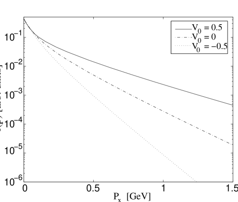
Figure 1: The local transverse momentum (here $p_{x}$) distribution for baryon free, massless gas at $p_{y}=0$, $x=100\lambda$ and $T_{0}=130\,$MeV. The transverse momentum spectrum is obviously curved due to the freeze out process, particularly for large initial flow velocities. The apparent slope parameter increases with increasing transverse momentum. This behavior agrees with observed pion transverse mass spectra at SPS na44 ; na49 .

The last task is to determine the change of the temperature parameter of $f_{int}$. From the relation $e\equiv u_{\mu}T^{\mu\nu}u_{\nu}$ we readily obtain the expression for the change of energy density

$$de_{i}(x)=u_{\mu,i,RFG}(x)\ dT^{\mu\nu}_{i}(x)\ u_{\nu,i,RFG}(x)\,,$$ (9)

and from the relation between the energy density and the temperature (see Chapter 3 in ref. Cs94 ), we can obtain the new temperature at $x+dx$. Fixing these parameters we fully determined the spherical Jüttner approximation for $f_{int}$.

The application of this model to the baryonfree and massless gas gives the following coupled set of equations:

$$\frac{d\ln{T}}{dx} = -\frac{u_{\mu}\tau^{\mu\nu}u_{\nu}}{4\sigma_{SB}}\,,$$

$$\frac{du^{\mu}}{dx} = -\frac{3}{4\sigma_{SB}}\left[\tau^{\mu\nu}-u^{\mu}u_{\sigma}\tau^{\sigma\nu}\right]u_{\nu}\,.$$

Here we use the EoS, $e=\sigma_{SB}T^{4}$,  the definition $dT^{\mu\nu}$ $=$ $-dx\,\tau^{\mu\nu}T^{4}$,   and $x$ is measured in units of $\lambda$.

Now we can find the distribution function for the noninteracting, frozen out part of particles according to equation (3). The results are shown in Fig. 1. We would like to note that now $f_{int}(x,\vec{p})$ does not tend to the cut Jüttner distribution in the limit $x\rightarrow\infty$. Furthermore, we obtain that $T\rightarrow 0$, when $x\rightarrow\infty$ ALC98 . So, $f_{int}(x,\vec{p})=\frac{1}{(2\pi\hbar)^{3}}\exp[(\mu-p^{\nu}u_{\nu})/T]\rightarrow 0$, when $x\rightarrow\infty$. Thus, all particles freeze out in the present model, but such a physical FO requires infinite distance (or time). This second problem may also be removed by using volume emission model discussed in 9ath99 .

4 Conclusions

In a simple kinetic model we evaluated the freeze out distribution, $f_{free}(x,p)$, for stationary freeze out across a surface with space-like normal vector, $d\hat{\sigma}^{\mu}d\hat{\sigma}_{\mu}<0$. In this model particles penetrating the surface outwards were allowed to freeze out with a probability $\sim\cos\theta_{\vec{p}}$, and the remaining interacting component is assumed to be instantly re-thermalized. The three parameters of the interacting component, $f_{int}$, are obtained in each time step. The density of the interacting component gradually decreases and disappears, the flow velocity also decreases and the energy density decreases. The temperature, as a consequence of the gradual change in the emission mechanism, gradually decreases.

The arising post freeze out distribution, $f_{free}$ is a superposition of cut Jüttner type of components, from a series of gradually slowing down Jüttner distributions. This leads to a final momentum distribution, with a more dominant peak at zero momentum and a forward halo, Fig. 1. In this rough model a large fraction ($\sim 95\%$) of the matter is frozen out by $x=3\lambda$, thus, the distribution $f_{free}$ at this distance can be considered as a first estimation of the post freeze out distribution. One should also keep in mind that the model presented here does not have realistic behavior in the limit $x\longrightarrow\infty$, due to its one dimensional character.

These studies indicate that more attention should be paid to the final freeze out process, because a realistic freeze out description may lead to large $p_{t}$ enhancement na44 ; na49 as the considerations above indicate (Fig. 1). For accurate estimates more realistic models should be used. In case of rapid hadronization of QGP and simultaneous freeze out, the idealization of a freeze out hypersurface may be justified, however, an accurate determination of the post freeze out hadron momentum distribution would require a nontrivial dynamical calculation.

References

- (1) A.H. Taub, Phys. Rev. 74 (1948) 328.
- (2) L.P. Csernai, Sov. JETP 65 (1987) 216; Zh. Eksp. Theor. Fiz. 92 (1987) 379.
- (3) F. Cooper and G. Frye, Phys. Rev. D 10 (1974) 186.
- (4) K.A. Bugaev, Nucl. Phys. A606 (1996) 559.
- (5) Cs. Anderlik, Zs. Lázár, V.K. Magas, L.P. Csernai, H. Stöcker and W. Greiner, (nucl-th/9808024) Phys. Rev. C 59 (99) 388.
- (6) Cs. Anderlik, L.P. Csernai, F. Grassi, W. Greiner, Y. Hama, T. Kodama, Zs. Lázár, V.K. Magas and H. Stöcker, (nucl-th/9806004) Phys. Rev. C 59 (1999) in press May 1 issue.
- (7) Cs. Anderlik, L.P. Csernai, F. Grassi, W. Greiner, Y. Hama, T. Kodama, Zs. Lázár, V.K. Magas and H. Stöcker in preparation.
- (8) L.P. Csernai: Introduction to Relativistic Heavy Ion Collisions (Wiley, 1994).
- (9) J.J. Neumann, B. Lavrenchuk and G. Fai, Heavy Ion Phys. 5 (1997) 27.
- (10) Nu Xu, et al., (NA44), Nucl. Phys. A610 (1997) 175c. (pion spectra in Figs. 4 and 6.)
- (11) P.G. Jones, et al., (NA49), Nucl. Phys. A610 (1997) 188c. ( spectra in Fig. 2.)