The $\pi NN$ vertex function in a meson-theoretical model

Abstract

The $\pi NN$ vertex function is calculated within a dispersion theoretical approach, including both $\pi\rho$ and $\pi\sigma$ intermediate states, where the $\sigma$ meson is an abbreviation for a correlated pion pair in a relative S-wave with isospin I=0. A strong coupling between the $\pi\sigma$ and $\pi\rho$ states is found. This leads to a softening of the $\pi NN$ form factor. In a monopole parameterization, a cut-off $\Lambda\approx 800\,$MeV is obtained as compared to $\Lambda\approx 1000\,$MeV using $\pi\rho$ intermediate states only.

I Introduction

NT@UW-99-27, DOE/ER/40561-67, FZJ-IKP(TH)-1999-17

The pion nucleon-nucleon vertex function is needed in many different places in hadron physics, such as the nucleon-nucleon interaction [1], pion-nucleon scattering and pion photoproduction [2, 3], deep-inelastic scattering [4], and as a possible explanation of the Goldberger-Treiman discrepancy [5, 6, 7, 8, 9]. Commonly, one represents the vertex function by a phenomenological form factor. The cut-off parameters employed in the various calculations range from $\Lambda^{(1)}_{\pi NN}=300$ MeV in pion photoproduction to $\Lambda^{(1)}_{\pi NN}=1700$ MeV in some One-Boson Exchange models of the nucleon-nucleon interaction, assuming a monopole representation (i.e. $n=1$ in Eq. (15), see below). The Skyrmion model [10, 11] gives $\Lambda^{(1)}_{\pi NN}=860$ MeV. A lattice gauge calculation gets $\Lambda^{(1)}_{\pi NN}=750\pm 140$ MeV [12].

Unfortunately, the $\pi NN$ form factor cannot be determined experimentally. It is an off-shell quantity which is inherently model-dependent. For a given model, the form factor – besides being a parametrization of the vertex function – summarizes those processes which are not calculated explicitly.

The simplest class of meson-theoretical models of the nucleon-nucleon interaction includes the exchange of one meson only. In these models, one needs ”hard” form factors for the following reason. In One-Boson Exchange potentials, the tensor force is generated by one-pion and one-rho exchange. A cut-off below 1.3 GeV would reduce the tensor force too strongly and make a description of the quadrupole moment of the deuteron impossible [13, 1].

This situation changes when the exchange of two correlated bosons between nucleons is handled explicitly. The exchange of an interacting $\pi\rho$ pair generates additional tensor strength at large momentum transfers. This implies softer cut-offs for the genuine one-pion exchange [14, 15].

Meson theory allows to undress the phenomenological form factors at least partly by calculating those processes which contribute most strongly to the long range part of the vertex functions [14, 16]. A physically very transparent way to include the most important processes is given by dispersion theory. The imaginary part of the form factor in the time-like region is given by the unitarity cuts. In principle, one should consider the full three-pion continuum. A reasonable approximation is to reduce the three-body problem to an effective two-body problem by representing the two-pion subsystems by effective mesons [17]. An explicit calculation of the selfenergy of the effective meson incorporates the effects of three-body unitarity. In the case of the pion-nucleon form factor, one expects that $\pi\rho$ and $\pi\sigma$ intermediate states are particularly relevant. Here, ”$\sigma$ ” is understood as an abbreviation for the isoscalar two-pion subsystem. In many early calculations [7, 18], the effect of the $\pi\sigma$ intermediate states was found to be negligible. In these calculations, a scalar $\sigma\pi\pi$ coupling has been used. Nowadays, such a coupling is disfavored because it is not chirally invariant. In the meson-theoretical model for pion-nucleon scattering of Ref. [19], the exchange of two correlated mesons in the t-channel has been linked to the two-pion scattering model of Ref. [20]. The resulting effective potential can be simulated by the exchange of an effective sigma-meson in the t-channel, if a derivative sigma two-pion coupling is adopted.

In the present work, we want to investigate the effect of the pion-sigma channel on the pion form factor using a derivative coupling.

The meson-meson scattering matrix $T$ is an essential building block of our model. Formally, the scattering matrix is obtained by solving the Bethe-Salpeter equation, $T=V+VGT,$ starting from a pseudopotential $V$. Given the well-known difficulties in solving the four-dimensional Bethe Salpeter equation, one rather solves three-dimensional equations, such as the Blankenbecler-Sugar equation (BbS) [21] or related ones [22, 23]. The two-body propagator $G$ is chosen to reproduce the two-particle unitarity cuts in the physical region. The imaginary part of $G$ is uniquely defined in this way, but for the real part, there is complete freedom which leads to an infinite number of reduced equations [23]. The energies of the interacting particles are well-defined for on-shell scattering only. For off-shell scattering, there is an ambiguity. Different choices of the energy components may affect the off-shell behaviour of the matrix elements. As long as one is exclusively interested in the scattering of one kind of particles, e.g. only pions, one can compensate the modifications of the off-shell behaviour by readjusting the coupling constants. This gets more difficult as soon as one aims for a consistent model of many different reactions. Moreover, in the calculation of the form factor, the scattering kernel $V$ may have singularities which do not agree with the physical singularities due to e.g. three-pion intermediate states [24].

In contrast to the Blankenbecler-Sugar reduction, time-ordered perturbation theory (TOPT)determines the off-shell behaviour uniquely. Moreover, only physical singularities corresponding to the decay into multi-meson intermediate states can occur [25]. For the present purpose, we therefore will employ time-ordered perturbation theory.

II The Meson–Meson Interaction Model

The Feynman diagrams defining the pseudopotentials for $\pi\rho$ and $\pi\sigma$ scattering are shown in Fig. 1 and Fig. 2. We include both pole diagrams as well as t-channel and u-channel exchanges. The transition potential is given by one-pion exchange in the t-channel (see Fig. 3). In Ref. [14], $\pi\rho$ scattering has been investigated neglecting the $A_{1}$-exchange in the u-channel.

FIG. 1.: Diagrams describing the $\pi\rho\rightarrow\pi\rho$ potential

FIG. 2.: Diagrams describing the $\pi\sigma\rightarrow\pi\sigma$ potential

FIG. 3.: Diagram describing the $\pi\rho\rightarrow\pi\sigma$ transition potential

The $\pi\pi\rho$ and $A_{1}\pi\rho$ interactions are chosen according to the Wess-Zumino Lagrangian [26] with $\kappa=\frac{1}{2}$. The two-pion sigma vertex is defined by a derivative coupling [19]. For the three-sigma vertex we take a scalar coupling [19]. The Lagrangians employed read explicitly:

$${\cal L}_{\pi\pi\rho} = -g_{\pi\pi\rho}\ (\vec{\pi}\times\partial_{\mu}\vec{\pi})\cdot\vec{\rho}^{\,\mu}$$ (1)

$${\cal L}_{\rho\rho\rho} = \frac{1}{2}g_{\pi\pi\rho}(\partial_{\mu}\vec{\rho}_{\nu}-\partial_{\nu}\vec{\rho}_{\mu})\cdot(\vec{\rho}^{\,\mu}\times\vec{\rho}^{\,\nu})$$ (2)

$${\cal L}_{A_{1}\pi\rho} = \frac{g_{\pi\pi\rho}}{m_{A_{1}}}\Big{[}(\vec{A}_{\mu}\times\partial_{\nu}\vec{\pi})-(\vec{A}_{\nu}\times\partial_{\mu}\vec{\pi})$$ (4)

$$+\frac{1}{2}\left\{\vec{\pi}\times(\partial_{\mu}\vec{A}_{\nu}-\partial_{\nu}\vec{A}_{\mu})\right\}\Big{]}(\partial^{\mu}\vec{\rho}^{\,\nu}-\partial^{\nu}\vec{\rho}^{\,\mu})$$

$${\cal L}_{\omega\pi\rho} = \frac{g_{\omega\pi\rho}}{m_{\omega}}\ \epsilon^{\mu\alpha\lambda\nu}\partial_{\alpha}\vec{\rho}_{\mu}\ \partial_{\lambda}\vec{\pi}\ \omega_{\nu}$$ (5)

$${\cal L}_{\pi\pi\sigma} = \frac{f}{2m_{\pi}}\ \partial_{\mu}\vec{\pi}\cdot\partial^{\mu}\vec{\pi}{\sigma}$$ (6)

$${\cal L}_{\sigma\sigma\sigma} = g_{\sigma\sigma\sigma}m_{\sigma}\ {\sigma}{\sigma}{\sigma}.$$ (7)

The completely antisymmetric tensor has the component $\epsilon_{0123}=+1$.

In the presence of derivative couplings, the canonical momenta conjugate to the fields $\Phi_{k}$,

$$\pi_{k}=\frac{\delta{\cal L}}{\delta\dot{\Phi}_{k}},$$

receive contributions from the interaction Lagrangian. The corresponding Hamiltonian density

$${\cal H}\ =\ \sum_{k}\pi_{k}\dot{\Phi}_{k}\ -\ {\cal L}$$ (8)

consists of the ususal terms plus additional contact terms:

$${\cal H}\ =\ {\cal H}_{0}-{\cal L}_{int}+{\cal H}_{contact}.$$ (9)

The contact terms ensure that the diagrams of time-ordered perturbation theory are on-shell equivalent to the corresponding Feynman diagrams. For our model Lagrangian, the contact terms, expanded up to the order $g^{2},f^{2}$, and $fg$, are given by:

$${\cal H}_{contact} = +\frac{g_{\pi\pi\rho}^{2}}{2}(\vec{\rho}^{\,0}\times\vec{\pi})^{2}+\frac{f^{2}}{2m_{\pi}^{2}}{\sigma}^{2}\dot{\vec{\pi}}^{2}$$ (14)

$$-\frac{fg_{\pi\pi\rho}}{m_{\pi}}{\sigma}\dot{\vec{\pi}}\cdot(\vec{\rho}^{\,0}\times\vec{\pi})$$

$$+\frac{g_{\omega\pi\rho}^{2}}{2m_{\omega}^{4}}\left\{\epsilon_{ijk}(\partial^{i}\vec{\rho}^{\,j})(\partial^{k}\vec{\pi})\right\}^{2}$$

$$+\frac{2g_{\pi\pi\rho}^{2}}{m_{A_{1}}^{4}}\left\{\partial_{\nu}\vec{\pi}\times(\dot{\vec{\rho}}^{\,\nu}-\partial^{\nu}\vec{\rho}^{\,0})\right\}^{2}$$

$$+\frac{g_{\pi\pi\rho}^{2}}{2m_{A_{1}}^{2}}\left\{(\partial_{k}\vec{\rho}^{\,0}-\dot{\vec{\rho}}_{k})\times\vec{\pi}\right\}^{2}$$

The Feynman diagrams are replaced by the corresponding time-ordered diagrams and a contact diagram, as e.g. shown in Fig. 4 for the case of pion-rho scattering via pion exchange in the s-channel.

$\parbox[c][59.75095pt]{45.52458pt}{\psfig{height=56.9055pt,width=42.67912pt}}=\parbox[c]{45.52458pt}{\psfig{height=56.9055pt,width=42.67912pt}}\;+\;\parbox[c]{45.52458pt}{\psfig{height=56.9055pt,width=42.67912pt}}\;+\;\parbox[c]{45.52458pt}{\psfig{height=56.9055pt,width=42.67912pt}}$

FIG. 4.: Decomposition of the pion-pole Feynman diagram into time-ordered diagrams and a contact term.

Form factors are required to ensure convergence. We choose standard monopole ($n=1$) or dipole ($n=2$) parameterizations,

$$\Gamma^{(n)}(q^{2})=\left(\frac{\Lambda^{2}-m^{2}}{\Lambda^{2}-q^{2}}\right)^{n}$$ (15)

The cut-off parameters $\Lambda^{(n)}$ and the coupling constants $\frac{g^{2}}{4\pi}$ are taken from other investigations. In detail, we employ the following constants. The coupling constant $\frac{g^{2}_{\pi\pi\rho}}{4\pi}=2.84$ can be determined from the decay $\rho\rightarrow\pi\pi$. We assume $g_{\pi\rho A_{1}}=g_{\pi\pi\rho}$ [26]. The corresponding cut-off parameters $\Lambda^{(1)}_{\pi\pi\rho}=1500$ MeV and $\Lambda^{(2)}_{\pi\rho A_{1}}=2600$ MeV have been taken from Ref. [24]. The decay $\omega\rightarrow\pi\rho\rightarrow\pi\gamma$ gives the coupling constant $\frac{g^{2}_{\pi\rho\omega}}{4\pi}=7.5$ and $\Lambda^{(2)}=2200$ MeV [27].

In the meson-theoretic model for pion-nucleon scattering of Refs. [19, 28], the following constants have been determined: $\frac{g^{2}_{\pi\pi\sigma}}{4\pi}=0.25$, $\Lambda^{(1)}_{\pi\pi\sigma}=1300$ MeV, $\frac{g^{2}_{\sigma\sigma\sigma}}{4\pi}=3.5$, $\Lambda^{(1)}_{\sigma\sigma\sigma}=2000$ MeV.

In Fig.5, we compare the half-off shell scattering kernels $V$ derived in TOPT and in the BbS reduction for a center-of-momentum energy $\sqrt{s}=1.2$ GeV. When the off-shell momentum P is equal to the incoming on-shell momentum, the potentials $V$ evaluated in the BbS reduction and in TOPT are identical (see the arrow). In the BbS reduction, the zeroth component of the momentum vectors is not well-defined for off-shell scattering. In Fig.5 we have chosen on-energy shell components, following Ref. [14]. For the $A_{1}$ exchange (both in the s- and in the u-channel), both formalisms give fairly similar results. For the rho-exchange in the t-channel, the $S^{11}$ partial wave shows large differences: while TOPT predicts an attractive half-off shell matrix element, the BbS-reduction gets repulsive for momenta larger than 650 MeV.

FIG. 5.: Different contributions to the half off-shell potentials for $\pi\rho$ scattering at $\sqrt{s}=1.2$ GeV for various partial waves as functions of the off-shell momentum P. The arrow indicates the on-shell momentum P corresponding to $\sqrt{s}=1.2$ GeV. The solid line represents the scattering kernel $V$ of TOPT, while the dashed line refers to the BbS reduction. The dotted line shows the TOPT result omitting the contact terms. The panels show contributions of specific diagrams of Fig.1; upper left: $A_{1}$ pole diagram, middle left: $\pi$ pole diagram, lower left: $\rho-$exchange in the t-channel, upper right: $A_{1}$ u-channel exchange, middle right: $\omega$ pole diagram, lower right: $\omega$ u-channel exchange.

The singularities in the scattering kernel $V$ due to unitarity cuts are handled by chosing an appropriate path in the complex momentum plane. The scattering equation, after partial wave decomposition, reads explicitly:

$$T(p,p^{\prime})=V(p,p^{\prime})+\\ \int dkk^{2}V(p,k)G^{TOPT}(E;k)T(k,p^{\prime})$$ (16)

with

$$k=|\vec{k}|e^{-i\Phi},$$ (17)

where $\Phi$ is a suitably chosen angle [29]. $G^{TOPT}(E;k)$ denotes the two-body propagator of time-ordered perturbation theory.

The resulting $T$-matrix is shown in Fig.6 for $\sqrt{s}=0.7$ GeV and k=153 MeV for the total angular momentum J=0. The potential $V$ for pion-rho scattering is attractive (upper panel). Iterating the $\pi\rho$ diagrams by themselves, the attraction is enhanced. The inclusion of the $\pi\sigma$ channel enhances the attraction even more. This effect is due to the off-shell transition potential (middle and lower panel) which is larger than the diagonal $\pi\rho$ potential. The magnitude of the transition potential can be traced back to the interaction Lagrangian (see Fig.5). The derivative coupling favours large momentum transfers. The enhancement of the $\pi\rho-\pi\rho$ scattering matrix $T$ due to these coupled channel effects will shift the maximum of the spectral function to lower energies and thus lead to a softer form factor.

FIG. 6.: The full off-shell $T$-matrices for the transitions $\pi\rho\rightarrow\pi\rho$ (upper panels), $\pi\rho\rightarrow\sigma\pi$ (central panels), and $\sigma\pi\rightarrow\pi\rho$ (lower panels) are shown for $E_{CM}=1200$MeV and $k^{in}_{CM}=153$ MeV(solid lines) as functions of the real part of the complex off-shell momentum P. The $T$-matrix for the transition $\pi\rho\rightarrow\pi\rho$ obtained without coupling to the $\sigma\pi$ channel is given by the dashed line. For comparison, also the corresponding scattering kernels $V$ are displayed (dotted lines). The real parts of the $T$-matrices are shown on the left hand side, the imaginary parts on the right hand side.

III The Pion–Nucleon Form Factor

The present model for the $\pi NN$ vertex function F is shown in Fig. 7.

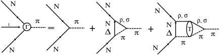
FIG. 7.: The $\pi NN$ vertex function

Before coupling to the nucleon, the pion can disintegrate into three-pion states which are summarized by both pion-sigma and pion-rho pairs. We first evaluate the vertex function in the $N\bar{N}$ channel. In this channel, the $\pi\rho$ and $\pi\sigma$ interactions can be summed. After a decomposition into partial waves, one gets:

$$F_{N\bar{N}\rightarrow\pi}=F^{\,0}_{N\bar{N}\rightarrow\pi}+\sum_{n=\rho,\,\sigma}\int dk\,k^{2}$$ (18)

$$\times f_{\pi\leftarrow\pi n}(t,k)G_{\pi n}(t,k)V_{\pi n\leftarrow N\bar{N}}(t;k,p_{0})\;.$$ (19)

Here, $\rm p_{0}$ is the subthreshold on–shell momentum of the $\rm N\bar{N}\,$–System [5]. The bare vertex is called $F^{\,0}_{N\bar{N}\rightarrow\pi}$. We have to include the self energies $\Sigma_{\rho}$ and $\Sigma_{\sigma}$ of both the $\rho$ and the $\sigma$ into the two-particle propagators $\rm G_{\pi\rho}$ and $\rm G_{\pi\sigma}$ because the vertex function is needed in the time-like region. The annihilation potential $\rm V_{\pi n\leftarrow N\bar{N}}$ has been worked out in Ref. [30]. The form factor needed for the $N\bar{N}\rightarrow\pi\rho(\sigma)$ transition has not been determined selfconsistently, but taken from Ref. [30].

The dressed meson–meson $\rightarrow$ pion vertex function $f_{\pi\leftarrow\pi n}$ is given by

$$f_{\pi\leftarrow\pi n}(t,k)=f^{\,0}_{\pi\leftarrow\pi n}(t,k)+\sum_{m=\rho,\,\sigma}\int dk^{\prime}{k^{\prime}}^{2}$$ (20)

$$\times f^{\,0}_{\pi\leftarrow\pi m}(t,k^{\prime})G_{\pi m}(t,k^{\prime})T_{\pi m\leftarrow\pi n}(t;k^{\prime},k)\;.$$ (21)

The bare vertex function is called $f^{\,0}$. The vertex function $f$ requires the off-shell elements of the $T$-matrix for meson-meson scattering $T_{\pi m\rightarrow\pi n}$ discussed in the previous chapter. Only the partial wave with total angular momentum $\rm J^{\pi}=0^{-}$ of the $N\bar{N}\rightarrow\pi$ vertex function is needed.

The form factor $\rm\Gamma(t)$ is defined as

$$\Gamma(t) = \frac{F_{N\bar{N}\rightarrow\pi}}{F^{\,0}_{N\bar{N}\rightarrow\pi}}\;.$$ (22)

Now we rely on dispersion theory to obtain the form factor $\rm\Gamma(t)$ for space-like momentum transfers t [5, 7]. We employ a subtracted dispersion relation

$$\Gamma(t) = 1+\frac{t-m_{\pi}^{2}}{\pi}\int\limits_{9m_{\pi}^{2}}^{\infty}\frac{Im\Gamma(t^{\prime})dt^{\prime}}{(t^{\prime}-t)(t^{\prime}-m_{\pi}^{2})}\;.$$ (23)

The subtraction constant ensures that the form factor is normalized to unity for $t=m_{\pi}^{2}$. The integration is cut off at $t=4\,m_{N}^{\,2}$. Larger values of $t$ would require to incorporate diagrams with cuts at larger energies. Such processes are suppressed because of the improved rate of convergence of the subtracted dispersion relation.

The imaginary part of the form factor is shown in the left part of Fig.8.

FIG. 8.: Real (right panel) and imaginary (left panel) parts of the $\pi NN$ form factor as functions of the momentum transfer t. Solid line: coupled $\pi\rho$ and $\pi\sigma$ channels; dotted line: only the $\pi\rho$ channel is considered; dashed line: rescattering in the $\pi\rho$ channel is omitted; dashed-dotted line: only the $\pi\sigma$ channel is included. The short-dashed line in the right panel refers to a monopole form factor with $\Lambda^{(1)}=800$ MeV.

We confirm earlier findings [7, 18] that the pion-sigma states by themselves, even if iterated, do not generate an appreciable contribution to the spectral function. The $\pi\rho$ intermediate states clearly dominate. Including rescattering processes in a model with only $\pi\rho$ states, one finds a large shift of the spectral function to smaller energies, which emphasizes the importance of the correlations. The new aspect of our work is the large shift induced by the coupling between $\pi\rho$ and $\pi\sigma$ states.

In Ref. [31] Holinde and Thomas introduced an effective $\pi^{\prime}$ exchange contribution to the One-Boson Exchange $NN$ interaction in a phenomenological way in order to shift part of the tensor force from the $\pi$ into the $\pi^{\prime}$ exchange. This allowed them to use a rather soft cut-off $\Lambda^{(1)}_{\pi NN}=800MeV$ to describe the $NN$ phase shifts. The maximum of the spectral function shown in Fig. 8 is located at 1.2 GeV ($t\approx 75m_{\pi}^{2}$) which coincides with the mass of the $\pi^{\prime}$. Thus the $\pi^{\prime}$ used in Ref. [31] can be interpreted in terms of a correlated coupled $\pi\rho$ and $\pi\sigma$ exchange. Note, that the form factor derived here must not be used in Meson-Exchange models of the nucleon-nucleon interaction, such as discussed in Ref. [1], but only in models which include the exchange of correlated $\pi\rho$ and $\pi\sigma$ pairs.

The form factors obtained via the dipersion relation are shown in the right part of Fig.8. The numerical results can be parameterized by a monopole form factor. The inclusion of an uncorrelated $\pi\rho$ exchange leads to a relatively hard form factor of $\Lambda^{(1)}_{\pi NN}=2100$ MeV. In the present model, using $\pi\rho$ intermediate states only, the cut-off momentum is reduced to $\Lambda^{(1)}_{\pi NN}=1500$ MeV. If one treats the singularities of the scattering kernel $V$ by approximating the propagator of the virtual pion by a static one (see the u-channel exchange in Fig. 1), the resulting $\pi\rho$ interaction becomes more attractive and produces a much softer form factor corresponding to $\Lambda^{(1)}_{\pi NN}=1000$ MeV [14], employing only $\pi\rho$ intermediate states. The present model, including both $\pi\rho$ and $\pi\sigma$ intermediate states, leads to $\Lambda^{(1)}_{\pi NN}=800$ MeV.

IV Summary

Microscopic models of the $\pi NN$ vertex function are required in order to understand why the phenomenological form factors employed in models of the two-nucleon interaction are harder than those obtained from other sources. In Ref. [14], a meson-theoretic model for the $\pi NN$ vertex has been developped. The inclusion of correlated $\pi\rho$ states gave a form factor corresponding to $\Lambda^{(1)}_{\pi NN}=1000$ MeV. This is still harder than the phenomenological form factors required in the description of many other physical processes. Within the framework of Ref. [14], a further reduction of the cut-off $\Lambda^{(1)}_{\pi NN}$ is impossible. Correlated $\pi\sigma$ states were not considered in Ref. [14] because of the results obtained in Refs. [7, 18]. In the present work we have shown that the findings of Refs. [7, 18] have to be revised. Meson-theoretic analyses of $\pi N$ scattering strongly suggest a derivative $\sigma\pi\pi$ coupling. This is shown to enhance the off-shell coupling between $\pi\rho$ and $\pi\sigma$ intermediate states in the dispersion model for the $\pi NN$ form factor. A softening of the $\pi NN$ form factor is obtained which largely removes the remaining discrepancies between the phenomenological form factors.

Acknowledgments

C.H. acknowledges the financial support through a Feodor-Lynen Fellowship of the Alexander-von-Humboldt Foundation. This work was supported in part by th U.S. Department of Energy under Grant No. DE-FG03-97ER41014.

REFERENCES

- [1] R. Machleidt, K. Holinde and C. Elster, Phys. Rep. 149, 1 (1987).
- [2] Y. Surya and F. Gross, Phys. Rev. C 53, 2422 (1996).
- [3] T. Sato and T.-S.H. Lee, Phys. Rev. C 54, 2660 (1996).
- [4] A.W. Thomas, Phys. Lett. B 126, 97 (1983).
- [5] H.J. Braathen, Nucl. Phys. B44, 93 (1972).
- [6] H.F. Jones and M.D. Scadron, Phys. Rev. D 11, 174 (1975).
- [7] J. W. Durso, A. D. Jackson and B. J. Verwest, Nucl. Phys. A282 (1977) 404.
- [8] S.A. Coon and M.D. Scadron, Phys. Rev. C 42, 2256 (1990).
- [9] C.A. Dominguez, Nuovo Cimento 8, 1 (1985).
- [10] U.G. Meißner et al. Phys. Rev. Lett. 57, 1676 (1986).
- [11] N. Kaiser,U.G. Meißner, and W. Weise, Phys. Lett. B198, 319 (1987).
- [12] K. F. Liu, S. J. Dong, T. Draper and W. Wilcox, Phys. Rev. Lett. 74, 2172 (1995).
- [13] T.E.O. Ericson and M. Rosa-Clot, Nucl. Phys. A405, 497 (1983).
- [14] G. Janssen, J. W. Durso, K. Holinde, B.C. Pearce and J. Speth, Phys. Rev. Lett. 71, 1978 (1993).
- [15] G. Janssen, K. Holinde and J. Speth, Phys. Rev. Lett. 73, 1332 (1994).
- [16] D. Plümper, J. Flender, and M. Gari, Phys. Rev. C 49, 2370 (1994).
- [17] R. Aaron, R.D. Amado and J.E. Young, Phys. Rev. 174, 2022 (1968).
- [18] M. Dillig and M. Brack, J. Phys. G 5, 233 (1979).
- [19] C. Schütz, J.W. Durso, K. Holinde, and J. Speth, Phys. Rev. C 49, 2671 (1994).
- [20] D. Lohse, J.W. Durso, K. Holinde, and J. Speth, Nucl. Phys. A516, 513 (1990).
- [21] R. Blankenbecler and R. Sugar, Phys. Rev. 142, 1051 (1966).
- [22] F. Gross, Phys. Rev. C 26, 2203 (1982).
- [23] E.D. Cooper and B.K. Jennings, Nucl. Phys. A500, 553 (1989).
- [24] G. Janssen, K. Holinde and J. Speth, Phys. Rev. C 49, 2763 (1994).
- [25] S.S. Schweber, An Introduction to relativistic Quantum Field Theory, (Harper and Row, 1962).
- [26] J. Wess and B. Zumino, Phys. Rev. 163, 1727 (1967).
- [27] J.W. Durso, Phys. Lett. B184, 348 (1987); G. Janssen, Jül-report 2734, (1993).
- [28] A. Reuber, K. Holinde, H.C. Kim, and J. Speth, Nucl. Phys. A608, 243 (1996).
- [29] J.H. Hetherington and L.W. Schick, Phys. Rev. B 137, 935 (1965).
- [30] G. Janssen, K. Holinde and J. Speth, Phys. Rev. C 54, 2218 (1996).
- [31] K. Holinde and A. W. Thomas, Phys. Rev. C 42 (1990) R1195.