TRI-PP-99-04
EFFECTIVE THEORY FOR NEUTRON-DEUTERON SCATTERING AND THE TRITON

Abstract

We apply the effective field theory approach to the three-nucleon system. In particular, we consider neutron-deuteron scattering and the triton. Precise predictions for $S=3/2$ scattering are obtained in a straightforward way. In the $S=1/2$ channel, however, a unique nonperturbative renormalization takes place which requires the introduction of a three-body force at leading order. We also show that invariance under the renormalization group explains some universal features of the three-nucleon system.

1 Introduction

Effective field theories (EFT) are a powerful concept designed to explore a separation of scales in physical systems.[1] For example if the momenta $k$ of two particles are much smaller than the inverse range of their interaction $1/R$, observables can be expanded in powers of $kR$. Following the early work of Weinberg,[2] EFT’s have become quite popular in nuclear physics.[3, 4] Their application, however, is complicated by the presence of shallow (quasi) bound states, which create a large scattering length $a\gg R$. In this finely tuned case, the perturbative expansion in $kR$ already breaks down at rather small momenta $k\sim 1/a$. In order to describe bound states with typical momenta $k\sim 1/a$, the range of the EFT has to be extended. A certain class of diagrams has to be resummed which generates a new expansion in $kR$ where powers of $ka$ are kept to all orders. For the two-nucleon system a power counting that incorporates this resummation has been found recently.[5, 6, 7] Pions are included and treated perturbatively in this scheme. It has successfully been applied to $NN$ scattering and deuteron physics.[8]

The three-nucleon system is a natural testground for the understanding of the nuclear forces that has been reached in the two-nucleon system. However, the extension of these ideas is not straightforward, as the three-nucleon system shows some remarkable universal features. It has been found that different models of the two-nucleon interaction that are fitted to the same low-energy two-nucleon ($NN$) data predict different but correlated values of the triton binding energy $B_{3}$ and the $S$-wave nucleon-deuteron ($Nd$) scattering length $a_{3}^{(1/2)}$ in the spin $S=1/2$ channel; all models fall on a line in the $B_{3}\times a_{3}^{(1/2)}$ plane, the Phillips line.[9] Other universal features of three-body systems are the existence of a logarithmic spectrum of bound states that accumulates at zero energy as the two-particle scattering length $a_{2}$ increases (the Efimov effect [10]), and the collapse of the deepest bound state when the range of the two-body interaction $r_{2}$ goes to zero (the Thomas effect [11]).

We will show that the renormalization of the three-nucleon system is nonperturbative and requires a three-body force at leading order. In addition to the description of experimental data from a few low-energy parameters, EFT allows to understand the above mentioned universal features in a unified way.[12, 13, 14]

2 Neutron-Deuteron System

In order to avoid the difficulties due to the long range Coulomb force, we concentrate here on the neutron-deuteron ($nd$) system. We also restrict ourselves to scattering below the deuteron breakup threshold where $S$-waves are dominant. There is only one scale at low energy, $\sqrt{MB_{2}}\approx 40$ MeV, where $B_{2}$ is the binding energy of the deuteron and $M$ the nucleon mass. Since $\sqrt{MB_{2}}$ is small compared to the pion mass, the pions can be integrated out and only the nucleon degrees of freedom remain. The leading order of this pionless theory is equivalent to the leading order in the KSW counting scheme [6] where pions are included perturbatively. As a consequence, the extension of our results to higher energies is well defined. Recently, a number of two nucleon observables have been studied in the pionless theory as well.[15]

There are two $S$-wave channels for neutron-deuteron scattering, corresponding to total spin $S=3/2$ and $S=1/2$. For scattering in the $S=3/2$ channel all spins are aligned and the two-nucleon interactions are only in the ${}^{3}S_{1}$ partial wave. The interaction is repulsive and the Pauli principle forbids the three nucleons to be at the same point in space. As a consequence, this channel is insensitive to short distance physics and very precise predictions are obtained in a straightforward way. There is also no three-body bound state in this channel. The $S=1/2$ channel is more complicated. The two-nucleon interaction can take place either in the ${}^{3}S_{1}$ or in the ${}^{1}S_{0}$ partial waves. This leads to an attractive interaction which sustains a three-body bound state, the triton. The $S=1/2$ channel also shows a strong sensitivity to short distance physics as the Pauli principle does not apply. As a consequence, it displays the Thomas [11] and Efimov [10] effects. The generic features of this channel are very similar to the system of three spinless bosons. There is a strong cutoff dependence even though all Feynman diagrams are finite. As we will show, the renormalization requires a leading order three-body force counterterm.[13, 14] Since the details of the renormalization in the three-body system are discussed in Bedaque’s talk,[12] we will mainly focus on the application of these ideas to the $nd$ system.

Let us start from the assumption that the three-body force is of natural size. The lowest order effective Lagrangian is then given by

$${\cal L} = N^{\dagger}\left(i\partial_{0}+\frac{\vec{\nabla}^{2}}{2M}\right)N-C_{0}^{t}\left(N^{T}\tau_{2}\vec{\sigma}\sigma_{2}N\right)^{\dagger}\cdot\left(N^{T}\tau_{2}\vec{\sigma}\sigma_{2}N\right)$$

$$-C_{0}^{s}\left(N^{T}\sigma_{2}\mbox{\boldmath$\tau$}\tau_{2}N\right)^{\dagger}\cdot\left(N^{T}\sigma_{2}\mbox{\boldmath$\tau$}\tau_{2}N\right)+\ldots\,,$$

where the dots represent higher order terms supressed by derivatives and more nucleon fields. $\vec{\sigma}$ $(\mbox{\boldmath$\tau$})$ are Pauli matrices operating in spin (isospin) space, respectively. The contact terms proportional to $C_{0}^{t}$ ($C_{0}^{s}$) correspond to two-nucleon interactions in the ${}^{3}S_{1}$ (${}^{1}S_{0}$) $NN$ channels. Their renormalized values are related to the corresponding two-body scattering lengths $a_{2}^{t}$ and $a_{2}^{s}$ by $C_{0}^{s,t}=\pi a_{2}^{s,t}/(2M)$. Since no derivative interactions are included, this Lagrangian generates only two-nucleon interactions of zero range. For practical purposes, it is convenient to rewrite this theory by introducing “dibaryon” fields with the quantum numbers of two nucleons.[16] In our case, we need two dibaryon fields: (i) a field $\vec{T}$ with spin (isospin) 1 (0) representing two nucleons interacting in the ${}^{3}S_{1}$ channel (the deuteron) and (ii) a field $S$ with spin (isospin) 0 (1) representing two nucleons interacting in the ${}^{1}S_{0}$ channel. Using a Gaussian path integration, it is straightforward to show that the Lagrangian from Eq. (2) is equivalent to

$${\cal L} = N^{\dagger}\left(i\partial_{0}+\frac{\vec{\nabla}^{2}}{2M}\right)N+\Delta_{T}\vec{T}^{\dagger}\cdot\vec{T}+\Delta_{S}\mbox{\boldmath$S$}^{\dagger}\cdot\mbox{\boldmath$S$}$$

$$-\frac{g_{T}}{2}\left(\vec{T}^{\dagger}\cdot N^{T}\tau_{2}\vec{\sigma}\sigma_{2}N+h.c.\right)-\frac{g_{S}}{2}\left(\mbox{\boldmath$S$}^{\dagger}\cdot N^{T}\sigma_{2}\mbox{\boldmath$\tau$}\tau_{2}N+h.c.\right)+\ldots\,.$$

At first it may look like the Lagrangian, Eq. (2), contains more parameters than the original one, Eq. (2). However, the scales $\Delta_{T}$ and $\Delta_{S}$ are arbitrary and included in Eq. (2) only to give the dibaryon fields the usual mass dimension of a heavy field. They can easily be removed by rescaling the dibaryon fields. All observables depend only on the ratios $g^{2}_{T,S}/\Delta_{T,S}$. Since the theory is nonrelativistic, all particles propagate forward in time, the nucleon tadpoles vanish, and the propagator for the nucleon fields is

$$iS(p)=\frac{i}{p_{0}-p^{2}/2M+i\epsilon}\,.$$ (3)

The dibaryon propagators are more complicated because of the coupling to two-nucleon states. The bare dibaryon propagator is simply a constant, $i/\Delta_{S,T}$, but the full propagator gets dressed by nucleon loops to all orders as illustrated in Fig. 1.

Figure 1: Dressing of the bare dibaryon propagator.

The nucleon loop integral has a linear UV divergence which can be absorbed in $g^{2}_{T,S}/\Delta_{T,S}$, a finite piece determined by the unitarity cut, and subleading terms that have already been omitted in Eq. (2). Summing the resulting geometric series leads to

$$iD_{S,T}(p)=\frac{-i}{-\Delta_{S,T}+\frac{Mg_{S,T}^{2}}{2\pi}\sqrt{-Mp^{0}+\frac{\vec{p}^{\,2}}{4}-i\epsilon}+i\epsilon}\,,$$ (4)

where $g_{T,S}$ and $\Delta_{T,S}$ now denote the renormalized parameters. The $NN$ scattering amplitude in the respective channel is obtained by attaching external nucleon lines to the dressed propagator. In the center of mass frame, the $S$-wave amplitude in the ${}^{3}S_{1}$, ${}^{1}S_{0}$ channels for energy $E=k^{2}/M$ is

$$^{3,1}T(k)=\frac{4\pi}{M}\left(-\frac{2\pi\Delta_{S,T}}{Mg_{S,T}^{2}}-ik\right)^{-1}\,,$$ (5)

and the renormalized parameters $g_{T,S}$ and $\Delta_{T,S}$ can be determined from

$$a_{2}^{s,t}=\frac{Mg_{S,T}^{2}}{2\pi\Delta_{S,T}}\,.$$ (6)

3 $S=3/2$ $nd$-Scattering

For $S=3/2$ scattering only the dibaryon field $\vec{T}$ contributes. The first few diagrams that contribute are shown in the first line of Fig. 2.

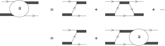
Figure 2: The first few diagrams contributing to $S=3/2$ $nd$-scattering (first line) and the integral equation which sums the diagrams to all orders (second line).

Since the leading piece of all diagrams is of the order $\sim Mg_{T}^{2}/Q^{2}$, they have to be resummed for typical momenta $Q\sim 1/a_{2}^{t}$. This is conveniently achieved by solving the integral equation given by the second line in Fig. 2. Performing the integration over the time component of the four-momentum flowing in the loop and projecting onto the $S$-waves, we obtain the scattering amplitude $a(k,p)$,[17]

$$\frac{3}{4}\left(1/a^{t}_{2}+\sqrt{3p^{2}/4-ME}\right)^{-1}a(p,k)$$ (7)

$$=-K(p,k)-\frac{2}{\pi}\int_{0}^{\infty}\frac{q^{2}\;dq}{q^{2}-k^{2}-i\epsilon}K(p,q)\,a(q,k)\,,$$

where

$$K(p,q)=\frac{1}{2pq}\ln\left(\frac{q^{2}+pq-p^{2}-ME}{q^{2}-pq-p^{2}-ME}\right)\,$$ (8)

and $ME=3k^{2}/4-1/(a^{t}_{2})^{2}$ is the total energy. $k\,(p)$ denote the incoming (outgoing) momenta in the center of mass frame. The amplitude $a(p,k)$ is normalized such that the on-shell value $a(k,k)=(k\cot\delta-ik)^{-1}$ where $\delta$ is the elastic scattering phase shift. The solution of Eq. (7) can be obtained numerically and is very insensitive to the high momentum modes in the integral equation. If, for example, the integral equation is cut off at some finite momentum $\Lambda$, the low energy behavior of the solution remains unchanged. The EFT in this channel is very predictive. The solution of Eq. (7) is shown by the dashed line in Fig. 3.

Figure 3: $k\cot\delta$ for $S=3/2$ $nd$-scattering to order $(r_{2}/a_{2})^{0}$ (dashed line) and $(r_{2}/a_{2})^{2}$ (solid line). The dots [18] and the triangle [19] indicate the experimental values.

When the corrections of the effective range in the two-nucleon interaction are taken into account up to ${\cal O}((r_{2}/a_{2})^{2})$, one obtains the solid curve [20] which agrees nicely with the phase shift analysis of van Oers and Seagrave (dots).[18] For the scattering length the agreement is even better. The calculation to ${\cal O}((r_{2}/a_{2})^{2})$ gives [21] $a_{3}^{(3/2)}=(6.33\pm 0.10)$ fm to be compared with the experimental value [19] $a_{3}^{(3/2)}=(6.35\pm 0.02)$ fm. Furthermore, the EFT expansion in powers of $r_{2}/a_{2}$ converges well, as the contributions from ${\cal O}((r_{2}/a_{2})^{0})$ to ${\cal O}((r_{2}/a_{2})^{2})$ to the scattering length are $a_{3}^{(3/2)}=(5.09+0.91+0.33)$ fm, in order. The extension beyond the deuteron breakup threshold and the inclusion of pions in KSW counting has recently been carried out by Bedaque and Grießhammer.[22]

4 $S=1/2$ $nd$-Scattering and the Triton

In the $S=1/2$ channel, the situation is more complicated. The two-nucleon interactions can now take place both in the ${}^{3}S_{1}$ and ${}^{1}S_{0}$ partial waves. As shown in Fig. 4, there are two coupled amplitudes, $a$ and $b$.

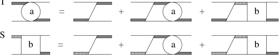
Figure 4: Coupled integral equations for $S=1/2$ $nd$-scattering. $\vec{T}\,(\mbox{\boldmath$S$})$ dibaryon is indicated by grey shaded (black) thick line.

The amplitude $a$ which has both an incoming and outgoing dibaryon field $\vec{T}$ gives the phase shifts for $S=1/2$ $nd$-scattering. However, $a$ is coupled to the amplitude $b$ which has an incoming dibaryon $S$ and an outgoing dibaryon $\vec{T}$. Although only $a$ corresponds to $S=1/2$ $nd$-scattering, both amplitudes have the quantum numbers of the triton. From the Lagrangian, Eq. (2), one obtains the coupled integral equations for the two amplitudes. After the integration over the time component of the loop-momentum and the projection onto the $S$-waves has been carried out, we have

$$\frac{3}{2}\left(1/a_{2}^{t}+\sqrt{3p^{2}/4-ME}\right)^{-1}a(p,k)$$ (9)

$$=K(p,k)+\frac{2}{\pi}\int_{0}^{\Lambda}\frac{q^{2}\;dq}{q^{2}-k^{2}-i\epsilon}K(p,q)[a(q,k)+3b(q,k)]$$

$$2\,\frac{\sqrt{3p^{2}/4-ME}-1/a_{2}^{s}}{p^{2}-k^{2}}\;b(p,k)$$ (10)

$$=3K(p,k)+\frac{2}{\pi}\int_{0}^{\Lambda}\frac{q^{2}\;dq}{q^{2}-k^{2}-i\epsilon}K(p,q)[3a(q,k)+b(q,k)]\,.$$

As before, $k$ ($p$) denote the incoming (outgoing) momenta in the center of mass frame and $ME=3k^{2}/4-(1/a_{2}^{t})^{2}$ is the total energy. The kernel $K(p,q)$ is given in Eq. (8). $a_{2}^{t}$ $(a_{2}^{s})$ are the scattering lengths in the ${}^{3}S_{1}$ $(^{1}S_{0})$ $NN$ channels, respectively. The amplitude $a(p,k)$ is normalized such that $a(k,k)=(k\cot\delta-ik)^{-1}$ with $\delta$ the elastic scattering phase shift in the $S=1/2$ channel. Furthermore, we have introduced a momentum cutoff $\Lambda$ in the integral equations. Eqs. (9, 10) have previously been derived using different methods.[17] In the limit $\Lambda\to\infty$ these equations do not have a unique solution because the phase of the asymptotic solution is undetermined.[23] For a finite $\Lambda$ this phase is fixed and the solution is unique. However, the equations with a cutoff have the same disease as in the boson case: a strong cutoff dependence that does not appear in any order perturbation theory.[12, 13, 14] The amplitude $a(p,k=\mbox{const.})$ shows a strongly oscillating behavior. Varying the cutoff $\Lambda$ slightly changes the asymptotic phase by a number of ${\cal O}(1)$ and results in large changes of the amplitude at the on-shell point $a(p=k)$. This cutoff dependence is not created by divergent Feynman diagrams. It is a nonperturbative effect and appears although all individual diagrams are UV finite.

In order to control this strong $\Lambda$ dependence, it is useful to note that the integral equations (9, 10) are $SU(4)$ symmetric in the ultraviolet (UV). Therefore it is sufficient to consider the $SU(4)$ limit ($a_{2}^{t}=a_{2}^{s}=a_{2}$), since the cutoff dependence is a problem rooted in the UV behavior of the amplitudes. Furthermore, we note that the equations for $a_{+}=[a+b]$ and $a_{-}=[a-b]$ decouple in the $SU(4)$ limit. The equations for $a_{+}$ and $a_{-}$ are given by

$$\frac{3}{4}\left(1/a_{2}+\sqrt{3p^{2}/4-ME}\right)^{-1}a_{+}(p,k)$$ (11)

$$=2K(p,k)+\frac{2H(\Lambda)}{\Lambda^{2}}+\frac{2}{\pi}\int_{0}^{\Lambda}\frac{q^{2}\;dq}{q^{2}-k^{2}-i\epsilon}\left\{2K(p,q)+\frac{2H(\Lambda)}{\Lambda^{2}}\right\}a_{+}(q,k)$$

$$\frac{3}{4}\left(1/a_{2}+\sqrt{3p^{2}/4-ME}\right)^{-1}a_{-}(p,k)$$ (12)

$$=-K(p,k)\vphantom{\frac{1}{2}}-\frac{2}{\pi}\int_{0}^{\Lambda}\frac{q^{2}\;dq}{q^{2}-k^{2}-i\epsilon}K(p,q)\,a_{-}(q,k)\,,$$

where we have introduced a contact three-body force $H(\Lambda)$ which runs with the cutoff $\Lambda$ into the equation for $a_{+}$. Let us disregard the three-body force for a moment. The equation for $a_{+}$ is exactly the same equation as in the case of spinless bosons while the equation for $a_{-}$ is the same equation as in the $S=3/2$ channel. The $S=3/2$ equation is well behaved and its solution is very insensitive to the cutoff as discussed in the previous section. Consequently, the observed cutoff dependence stems solely from the equation for $a_{+}$. As an example, the cutoff dependence of $a_{+}(p,k=0)$ is shown by the solid, dashed, and dash-dotted curves in Fig. 5 for three different cutoffs, $\Lambda=1.0,\,2.0,\,3.0\times 10^{4}a_{2}^{-1}$.

Figure 5: Cutoff dependence of $a_{+}(p,k=0)$. Solid, dashed, and dash-dotted curves are for $H=0$ and $\Lambda=1.0,\,2.0,\,3.0\times 10^{4}a_{2}^{-1}$, respectively. Dotted, short-dash-dotted, and short-dashed curves show the effect of the three-body force for $\Lambda=10^{4}a_{2}^{-1}$ and $H=-6.0,\,-2.5,\,-1.8$, respectively.

But we already know the solution to this problem: a three-body force counterterm that runs with the cutoff $\Lambda$.[13] This is exactly the three-body force we have introduced into Eq. (11). The dotted, short-dash-dotted, and short-dashed curves in Fig. 5 show the effect of the three-body force $H(\Lambda)$ on $a_{+}(p,k=0)$ for $\Lambda=10^{4}a_{2}^{-1}$ and $H=-6.0,\,-2.5,\,-1.8$. It is clearly seen that the variation of $H$ for a constant $\Lambda$ has the same effect on the amplitude as varying the cutoff. Consequently, we can compensate the changes in the asymptotic phase when $\Lambda$ is varied by adjusting the three-body force term appropriately. (A more detailed discussion of the renormalization procedure can be found in Bedaque’s talk.[12])

We can obtain an approximate expression for the running of $H(\Lambda)$ from invariance under the renormalization group. Requiring that the equation for $a_{+}$ does not change its form when the high momentum modes are integrated out, we find

$$H(\Lambda)=-\frac{\sin(s_{0}\ln({\Lambda}/{\Lambda_{\star}})-{\rm arctg}(1/s_{0}))}{\sin(s_{0}\ln({\Lambda}/{\Lambda_{\star}})+{\rm arctg}(1/s_{0}))}\,,$$ (13)

where $s_{0}\approx 1.0064$.[12, 13, 14] $H(\Lambda)$ contains one new dimensionful parameter, $\Lambda_{*}$, which must be determined from experiment. The running of the three-body force $H(\Lambda)$ according to Eq. (13) is shown by the solid line in Fig. 6.

Figure 6: Running of $H(\Lambda)$ for $\Lambda_{*}=0.9\mbox{ fm}^{-1}$: (a) from Eq. (13) (solid line), (b) from numerical solution of Eq. (11) (dots).

The dots are obtained by adjusting $H(\Lambda)$ such that the low energy solution of Eq. (11) remains unchanged when $\Lambda$ is varied. The observed agreement provides a numerical justification for our proceeding. The three-body force is periodic with $H(\Lambda_{n})=H(\Lambda)$ for $\Lambda_{n}=\Lambda\exp(n\pi/s_{0})\approx\Lambda(22.7)^{n}$. Since it enters only in the equation for $a_{+}=a+b$, the three-body force is also $SU(4)$ symmetric.

Formally, the three-body force term in Eq. (11) is obtained by adding

$${\cal L}_{3}=-\frac{2MH(\Lambda)}{\Lambda^{2}}\bigg{(} g_{T}^{2}N^{\dagger}(\vec{T}\cdot\vec{\sigma})^{\dagger}(\vec{T}\cdot\vec{\sigma})N$$

$$+\frac{1}{3}g_{T}g_{S}\left[N^{\dagger}(\vec{T}\cdot\vec{\sigma})^{\dagger}(\mbox{\boldmath$S$}\cdot\mbox{\boldmath$\tau$})N+h.c.\right]$$

$$+g_{S}^{2}N^{\dagger}(\mbox{\boldmath$S$}\cdot\mbox{\boldmath$\tau$})^{\dagger}(\mbox{\boldmath$S$}\cdot\mbox{\boldmath$\tau$})N\bigg{)}\,,$$

to the Lagrangian, Eq. (2). Eq. (4) represents a contact three-body force written in terms of dibaryon and nucleon fields. Via a Gaussian path integration it is equivalent to a true three-nucleon force,

$${\cal L}_{3}= - \frac{2MH(\Lambda)}{\Lambda^{2}}\bigg{(}\,\frac{g_{T}^{4}}{4\Delta_{T}^{2}}\,(N^{T}\tau_{2}\sigma_{k}\sigma_{2}N)^{\dagger}(N^{\dagger}\sigma_{k}\sigma_{l}N)(N^{T}\tau_{2}\sigma_{l}\sigma_{2}N)$$

$$+\frac{1}{3}\frac{g_{T}^{2}}{2\Delta_{T}}\frac{g_{S}^{2}}{2\Delta_{S}}\left[(N^{T}\tau_{2}\sigma_{k}\sigma_{2}N)^{\dagger}(N^{\dagger}\sigma_{k}\tau_{l}N)(N^{T}\sigma_{2}\tau_{l}\tau_{2}N)+h.c.\right]$$

$$+\frac{g_{S}^{4}}{4\Delta_{S}^{2}}\,(N^{T}\sigma_{2}\tau_{k}\tau_{2}N)^{\dagger}(N^{\dagger}\tau_{k}\tau_{l}N)(N^{T}\sigma_{2}\tau_{l}\tau_{2}N)\,\bigg{)}\,.$$

By performing a Fierz rearrangement, it can then be shown that the three terms in Eq. (4) are equivalent. As a consequence, there is only one three-body force which is also $SU(4)$ symmetric. Naive power counting would suggest that the three-nucleon force scales with $1/(Mm_{\pi}^{4})$. The three-body force from Eqs. (4, 4), however, is enhanced by the renormalization group flow by two powers of $a_{2}$. Using Eq. (6), it is found to scale as $a_{2}^{2}/(Mm_{\pi}^{2})$ which makes it leading order.

Recently Mehen, Stewart, and Wise [24] found an approximate $SU(4)$ symmetry in the two-nucleon sector for $1/a_{2}\ll p\ll m_{\pi}$ and also noticed that the only $S$-wave four-nucleon force that can be written down is $SU(4)$ symmetric. Furthermore, there are no contact interactions with more than four nucleons without derivatives because of the Pauli principle. It is also reasonable to assume that the low-energy dynamics of nuclei is dominated by $S$-wave interactions. Therefore our $SU(4)$ symmetric three-body force together with the findings of Mehen et al.[24] gives an explanation for the approximate Wigner $SU(4)$ symmetry in nuclei.[25]

Now we are in the position to solve the full equations for the broken $SU(4)$ case. Introducing the three-body force from above into Eqs. (9, 10), we obtain

$$\frac{3}{2}\left(1/a_{2}^{t}+\sqrt{3p^{2}/4-ME}\right)^{-1}a(p,k)=K(p,k)+\frac{2H(\Lambda)}{\Lambda^{2}}$$ (16)

$$+\frac{2}{\pi}\int_{0}^{\Lambda}\frac{q^{2}\;dq}{q^{2}-k^{2}-i\epsilon}\left[K(p,q)[a(q,k)+3b(q,k)]+\frac{2H(\Lambda)}{\Lambda^{2}}[a(q,k)+b(q,k)]\right]$$

$$2\,\frac{\sqrt{3p^{2}/4-ME}-1/a_{2}^{s}}{p^{2}-k^{2}}\;b(p,k)=3K(p,k)+\frac{2H(\Lambda)}{\Lambda^{2}}$$ (17)

$$+\frac{2}{\pi}\int_{0}^{\Lambda}\frac{q^{2}\;dq}{q^{2}-k^{2}-i\epsilon}\left[K(p,q)[3a(q,k)+b(q,k)]+\frac{2H(\Lambda)}{\Lambda^{2}}[a(q,k)+b(q,k)]\right]\,.$$

We need one three-body datum to fix the three-nucleon force parameter $\Lambda_{*}$. We choose the experimental value for the $S=1/2$ $nd$-scattering length,[19] $a_{3}^{(1/2)}=(0.65\pm 0.04)\mbox{ fm}$ and find $\Lambda_{*}=0.9\mbox{ fm}^{-1}$. (For the special cutoffs with vanishing $H(\Lambda)$, we recover the results of Ref.[26].) Although one three-body datum is needed as input, the EFT has not lost its predictive power. We can still predict (i) the energy dependence of $S=1/2$ $nd$-scattering and (ii) the binding energy of the triton.

The resulting energy dependence of $S=1/2$ $nd$-scattering for three different cutoffs is shown in Fig. 7.

Figure 7: Energy dependence for $S=1/2$ $nd$-scattering with three different cutoffs $\Lambda=1.9,\,6.0,\,11.6\mbox{ fm}^{-1}$ and $\Lambda_{*}=0.9\mbox{ fm}^{-1}$ (hidden under the solid curve). Dashed curve gives estimate of range corrections. Experimental points are from van Oers and Seagrave [18] (dots) and Dilg et al. [19] (triangle).

It is clearly seen that the introduction of the three-body force renders the low-energy amplitude cutoff independent. The scattering length is reproduced exactly because it was used to fix $\Lambda_{*}$. The agreement for finite momentum is at least encouraging. Our experience from the $S=3/2$ channel is that the range corrections improve the agreement considerably (cf. Fig. 3). The dashed curve in Fig. 7 gives a crude estimate of these corrections. In the zero range approximation, we have the relation

$$\sqrt{MB_{2}}=1/a_{2}^{t},$$ (18)

which holds only approximately in nature. In our calculations we take the deuteron binding energy $B_{2}$ from experiment and determine $a_{2}^{t}$ from Eq. (18). The dashed curve in Fig. 7 is obtained by taking the experimental value of $a_{2}^{t}$ as input and leaving all other parameters unchanged. From the estimated size of the range corrections, we anticipate an improved agreement once the range corrections are included. (One should also keep in mind that the experimental phase shift analysis [18] does not give any error estimate).

The triton binding energy is obtained from the solution of the homogeneous equations corresponding to Eqs. (16, 17) for $E=-B_{3}$. We find $B_{3}=8.0$ MeV for the triton binding energy, to be compared with the experimental result $B_{3}^{exp}=8.48$ MeV which is known to very high precision. For a leading order calculation, the agreement is very good. The theory without pions seems to work for triton physics. However, to draw definite conclusions one has to calculate the range corrections for both the energy dependence and the triton binding energy.

In Fig. 8 we show the bound state spectrum as a function of the cutoff $\Lambda$.

Figure 8: Three-nucleon bound state spectrum for $\Lambda_{*}=0.9\mbox{ fm}^{-1}$. The shallowest bound state corresponds to the triton.

The shallowest bound state is the triton. Its binding energy is cutoff independent. However, as $\Lambda$ is increased new deeper bound states appear whenever $H(\Lambda)$ goes through a pole.

Figure 9: Phillips line: $S=1/2$ $nd$ scattering length $a_{3}^{(1/2)}$ as function of the triton binding energy $B_{3}$: EFT to leading order (solid line); potential models (dots); experiment (cross).

These new bound states appear with infinite binding energy directly at the pole. When the cutoff is increased further, their binding energy reduces and becomes cutoff independent as well. The poles of $H(\Lambda)$ can be parametrized as

$$\Lambda_{n}=\underbrace{f(\Lambda_{*}a_{2})}_{{\cal O}(1)}\exp(n\pi/s_{0})a_{2}^{-1}\,.$$ (19)

One counts $n$ bound states for $\Lambda_{n-1}<\Lambda<\Lambda_{n}$. However, only the states between threshold and $\Lambda\sim m_{\pi}\sim 1/r_{2}$ are within the range of the EFT. By solving Eq. (19) for the number of bound states $n$, we then obtain

$$\#_{BS}=\frac{s_{0}}{\pi}\ln\left(\frac{a_{2}}{r_{2}}\right)+{\cal O}(1)\,,$$ (20)

and recover the well-known Efimov effect.[10] In the limit $a_{2}\to\infty$, an infinite number of shallow three-body bound states accumulates at threshold. That these bound states are shallow follows from the fact that the binding energy is naturally given in units of $1/(Ma_{2}^{2})$ which vanishes as $a_{2}\to\infty$. Furthermore, we also recover the Thomas effect.[11] In a hypothetical world where $\Lambda\sim m_{\pi}\sim 1/r_{2}\to\infty$, the range of the EFT increases and deeper and deeper physical bound states appear. Consequently, there is an infinitely deep bound state for $\Lambda\to\infty$. However, for $m_{\pi}\sim 1/r_{2}$ as in the real world the deep bound states are outside the range of the EFT and their presence does not influence the physics of the shallow ones.

Moreover, the variation of the parameter $\Lambda_{*}$ gives a natural explanation for the Phillips line.[9] No matter how good the agreement with the actual experimental number is, values of $B_{3}$ and $a_{3}^{(1/2)}$ in different potential models are correlated and fall on the Phillips line. Obviously, there is a correlation between $B_{3}$ and $a_{3}^{(1/2)}$. In the EFT framework, different models correspond in leading order to different values of $\Lambda_{*}$. Varying $\Lambda_{*}$ then generates the observed Phillips line. The dynamics of QCD chooses a particular value which up to higher order corrections is $\Lambda_{*}=0.9\mbox{ fm}^{-1}$. In Fig. 9 we show the Phillips line obtained in the EFT compared with results from various potential model calculations [27] and the experimental values for $B_{3}$ and $a_{3}^{(1/2)}$. Our Phillips line is slightly below the one from the potential models. We expect this discrepancy to be reduced once range corrections are taken into account.

5 Conclusions

We have studied the three-nucleon system using EFT methods. While for $nd$-scattering in the $S=3/2$ channel precise predictions are obtained in a straightforward way, the $S=1/2$ channel is more complicated. It displays a strong cutoff dependence even though all individual diagrams are UV finite. In this channel a nonperturbative renormalization takes place similar to the case of spinless bosons. This renormalization requires an $SU(4)$ symmetric three-body force which is enhanced to leading order by the renormalization group flow. Together with the recent results of Mehen et al.[24] this gives an explanation for the approximate $SU(4)$ symmetry in nuclei. Furthermore, we find that the Phillips line is a consequence of variations in the new dimensionful parameter $\Lambda_{*}$ which is introduced by the three-body force. $\Lambda_{*}$ is not given from two-nucleon data alone and has to be determined from a three-body datum. In the appropriate limits for the two-body parameters $a_{2}$ and $r_{2}$, we also recover the well known Thomas and Efimov effects.

The leading order of the EFT gives a quantitative description of the triton binding energy and the energy dependence for $S=1/2$ $nd$-scattering. The theory shows the potential for a realistic description of the triton once the range corrections are included. Immediate applications of the EFT include polarization observables in $nd$-scattering and triton properties such as its charge form factor. The incorporation of the long range Coulomb force would widen the possible applications considerably as $pd$-scattering and the physics of ³He becomes accessible.

Finally, since the pionless theory is equivalent to the leading order in KSW counting,[6] the success in the three-nucleon system opens the possibility of applying the EFT method to a large class of systems with three or more nucleons.

References

References

- [1] G.P. Lepage, in From Actions to Answers, TASI’89, ed. T. DeGrand and D. Toussaint (World Scientific, Singapore, 1990); D.B. Kaplan, nucl-th/9506035; H. Georgi, Ann. Rev. Part. Sci. 43, 209 (1994).
- [2] S. Weinberg, Phys. Lett. B 251, 288 (1990); Nucl. Phys. B 363, 3 (1991).
- [3] Nuclear Physics with Effective Field Theory, ed. R. Seki, U. van Kolck, and M.J. Savage (World Scientific, Singapore, 1998)
- [4] U. van Kolck, nucl-th/9902015.
- [5] U. van Kolck, in Proceedings of the Workshop on Chiral Dynamics 1997, Theory and Experiment, ed. A. Bernstein, D. Drechsel, and T. Walcher (Springer-Verlag, Berlin, Heidelberg, 1998); Nucl. Phys. A 645, 273 (1999).
- [6] D.B. Kaplan, M.J. Savage, and M.B. Wise, Phys. Lett. B 424, 390 (1998); Nucl. Phys. B 534, 329 (1998).
-
[7]
J. Gegelia, Phys. Lett. B 429, 227 (1998),
nucl-th/9802038, nucl-th/
9805008. - [8] M.J. Savage, this volume and references therein.
- [9] A.C. Phillips, Nucl. Phys. A 107, 209 (1968).
- [10] V.N. Efimov, Sov. J. Nucl. Phys. 12, 589 (1971); Phys. Rev. C 47, 1876 (1993).
- [11] L.H. Thomas, Phys. Rev. 47, 903 (1935).
- [12] P.F. Bedaque, this volume.
- [13] P.F. Bedaque, H.-W. Hammer, and U. van Kolck, Phys. Rev. Lett. 82, 463 (1999); Nucl. Phys. A 646, 444 (1999).
- [14] H.-W. Hammer, in Proceedings of BARYONS 98 (World Scientific, Singapore, to appear), nucl-th/9811047.
- [15] J.-W. Chen, G. Rupak, and M.J. Savage, nucl-th/9902056.
- [16] D.B. Kaplan, Nucl. Phys. B 494, 471 (1997).
- [17] G.V. Skorniakov and K.A. Ter-Martirosian, Sov. Phys. JETP 4, 648 (1957).
- [18] W.T.H. van Oers and J.D. Seagrave, Phys. Lett. B 24, 562 (1967).
- [19] W. Dilg, L. Koester, and W. Nistler, Phys. Lett. B 36, 208 (1971).
- [20] P.F. Bedaque, H.-W. Hammer, and U. van Kolck, Phys. Rev. C 58, R641 (1998).
- [21] P.F. Bedaque and U. van Kolck, Phys. Lett. B 428, 221 (1998).
- [22] P.F. Bedaque and H.W. Grießhammer, in preparation.
- [23] G.S. Danilov and V.I. Lebedev, Sov. Phys. JETP 17, 1015 (1963); G.S. Danilov, Sov. Phys. JETP 13, 349 (1961).
- [24] T. Mehen, I.W. Stewart, and M. Wise, hep-ph/9902370
- [25] E.P. Wigner, Phys. Rev. 51, 106 (1937).
- [26] V.F. Kharchenko, Sov. J. Nucl. Phys. 16, 173 (1973).
- [27] J.L. Friar, private communication; C.R. Chen, G.L. Payne, J.L. Friar, and B.F. Gibson, Phys. Rev. C 44, 50 (1991).