Isoscalar M1 and E2 Amplitudes in $np\rightarrow d\gamma$  

Abstract

The low energy radiative capture process $np\rightarrow d\gamma$ provides a sensitive probe of the two-nucleon system. The cross section for this process is dominated by the isovector $M1$ amplitude for capture from the ${}^{1}\kern-1.4ptS_{0}$ channel via the isovector magnetic moment of the nucleon. In this work we use effective field theory to compute the isoscalar $M1$ and isoscalar $E2$ amplitudes that are strongly suppressed for cold neutron capture. The actual value of the isoscalar $E2$ amplitude is expected to be within $\sim 15\%$ of the value computed in this work. In contrast, due to the vanishing contribution of the one-body operator at leading order and next-to-leading order, the isoscalar $M1$ amplitude is estimated to have a large uncertainty. We discuss in detail the deuteron quadrupole form factor and ${}^{3}\kern-1.4ptS_{1}-{}^{3}\kern-1.4ptD_{1}$ mixing.

April 1999; Revised August 1999.

The cross section for radiative capture $np\rightarrow d\gamma$ of thermal neutrons has an important place in nuclear physics as it provides a clear demonstration of strong interaction physics that is not constrained by nucleon-nucleon scattering phase shift data alone. Effective range theory[1, 2] uniquely describes the scattering of low-energy nucleons, yet fails to reproduce the measured cross section of $\sigma^{{\rm expt}}=334.2\pm 0.5\ {\rm mb}$ (measured at an incident neutron speed of $\left|{\bf v}\right|=2200$ m/s)[3] for $np\rightarrow d\gamma$ at the $10\%$ level. In the effective field theory appropriate for very low momentum interactions[4] (i.e. without pions), this discrepancy is understood to arise from the omission of a four-nucleon-one-magnetic-photon operator that enters at the same order as effective range contributions. Conventionally, this discrepancy is attributed to pion-exchange-currents[5, 6]. The cross section for $np\rightarrow d\gamma$ at very low energies is dominated by the capture of nucleons in the ${}^{1}\kern-1.4ptS_{0}$ state, via the nucleon isovector magnetic moment, the amplitude for which we denote by $M1_{V}$. This particular amplitude is much larger than other amplitudes for several reasons. First, initial state interactions give a contribution proportional to the large scattering length in the ${}^{1}\kern-1.4ptS_{0}$ channel, $a^{({}^{1}\kern-0.98ptS_{0})}=-23.714\pm 0.013~{}{\rm fm}$. Second, the $M1_{V}$ amplitude is proportional to the nucleon isovector magnetic moment, $\kappa_{1}$, which is much larger than the nucleon isoscalar magnetic moment, $\kappa_{0}$, which dictates the size of the one-body contribution to the isoscalar magnetic amplitude, $M1_{S}$. Third, the capture from the ${}^{3}\kern-1.4ptS_{1}$ channel that does proceed via the nucleon isoscalar magnetic interaction (the one-body contribution) must vanish at zero-momentum transfer as it is the matrix element of the spin operator between orthogonal eigenstates. Finally, the electric amplitudes, $E1_{V}$ for capture from the P-wave and $E2_{S}$ for capture from the ${}^{3}\kern-1.4ptS_{1}$ channel, are suppressed by additional powers of nucleon momentum or photon energy compared to $M1_{V}$.

While the $M1_{S}$, $E2_{S}$ and $E1_{V}$ amplitudes are much smaller than $M1_{V}$, measurements of spin-dependent observables can determine specific combinations of these amplitudes. Two such observables are the circular polarization of photons emitted in the capture of polarized neutrons by unpolarized protons, and the angular distribution of photons emitted in the capture of polarized neutrons by polarized protons. The circular polarization of photons emitted in the forward direction in the capture of polarized neutrons on unpolarized protons has been measured to be[7] $P_{\gamma}^{\rm expt}=-(1.5\pm 0.3)\times 10^{-3}$. This value is consistent with previous theoretical estimates[8]. An experiment that will measure the angular distribution of photons emitted in the capture of polarized neutrons on polarized protons is to be carried out at the ILL reactor facility[9] and results should be available in the near future.

In this work, we calculate the $M1_{S}$ and $E2_{S}$ isoscalar amplitudes that contribute to $np\rightarrow d\gamma$ using the effective field theory (EFT) of nucleon-nucleon interactions without pions, ${\rm EFT}({\pi\hskip-6.00006pt/})$, as detailed in [4], using KSW power counting[19, 21]. A significant amount of progress has been made in the application of EFT to the two- and three-nucleon systems[6][10]-[39] during the past few years. A test of this formalism will be a comparison between these predictions for the strongly suppressed amplitudes in $np\rightarrow d\gamma$ and the measured experimental asymmetries which constrain them. Calculations of these suppressed amplitudes using an alternative power counting are being performed by Park, Kubodera, Min and Rho[40]. Our work results from a challenge issued by M. Rho for the community to make predictions for these amplitudes[40].

The amplitude for low-energy $np\rightarrow d\gamma$ is

$$T = ie\ X_{M1_{V}}\ \varepsilon^{abc}\epsilon_{(d)}^{\ast a}\ {\bf k}^{b}\ \epsilon_{(\gamma)}^{\ast c}\ U^{T}_{\rm n}\tau_{2}\tau_{3}{\bf\sigma}_{2}\ U_{\rm p}\ +\ e\ X_{E1_{V}}\ U^{T}_{\rm n}\ \tau_{2}\tau_{3}\ {\bf\sigma}_{2}\ {\bf\sigma}\cdot\epsilon_{(d)}^{*}\ U_{\rm p}\ {\bf p}\cdot\epsilon_{(\gamma)}^{*}$$ (1)

$$+ e\ X_{M1_{S}}{1\over\sqrt{2}}\ U^{T}_{\rm n}\tau_{2}{\bf\sigma}_{2}\left[{\bf\sigma}\cdot{\bf k}\ \epsilon_{(d)}^{\ast}\cdot\epsilon_{(\gamma)}^{\ast}-\epsilon_{(d)}^{\ast}\cdot{\bf k}\ \epsilon_{(\gamma)}^{\ast}\cdot{\bf\sigma}\right]\ U_{\rm p}$$ (2)

$$+ e\ X_{E2_{S}}{1\over\sqrt{2}}\ U^{T}_{\rm n}\tau_{2}{\bf\sigma}_{2}\left[{\bf\sigma}\cdot{\bf k}\ \epsilon_{(d)}^{\ast}\cdot\epsilon_{(\gamma)}^{\ast}+\epsilon_{(d)}^{\ast}\cdot{\bf k}\ \epsilon_{(\gamma)}^{\ast}\cdot{\bf\sigma}-{\frac{2}{n-1}}\sigma\cdot\epsilon_{(d)}^{\ast}\ {\bf k}\cdot\epsilon_{(\gamma)}^{\ast}\right]\ U_{\rm p}\ \ \ ,$$ (3)

where we have shown only the lowest partial waves, corresponding to electric dipole capture of nucleons in a P-wave with amplitude $X_{E1_{V}}$, isovector magnetic capture of nucleons in the ${}^{1}\kern-1.4ptS_{0}$ channel with amplitude $X_{M1_{V}}$, isoscalar magnetic capture of nucleons in the ${}^{3}\kern-1.4ptS_{1}$ channel with amplitude $X_{M1_{S}}$, and isoscalar electric quadrupole capture of nucleons in the ${}^{3}\kern-1.4ptS_{1}$ channel with amplitude $X_{E2_{S}}$. As we dimensionally regulate the divergences that appear in the effective field theory we keep explicit space-time dependence in the amplitudes shown in eq. (3), with $n$ the number of space-time dimensions. $U_{\rm n}$ is the neutron two-component spinor and $U_{\rm p}$ is the proton two-component spinor. ${\bf p}$ is half the neutron momentum in the proton rest frame, while ${\bf k}$ is the photon momentum. The photon polarization vector is $\epsilon_{(\gamma)}$, and $\epsilon_{(d)}$ is the deuteron polarization vector. For convenience, we define dimensionless variables $\tilde{X}$, by

$$\frac{|{\bf p}|M_{N}}{\gamma^{2}}X_{E1_{V}}\ = i\frac{2}{M_{N}}\sqrt{\frac{\pi}{\gamma^{3}}}\ \tilde{X}_{E1_{V}}\quad,\quad X_{M1_{V}}\ =i\frac{2}{M_{N}}\sqrt{\frac{\pi}{\gamma^{3}}}\ \tilde{X}_{M1_{V}}\quad,\;$$ (4)

$$X_{M1_{S}}\ = i\frac{2}{M_{N}}\sqrt{\frac{\pi}{\gamma^{3}}}\ \tilde{X}_{M1_{S}}\quad,\quad X_{E2_{S}}\ =i\frac{2}{M_{N}}\sqrt{\frac{\pi}{\gamma^{3}}}\ \tilde{X}_{E2_{S}}\quad,$$ (5)

where $\gamma=\sqrt{M_{N}B}\sim 45.6~{}{\rm MeV}$ is the deuteron binding momentum, with $B$ the deuteron binding energy.

By measuring certain observables of the $np\rightarrow d\gamma$ process the four amplitudes $\tilde{X}_{E1_{V}}$, $\tilde{X}_{M1_{V}}$, $\tilde{X}_{M1_{S}}$, and $\tilde{X}_{E2_{S}}$, can be determined or constrained. The simplest quantity to measure is the total cross section for the capture of unpolarized cold neutrons with speed $|{\bf v}|$ by unpolarized protons at rest (the neutron velocity ${\bf v}$ is related to the momentum ${\bf p}$ by ${\bf p}={1\over 2}M_{N}{\bf v}$, where relativistic corrections have been neglected). In terms of the amplitudes given in eq. (3) and eq. (5) the unpolarized cross section is

$$\sigma=\frac{8\pi\alpha\gamma^{3}}{M_{N}^{5}|{\bf v}|}\left[|\tilde{X}_{M1_{V}}|^{2}\ +\ |\tilde{X}_{E1_{V}}|^{2}\ +\ |\tilde{X}_{M1_{S}}|^{2}\ +\ |\tilde{X}_{E2_{S}}|^{2}\right]\ \ \ ,$$ (6)

where $\alpha$ is the fine-structure constant. The cross section for the capture of cold neutrons is dominated by $\tilde{X}_{M1_{V}}$ by several orders of magnitude and therefore a measurement of $\sigma$ does not constrain the other three amplitudes.

A spin-polarized neutron beam incident upon a spin-polarized proton target enables spin-dependent observables to be measured, even without measuring the polarization of the out-going photon or deuteron. If the protons have polarization $\eta_{\rm p}$ and the neutrons have polarization $\eta_{\rm n}$, along the direction of the incident neutron momentum, the spin-dependent capture cross section is

$$I_{\eta_{\rm n}\eta_{\rm p}}(\theta)\ =\ {\frac{d\sigma_{\eta_{\rm n}\eta_{\rm p}}}{d\cos\theta}} = \frac{4\pi\alpha\gamma^{3}}{M_{N}^{5}|{\bf v}|}\left[|\tilde{X}_{M1_{V}}|^{2}(1-\eta_{\rm n}\eta_{\rm p})\ +\ {1\over 2}|\tilde{X}_{E1_{V}}|^{2}\sin^{2}\theta\ (3+\eta_{\rm n}\eta_{\rm p})\right.$$ (10)

$$\left.+\ {1\over 2}|\tilde{X}_{M1_{S}}|^{2}\ (2+\eta_{\rm n}\eta_{\rm p}\ \sin^{2}\theta)+\ {1\over 2}|\tilde{X}_{E2_{S}}|^{2}\ (2+\eta_{\rm n}\eta_{\rm p}\ \sin^{2}\theta)\ \right.$$

$$\left.+\ {\rm Re}\left(\tilde{X}_{M1_{S}}\tilde{X}_{E2_{S}}^{\ast}\right)\eta_{\rm n}\eta_{\rm p}(1-3\cos^{2}\theta)\ \right.$$

$$\left.\ -\ 2\sqrt{2}\ {\rm Re}[\tilde{X}_{E1_{V}}\tilde{X}_{E2_{S}}^{*}]\eta_{\rm n}\eta_{\rm p}\ \cos\theta\sin^{2}\theta\qquad\right]\ \ \ ,$$

where $\theta$ is the angle between the polarization axis and the direction of the emitted photon. Spin-averaging the expression given in eq. (10) over the initial nucleon spin states, $(\eta_{\rm n},\eta_{\rm p})=(\pm 1,\pm 1)$ and integrating over all angles reproduces the spin independent cross section shown in eq. (6). From this one can define the angular asymmetry,

$$S_{\eta_{\rm n}\eta_{\rm p}}(\theta) \ =\ {I_{\eta_{\rm n}\eta_{\rm p}}(\theta)-I_{\eta_{\rm n}\eta_{\rm p}}(0)\over I_{\eta_{\rm n}\eta_{\rm p}}(\theta)+I_{\eta_{\rm n}\eta_{\rm p}}(0)}\ =\ \frac{\sin^{2}\theta}{4(1-\eta_{\rm n}\eta_{\rm p})}\left[S^{(1)}\ +\ \eta_{\rm n}\eta_{\rm p}S^{(2)}\right]\ \ \ ,$$ (11)

where

$$S^{(1)} = {3|\tilde{X}_{E1_{V}}|^{2}\over|\tilde{X}_{M1_{V}}|^{2}}$$ (12)

$$S^{(2)} = {\left(|\tilde{X}_{E1_{V}}|^{2}\ +\ |\tilde{X}_{M1_{S}}|^{2}\ +\ |\tilde{X}_{E2_{S}}|^{2}\ +\ 6{\rm Re}[\tilde{X}_{M1_{S}}\tilde{X}_{E2_{S}}^{*}]\ -\ 4\sqrt{2}{\rm Re}[\tilde{X}_{E1_{V}}\tilde{X}_{E2_{S}}^{*}]\cos\theta\right)\over\ |\tilde{X}_{M1_{V}}|^{2}}\ \ \ \ .$$ (13)

For systems with high polarization, measurement of this angular asymmetry constrains the small amplitudes. In the expressions for $S^{(1)}$ and $S^{(2)}$ that appear in eq. (13) we have neglected the small $M1_{S}$, $E2_{S}$ and $E1_{V}$ amplitudes in the denominators.

If the polarization of the out-going photon can be measured, then other spin-dependent observables can be considered. For a polarized neutron incident upon an unpolarized proton target, there is a different cross section for production of right-handed versus left-handed circularly polarized photons. Defining the asymmetry $A^{\gamma}_{\eta_{\rm n}}(\theta)$ to be the ratio of the difference to the sum of these cross sections,

$$A^{\gamma}_{\eta_{\rm n}}(\theta) = \eta_{\rm n}\left[\ \left(P_{\gamma}(M1)\ +\ P_{\gamma}(E2)\right)\ \cos\theta\ +\ P_{\gamma}(E1)\ \sin^{2}\theta\right]\ \ \ ,$$ (14)

where

$$P_{\gamma}(M1) = {\sqrt{2}{\rm Re}[\tilde{X}_{M1_{V}}\tilde{X}_{M1_{S}}^{*}]\over|\tilde{X}_{M1_{V}}|^{2}}\ \ \ ,\ \ \ P_{\gamma}(E2)\ =\ {\sqrt{2}{\rm Re}[\tilde{X}_{M1_{V}}\tilde{X}_{E2_{S}}^{*}]\over|\tilde{X}_{M1_{V}}|^{2}}\ \ ,$$ (15)

$$P_{\gamma}(E1) = {{\rm Re}[\tilde{X}_{M1_{V}}\tilde{X}_{E1_{V}}^{*}]\over|\tilde{X}_{M1_{V}}|^{2}}\ \ \ ,$$ (16)

where we have again neglected the small $M1_{S}$, $E2_{S}$ and $E1_{V}$ amplitudes in the denominators.

The four amplitudes $\tilde{X}_{E1_{V}}$, $\tilde{X}_{M1_{V}}$, $\tilde{X}_{M1_{S}}$, and $\tilde{X}_{E2_{S}}$, can be computed with ${\rm EFT}({\pi\hskip-6.00006pt/})$. Power counting the leading order (LO) versus next-to-leading order (NLO) for a given amplitude is straightforward and follows the well known power counting rules[4, 19, 21]. However, power counting amplitudes relative to each other is not so straightforward. The reason for this is that there are two different kinematic scales for the capture of cold or thermal neutrons – the photon energy and the momentum of the incident neutron. While the velocity of the incident neutron is always assumed to be small, its finite value gives rise to an $E1_{V}$ amplitude, which for $|{\bf v}|=2200~{}{\rm m/s}$ is comparable to the subleading $M1_{S}$ and $E2_{S}$ amplitudes.

It is convenient to express the $\tilde{X}$ amplitudes as a series in powers of $Q$; $\tilde{X}=\tilde{X}^{(-1)}+\tilde{X}^{(0)}+\tilde{X}^{(1)}+\cdots$ where $Q\sim\gamma/m_{\pi}$ is the small expansion parameter in the theory and superscripts denote the order in $Q$. The isovector $M1$ amplitude $\tilde{X}_{M1_{V}}$ has been computed with EFT previously[4, 26] up to NLO. The amplitude starts at $Q^{0}$ in the power counting,

$$\tilde{X}_{M1_{V}}^{(0)}=\kappa_{1}\left(1-a^{({}^{1}\kern-0.98ptS_{0})}\gamma\right)\quad,$$ (17)

where $\kappa_{1}=(\kappa_{p}-\kappa_{n})/2$ is the isovector nucleon magnetic moment in nuclear magnetons, with $\kappa_{p}=2.79285$, $\kappa_{n}=-1.91304$. While naively, $\tilde{X}_{M1_{V}}^{(0)}$ is of order $Q^{0}$, numerically $\tilde{X}_{M1_{V}}^{(0)}\sim 20$ due to the large numerical values of both $\kappa_{1}$ and $a^{({}^{1}\kern-0.98ptS_{0})}$.

At order $Q^{1}$ there are contributions to $\tilde{X}_{M1_{V}}$ from insertions of the effective range parameter and also contributions from a four-nucleon-one-magnetic operator, described by the Lagrange density

$${\cal L} = e\ {{}^{\pi\hskip-2.625pt/}\hskip-1.99997ptL_{1}}\ \left(N^{T}P_{i}N\right)^{\dagger}\left(N^{T}\overline{P}_{3}N\right){\bf B}_{i}\ +\ {\rm h.c.}\ \ \ ,$$ (18)

where ${\bf B}=\nabla\times{\bf A}$ is the magnetic field operator. $P_{i}$ and $\overline{P}_{i}$ are the ${}^{3}\kern-1.4ptS_{1}$ and ${}^{1}\kern-1.4ptS_{0}$ spin-isospin projection operators respectively, with

$$P_{i}=\frac{1}{\sqrt{8}}\sigma_{2}\sigma_{i}\ \tau_{2}\quad,\quad\overline{P}_{i}=\frac{1}{\sqrt{8}}\sigma_{2}\ \tau_{2}\tau_{i}\quad.$$ (19)

The NLO contribution to the amplitude is found to be[4, 26]

$$\tilde{X}_{M1_{V}}^{(1)} = \ {1\over 2}\kappa_{1}\rho_{d}\gamma\left(1-a^{({}^{1}\kern-0.98ptS_{0})}\gamma\right)$$ (21)

$$-{\displaystyle{M_{N}a^{({}^{1}\kern-0.98ptS_{0})}\gamma^{2}\over 4\pi}}\ (\mu-\gamma)(\mu-\frac{1}{a^{({}^{1}\kern-0.98ptS_{0})}})\left[{{}^{\pi\hskip-2.625pt/}\hskip-1.99997ptL_{1}}-{\displaystyle{\kappa_{1}\pi\over M_{N}}}\left({\displaystyle{r_{0}^{({}^{1}\kern-0.98ptS_{0})}\over\left(\mu-\frac{1}{a^{({}^{1}\kern-0.7ptS_{0})}}\right)^{2}}}+{\displaystyle{\rho_{d}\over(\mu-\gamma)^{2}}}\right)\right]\hskip 1.42271pt\quad,$$

where $r_{0}=2.73\pm 0.03$ fm is the effective range in the ${}^{1}\kern-1.4ptS_{0}$ channel and $\rho_{d}=1.764$ fm is effective range in the ${}^{3}\kern-1.4ptS_{1}$ channel. $\mu$ is the renormalization scale, and the $\mu$-dependence of ${{}^{\pi\hskip-2.625pt/}\hskip-1.99997ptL_{1}}$ yields a renormalization scale independent amplitude, by construction[4, 26]. For convenience we choose $\mu=m_{\pi}$. As $\tilde{X}_{M1_{V}}$ is the dominant amplitude for the capture process, ${{}^{\pi\hskip-2.625pt/}\hskip-1.99997ptL_{1}}=7.24~{}{\rm fm^{4}}$ from the unpolarized cross section [4] in eq. (6).

The cross section for any finite incident nucleon momentum has a contribution from isovector $E1$ capture. Recently, a N³LO calculation of this amplitude has been performed[41] for non-zero energy capture. At N³LO there are contributions from the effective range parameter and from P-wave initial-state interactions which are found to be small. Neglecting the P-wave initial-state interactions, the amplitude is found to be, up to N³LO

$$\tilde{X}_{E1_{V}} = -\frac{|{\bf p}|M_{N}}{\gamma^{2}}\left(1+{1\over 2}\gamma\rho_{d}+{3\over 8}\gamma^{2}\rho_{d}^{2}+{5\over 16}\gamma^{3}\rho_{d}^{3}\right)\ \ \ .$$ (22)

Capture from the P-wave introduces the factor of the external nucleon momentum, $|{\bf p}|$, forcing the amplitude to vanish at threshold. The powers of $\gamma\rho_{d}$ that appears in the amplitude are consistent with the deuteron S-wave normalization factor $1/\sqrt{1-\gamma\rho_{d}}$ that arises in effective range theory. For moderate incident momenta, where $|{\bf p}|\sim Q$, the LO $E1_{V}$ amplitude is of order $Q^{-1}$, and dominates the isovector $M1_{V}$ amplitude, which starts at $Q^{0}$. However, for smaller incident momentum, the $E1_{V}$ amplitude becomes less important. If we take $|{\bf p}|\sim Q^{2}$, the $E1_{V}$ and $M1_{V}$ amplitudes are of the same order in the counting, however, for the neutron incident velocity of $2200~{}{\rm m/s}$, numerically $|{\bf p}|\sim Q^{4}$.

In the zero recoil limit, the matrix element of the nucleon magnetic moment operator between the deuteron and nucleons in the ${}^{3}\kern-1.4ptS_{1}$ channel, contributing to $M1_{S}$, is the matrix element of the spin operator between orthogonal eigenstates states of the strong interaction and thus vanishes. This leads to $\tilde{X}_{M1_{S}}^{(0)}=0$ at LO ($Q^{0}$) and further, the contribution from the one-body operator at NLO ($Q^{1}$) also vanishes. However, at NLO there is a contribution from a four-nucleon-one-photon two-body operator defined by the Lagrange density[4, 21]

$${\cal L} = -e\ {{}^{\pi\hskip-2.625pt/}\hskip-1.99997ptL_{2}}\ i\epsilon_{ijk}\left(N^{T}P_{i}N\right)^{\dagger}\left(N^{T}P_{j}N\right){\bf B}_{k}+\text{h.c.}\ \ \ .$$ (23)

At NLO the deuteron magnetic moment is found to be[21]

$$\mu_{M} = {e\over 2M_{N}}\left(\kappa_{p}\ +\ \kappa_{n}\ +\ {{}^{\pi\hskip-2.625pt/}\hskip-1.99997ptL_{2}}\ {2M_{N}\gamma(\mu-\gamma)^{2}\over\pi}\right)\ \ \ .$$ (24)

Reproducing the experimentally observed value of the deuteron magnetic moment requires that, at this order[4, 21], ${{}^{\pi\hskip-2.625pt/}\hskip-1.99997ptL_{2}}(m_{\pi})=-0.149\text{ fm}^{4}$, which is significantly smaller than the naively estimated size of $\sim 1$ fm⁴. This two-body interaction contributes to $\tilde{X}_{M1_{S}}^{(1)}$, and at NLO we find

$$\tilde{X}_{M1_{S}}^{(1)}=\sqrt{2}\ {\displaystyle{M_{N}\gamma\over 2\pi}}\hskip 1.42271pt{{}^{\pi\hskip-2.625pt/}\hskip-1.99997ptL_{2}}(\mu-\gamma)^{2}\quad.$$ (25)

While formally the leading contribution, the smallness of ${{}^{\pi\hskip-2.625pt/}\hskip-1.99997ptL_{2}}$ suggests that the contribution given in eq. (25) might not dominate over higher order terms, and the $M1_{S}$ amplitude might not be predicted well by ${\rm EFT}({\pi\hskip-6.00006pt/})$ at this order.

To make this more concrete, one can imagine a higher dimension four-nucleon-one-photon local operator that gives rise to a contribution of the form

$$\Delta\tilde{X}_{M1_{S}} \sim \sqrt{2}{\displaystyle{M_{N}\over 2\pi}}\ {{}^{\pi\hskip-2.625pt/}\hskip-1.99997ptL_{X}}\ (\mu-\gamma)^{3}\ \left[(p^{2}+\gamma^{2})+(p^{\prime 2}+\gamma^{2})\right]\ \ \ ,$$ (26)

between states with nucleon momentum $p$ and $p^{\prime}$, since ${{}^{\pi\hskip-2.625pt/}\hskip-1.99997ptL_{X}}\sim(\mu-\gamma)^{-3}$. This object makes a vanishing contribution to the magnetic moment of the deuteron, while making a non-zero contribution to the rate for capture from the ${}^{3}\kern-1.4ptS_{1}$ channel

$$\Delta\tilde{X}_{M1_{S}} \sim \sqrt{2}{\displaystyle{M_{N}\gamma^{2}\over 2\pi}}\ {{}^{\pi\hskip-2.625pt/}\hskip-1.99997ptL_{X}}\ (\mu-\gamma)^{3}\ \ \ \ .$$ (27)

One naively expects ${{}^{\pi\hskip-2.625pt/}\hskip-1.99997ptL_{X}}\sim 1~{}{\rm fm^{6}}$, which would make such a contribution approximately $60\%$ of the amplitude in eq. (25). This relatively large uncertainty in the $M1_{S}$ matrix element is consistent with previous calculations of this quantity[7], and particularly the most recent (preliminary) work of Park, Kubodera, Min and Rho[40], where they find that different treatments of the short-range component of the interaction leads to an approximate $60\%$ uncertainty. At higher orders, there is a contribution from the one-body operator due to the finite energy release of the capture process. Naively, this contribution is much smaller than the expected contribution from higher dimension operators, as estimated in eq. (27), and so we do not consider it further.

The $E2_{S}$ amplitude is dominated by local operators that convert ${}^{3}\kern-1.4ptS_{1}$ states to ${}^{3}\kern-1.4ptD_{1}$ states and vice versa. However, the relatively slow convergence in this channel requires that the calculation be performed to higher orders so that a meaningful estimate of uncertainties is possible. In previous works[4] the deuteron quadrupole form factor and the ${}^{3}\kern-1.4ptS_{1}-{}^{3}\kern-1.4ptD_{1}$ mixing parameter $\overline{\varepsilon}_{1}$[42, 43] were computed up to NLO. Presently, we compute $\overline{\varepsilon}_{1}$ up to N³LO, the deuteron quadrupole form factor up to N²LO and the isoscalar amplitude in $np\rightarrow d\gamma$ up to N²LO.

The lagrange density describing such interaction is [4]

$${\cal L}^{(sd)} = -{\cal T}^{(sd)}_{ij,xy}\left({{}^{\pi\hskip-2.625pt/}\hskip-1.99997ptC_{0}^{(sd)}}\left[P^{i}\right]^{\dagger}\left[{\cal O}^{xy,j}_{2}\right]+{{}^{\pi\hskip-2.625pt/}\hskip-1.99997ptC_{2}^{(sd)}}\left[{\cal O}^{ll,i}_{2}\right]^{\dagger}\left[{\cal O}^{xy,j}_{2}\right]+{{}^{\pi\hskip-2.625pt/}\hskip-1.99997pt\tilde{C}_{2}^{(sd)}}\left[P^{i}\right]^{\dagger}\left[{\cal O}^{mm,xy,j}_{4}\right]\right.$$ (30)

$$\left.+{{}^{\pi\hskip-2.625pt/}\hskip-1.99997ptC_{4}^{(sd)}}\left[{\cal O}^{mm,ll,i}_{4}\right]^{\dagger}\left[{\cal O}^{xy,j}_{2}\right]+{{}^{\pi\hskip-2.625pt/}\hskip-1.99997pt\tilde{C}_{4}^{(sd)}}\left[{\cal O}^{ll,i}_{2}\right]^{\dagger}\left[{\cal O}^{mm,xy,j}_{4}\right]+{{}^{\pi\hskip-2.625pt/}\hskip-1.99997pt{\tilde{\tilde{C}}}_{4}^{(sd)}}\left[P^{i}\right]^{\dagger}\left[{\cal O}^{aa,mm,xy,j}_{6}\right]\right)$$

$$\ +\ ...\ \ \ +\ {\rm h.c.}\ \ \ ,$$

where

$$\left[{\cal O}\right] \equiv \left(N^{T}{\cal O}N\right)\ \ \ ,\ \ \ {\cal T}^{(sd)}_{ij,xy}\ =\ \left(\delta_{ix}\delta_{jy}-{1\over n-1}\delta_{ij}\delta_{xy}\right)$$ (31)

$${\cal O}^{xy,j}_{2} = -{1\over 4}\left(\overleftarrow{\bf D}^{x}\overleftarrow{\bf D}^{y}P^{j}+P^{j}\overrightarrow{\bf D}^{x}\overrightarrow{\bf D}^{y}-\overleftarrow{\bf D}^{x}P^{j}\overrightarrow{\bf D}^{y}-\overleftarrow{\bf D}^{y}P^{j}\overrightarrow{\bf D}^{x}\right)$$ (32)

$${\cal O}^{wz,xy,j}_{4} = {1\over 16}\left(\overleftarrow{\bf D}^{w}\overleftarrow{\bf D}^{z}{\cal O}^{xy,j}_{2}+{\cal O}^{xy,j}_{2}\overrightarrow{\bf D}^{w}\overrightarrow{\bf D}^{z}-\overleftarrow{\bf D}^{w}{\cal O}^{xy,j}_{2}\overrightarrow{\bf D}^{z}-\overleftarrow{\bf D}^{z}{\cal O}^{xy,j}_{2}\overrightarrow{\bf D}^{w}\right)$$ (33)

$${\cal O}^{ab,wz,xy,j}_{6} = -{1\over 64}\left(\overleftarrow{\bf D}^{a}\overleftarrow{\bf D}^{b}{\cal O}^{wz,xy,j}_{4}+{\cal O}^{xy,j}_{2}\overrightarrow{\bf D}^{a}\overrightarrow{\bf D}^{b}-\overleftarrow{\bf D}^{a}{\cal O}^{wz,xy,j}_{4}\overrightarrow{\bf D}^{b}-\overleftarrow{\bf D}^{b}{\cal O}^{wz,xy,j}_{4}\overrightarrow{\bf D}^{a}\right)\ \ \ .$$ (34)

We have not shown higher dimension operators, such as those corresponding to ${\cal O}(p^{8})$, but it is obvious how to include them and what the notation is. The tree-level amplitude for an ${}^{3}\kern-1.4ptS_{1}\rightarrow{}^{3}\kern-1.4ptD_{1}$ transition resulting from this Lagrange density is (in momentum space)

$${\cal A}^{\rm tree}_{sd} = -\left({{}^{\pi\hskip-2.625pt/}\hskip-1.99997ptC_{0}^{(sd)}}+\left[{{}^{\pi\hskip-2.625pt/}\hskip-1.99997ptC_{2}^{(sd)}}+{{}^{\pi\hskip-2.625pt/}\hskip-1.99997pt\tilde{C}_{2}^{(sd)}}\right]p^{2}+\left[{{}^{\pi\hskip-2.625pt/}\hskip-1.99997ptC_{4}^{(sd)}}+{{}^{\pi\hskip-2.625pt/}\hskip-1.99997pt\tilde{C}_{4}^{(sd)}}+{{}^{\pi\hskip-2.625pt/}\hskip-1.99997pt{\tilde{\tilde{C}}}_{4}^{(sd)}}\right]p^{4}\ +\ ...\right)$$ (36)

$$\left[p^{i}p^{j}-{1\over n-1}p^{2}\delta^{ij}\right]\ \ \ .$$

The coefficients that appear in eq. (30) themselves have an expansion in powers of $Q$, e.g. ${{}^{\pi\hskip-2.625pt/}\hskip-1.99997ptC_{0}^{(sd)}}={{}^{\pi\hskip-2.625pt/}\hskip-1.99997ptC_{0,-1}^{(sd)}}+{{}^{\pi\hskip-2.625pt/}\hskip-1.99997ptC_{0,0}^{(sd)}}+...$.

In order to calculate the ${}^{3}\kern-1.4ptS_{1}-{}^{3}\kern-1.4ptD_{1}$ mixing parameter $\overline{\varepsilon}_{1}$ up to N³LO we only require one insertion of ${\cal A}^{\rm tree}_{sd}$, dressed with the appropriate ${}^{3}\kern-1.4ptS_{1}-{}^{3}\kern-1.4ptS_{1}$ interactions. The expression for $\overline{\varepsilon}_{1}$ is straightforward but long and so we do not present it here. We define the coefficients that arise in the momentum expansion of $\overline{\varepsilon}_{1}$, $E_{1}^{(2)}$ and $E_{1}^{(4)}$, by

$$\overline{\varepsilon}_{1} = E_{1}^{(2)}{p^{3}\over\sqrt{p^{2}+\gamma^{2}}}\ +\ E_{1}^{(4)}{p^{5}\over\sqrt{p^{2}+\gamma^{2}}}\ +\ ....$$ (37)

The coefficients are fit to the Nijmegen partial wave analysis[43], and are found to be $E_{1}^{(2)}=0.386\ {\rm fm^{2}}$ and $E_{1}^{(4)}\ =\ -2.800\ {\rm fm^{4}}$. As far as the power counting is concerned it is important to note that the coefficients $E_{1}^{(2)}$ and $E_{1}^{(4)}$ are set by physics at the high scale and therefore are $Q^{0}$ or higher. Thus, contributions of order $Q^{-l}$ must identically vanish[44]. The superscript on the $E_{1}^{(n)\ \prime}s$ denotes the lowest order in $Q$ at which contributions may arise. These conditions ensure non-trivial relations between the coefficients in eq. (30) as the renormalization scale is reduced below the high scale. Each of the coefficients in eq. (30) can be written in terms of physical observables, such as $E_{1}^{(2)}$, $E_{1}^{(4)}$, $\rho_{d}$, $\gamma$, and the renormalization scale $\mu$.

We are free to choose parameters other than the $E_{1}^{(n)\ \prime}s$ to expand in. A quantity that is more directly related to the properties of the deuteron, is $\eta_{sd}$, (written in terms of the ${}^{3}\kern-1.4ptS_{1}-{}^{3}\kern-1.4ptD_{1}$ mixing angle in the Blatt and Biedenharn parameterization of the S-matrix[45]) which is defined to be

$$\eta_{sd} = -\tan\left(\varepsilon_{1}\right)\ \ \ ,\ \ \ \tan\left(2\varepsilon_{1}\right)\ =\ {\tan\left(2\overline{\varepsilon}_{1}\right)\over\sin\left(\overline{\delta}_{0}-\overline{\delta}_{2}\right)}\ \ \ ,$$ (38)

evaluated at the deuteron pole, $|{\bf p}|=i\gamma$. The difference between using $\{\eta_{sd},E_{1}^{(4)}\}$ and $\{E_{1}^{(2)},E_{1}^{(4)}\}$ is higher order in the expansion. In terms of the coefficients $E_{1}^{(2)}$ and $E_{1}^{(4)}$ it is easy to show that, up to N³LO

$$\eta_{sd} = \gamma^{2}\left[E_{1}^{(2)}\left(1-{1\over 2}\gamma\rho_{d}-{1\over 8}\gamma^{2}\rho_{d}^{2}-{1\over 16}\gamma^{3}\rho_{d}^{3}\right)-E_{1}^{(4)}\gamma^{2}\left(1-{1\over 2}\gamma\rho_{d}\right)\right]\ \ \ ,$$ (39)

which is, order by order, $\eta_{sd}=0.0207-0.0042+0.0076-0.0017\ +\ ...\ \ .$ Numerically, it is clear that the expansion is converging, but slowly due to the relatively large size of $E_{1}^{(4)}$ compared to $E_{1}^{(2)}$. This slow convergence will give rise to slow convergence in observables involving the deuteron and therefore it is convenient to invert this relation and use the very precise[43] determination of $\eta_{sd}=0.02543\pm 0.00007$ as one of the expansion parameters.

At LO in ${\rm EFT}({\pi\hskip-6.00006pt/})$ the deuteron quadrupole moment is given entirely in terms of $\eta_{sd}$

$$\mu_{\cal Q}^{(LO)} = {\eta_{sd}\over\sqrt{2}\gamma^{2}}\ =\ 0.335\ {\rm fm^{2}}\ \ \ .$$ (40)

At NLO the four-nucleon-one-photon operator[4] with coefficient ${{}^{\pi\hskip-2.625pt/}\hskip-1.99997ptC_{\cal Q}}$ defined by the Lagrange density

$${\cal L} = {e\ {{}^{\pi\hskip-2.625pt/}\hskip-1.99997ptC_{\cal Q}}\over 2}\ \left(N^{T}P_{i}N\right)^{\dagger}\left(N^{T}P_{j}N\right)\left[\nabla^{i}{\bf E}^{j}\ +\ \nabla^{j}{\bf E}^{i}\ -\ {2\over n-1}\delta^{ij}\ \nabla\cdot{\bf E}\right]$$ (41)

$$= -e\ {{}^{\pi\hskip-2.625pt/}\hskip-1.99997ptC_{\cal Q}}\ \left(N^{T}P_{i}N\right)^{\dagger}\left(N^{T}P_{j}N\right)\left(\nabla^{i}\nabla^{j}-\frac{1}{n-1}\nabla^{2}\delta^{ij}\right)A^{0}\ +\ ....\ \ \ ,$$ (42)

where ${\bf E}$ is the electric field operator, contributes to the deuteron electric quadrupole moment as well as to the isoscalar E2 amplitude in $np\rightarrow d\gamma$. The counterterm is determined by fitting the NLO amplitude to the observed quadrupole moment, and it is convenient to define the quantity $\delta\mu_{\cal Q}$

$$\delta\mu_{\cal Q} = \mu_{\cal Q}^{\rm expt.}-\mu_{\cal Q}^{(LO)}\ =\ -0.0492\ {\rm fm^{2}}\ \ \ ,$$ (43)

which is taken to scale as $Q^{1}$ in the power counting. Solving for the quadrupole counterterm, one finds

$${{}^{\pi\hskip-2.625pt/}\hskip-1.99997ptC_{\cal Q}} = \pi{\sqrt{2}\ \eta_{sd}\ \rho_{d}-2\ \delta\mu_{\cal Q}\ \gamma\over 2\gamma^{2}(\mu-\gamma)^{2}}\ \ \ .$$ (44)

Naively, higher order quadrupole counterterms contribute to the quadrupole form factor and quadrupole moment at N²LO. However, an RG analysis of such contribution shows that they first contribute at N³LO, and we can neglect them in our analysis. Explicit calculation of the deuteron quadrupole form factor[21, 4] up to N²LO gives (neglecting relativistic corrections that are suppressed by additional factors of $m_{\pi}^{2}/M_{N}^{2}$)

$${1\over M_{d}^{2}}F_{\cal Q}(|{\bf k}|) = \delta\mu_{\cal Q}-{3\eta_{sd}\over 2\sqrt{2}\gamma|{\bf k}|^{3}}\left[\ 4|{\bf k}|\left(\gamma\left(1+\gamma\rho_{d}+\gamma^{2}\rho_{d}^{2}\right)+{1\over 6}|{\bf k}|^{2}\rho_{d}\left(1+\gamma\rho_{d}\right)-{1\over 6}\gamma r_{N}^{2}|{\bf k}|^{2}\right)\right.$$ (46)

$$\left.\qquad\qquad\qquad-\left(3|{\bf k}|^{2}+16\gamma^{2}\right)\left(\left(1+\gamma\rho_{d}+\gamma^{2}\rho_{d}^{2}\right)-{1\over 6}r_{N}^{2}|{\bf k}|^{2}\right)\tan^{-1}\left({|{\bf k}|\over 4\gamma}\right)\ \right]\ \ \ ,$$

and the deuteron quadrupole moment, $\mu_{Q}=F_{\cal Q}(0)/M_{d}^{2}$, is reproduced straightforwardly. $r_{N}=0.79\ {\rm fm}$ is the isoscalar nucleon charge radius that first enters at N²LO. It is clear that up to N²LO the quadrupole form factor has a well behaved expansion in powers of $\gamma\rho_{d}$. The overall normalization is largely determined by $\eta_{sd}$, with the counterterm appearing at NLO required to reproduce the quadrupole moment[4]. It is interesting to note that even at N²LO there is no contribution from $E_{1}^{(4)}$, and the form factor is given entirely in terms of $\eta_{sd}$ $\gamma$, $\rho_{d}$ and $\delta\mu_{\cal Q}$. A plot of the quadrupole form factor at LO, NLO and N²LO can be found in fig. (1).

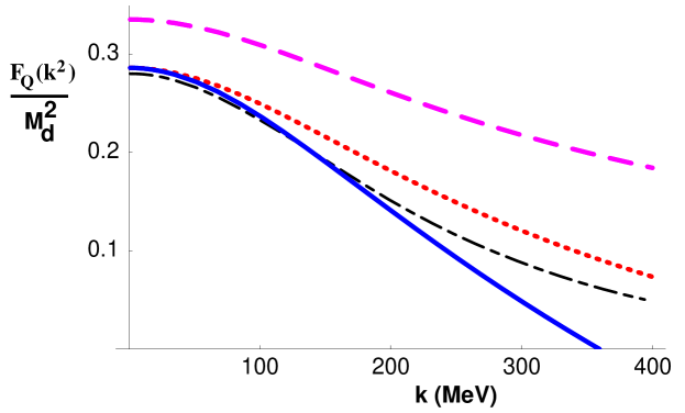
FIG. 1.: The deuteron quadrupole form factor. The dashed, dotted and solid curves denote the LO, NLO and N²LO deuteron quadrupole form factors computed in ${\rm EFT}({\pi\hskip-6.00006pt/})$. The dot-dashed curve corresponds to a calculation with the Bonn-B potential in the formulation of [46] .

Using the above analysis we are in a position to make a prediction for the isoscalar amplitude in $np\rightarrow d\gamma$ up to N²LO. The LO, NLO and N²LO contributions to $\tilde{X}_{E2_{S}}$ are

$$\tilde{X}_{E2_{S}}^{(LO)} = -{1\over 10}\ \eta_{sd}\ \ =\ \ -2.54\times 10^{-3}$$ (47)

$$\tilde{X}_{E2_{S}}^{(NLO)} = -{3\gamma\rho_{d}\over 80}\ \eta_{sd}\ +\ {\gamma^{2}\over 4\sqrt{2}}\ \delta\mu_{\cal Q}\ \ =\ \ -0.86\times 10^{-3}$$ (48)

$$\tilde{X}_{E2_{S}}^{(N^{2}LO)} = -{\gamma^{2}\rho_{d}^{2}\over 64}\ \eta_{sd}\ +\ {3\gamma^{4}\over 40}\ E_{1}^{(4)}\ \ =\ \ -0.67\times 10^{-3}\ \ \ .$$ (49)

It is clear that the perturbative expansion is converging, however, the ratio of the third to second term in the expansion is not particularly small. This suggests that a N³LO calculation is required before one has confidence in the value of this amplitude. A conservative estimate of the uncertainty in the N²LO calculation is the size of the N²LO contribution itself.

Numerically, the ${\rm EFT}({\pi\hskip-6.00006pt/})$ calculations of the subleading amplitudes for near threshold $np\rightarrow d\gamma$ capture are

$$\frac{\tilde{X}_{M1_{S}}}{\tilde{X}_{M1_{V}}}=-5.0\times 10^{-4}\qquad\qquad,\qquad\qquad\frac{\tilde{X}_{E2_{S}}}{\tilde{X}_{M1_{V}}}\ =\ -2.5\times 10^{-4}$$ (50)

with uncertainties that we naively estimate to be of order $\sim 60\%$ and $\sim 15\%$ respectively, due to the omission of higher order terms. For an incident neutron speed of $\left|{\bf v}\right|~{}{\rm m/s}$ in the proton rest frame, we find

$$\frac{\tilde{X}_{E1_{V}}}{\tilde{X}_{M1_{V}}}\ =\ -1.2\times 10^{-4}\ \left({|{\bf v}|\over 2200}\right)\quad,$$ (51)

with an uncertainty that we estimate to be of order $\sim 3\%$[41]. Even for neutrons with $\left|{\bf v}\right|=2200~{}{\rm m/s}$ the $E1_{V}$ capture cross section is comparable to the suppressed amplitudes for $M1_{S}$ and $E2_{S}$ capture.

Using these amplitudes to compute the photon polarizations $P_{\gamma}$, we find

$$P_{\gamma}(M1) = -7.1\times 10^{-4}\ \ \ ,\ \ \ P_{\gamma}(E2)\ =\ -3.5\times 10^{-4}\ \ \ ,$$ (52)

giving a total of $P_{\gamma}=-1.06\times 10^{-3}$ in the forward direction, approximately $2/3$ of the experimentally determined value of[7] $P_{\gamma}^{\rm expt}=-(1.5\pm 0.3)\times 10^{-3}$. Given the large uncertainty in the calculation of the $M1_{S}$ amplitude, and the uncertainty of the measurement, the two are consistent at the order to which we have calculated. Our value of $P_{\gamma}(M1)=-7.1\times 10^{-4}$ is in complete agreement with the results of Burichenko and Kriplovich[8] of $P_{\gamma}(M1)=-7.0\times 10^{-4}$ from a Reid soft-core calculation, but is somewhat less than their zero-range calculation of $P_{\gamma}(M1)=-9.2\times 10^{-4}$. However, given the large uncertainty in our $M1_{S}$ amplitude, both values are consistent. Our value of $P_{\gamma}(E2)=-3.5\times 10^{-4}$ agrees well with the recent calculation of Park, Kubodera, Min and Rho[40], and lies somewhere between the zero-range approximation calculation of $P_{\gamma}(E2)=-2.4\times 10^{-4}$ (which we reproduce at LO in ${\rm EFT}({\pi\hskip-6.00006pt/})$) and Reid soft-core calculation of $P_{\gamma}(E2)=-3.7\times 10^{-4}$ by Burichenko and Kriplovich[8].

The power of effective field theory is that there are well-defined expansion parameters, even when loop graphs appear. It is therefore natural to understand the power counting of the spin-dependent asymmetries that we have considered. The $M1_{S}$ amplitude starts at order $Q^{0}$, but receives its first non-zero contribution at order $Q^{1}$. We have only computed the order $Q^{1}$ contribution. In contrast, the $E2_{S}$ amplitude starts at order $Q^{2}$ and we have computed the order $Q^{2}$, $Q^{3}$ and $Q^{4}$ contributions. Therefore, the observable $P_{\gamma}$ has been computed only to order $Q^{1}$, despite our calculation of part of the order $Q^{2}$, $Q^{3}$ and $Q^{4}$ contributions from the $E2_{S}$ amplitude. This is apparent in the size of the uncertainty arising from higher order terms in the $M1_{S}$ amplitude, that we have discussed extensively. A similar statement can be made about the angular asymmetry, in particular $S^{(2)}$, which starts at order $Q^{2}$ with the interference between $M1_{S}$ and $E2_{S}$ starting at $Q^{3}$. Experimentally, measurement of both asymmetries will allow for an extraction of both $M1_{S}$ and $E2_{S}$ (when $E1_{V}$ is negligible and noting that the amplitudes are real at threshold), as is clear from eq. (13) and eq. (16).

In conclusion, we have used the effective field theory without pions that describes the nucleon-nucleon interaction to find analytic expressions for the isoscalar $M1$ and isoscalar $E2$ contributions to the $np\rightarrow d\gamma$ capture process near zero incident nucleon momentum. The $E2_{S}$ amplitude is determined at the $15\%$ level, and we find a value consistent with previous calculations. Due to the vanishing contribution of the one-body operator up to NLO, the uncertainty in the $M1_{S}$ amplitude is estimated to be at the $60\%$ level. This relatively large uncertainty at NLO is consistent with the range of amplitudes determined with other approaches. A N²LO calculation may be able to reduce this uncertainty. However, additional counterterms that may arise at N²LO must be determined elsewhere, otherwise more precise predictions for these subleading amplitudes will not be possible.

We would like to thank Mannque Rho for challenging us to make estimates of these suppressed amplitudes. We would also like to thank Jim Friar for a question he asked us two years ago about the prediction for $\eta_{sd}$ in effective field theory. This work is supported in part by the U.S. Dept. of Energy under Grants No. DE-FG03-97ER4014.

REFERENCES

• [1] H. A. Bethe, Phys. Rev. 76, 38 (1949); H. A. Bethe and C. Longmire, Phys. Rev. 77, 647 (1950).
• [2] H. P. Noyes, Nucl. Phys. 74, 508 (1965).
• [3] A.E. Cox, S.A.R. Wynchank and C.H. Collie, Nucl. Phys. 74, 497 (1965).
• [4] J.W. Chen, G. Rupak and M.J. Savage, nucl-th/9902056.
• [5] D. O. Riska and G.E. Brown, Phys. Lett. B 38, 193 (1972).
• [6] T.-S. Park, D.-P. Min and M. Rho, Phys. Rev. Lett. 74, 4153 (1995); Nucl. Phys. A 646, 83 (1999).
• [7] A. N. Bazhenov et al., Phys. Lett. B 289, 17 (1992).
• [8] A. P. Burichenko and I. B. Khriplovich, Nucl. Phys. A 515, 139 (1990).
• [9] T. M. Muller, Private Communication.
• [10] S. Weinberg, Phys. Lett. B 251, 288 (1990); Nucl. Phys. B 363, 3 (1991); Phys. Lett. B 295, 114 (1992).
• [11] C. Ordonez and U. van Kolck, Phys. Lett. B 291, 459 (1992); C. Ordonez, L. Ray and U. van Kolck, Phys. Rev. Lett. 72, 1982 (1994); Phys. Rev. C 53, 2086 (1996); U. van Kolck, Phys. Rev. C 49, 2932 (1994).
• [12] J. Friar, nucl-th/9601012; nucl-th/9601013; Few Body Systems Suppl. 99, 1 (1996); nucl-th/9804010; J.L. Friar, D. Huber, and U. van Kolck, Phys. Rev. C 59, 53 (1999).
• [13] T.-S. Park, D.-P. Min and M. Rho, Phys. Rev. Lett. 74, 4153 (1995) ; Nucl. Phys. A 596, 515 (1996).
• [14] T.D. Cohen, Phys. Rev. C 55, 67 (1997). D.R. Phillips and T.D. Cohen, Phys. Lett. B 390, 7 (1997). K.A. Scaldeferri, D.R. Phillips, C.W. Kao and T.D. Cohen, Phys. Rev. C 56, 679 (1997). S.R. Beane, T.D. Cohen and D.R. Phillips, nucl-th/9709062; D.R. Phillips, S.R. Beane and T.D. Cohen, Annals Phys. 263, 255 (1998).
• [15] M.J. Savage, Phys. Rev. C 55, 2185 (1997).
• [16] G.P. Lepage, nucl-th/9706029, Lectures at 9th Jorge Andre Swieca Summer School: Particles and Fields, Sao Paulo, Brazil, Feb 1997.
• [17] M. Luke and A.V. Manohar, Phys. Rev. D 55, 4129 (1997).
• [18] D.B. Kaplan, M.J. Savage, and M.B. Wise, Nucl. Phys. B 478, 629 (1996).
• [19] D.B. Kaplan, M.J. Savage and M.B. Wise, Phys. Lett. B 424, 390 (1998); Nucl. Phys. B 534, 329 (1998).
• [20] U. van Kolck, Nucl. Phys. A 645, 273 (1999)
• [21] D.B. Kaplan, M.J. Savage and M.B. Wise, Phys. Rev. C 59, 617 (1999).
• [22] J.W. Chen, H. W. Griesshammer, M. J. Savage and R. P. Springer, Nucl. Phys. A 644, 221 (1999);Nucl. Phys. A 644, 245 (1999).
• [23] J.W. Chen, nucl-th/9810021.
• [24] M. J. Savage and R.P. Springer, Nucl. Phys. A 644, 235 (1999).
• [25] D. B. Kaplan, M. J. Savage, R. P. Springer and M. B. Wise, Phys. Lett. B 449, 1 (1999).
• [26] M. J. Savage, K. A. Scaldeferri, Mark B.Wise, nucl-th/9811029.
• [27] T. Mehen and I.W. Stewart, nucl-th/9901064; nucl-th/9809095; Phys. Lett. B 445, 378 (1999).
• [28] G. Rupak and N. Shoresh, nucl-th/9902077.
• [29] J. Gegelia, Phys. Lett. B 429, 227 (1998); nucl-th/9806028; nucl-th/9805008; nucl-th/9802038.
• [30] A. K. Rajantie, Nucl. Phys. B 480, 729 (1996).
• [31] J.V. Steele and R.J. Furnstahl, Nucl. Phys. A 637, 46 (1998); Nucl. Phys. A 645, 439 (1999).
• [32] T.D. Cohen and J.M. Hansen, Phys. Rev. C 59, 13 (1999); nucl-th/9901065.
• [33] T.-S.Β Park, K.Β Kubodera, D.-P.Β Min, and M.Β Rho, Astrophys. Jour. 507, 443 (1998); Phys. Rev. C 58, R637 (1998).
• [34] X. Kong and F. Ravndal, nucl-th/9803046; Phys. Lett. B 450, 320 (1999); nucl-th/9902064; nucl-th/9904026.
• [35] E. Epelbaoum and U.G. Meissner, nucl-th/9902042; E. Epelbaoum, W. Glockle, A. Kruger and Ulf-G. Meissner, Nucl. Phys. A 645, 413 (1999); E. Epelbaoum, W. Glockle and Ulf-G. Meissner, Phys. Lett. B 439, 1 (1998); E. Epelbaoum, W. Glockle and Ulf-G. Meissner, Nucl. Phys. A 637, 107 (1998).
• [36] T. Mehen, I. W. Stewart and M.B. Wise, hep-ph/9902370.
• [37] D. R. Phillips, S. R. Beane and M. C. Birse, hep-ph/9810049.
• [38] M. N. Butler and J. W. Chen, nucl-th/9905059.
• [39] P.F. Bedaque, H.W. Hammer and U. van Kolck, Phys. Rev. Lett. 82, 463 (1999); Phys. Rev. C 58, R641 (1998); P.F. Bedaque and U. van Kolck, Phys. Lett. B 428, 221 (1998).
• [40] T.-S. Park, K. Kubodera, D.-P. Min and M. Rho, Talk presented by M. Rho at the Nuclear Physics with Effective Field Theory: 1999 workshop, INT, University of Washington, Seattle, February 1999. nucl-th/9904053.
• [41] J.W. Chen and M.J. Savage, nucl-th/9907042.
• [42] H. P. Stapp, T. J. Ypsilantis and N. Metropolis, Phys. Rev. 105, 302 (1957).
• [43] V.G.J. Stoks, R.A.M. Klomp, C.P.F. Terheggen and J.J. de Swart, Phys. Rev. C49 (1994) 2950, nucl-th/9406039.
• [44] S. Fleming, T. Mehen and I. S. Stewart, nucl-th/9906056.
• [45] J. M. Blatt and L. C. Biedenharn, Phys. Rev. 86, 399 (1952).
• [46] J.Β Adam Jr.Β , H.Β GΓΆller and H.Β ArenhΓΆvel, Phys. Rev. C 48, 370 (1993).