Abstract

We develop an approach for calculating matrix elements of meson exchange currents between 3N basis states in $(jJ)$–coupling and a 3N bound state. The contribution generated by $\pi$– and $\rho$-exchange are included in the consideration. The matrix elements are expressed in terms of multiple integrals in the momentum space. We apply a technique of the partial wave decompositions and carry out some angular integrations in closed form. Different representations appropriate for numerical calculations are derived for the matrix elements of interest. The momentum dependences of the matrix elements are studied and benchmark results are presented. The approach developed is of interest for the investigations of deuteron–proton radiative capture and ³He photo– and electrodisintegration when the interaction in the initial or final nuclear states is taken into account by solving the Faddeev equations.

1. Introduction

Various approaches have been developed to calculate the amplitudes of photo– and electrodisintegration of ³H and ³He and the radiative capture of nucleons by deuterons. Methods employed and results obtained recently in studying these reactions can be found in [2]–[19]. Review article [19] provides additional important references.

A common feature of investigations [2]–[18] is the use of the solutions of the Faddeev–type equations for the 3N bound states. While the results of [2] have been obtained with the s–wave Malfliet–Tjon NN interaction, realistic models of nuclear forces (e.g., the Argonne, Bonn, Paris and Reid soft core potentials) have been employed in [3]–[18].

In [2], [3], [9], [10] and [12]–[19] the rescattering effects (the interactions in the initial or final states) are taken into account in different ways. For example, in [12] the wavefunction (WF) of the pd–system for the reaction

$$\vec{\hbox{d}}+\hbox{p}\to{{}^{3}\hbox{He}}+\gamma$$ (1.1)

has been calculated partially in the coordinate and partially in the momentum space representation applying the method of continued fractions, whereas in [17] the initial state interaction for the same reaction has been considered applying an iterative procedure to a Faddeev–like equation in the momentum space and summing up the resulting multiple scattering series via the Padé method.

Calculations [10] and [18] are based on separable approximation [20],[21] constructed with the help of the Ernst–Shakin–Thaler method[22]. The use of correlated hyperspherical harmonic WFs for the 3N systems is mentioned in [19].

An essential element of all these treatments is a model of the electromagnetic (EM) current for the 3N system. In [2], [9]–[18] the current is chosen following the basic idea of the impulse approximation, i.e., it is assumed that the current is an one–body operator. Two–body contributions to the current (interaction or meson exchange currents (MEC)) have been included either implicitly [2], [9]–[18] as pointed out below or in an explicit form [3]–[8],[19]. Earlier the contributions of MEC to the magnetic multipoles have been considered in investigations [23]–[24] of the radiative capture (1.1).

In this connection, it is pertinent to recall (see, e.g., [25],[26]) that the necessity of the inclusion of MEC results from the continuity equation (CE)

$$\partial_{\mu}j^{\mu}(x)=0$$ (1.2)

or its equivalent

$$\left[H,j^{0}(0)\right]=\left[\vec{P},{\vec{j}}(0)\right],$$ (1.3)

where $j^{\mu}(\vec{x})=\left(j^{0}(\vec{x}),{\vec{j}}(\vec{x})\right)$ is the current density operator and $\vec{P}$ is the total momentum operator for a given system (nucleus). The nuclear Hamiltonian $H=K+V$ consists of the kinetic energy part $K$ and the interaction part $V$. The latter is isospin dependent, and, in general, can be nonlocal, i.e., dependent not only on the nucleon coordinates but also on their derivatives.

For a system with such a Hamiltonian where the forces can depend arbitrarily on nucleon velocities a conserved EM current can be constructed following, for example, a prescription [27].

As is well known (see, e.g., [28],[29]), the CE for the current operator is not a sufficient condition for ensuring gauge independence (GI) of the reaction amplitudes. Indeed, the GI requirement reads

$$q^{\mu}\left<f\right|j_{\mu}(0)\left|i\right>=0,$$ (1.4)

where $q^{\mu}$ is the four momentum transfer. Eq.(1.4) is fulfilled if the operator $j_{\mu}(0)$ meets Eq.(1.3) and both the initial $\left|i\right>$ and final $\left|f\right>$ nuclear states are exact eigenvectors of $H$. The implementation of these requirements is a quite demanding task in practical calculations because one has to take care of the definite consistency between the current and the Hamiltonian and “good” WFs are needed both for initial and final states. In this respect, an exception is the calculation of the charge form factor (FF) for a nucleus (for instance ³He ). In this case one can show that the one–body $(j^{[1]}(\vec{x}))$ and many–body meson $(j^{[{meson}]}(\vec{x}))$ contributions to the decomposition $j(\vec{x})=j^{[1]}(\vec{x})+j^{[{meson}]}(\vec{x})$ satisfy Eq.(1.4) separately (see Refs.[30]–[32]). Of course, it does not mean that one can avoid the inclusion of MEC.

For the nuclear processes with real or virtual photons Eq.(1.4) is useful for an effective account for MEC effects. Using Eq.(1.4) the matrix elements of the longitudinal component of the EM current can be expressed through the corresponding matrix element of its time component. This replacement makes sense due to the fact that the latter is subject to the meson exchange influence to a lesser extent than the space component of the current (cf. classification of the MEC given by Friar [33] and discussion in Sect. 2). This trick is often employed in the treatments of inelastic electron scattering on nuclei in order to express the differential cross sections in terms of the respective structure functions [2],[6]–[8], [13]–[16], [34].

One can also write the amplitudes in a GI form via extended Siegert theorem [35]–[37] expressing them through the strengths of the electric and magnetic fields and the generalized electric and magnetic dipole moments of a system (nucleus)

The Siegert theorem is widely used as a recipe to incorporate a part of MEC effects within the long wavelength approximation. However, all the applications of the Siegert theorem imply that the initial and final states involved in the transition matrix elements are solutions of the Schrödinger equation with the same Hamiltonian. This important point has been violated in some previous calculations (see, e.g., [11] and [38]).

The initial and final nuclear states have been treated consistently in studies [2], [3], [9]–[10] and [12]–[24] of inelastic electron scattering on 3N nuclei and the radiative capture. The methods developed in three–particle scattering theory [39]–[41] provide a rigorous description of the nuclear states belonging to the continuum. All relevant components of realistic NN potentials can be included. In [13]–[17] rescatterings in the two– and three–body channels for the ³He breakup by electrons are treated on the same footing by solving the Faddeev–like integral equation

$$\left|U_{\kappa}\right>=tG_{0}(1+P)j_{\kappa}(\vec{Q})\left|\Psi_{bound}\right>+tG_{0}P\left|U_{\kappa}\right>,$$ (1.5)

where $j_{\kappa}(\vec{Q})\>(\kappa=0,\pm 1)$ are the spherical components of the Fourier transform of the current operator. The calculations have been performed in the $pq\alpha$–representation, where p and q are the Jacobi momenta and $\alpha$ stands for discrete quantum numbers in $(jJ)$– or $(LS)$–coupling. As is noted in [15], the block $j^{\mu}(\vec{Q})\left|\Psi_{bound}\right>$ is the only essentially new structure in comparison to the nucleon–deuteron scattering theory.

Only the one–nucleon part of the EM current has been utilized in [13]–[17]. Unlike this, in studies [4]–[8], [42] of the two–body ³He disintegration by real and virtual photons at the intermediate energies special attention has been paid to the MEC contributions with no final state interaction included. The two–body currents [43, 44] due to the $\pi$– and $\rho$–meson exchanges and MEC with the excitation of the $\Delta$–isobar in intermediate states have been taken into account. In [4]–[8], [42] the reaction amplitudes have been evaluated with a convenient parameterization [45] for the Faddeev components $\Psi^{(1)}$ of the ³He WF. This component has been computed with the Reid soft core potentials in [46].

The simultaneous consideration of the MEC and rescattering effects in the theory of the reactions still remains to be carried out. The purpose of the present paper is to develop a method for the calculation of the matrix elements of the two body current between the 3N basis states and the 3N bound state. A particular emphasis is laid on a compatibility with the approach implemented in [13]–[17]. We treat the matrix elements in the momentum representation and use the basis in the space of 3N states formed by the vectors with the quantum numbers in $(jJ)$–coupling.

We aim to elaborate a technique which can allow us to provide the GI of the reaction amplitudes in the calculations with the WFs for realistic models of nuclear forces.

This paper is organized as follows. In Section 2 the transition matrix elements of the two–body currents are transformed to forms which are suitable for numerical calculations. They are expressed in terms of two- and four–dimensional angular integrals. Section 3 and Appendices A–C are devoted to the reduction of the angular integrals. The partial wave decomposition of the $\rho$–meson exchange currents is given in Appendix D. We show two ways how one can analytically carry out three integrations over the angles. The explicit expressions for the matrix elements of interest are presented. Section 4 gives benchmark results in the case of the $\pi$–meson exchange currents. We use numerical methods to evaluate angular integrals employing MEC matrix between the 3N basis states and compare the results with ones obtained within the framework of the approaches proposed above. Section 5 contains the summary and a discussion. The Appendices contain detailed expressions for the matrix elements and the integrals involved. In particular, in Appendix D some angular integrals appearing in the derivation are calculated in a closed form.

2. Contributions of Two-Body Currents

Amplitudes of the reactions

$$\begin{array}[]{lll}\gamma+{{}^{3}\mbox{H}}\mbox{e}\to\mbox{p}+\mbox{d},&&\mbox{e}+{{}^{3}\mbox{H}}\mbox{e}\to\mbox{e}^{\prime}+\mbox{p}+\mbox{d},\\ \gamma+{{}^{3}\mbox{H}}\mbox{e}\to\mbox{p}+\mbox{p}+\mbox{n},&&\mbox{e}+{{}^{3}\mbox{H}}\mbox{e}\to\mbox{e}^{\prime}+\mbox{p}+\mbox{p}+\mbox{n}\end{array}$$

can be written as

$$N^{\mu}=\left\langle\Psi_{f}^{(-)}\left|\vphantom{\Psi_{f}^{(-)}}j^{\mu}(\vec{Q})\right|\vphantom{\Psi_{f}^{(-)}}\Psi_{i}\right\rangle,\qquad(\mu=0,1,2,3),$$ (2.1)

where $j^{\mu}(\vec{Q})$ is the Fourier transform of the current density $j^{\mu}(\vec{x}\>),$ the initial $\left|\Psi_{i}\right\rangle$ and final $\left|\Psi_{f}^{(-)}\right\rangle$ states are eigenvectors of one and the same Hamiltonian $H$.

Our consideration refers to the case where the current $j(\vec{Q})=j^{[1]}(\vec{Q})+j^{[2]}(\vec{Q})$, i.e., consists of a one–body current

$$j^{[1]}(\vec{Q})=j(\vec{Q};1)+j(\vec{Q};2)+j(\vec{Q};3)$$ (2.2)

and a two–body current

$$j^{[2]}(\vec{Q})=j(\vec{Q};1,2)+j(\vec{Q};1,3)+j(\vec{Q};2,3).$$ (2.3)

The operators $j^{[1]}(\vec{Q};a)$ and $j^{[2]}(\vec{Q};b,c)$ depend on the variables of the nucleons with the labels $a$ and $b,c$, respectively. Taking into account these decompositions and the permutation properties of the states, one can write

$$N^{\mu}=3\left\langle\Psi_{f}^{(-)}\left|\vphantom{\Psi_{f}^{(-)}}j^{\mu}(\vec{Q};1)+j^{\mu}(\vec{Q};2,3)\right|\vphantom{\Psi_{f}^{(-)}}\Psi_{i}\right\rangle.$$ (2.4)

The method for calculation of the one–body contributions to amplitude (2.4) has been worked out earlier and used in studying the elastic electron scattering off ³He [30], the ³He disintegration by electrons [13]–[16] and the proton–deuteron radiative capture [17]. The detailed description of the corresponding formalism can be found in the above articles. Here we concentrate on a treatment of the two–body contributions.

In the contemporary theories of EM interactions with nuclei, where many–body currents are generated by meson exchange, the time component $j^{[2]}_{0}$ is of order $v^{2}/c^{\>2}$ compared to $j^{[1]}_{0}$ which is of order $(v/c)^{0}$, while ${\vec{j}}^{\>[2]}\sim{\vec{j}}^{\>[1]}=O(v/c)$. Therefore, neglecting the $v^{2}/c^{\>2}$–contributions, we assume

$$j_{0}\simeq j^{[1]}_{0}$$ (2.5)

and

$$\vec{j}=\vec{j}^{\;[1]}+\vec{j}^{\;[2]}.$$ (2.6)

In other words, the dominant MEC contribution to the reaction amplitude originates from the space part of the current, $\left\langle\Psi_{f}^{(-)}\left|\vec{j}(\vec{Q};2,3)\right|\Psi_{i}\right\rangle.$

To get the matrix elements of interest let us project the vector $j^{\mu}(\vec{Q};2,3)\left|\Psi_{i}\right>$ on the basis

$$\left|pq\alpha\right>\equiv\left|pq\>(ls)j\>(\lambda\textstyle{\frac{1}{2}})I\>(jI)JM;\>(t\textstyle{\frac{1}{2}})TM_{T}\right>_{1}$$ (2.7)

used throughout Refs.[13]–[17], [30], [39]–[41].

In Eq. (2.7) the subscript “1” is to indicate the definite choice of the Jacobi momenta

$$\vec{p}={1\over 2}(\vec{k_{2}}-\vec{k_{3}}),\qquad\vec{q}={1\over 3}(2\vec{k}_{1}-\vec{k}_{2}-\vec{k}_{3})$$ (2.8)

and the angular momentum coupling scheme as it is depicted in Fig.1. The nucleon momenta are denoted by $\vec{k}_{a}\;(a=1,2,3)$.

Figure 1: Jacobi momenta.

The orbital angular momentum, the total spin, and the angular momentum in the two–body subsystem 2–3 are $l,s$ and $j,$ respectively. The orbital angular momentum $\lambda$ of nucleon 1 and its spin couple to the angular momentum $I$ of this particle. The angular momentum of the 3N system and its magnetic quantum number are denoted by $J$ and $M$. The total isospin of particles 2 and 3 is $t$, while $T,M_{T}$ refer to the isospin of the 3N state and its projection. The set of states (2.7) is orthonormalized and complete (see, e.g. [41], Section III). Since the nuclear states $\left|\Psi_{f}^{(-)}\right>$ and $\left|\Psi_{i}\right>$ are antisymmetric we can consider the subset of vectors (2.7) constrained by requirement

$$l+s+t=2n+1,\qquad(n=0,1,2,\ldots).$$

It is convenient to split the whole array of discrete quantum numbers $\alpha$, separating the isospin part of vectors (2.7)

$$\left|pq\alpha\right>=\left|pq\alpha_{J}\right>\left|\alpha_{T}\right>,$$ (2.9)

where

$$\left|\alpha_{J}\right>=\left|(ls)j,(\lambda{1\over 2})I,(jI)JM\right>$$ (2.10)

and

$$\left|\alpha_{T}\right>=\left|(t{1\over 2})TM_{T}\right>$$ (2.11)

The matrix elements of the two–body currents we shall consider have the form

$$\left\langle\vec{k}^{\prime}_{2}\vec{k}^{\prime}_{3}\left|\vec{j}\left(\vec{Q};2,3\right)\right|\vec{k}_{2}\vec{k}_{3}\right\rangle\equiv\delta\left(\vec{k}^{\prime}_{2}+\vec{k}^{\prime}_{3}-\vec{Q}-\vec{k}_{2}-\vec{k}_{3}\right)\vec{j}\left(\vec{k}^{\prime}_{2}-\vec{k}_{2},\vec{k}^{\prime}_{3}-\vec{k}_{3};\;2,3\right),$$

or in 3-particle space (without the overall momentum conserving delta-function)

$$\begin{array}[]{rl}{\left\langle\vec{p}\;^{\prime}\vec{q}\;^{\prime}{\left|\vec{j}{\left(\vec{Q};2,3\right)}\right|}\vec{p}\vec{q}\right\rangle}=&\delta\left(\vec{q}\;^{\prime}-\vec{q}+\vec{Q}/3\right)\\ &\times\vec{j}\left(\vec{Q}/2+\vec{p}\;^{\prime}-\vec{p},\>\vec{Q}/2-\vec{p}\;^{\prime}+\vec{p};\;2,3\right).\\ &=\delta\left(\vec{p}_{2}+\vec{p}_{3}-\vec{Q}\right)\vec{j}\left(\vec{p}_{2},\vec{p}_{3};2,3\right)\end{array}$$ (2.16)

with

$$\begin{array}[]{rl}&\vec{p}_{2}\equiv\vec{k^{\prime}_{2}}-\vec{k}_{2}=\vec{Q}/2+\vec{p^{\prime}}-\vec{p}\\ &\vec{p}_{3}\equiv\vec{k^{\prime}_{3}}-\vec{k}_{3}=\vec{Q}/2-\vec{p^{\prime}}+\vec{p}\end{array}$$ (2.19)

The corresponding matrix elements of the one-body current are

$$\left\langle\vec{k^{\prime}_{1}}\left|\vec{j}(\vec{Q};1)\right|\vec{k_{1}}\right\rangle=\delta(\vec{k_{1}^{\prime}}-\vec{k_{1}}-\vec{Q})\vec{j}(\vec{k_{1}^{\prime}},\vec{Q};1)$$ (2.20)

or in 3-particle space and in the lab frame

$$\left\langle\vec{p^{\prime}}\vec{q^{\prime}}\left|\vec{j}(\vec{Q};1)\right|\vec{p}\vec{q}\right\rangle=\delta(\vec{p}-\vec{p^{\prime}})\delta(\vec{q^{\prime}}-\vec{q}-{2\over 3}\vec{Q})\vec{j}(\vec{q^{\prime}}+{1\over 3}\vec{Q},\vec{Q};1)$$ (2.21)

Eqs.(2.16) and (2.21) exhibit the important shift prescriptions $\delta\left(\vec{q}\;^{\prime}-\vec{q}+\vec{Q}/3\right)$ and $\delta(\vec{q^{\prime}}-\vec{q}-{2\over 3}\vec{Q})$. The one-body current matrix element has been dealt with in [30, 15] in great detail and therefore we shall concentrate now only on (2.16).

Because the factor $\vec{j}\left(\vec{Q}/2+\vec{p}\;^{\prime}-\vec{p},\>\vec{Q}/2-\vec{p}\;^{\prime}+\vec{p};\;2,3\right)$ in (2.16) has no dependence on $\vec{q}$ we can treat the $\vec{p}-$ and $\vec{q}-$ spaces separately. We regard the partial wave decomposition of the two-body current formed in terms of the basis states (2.7) or (2.9).

$$\left\langle p^{\prime}q^{\prime}\alpha^{\prime}\left|\vec{j}(\vec{Q};2,3)\right|pq\alpha\right\rangle$$

$$=\int d\vec{p^{\prime}_{1}}\int d\vec{q^{\prime}_{1}}\int d\vec{p_{1}}\int d\vec{q_{1}}\left\langle p^{\prime}q^{\prime}\alpha|\vec{p^{\prime}_{1}}\vec{q^{\prime}_{1}}\right\rangle\left\langle\vec{p^{\prime}_{1}}\vec{q^{\prime}_{1}}\left|j(\vec{Q};2,3)\right|\vec{p_{1}}\vec{q_{1}}\right\rangle\left\langle\vec{p_{1}}\vec{q_{1}}|pq\alpha\right\rangle$$

$$=\int d\vec{p^{\prime}_{1}}\int d\vec{q^{\prime}_{1}}\int d\vec{p_{1}}\int d\vec{q_{1}}\sum_{\mu^{\prime}\mu}C(j^{\prime}I^{\prime}J^{\prime},\mu^{\prime},M^{\prime}-\mu^{\prime})C(j,I,J,\mu,M-\mu)$$ (2.22)

$$\times{\cal Y}_{j^{\prime}\mu^{\prime}}^{*}(\hat{p^{\prime}_{1}}){{\delta(p^{\prime}_{1}-p^{\prime})}\over{p^{\prime}_{1}}^{2}}{\cal Y}_{I^{\prime},M^{\prime}-\mu^{\prime}}^{*}(\hat{q^{\prime}_{1}}){{\delta(q^{\prime}_{1}-q^{\prime})}\over{q^{\prime}_{1}}^{2}}\delta(\vec{q_{1}}-\vec{q^{\prime}_{1}}-{1\over 3}\vec{Q})$$

$$\times\left\langle\alpha_{T^{\prime}}\left|\vec{j}\left(\vec{Q}/2+\vec{p_{1}}\;^{\prime}-\vec{p_{1}},\>\vec{Q}/2-\vec{p_{1}}\;^{\prime}+\vec{p_{1}};\;2,3\right)\right|\alpha_{T}\right\rangle$$

$$\times{\cal Y}_{j\mu}(\hat{p_{1}}){\cal Y}_{I,M-\mu}(\hat{q_{1}}){{\delta(p_{1}-p)}\over{p_{1}}^{2}}{{\delta(q_{1}-q)}\over{q_{1}}^{2}}$$

The momentum states $|\vec{p}_{1}\vec{q}_{1}\rangle$ and $|\vec{p^{\prime}}_{1}\vec{q^{\prime}}_{1}\rangle$ are formed out of Jacobi momenta of the type (2.8). We obtain

$$\left\langle p^{\prime}q^{\prime}\alpha^{\prime}\left|\vec{j}(\vec{Q};2,3)\right|pq\alpha\right\rangle$$

$$=\sum_{\mu^{\prime}\mu}C(j^{\prime}I^{\prime}J^{\prime},\mu^{\prime},M^{\prime}-\mu^{\prime})C(j,I,J,\mu,M-\mu)$$

$$\times\left(\int d\hat{p^{\prime}_{1}}\int d\hat{p_{1}}{\cal Y}_{j^{\prime}\mu^{\prime}}^{*}(\hat{p^{\prime}_{1}})\left\langle\alpha_{T^{\prime}}\left|\vec{j}\left(\vec{Q}/2+p^{\prime}\hat{p}^{\prime}_{1}-p\hat{p}_{1},\vec{Q}/2-p^{\prime}\hat{p}^{\prime}_{1}+p\hat{p}_{1};2,3\right)\right|\alpha_{T}\right\rangle{\cal Y}_{j\mu}(\hat{p_{1}})\right)$$

$$\times\left(\int d\hat{q^{\prime}_{1}}{\cal Y}_{I^{\prime},M^{\prime}-\mu^{\prime}}^{*}(\hat{q^{\prime}_{1}}){{\delta(q-|q^{\prime}\hat{q^{\prime}_{1}}+{1\over 3}\vec{Q}|)}\over{q}^{2}}{\cal Y}_{I,M-\mu}(\widehat{q^{\prime}\hat{q^{\prime}_{1}}+{1\over 3}\vec{Q}})\right)$$

$$=\sum_{\mu^{\prime}\mu}C(j^{\prime}I^{\prime}J^{\prime},\mu^{\prime},M^{\prime}-\mu^{\prime})C(j,I,J,\mu,M-\mu)$$

$$\times\vec{I}_{2}(p^{\prime},p,Q;(l^{\prime}s^{\prime})j^{\prime}\mu^{\prime}\alpha_{T^{\prime}},(ls)j\mu\alpha_{T})$$

$$\times I_{3}(q^{\prime},q,Q;(\lambda^{\prime}{1\over 2})I^{\prime}M^{\prime}-\mu^{\prime},(\lambda{1\over 2})IM-\mu)$$

with

$$\vec{I}_{2}(p^{\prime},p,Q;(l^{\prime}s^{\prime})j^{\prime}\mu^{\prime}\alpha_{T^{\prime}},(ls)j\mu,\alpha_{T})=$$ (2.23)

$$\int d\hat{p^{\prime}}\int d\hat{p}{\cal Y}_{j^{\prime}\mu^{\prime}}^{*}(\hat{p^{\prime}})\left\langle\alpha_{T^{\prime}}\left|\vec{j}\left(\vec{Q}/2+\vec{p}\;^{\prime}-\vec{p},\>\vec{Q}/2-\vec{p}\;^{\prime}+\vec{p};\;2,3\right)\right|\alpha_{T}\right\rangle{\cal Y}_{j\mu}(\hat{p})$$

and

$$I_{3}(q^{\prime},q,Q;(\lambda^{\prime}{1\over 2})I^{\prime}M^{\prime}-\mu^{\prime},(\lambda{1\over 2})IM-\mu)$$ (2.24)

$$=\int d\hat{q^{\prime}}{\cal Y}_{I^{\prime},M^{\prime}-\mu^{\prime}}^{*}(\hat{q^{\prime}}){{\delta(q-|\vec{q^{\prime}}+{1\over 3}\vec{Q}|)}\over{q}^{2}}{\cal Y}_{I,M-\mu}(\widehat{\vec{q^{\prime}}+{1\over 3}\vec{Q}})$$

Finally ${\cal Y}_{j\mu}(\hat{p})$ and ${\cal Y}_{I,\nu}(\hat{q})$ are defined as

$${\cal Y}_{j\mu}(\hat{p})\equiv\sum_{m}C(lsj,\mu-m,m,\mu)Y_{l,\mu-m}(\hat{p})|sm\rangle$$ (2.25)

and

$${\cal Y}_{I\nu}(\hat{q})\equiv\sum_{m}C(\lambda{1\over 2}I,\nu-m,m,\nu)Y_{\lambda,\nu-m}(\hat{q})|{1\over 2}m\rangle{\rm.}$$ (2.26)

Now we use the result (2.24) to evaluate the decisive building block $\left\langle pq\alpha\left|\vec{j}(\vec{Q};2,3)\right|\Psi_{bound}\right\rangle$. We obtain

$$\left\langle p^{\prime}q^{\prime}\alpha^{\prime}\left|\vec{j}(\vec{Q};2,3)\right|\Psi_{bound}\right\rangle=\sum_{\alpha}\int p^{2}dpq^{2}dq\left\langle p^{\prime}q^{\prime}\alpha^{\prime}\left|\vec{j}(\vec{Q};2,3)\right|pq\alpha\right\rangle\left\langle pq\alpha|\Psi_{bound}\right\rangle$$ (2.27)

$$=\sum_{\alpha}\int p^{2}dp\sum_{\mu\mu^{\prime}}C(j^{\prime}I^{\prime}J^{\prime},\mu,M^{\prime}-\mu^{\prime})C(j,I,J,\mu,M-\mu)$$

$$\times\vec{I}_{2}(p^{\prime},p,Q;(l^{\prime}s^{\prime})j^{\prime}\mu^{\prime}\alpha_{T^{\prime}},(ls)j\mu\alpha_{T})$$

$$\times\tilde{I}_{3}(p,q^{\prime},Q;(\lambda^{\prime}{1\over 2})I^{\prime}M^{\prime}-\mu^{\prime},(\lambda{1\over 2})IM-\mu)$$

with $\tilde{I}_{3}$ given as

$$\tilde{I}_{3}(p,q^{\prime},Q;(\lambda^{\prime}{1\over 2})I^{\prime}M^{\prime}-\mu^{\prime},(\lambda{1\over 2})IM-\mu)=$$ (2.28)

$$\int d\hat{q^{\prime}}{\cal Y}_{I^{\prime},M^{\prime}-\mu^{\prime}}^{*}(\hat{q^{\prime}}){{\left\langle p,|\vec{q^{\prime}}+{1\over 3}\vec{Q}|\alpha|\Psi_{bound}\right\rangle}}{\cal Y}_{I,M-\mu}(\widehat{\vec{q^{\prime}}+{1\over 3}\vec{Q}}){\rm.}$$

The angular integration over $\hat{q^{\prime}}$ can easily be performed as demonstrated in Appendix A. The integral $I_{2}$ is more complicated because the operator $j$ also acts on the spin space. To proceed we need some specific expressions of the two-body currents.

Let us return to integrals (2.23) and examine the spin–isospin structure of the integrands. In this section we consider model [43],[44] of $\pi$–meson exchange currents and assume that

$$\vec{j}^{\>[2]}=\vec{j}^{seagull}+\vec{j}^{pionic}.$$ (2.29)

The corresponding contributions to $\vec{j}{\left(\vec{p}_{2},\vec{p}_{3};2,3\right)}$ read

$$\begin{array}[]{lll}\hbox to0.0pt{$\displaystyle{\vec{j}^{seagull}\left(\vec{p}_{2},\vec{p}_{3};\;2,3\right)}$\hss}&&\\ &=&F_{1}^{V}\Bigl{(}v_{\pi}(p_{2})\>\left(\vec{\sigma}(2)\cdot\vec{p}_{2}\right)\>\vec{\sigma}(3)-v_{\pi}(p_{3})\>\vec{\sigma}(2)\>\left(\vec{\sigma}(3)\cdot\vec{p}_{3}\right)\;\Bigl{)}\\ &\times&{i\>{\left[{\vec{\tau}(2)}\times{\vec{\tau}(3)}\right]}_{z}},\end{array}$$ (2.30)

$$\begin{array}[]{lll}\hbox to0.0pt{$\displaystyle{\vec{j}^{pionic}\left(\vec{p}_{2},\vec{p}_{3};\;2,3\right)}$\hss}&&\\ &=&F_{1}^{V}\left(\vec{p}_{2}-\vec{p}_{3}\right)\>\left(\vec{\sigma}(2)\cdot\vec{p}_{2}\right)\>\left(\vec{\sigma}(3)\cdot\vec{p}_{3}\right)\>{\displaystyle{{v_{\pi}(p_{3})-v_{\pi}(p_{2})}\over{p_{2}^{2}-p_{3}^{2}}}}\\ &\times&{i\>{\left[{\vec{\tau}(2)}\times{\vec{\tau}(3)}\right]}_{z}},\end{array}$$ (2.31)

where

$$v_{\pi}(k)={\displaystyle\frac{f^{2}_{\pi NN}}{2\pi^{2}m^{2}_{\pi}}}\>{\displaystyle\frac{1}{m^{2}_{\pi}+k^{2}}}\>{F_{\pi NN}^{2}(k^{2})},$$ (2.32)

further $F_{1}^{V}=F_{1}^{p}-F_{1}^{n}$ is the isovector nucleon form factor, $f_{\pi NN}$ is the pseudovector $\pi N$ coupling constant, $m_{\pi}$ is the pion mass and ${F_{\pi NN}(k^{2})}$ is the strong $\pi NN$ form factor.

The operator $\vec{j}\left(\vec{p}_{2},\vec{p}_{3};2,3\right)$ can be written as

$$\begin{array}[]{lll}\hbox to0.0pt{$\displaystyle{\vec{j}\left(\vec{p}_{2},\vec{p}_{3};2,3\right)}$\hss}&&\\ &=&F_{1}^{V}\;\sum\limits_{k\kappa}{\vec{O}}^{k\kappa}\left(\vec{p}_{2},\vec{p}_{3}\right)\;\left\{\sigma(2)\otimes\sigma(3)\right\}_{k\kappa}\;{i\>{\left[{\vec{\tau}(2)}\times{\vec{\tau}(3)}\right]}_{z}},\end{array}$$ (2.33)

where $\left\{\sigma(2)\otimes\sigma(3)\right\}_{k\kappa}$ is the irreducible tensor product of rank $k$ ($k$=0,1 and 2).

According to (2.29)–(2.31) the functions ${\vec{O}}^{k\kappa}\left(\vec{p}_{2},\vec{p}_{3}\right)$ are

$${\vec{O}}^{k\kappa}={\vec{O}}^{k\kappa}_{seagull}+{\vec{O}}^{k\kappa}_{pionic},$$ (2.34)

where

$$\begin{array}[]{lll}\lx@intercol\@ADDCLASS{ltx_eqn_lefteqn}$\displaystyle\left[{O}^{k\kappa}_{seagull}\left(\vec{p}_{2},\vec{p}_{3}\right)\right]_{\zeta}$\mbox{}\hfil\lx@intercol&&\\ &&={\displaystyle\sum\limits_{\xi}}C(11k,\xi\zeta\kappa)(-1)^{\xi}\left[v_{\pi}(p_{2})(p_{2})_{-\xi}+(-1)^{k+1}v_{\pi}(p_{3})(p_{3})_{-\xi}\right]\end{array}$$ (2.35)

with $\zeta,\xi=0,\pm 1$ and

$$\begin{array}[]{lll}\lx@intercol\@ADDCLASS{ltx_eqn_lefteqn}$\displaystyle{\vec{O}}^{k\kappa}_{pionic}(\vec{p}_{2},\vec{p}_{3})=\left(\vec{p}_{2}-\vec{p}_{3}\right)\left(p_{2}^{2}-p_{3}^{2}\right)^{-1}\left(v_{\pi}(p_{3})-v_{\pi}(p_{2})\right)\left\{p_{2}\otimes p_{3}\right\}^{k\kappa}$\mbox{}\hfil\lx@intercol&&\\ &&={{\vec{p}_{2}-\vec{p}_{3}}\over{p_{2}^{2}-p_{3}^{2}}}\left(v_{\pi}(p_{3})-v_{\pi}(p_{2})\right)\sum_{\xi}C(11k,\xi,\kappa-\xi,\kappa)(-)^{\kappa}(p_{2})_{-\xi}(p_{3})_{\xi-\kappa}\end{array}$$ (2.36)

Inserting (2.33) into (2.23) we get

$$\begin{array}[]{lll}\lx@intercol\@ADDCLASS{ltx_eqn_lefteqn}$\displaystyle\vec{I}_{2}(p,p^{\prime},Q;(l^{\prime}s^{\prime})j^{\prime}\mu^{\prime}\alpha_{T^{\prime}},(ls)j\mu\alpha_{T})$\mbox{}\hfil\lx@intercol&&\\ &&=F_{1}^{V}{\displaystyle\sum_{m^{\prime}_{l}m^{\prime}_{s}m_{l}m_{s}}}C(l^{\prime}s^{\prime}j^{\prime},m^{\prime}_{l}m^{\prime}_{s}\mu^{\prime})C(lsj,m_{l}m_{s}\mu)\\ &&\times{\displaystyle\sum_{k\kappa}}\vec{M}^{l^{\prime}m^{\prime}k\kappa}_{lm}(p^{\prime},p;\vec{Q})\left\langle s^{\prime}m^{\prime}_{s}\left|\left\{\sigma(2)\otimes\sigma(3)\right\}_{k\kappa}\right|sm_{s}\right\rangle\\ &&\times\left\langle\alpha_{T}^{\prime}\left|\>i\>[\tau(2)\times\tau(3)]_{z}\right|\alpha_{T}\right\rangle.\end{array}$$ (2.37)

The angular integrals

$$\begin{array}[]{lll}\lx@intercol\@ADDCLASS{ltx_eqn_lefteqn}$\displaystyle\vec{M}^{l^{\prime}m^{\prime}k\kappa}_{lm}(p^{\prime},p;\vec{Q})$\mbox{}\hfil\lx@intercol&&\\ &&={\displaystyle\int d\hat{p}\int d\hat{p}^{\prime}}\;Y_{l^{\prime}m^{\prime}}^{*}(\hat{p}^{\prime}){\vec{O}}^{k\kappa}\left(\vec{Q}/2+\vec{p}\;^{\prime}-\vec{p},\>\vec{Q}/2-\vec{p}\;^{\prime}+\vec{p}\right)Y_{lm}(\hat{p})\end{array}$$ (2.38)

are analyzed in the subsequent sections.

The spin and isospin matrix elements have the form

$$\left\langle s^{\prime}m^{\prime}\left|\left\{\sigma(2)\otimes\sigma(3)\right\}_{k\kappa}\right|sm\right\rangle=6\sqrt{\hat{s}\hat{s}^{\prime}}C(kss^{\prime},\kappa mm^{\prime})\left\{\begin{array}[]{ccc}\scriptstyle{\frac{1}{2}}&\scriptstyle{\frac{1}{2}}&s^{\prime}\\ \scriptstyle{\frac{1}{2}}&\scriptstyle{\frac{1}{2}}&s\\ 1&1&k\end{array}\right\}{\rm,}$$ (2.39)

$$\begin{array}[]{lll}\lx@intercol\@ADDCLASS{ltx_eqn_lefteqn}$\displaystyle\left\langle\alpha^{\prime}_{T}\left|i[{\vec{\tau}}(2)\times{\vec{\tau}}(3)]_{z}\right|\alpha_{T}\right\rangle$\mbox{}\hfil\lx@intercol&&\\ &=&12\sqrt{3}(-1)^{1+t+\frac{1}{2}+T^{\prime}}\sqrt{\hat{t}\>\hat{t^{\prime}}}\,C(1\frac{1}{2}T^{\prime};0M_{T}M_{T})\\ &\times&\left\{{\begin{array}[]{ccc}1&t&t^{\prime}\\ \frac{1}{2}&T^{\prime}&\frac{1}{2}\end{array}}\right\}\;{\left\{{\begin{array}[]{ccc}1&1&1\\ \frac{1}{2}&\frac{1}{2}&t\\ \frac{1}{2}&\frac{1}{2}&t^{\prime}\end{array}}\right\}},\vphantom{\begin{array}[]{c}M\\ M\\ M\\ M\end{array}}\end{array}$$ (2.40)

where $\hat{a}=2a+1$. It has been used in Eq.(2.40) that the isospin of the initial state $T=1/2$.

Below we develop and study the potentialities of diverse approaches for evaluation of the angular integrals (2.38). Two different method for further reduction of the matrix elements are presented in Section 3 and Appendices B and C. While Section 3 and Appendix B deal with the $\pi$–meson exchange currents, the partial wave decomposition of the $\rho$–meson contributions [43],[44] is given in Appendix C.

Both approaches based on the analytical methods end up with two–dimensional angular integrations. These integrals and the four–fold ones in (2.38) ( called 4FI in the following ) have been calculated numerically.

3. Reduction of the Multiple Integrals

In this section we show how one can reduce the dimensionality of the angular integrals (2.38) and transform them to the form appropriate for the numerical evaluation. It is convenient to consider the cyclic components

$$M^{l^{\prime}m^{\prime}k\kappa}_{lm\mu}(p^{\prime},p;\vec{Q})={\displaystyle\int d\hat{p}\int d\hat{p^{\prime}}}\;Y^{*}_{l^{\prime}m^{\prime}}\left(\hat{p}\;^{\prime}\right)O^{k\kappa}_{\mu}\left(\vec{p}_{2},\vec{p}_{3}\right)Y_{lm}\left(\hat{p}\right)$$ (3.1)

of tensors (2.38). We denote

$$\vec{p}_{n}=\textstyle{\frac{1}{2}}\vec{Q}+(-1)^{n}(\vec{p}\;^{\prime}-\vec{p}),\qquad(n=2,3).$$ (3.2)

As it follows from Eq.(2.34)

$$M^{l^{\prime}m^{\prime}k\kappa}_{lm\mu}(p^{\prime},p;\vec{Q}) = M^{l^{\prime}m^{\prime}k\kappa}_{lm\mu}(p^{\prime},p;\vec{Q};\>seagull)$$ (3.3)

$$+ M^{l^{\prime}m^{\prime}k\kappa}_{lm\mu}(p^{\prime},p;\vec{Q};\>pionic).$$

From Eqs.(2.35),(2.36) we get

$$\begin{array}[]{lll}\lx@intercol\@ADDCLASS{ltx_eqn_lefteqn}$\displaystyle M^{l^{\prime}m^{\prime}k\kappa}_{lm\mu}(p^{\prime},p;\vec{Q};\>seagull)=(-1)^{k+\kappa+\mu}{\displaystyle\sum_{\nu}}(11k,\nu,-\mu,-\kappa)$\mbox{}\hfil\lx@intercol&&\\ &\times&\left(\textstyle{\frac{1}{2}}Q_{\nu}\left(G^{l^{\prime}m^{\prime}}_{lm}(2)+(-1)^{k+1}G^{l^{\prime}m^{\prime}}_{lm}(3)\right)+G^{l^{\prime}m^{\prime}}_{lm\nu}(2)+(-1)^{k}G^{l^{\prime}m^{\prime}}_{lm\nu}(3)\right)\end{array}$$ (3.4)

and

$$\begin{array}[]{lll}\lx@intercol\@ADDCLASS{ltx_eqn_lefteqn}$\displaystyle M^{l^{\prime}m^{\prime}k\kappa}_{lm\mu}(p^{\prime},p;\vec{Q};\>pionic)=(-1)^{k+\kappa}{\displaystyle\sum_{\kappa_{2}\kappa_{3}}}(11k,\kappa_{2}\kappa_{3},-\kappa)$\mbox{}\hfil\lx@intercol&&\\ &\times&\left(\textstyle{\frac{1}{2}}Q_{\kappa_{2}}Q_{\kappa_{3}}F^{l^{\prime}m^{\prime}}_{lm\mu}-Q_{\kappa_{2}}F^{l^{\prime}m^{\prime}}_{lm\mu\kappa_{3}}+Q_{\kappa_{3}}F^{l^{\prime}m^{\prime}}_{lm\mu\kappa_{2}}-2F^{l^{\prime}m^{\prime}}_{lm\mu\kappa_{2}\kappa_{3}}\right),\end{array}$$ (3.5)

where

$$G^{l^{\prime}m^{\prime}}_{lm}(n) = {\displaystyle\int d\hat{p}\int d\hat{p^{\prime}}}\;Y^{*}_{l^{\prime}m^{\prime}}\left(\hat{p}\;^{\prime}\right)Y_{lm}\left(\hat{p}\right)v(p_{n}),$$ (3.6)

$$G^{l^{\prime}m^{\prime}}_{lm\mu}(n) = {\displaystyle\int d\hat{p}\int d\hat{p^{\prime}}}\;Y^{*}_{l^{\prime}m^{\prime}}\left(\hat{p}\;^{\prime}\right)d_{\mu}Y_{lm}\left(\hat{p}\right)v(p_{n}),$$

$$(n=2,3)$$

and

$$F^{l^{\prime}m^{\prime}}_{lm\mu_{1}} = {\displaystyle\int d\hat{p}\int d\hat{p^{\prime}}}Y^{*}_{l^{\prime}m^{\prime}}\left(\hat{p}\;^{\prime}\right)d_{\mu_{1}}Y_{lm}\left(\hat{p}\right)H(p_{2},p_{3}),$$ (3.8)

$$F^{l^{\prime}m^{\prime}}_{lm\mu_{1}\mu_{2}} = {\displaystyle\int d\hat{p}\int d\hat{p^{\prime}}}Y^{*}_{l^{\prime}m^{\prime}}\left(\hat{p}\;^{\prime}\right)d_{\mu_{1}}d_{\mu_{2}}Y_{lm}\left(\hat{p}\right)H(p_{2},p_{3}),$$ (3.9)

$$F^{l^{\prime}m^{\prime}}_{lm\mu_{1}\mu_{2}\mu_{3}} = {\displaystyle\int d\hat{p}\int d\hat{p^{\prime}}}Y^{*}_{l^{\prime}m^{\prime}}\left(\hat{p}\;^{\prime}\right)d_{\mu_{1}}d_{\mu_{2}}d_{\mu_{3}}Y_{lm}\left(\hat{p}\right)H(p_{2},p_{3}).$$ (3.10)

The explicit expressions for the scalar functions $v(p_{n})$ and $H(p_{2},p_{3})$ are given in Appendix E.

We direct the $z$–axis along the vector $\vec{Q}$. The transformation properites of the integrands in Eqs.(3.6)–(3.10) under rotaions about the $z$–axis allow one to conclude that

$$\begin{array}[]{clclclcl}&G^{l^{\prime}m^{\prime}}_{lm}(n)&=&\delta_{m^{\prime},m},&&F^{l^{\prime}m^{\prime}}_{lm\mu_{1}}&=&\delta_{m^{\prime},m+\mu},\\ &G^{l^{\prime}m^{\prime}}_{lm\mu}(n)&=&\delta_{m^{\prime},m+\mu},&&F^{l^{\prime}m^{\prime}}_{lm\mu_{1}\mu_{2}}&=&\delta_{m^{\prime},m+\mu_{1}+\mu_{2}},\\ &&&&&F^{l^{\prime}m^{\prime}}_{lm\mu_{1}\mu_{2}\mu_{3}}&=&\delta_{m^{\prime},m+\mu_{1}+\mu_{2}+\mu_{3}}.\end{array}$$ (3.11)

We express the components of the vector $\vec{d}=\vec{p}\;^{\prime}-\vec{p}$ through the spherical harmonics with the help of the relation $p_{\kappa}=\sqrt{4\pi/3}\left|\vec{p}\,\right|Y_{1\kappa}(\theta_{p},\phi_{p}).$ Separating the depedence on the azimuthal angle we write the spherical harmonics in terms of the normalized associated Legendre polynomials $Y_{lm}\left(\theta,\phi\right)=1/\sqrt{2\pi}\>\exp(im\phi)\>\bar{P}^{m}_{l}(\cos\theta).$

Being invariant under rotation of the coordinate system, the functions $v(p_{n})$ and $H(p_{2},p_{3})$ depend on $\vec{p}\cdot\vec{Q}$, $\vec{p}\;^{\prime}\cdot\vec{Q}$ and $\vec{p}\cdot\vec{p}\;^{\prime}$ or equivalently on $p,p^{\prime},Q,x,x^{\prime}$ and $\cos(\phi-\phi^{\prime})$, where $x$ and $x^{\prime}$ are the cosines of the polar angles of the vectors $\vec{p}$ and $\vec{p}\;^{\prime}$.

So, we arrive at the integrals of the type (we display here the most complicated one)

$$\begin{array}[]{lll}\lx@intercol\@ADDCLASS{ltx_eqn_lefteqn}$\displaystyle{\displaystyle\int\limits_{-1}^{+1}dx\int\limits_{-1}^{+1}dx^{\prime}}\>\bar{P}^{m^{\prime}}_{l^{\prime}}(x^{\prime})\bar{P}^{m}_{l}(x)$\mbox{}\hfil\lx@intercol&&\\ &\times&\bar{P}^{\mu_{1}}_{1}(x_{1})\bar{P}^{\mu_{2}}_{1}(x_{2})\bar{P}^{\mu_{3}}_{1}(x_{3})R^{M}(p,p^{\prime},Q;x,x^{\prime})\end{array}$$ (3.12)

with

$$\begin{array}[]{lll}\lx@intercol\@ADDCLASS{ltx_eqn_lefteqn}$\displaystyle R^{M}(p,p^{\prime},Q;x,x^{\prime})={\displaystyle\int\limits_{0}^{2\pi}d\phi\>\int\limits_{0}^{2\pi}d\phi^{\prime}}$\mbox{}\hfil\lx@intercol&&\\ &\times&\exp[iM(\phi-\phi^{\prime})]f(p,p^{\prime},Q;x,x^{\prime},\cos(\phi-\phi^{\prime})).\end{array}$$ (3.13)

In formulae (3.12) and (3.13) we denote a linear combination of $m^{\prime},m,\mu_{1},\mu_{2},\mu_{3}$ by $M$, the variables $x_{1},x_{2}$ and $x_{3}$ should be identified with $x$ or $x^{\prime}$.

Introducing the new integration variables $t=\phi-\phi^{\prime}$ and $t^{\prime}=\phi+\phi^{\prime}$ we get

$$R^{M}(p,p^{\prime},Q;x,x^{\prime})=2\>\int\limits^{2\pi}_{0}\>dt\>(2\pi-t)\cos(Mt)f(p,p^{\prime},Q;x,x^{\prime},\cos t).$$ (3.14)

The explicit expressions for the functions $F$ and $G$ in the form of Eq.(3.12) can be found in Appendix D.

It should be noted that the above procedure can be also used in the case of other models of MEC. The next step depends on the specific form of the current operator.

For MEC given by (2.29)–(2.32) and the strong form factor chosen in the form

$$F_{\pi NN}\left(k^{2}\right)=\left(\Lambda^{2}_{\pi}-m^{2}_{\pi}\right){\left/\right.}\left(\Lambda^{2}_{\pi}+k^{2}\right),$$ (3.15)

the function $f(p,p^{\prime},Q;x,x^{\prime},\cos t)$ can be decomposed into a sum of pole terms

$$\left\{\left[\textstyle{\frac{1}{2}}\vec{Q}\pm\left(\vec{p}-\vec{p}\;^{\prime}\right)\right]^{2}+\mu^{2}\right\}^{-n}=(a+b\cos t)^{-n},\qquad(n=1\>\mbox{and}\>2),$$ (3.16)

where $\mu=m_{\pi}$ or $\Lambda_{\pi}$. In its turn, function (3.14) can be written (see Apendix E for details) as a superposition of the integrals

$$V(a,b,m,n)=\int\limits^{2\pi}_{0}\>dt\>(2\pi-t)(a+b\cos t)^{-n}\cos(mt)$$ (3.17)

calculated for integer $n$ and $M$ in a closed form (E.9). The two–dimensional integration over $x,x^{\prime}$ in (3.12)) (and respectively, in Eqs. (D.1)–(D.5)) is to be performed numerically.

Thus, we see that the analytical integration over the azimuthal angles is feasible and one end up with 2-fold integrals of the type (3.12) instead of the 4-fold ones (3.1).

For other models of MEC when the form of the matrix elements of the current operator is not convenient to perform the integration analytically one can utilize a procedure like that elaborated in [42]. One can approximate a function (which may be given on a mesh) by a superposition of pole terms like

$$F(k^{2})\simeq\sum\limits_{i}\frac{C_{i}}{(k^{2}+m^{2}_{i})^{n_{i}}},\qquad(n_{i}=1,2,\ldots).$$ (3.18)

We have applied this procedure in [42] to parameterize the solution of the Faddeev equations for the 3N bound state. Separable nucleon–nucleon potentials have been used in [42] to facilitate the computations. These analytical integrations for $\phi$ and $\phi^{\prime}$ reduce the 4-fold integrals (3.1) to 2-fold ones of the type (3.12).

Another way to reduce the integrals (3.6)–(3.10) is to write the integrand in terms of the spherical functions and then apply the Clebsch–Gordan decomposition

$$\begin{array}[]{lll}\lx@intercol\@ADDCLASS{ltx_eqn_lefteqn}$\displaystyle Y_{l_{1}m_{1}}(\hat{p})\;Y_{l_{2}m_{2}}(\hat{p})=\sum_{LM}\;\left[{{(2l_{1}+1)(2l_{2}+1)\over{4\pi(2L+1)}}}\right]^{1/2}$\mbox{}\hfil\lx@intercol&&\\ &\times&C(l_{1}l_{2}L,000)\;C(l_{1}l_{2}L,m_{1},m_{2},M)\;Y_{LM}(\hat{p}).\end{array}$$ (3.19)

for products of spherical harmonics of the same argument.

As a result, one can get integrals in the form

$$\begin{array}[]{lll}\lx@intercol\@ADDCLASS{ltx_eqn_lefteqn}$\displaystyle R^{L^{\prime}M^{\prime}}_{LM}\left(p,p^{\prime};\vec{Q}\right)$\mbox{}\hfil\lx@intercol&&\\ &=&{\displaystyle\int\>d\hat{p}\>\int\>d\hat{p}^{\prime}}\>Y_{L^{\prime}M^{\prime}}^{*}({\hat{p}}^{\prime})g\left(\vec{p},\vec{p}\;^{\prime},\vec{Q}\right)Y_{LM}(\hat{p}),\end{array}$$ (3.20)

where the function $g$ is a scalar.

One can see that $R^{L^{\prime}M^{\prime}}_{LM}\left(p,p^{\prime};\vec{Q}\right)\sim\delta_{M^{\prime}M}$ in the coordinate system where $\vec{Q}\sim\vec{e}_{x}.$ Therefore, instead of Eq.(3.12) one can have

$${\displaystyle\int\limits_{-1}^{+1}dx\int\limits_{-1}^{+1}dx^{\prime}}\>P^{M}_{L}(x)P^{M}_{L^{\prime}}(x^{\prime})R^{M}(p,p^{\prime},Q;x,x^{\prime}).$$ (3.21)

Certainly, this way has much in common with the one described above and in Appendix D. We have chosen the first of them for implementation in the numerical calculations.

4. Numerical Benchmarks

We have introduced three schemes to obtain the matrix elements $I_{2}$ in (2.23), e.g., the PWD from Appendix B, the 4FI based on (2.38) and the 2FI via (3.21). In this section we demonstrate that each scheme works well and the results agree perfectly. We choose as a test case the $\pi$-meson exchange two-body current (2.29)–(2.31). The parameters we use are given in Table 1. Further we choose Q=1 fm^-1 and put $F_{1}^{V}=1$ for the sake of simplicity. The PWD requires the double integrations in $x$ and $y$ according to (B.2) and (B.4). Each integral is evaluated using 30 Gauss-Legendre points. The methods 4FI and 2FI are evaluated by using for each integral variable 10 Gauss-Legendre points. Also we drop the isospin part totally. Thus the quantity to be evaluated is for the spherical $\zeta$-component :

$$\tilde{I}_{2}(p,p^{\prime},Q;(l^{\prime}s^{\prime})j^{\prime}\mu^{\prime},(ls)j\mu)=\sum_{m,m^{\prime}}C(lsj,\mu-m,m)C(l^{\prime}s^{\prime}j^{\prime},\mu^{\prime}-m^{\prime},m^{\prime})$$

$$\times\sum_{k\kappa}\int d\hat{p}d\hat{p^{\prime}}Y^{*}_{l^{\prime}\mu^{\prime}-m^{\prime}}(\hat{p^{\prime}})\left[O^{k\kappa}(\vec{p}_{2},\vec{p}_{3})\right]_{\zeta}Y_{l\mu-m}(\hat{p})\left\langle s^{\prime}m^{\prime}\left|\left\{\sigma(2)\otimes\sigma(3)\right\}_{k\kappa}\right|sm\right\rangle$$

We list in Table 2 $\tilde{I}_{2}$ for typical two-body channel contributions and two sets of $p^{\prime}$ and $p$ values. The three schemes produce the same numbers within the 5 digits given. Note the change required in isospin due to (2.40). Clearly one can not deduce any physics from that table, but it should be very useful for other groups for the purpose of checking their codes.

Table 1: Parameters for the pionic current.

$\hbar c$ [MeV/fm]	$m_{\pi}$ [MeV]	$1/m_{N}$ [MeVfm2]	$f^{2}_{\pi NN}$	$\Lambda_{\pi}$ [MeV]
197.33	139.	41.467	0.081	1200.

Table 2: The benchmark quantity (LABEL:EQI23) for specific cases.

Final state ($\mu^{\prime}$)	Initial state ($\mu$)	$p^{\prime}$ [fm-1]	$p$ [fm-1]	$\tilde{I}_{2}^{seagull}$ [fm3]	$\tilde{I}_{2}^{pionic}$[fm3]
1P1(1)	1S0( 0)	0.5	0.5	-0.43878$\times$10-1	0.12322$\times$10-1
3S1(1)	1S0( 0)	0.5	0.5	-0.69538$\times$10-1	0.20792$\times$10-1
3D1(1)	1S0( 0)	0.5	0.5	0.53929$\times$10-2	0.53001$\times$10-2
1P1(1)	3P0( 0)	0.5	0.5	-0.13068$\times$10-5	0.76770$\times$10-2
3S1(1)	3P0( 0)	0.5	0.5	-0.69148$\times$10-1	0.17510$\times$10-1
3D1(1)	3P0( 0)	0.5	0.5	-0.21208$\times$10-2	-0.15741$\times$10-1
1S0(0)	1P1(-1)	0.5	0.5	-0.43878$\times$10-1	0.12322$\times$10-1
3P0(0)	1P1(-1)	0.5	0.5	-0.13068$\times$10-5	0.76770$\times$10-2
3P1(0)	1P1(-1)	0.5	0.5	0.75258$\times$10-2	0.17771$\times$10-1
3P1(1)	1P1( 0)	0.5	0.5	0.25989$\times$10-1	-0.18852$\times$10-2
1S0(0)	3S1(-1)	0.5	0.5	-0.69538$\times$10-1	0.20792$\times$10-1
3P0(0)	3S1(-1)	0.5	0.5	-0.69148$\times$10-1	0.17510$\times$10-1
3P1(0)	3S1(-1)	0.5	0.5	0.63478$\times$10-1	-0.77629$\times$10-2
3P1(1)	3S1( 0)	0.5	0.5	0.54138$\times$10-1	-0.20495$\times$10-1
1P1(0)	3P1(-1)	0.5	0.5	-0.25989$\times$10-1	0.18852$\times$10-2
1P1(1)	3P1( 0)	0.5	0.5	-0.75258$\times$10-2	-0.17771$\times$10-1
3S1(0)	3P1(-1)	0.5	0.5	-0.54138$\times$10-1	0.20495$\times$10-1
3S1(1)	3P1( 0)	0.5	0.5	-0.63478$\times$10-1	0.77629$\times$10-2
3D1(0)	3P1(-1)	0.5	0.5	0.21553$\times$10-2	0.10227$\times$10-1
3D1(1)	3P1( 0)	0.5	0.5	-0.30655$\times$10-2	0.11589$\times$10-1
1S0(0)	3D1(-1)	0.5	0.5	0.53929$\times$10-2	0.53001$\times$10-2
3P0(0)	3D1(-1)	0.5	0.5	-0.21208$\times$10-2	-0.15741$\times$10-1
3P1(0)	3D1(-1)	0.5	0.5	0.30655$\times$10-2	-0.11589$\times$10-1
3P1(1)	3D1( 0)	0.5	0.5	-0.21553$\times$10-2	-0.10227$\times$10-1
1P1(1)	1S0( 0)	1.0	0.5	-0.57838$\times$10-1	0.30361$\times$10-1
3S1(1)	1S0( 0)	1.0	0.5	-0.34083$\times$10-1	0.22421$\times$10-1
3D1(1)	1S0( 0)	1.0	0.5	0.12077$\times$10-1	0.11928$\times$10-2
1P1(1)	3P0( 0)	1.0	0.5	-0.13462$\times$10-5	0.64118$\times$10-2
3S1(1)	3P0( 0)	1.0	0.5	-0.33735$\times$10-1	0.11544$\times$10-1
3D1(1)	3P0( 0)	1.0	0.5	-0.21350$\times$10-2	-0.25089$\times$10-1
1S0(0)	1P1(-1)	1.0	0.5	-0.19222$\times$10-1	0.16863$\times$10-1
3P0(0)	1P1(-1)	1.0	0.5	-0.46181$\times$10-5	0.64118$\times$10-2
3P1(0)	1P1(-1)	1.0	0.5	0.46799$\times$10-2	0.91221$\times$10-2
3P1(1)	1P1( 0)	1.0	0.5	0.18041$\times$10-1	-0.31948$\times$10-2
1S0(0)	3S1(-1)	1.0	0.5	-0.34083$\times$10-1	0.22421$\times$10-1
3P0(0)	3S1(-1)	1.0	0.5	-0.95407$\times$10-1	0.27836$\times$10-1
3P1(0)	3S1(-1)	1.0	0.5	0.84423$\times$10-1	-0.19717$\times$10-1
3P1(1)	3S1( 0)	1.0	0.5	0.76826$\times$10-1	-0.32340$\times$10-1
1P1(0)	3P1(-1)	1.0	0.5	-0.18037$\times$10-1	0.31948$\times$10-2
1P1(1)	3P1( 0)	1.0	0.5	-0.46799$\times$10-2	-0.91221$\times$10-2
3S1(0)	3P1(-1)	1.0	0.5	-0.28138$\times$10-1	0.13312$\times$10-1
3S1(1)	3P1( 0)	1.0	0.5	-0.28423$\times$10-1	0.11098$\times$10-1

To illustrate the behaviour of the currents we show in Figs. 2-6 examples for $\tilde{I}_{2}$ for the seagull and pionic parts and their sum. We choose again typical channel combinations and threshold behaviors $\sim{p^{\prime}}^{l^{\prime}}p^{l}$ can be seen. Please note the different shapes of the currents and the different magnitudes of the pionic and seagull parts.

(a)

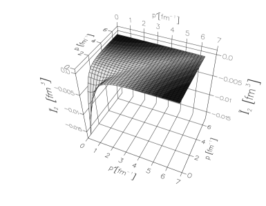
(b)

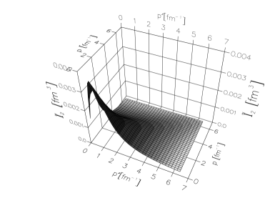
(c)

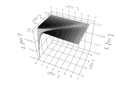
Figure 2: The expression $\tilde{I}_{2}$ from Eq. (LABEL:EQI23), (a) the seagull term, (b) the pionic term and (c) the sum of both. The initial and final states are ¹S₀($\mu$=0) and ³S₁($\mu^{\prime}$ =1), respectively.

(a)

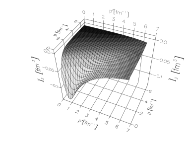
(b)

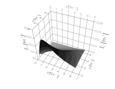
(c)

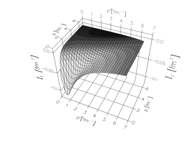
Figure 3: The same as in Fig. 2 for ³P₀($\mu=0$) and ³S₁($\mu^{\prime}=1$).

(a)

(b)

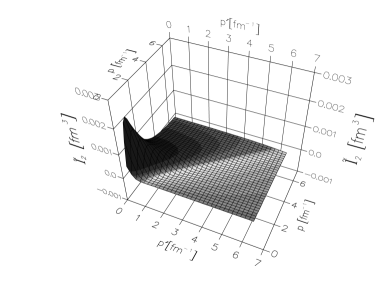
(c)

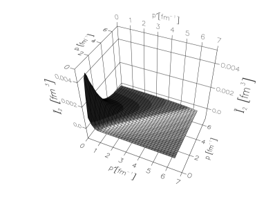
Figure 4: The same as in Fig. 2 for ¹S₀($\mu=0$) and ³D₁($\mu^{\prime}$=1).

(a)

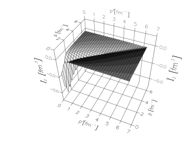
(b)

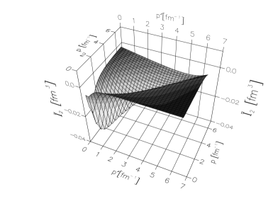
(c)

Figure 5: The same as in Fig. 2 for ³P₀($\mu$=0) and ³S₁($\mu^{\prime}$=1).

Figure 6: The expression $\tilde{I}_{2}$ from (LABEL:EQI23), only the pionic part contributes. The initial and final states are ³P₀($\mu$=0) and ¹P₁($\mu^{\prime}$=1).

5. Summary and Discussion

In this paper we develop three approaches (PWD, 2FI and 4FI) for calculating the matrix elements of the two–nucleon EM currents. We use model [43],[44] of MEC and take into account the contributions originating form $\pi$– and $\rho$–exchanges. The considered MEC satisfy the continuity equation with the one–pion–one–rho–meson exchange potential.

To get the matrix elements of interest we apply the current operator to the 3N bound state and project this vector on 3N basis states $\left|pq\alpha\right>$. The latter are specified by the magnitudes of the Jacobi momenta $p,q$ and the discrete quantum numbers $\alpha$ in $jJ$–coupling. This separation in Eqs.(2.23)–(2.24) of both the operation and the projection can in general work on N-nucleon systems.

The matrix elements in question are contained as building blocks in the amplitudes of the ³He breakup by photons and electrons. We choose this particular form of the matrix elements since it is convenient for incorporation of the corresponding results into the calculations of the reaction amplitudes with full inclusion of the final state interaction.

We express the matrix elements in terms of the multiple integrals. Resorting to the technique of the partial wave decompositions we reduce the matrix elements and arrive at the expressions convenient for the numerical calculations.

For example, the matrix elements of MEC in $\left|pq\alpha\right>$ basis have the form of a superposition of four–dimensional angular integrals. We elaborate two different ways (PWD and 2FI) to diminish the dimensionality of integration and end up with two–fold integrals. One of them, 2FI, is outlined in Section 3. Expressions coming from PWD are given explicitly in Appendices B and C for $\pi$– and $\rho$–MEC, respectively.

Performing the integration over the azimuthal angles in the closed forms (see Section 3), we face tedious analytical calculations. To carry out the second of these integrations one needs to exploit the explicit form of the MEC. This means, in particular, that each model of MEC requires a special treatment within the 2FI procedure.

Aiming to provide a flexibility of the approach, we work out a third procedure (4FI) to compute the discussed four-fold integrals with numerical methods.

We would like to note, that the feasibility of the direct numerical calculation of the reaction amplitudes represented in a form of the multidimensional integrals has been demonstrated in [4]–[8],[42]. The six–dimensional integrals evaluated there have much in common with the ones we deal in this work. In fact, in the both cases an essential element in the integrands is the mixed tensor ${\vec{O}}^{k\kappa}\left(\vec{p}_{2},\vec{p}_{3}\right)$ arising from decomposition of the two–body current. The Korobov method [47] of numerical integration in many dimensions have been applied in Refs.[4]–[8] and [42]. This method proved to be an effective tool for computation of the six-fold integrals.

The detailed analysis show that the results obtained with independent methods (PWD, 2FI and 4FI) are in the perfect agreement. In Section 4 we present benchmark results for the $\pi$–MEC. The momentum dependence of the matrix elements MEC in $\left|pq\alpha\right>$ basis is studied as well.

The potentialities of the approaches elaborated are not restricted by the consideration of the simple two–body currents generated by the $\pi$– and $\rho$–exchange. Other, more complicated, models of the MEC consistent with the realistic NN potentials can be treated without any substantial modifications of the methods.

So, we calculate the matrix elements of the two–body currents in a form providing the compatibility with approach [13]–[17]. The results of the present article are to be used in forthcoming investigations of the quasi–elastic electron scattering off ³He and proton–deuteron radiative capture with inclusion both the MEC and the final state interaction. As it is discussed above, these elements of the theory have to be treated simultaneously for ensuring the gauge independence of the reaction amplitudes and, respectively, for obtaining unambiguous predictions for the observables.

Acknowledgment One of the authors (V. V. K.) would like to thank A.V. Shebeko for the helpful discussions. This work was supported financially (V. V. K.) by the German Ministry for Education, Science and Technology (BMBF No. RUB19960), the Polish Committee for Scientific Research (J. G.) ( grant No. 2P03B03914) and the Deutsche Forschungsgemeinschaft (H. K.). The numerical calculations have been performed on the CRAY T90 and CRAY T3E of the John von Neumann Institute for Computing, Jülich, Germany.

Appendix Appendix A. The partial wave representation of Eq. (2.24)

Eq. (2.24) reads

$$I_{3}(q^{\prime},q,Q;(\lambda^{\prime}{1\over 2})I^{\prime}M^{\prime}-\mu^{\prime},(\lambda{1\over 2})IM-\mu)\equiv\int d\hat{q^{\prime}}{\cal Y}_{I^{\prime},M^{\prime}-\mu^{\prime}}^{*}(\hat{q^{\prime}}){{\delta(q-|\vec{q^{\prime}}+{1\over 3}\vec{Q}|)}\over{q}^{2}}{\cal Y}_{I,M-\mu}(\widehat{\vec{q^{\prime}}+{1\over 3}\vec{Q}}).$$ (A.1)

We use the relations

$${{\delta(q-\left|\vec{q^{\prime}}+{1\over 3}\vec{Q}\right|)}\over{q^{\lambda+2}}}=\sum_{k}2\pi(-)^{k}\sqrt{\hat{k}}h_{k\lambda}(q^{\prime},q,Q){\cal Y}_{kk}^{00}(\hat{q^{\prime}},\hat{Q})$$ (A.2)

with

$$h_{k\lambda}(q^{\prime},q,Q)\equiv\int_{-1}^{1}dxP_{k}(x){{\delta(q-\sqrt{{q^{\prime}}^{2}+Q^{2}/9+2q^{\prime}Qx/3})}\over{q^{\lambda+2}}}$$ (A.3)

and

$$Y_{lm}(\widehat{\vec{a}+\vec{b}})=\sum_{l_{1}+l_{2}=l}{{a^{l_{1}}b^{l_{2}}}\over{|\vec{a}+\vec{b}|^{l}}}\sqrt{{4\pi(2l+1)!}\over{(2l_{1}+1)!(2l_{2}+1)!}}{\cal Y}_{l_{1}l_{2}}^{lm}(\hat{a},\hat{b})$$ (A.4)

Then assuming that the direction of $\vec{Q}$ is parallel to the z- axis we get employing standard steps

$$\begin{array}[]{rl}&I_{3}(q^{\prime},q,Q;(\lambda^{\prime}{1\over 2})I^{\prime}M^{\prime}-\mu^{\prime},(\lambda{1\over 2})IM-\mu)=\delta_{m^{\prime}-\mu^{\prime},m-\mu}{1\over 2}\sqrt{\hat{\lambda}\hat{I}}(-)^{\lambda+I^{\prime}+{1\over 2}}\sqrt{(2\lambda+1)!}\\ &\times\sum_{\lambda_{1}+\lambda_{2}=\lambda}{q^{\prime}}^{\lambda_{1}}({1\over 3}Q)^{\lambda_{2}}{1\over{\sqrt{(2\lambda_{1})!(2\lambda_{2})!}}}\sum_{k}\hat{k}(-)^{k}h_{k}(q^{\prime},q,Q)C(\lambda k\lambda^{\prime},000)\\ &\times\sum_{f}\sqrt{\hat{f}}C(\lambda_{2}kf,000)\left\{\begin{array}[]{ccc}\lambda^{\prime}&f&\lambda\\ \lambda_{2}&\lambda_{1}&k\end{array}\right\}\left\{\begin{array}[]{ccc}f&\lambda&\lambda^{\prime}\\ {1\over 2}&I^{\prime}&I\end{array}\right\}C(f,I,I^{\prime},0,m-\mu).\end{array}$$ (A.12)

Appendix Appendix B. The partial wave representation of Eq. (2.23)

Here we show a spherical component $\zeta$ of $\vec{I}_{2}$ and drop the isospin part. This corresponds to Eq. (LABEL:EQI23). The photon momentum $\hat{Q}$ is assumed to point into the z-direction. We evaluated the seagull part (2.30) and the pionic one (2.31).

$$\tilde{I}_{2}^{seagull}(p^{\prime},p,Q;(l^{\prime}s^{\prime})j^{\prime}\mu^{\prime},(ls)j\mu)$$

$$=-\ 6\sqrt{3}\pi\sqrt{\hat{l}\hat{s}\hat{j}\hat{l^{\prime}}\hat{s^{\prime}}\hat{j^{\prime}}}(-1)^{l^{\prime}+s^{\prime}}\,\delta_{{\mu}^{\prime},{\mu}+\zeta}\$$

$$\times\sum\limits_{\alpha_{1}}(-1)^{\alpha_{1}}\hat{{\alpha_{1}}}\ \left\{{\begin{array}[]{ccc}1&1&{\alpha_{1}}\\ \frac{1}{2}&\frac{1}{2}&s\\ \frac{1}{2}&\frac{1}{2}&s^{\prime}\end{array}}\right\}$$

$$\times\sum\limits_{\alpha_{2}}(-1)^{\alpha_{2}}C(1j\alpha_{2};\zeta\mu{\mu}^{\prime})$$

$$\times\sum\limits_{\alpha_{3}}(-1)^{\alpha_{3}}\hat{{\alpha_{3}}}\ \left\{{\begin{array}[]{ccc}1&{\alpha_{1}}&1\\ l&s&j\\ {\alpha_{3}}&s^{\prime}&{\alpha_{2}}\end{array}}\right\}$$

$$\times\sum\limits_{h_{1}+h_{2}=1}(-1)^{h_{2}}(\frac{1}{2}Q)^{h_{1}}$$

$$\times\sum\limits_{r}\hat{r}[1-(-1)^{\alpha_{1}+h_{2}+r}]$$

$$\times\sum\limits_{f_{1}}\sqrt{\hat{f_{1}}}C(rh_{1}f_{1};000)C(f_{1}j^{\prime}\alpha_{2};0{\mu}^{\prime}{\mu}^{\prime})\left\{{\begin{array}[]{ccc}f_{1}&l^{\prime}&\alpha_{3}\\ s^{\prime}&{\alpha_{2}}&j^{\prime}\end{array}}\right\}$$

$$\times\sum\limits_{f_{2}}\sqrt{\hat{f_{2}}}C(rh_{2}f_{2};000)\sqrt{(2f_{2}+1)!}\left\{{\begin{array}[]{ccc}f_{1}&f_{2}&1\\ l&{\alpha_{3}}&l^{\prime}\end{array}}\right\}\ \left\{{\begin{array}[]{ccc}f_{2}&f_{1}&1\\ h_{1}&h_{2}&r\end{array}}\right\}$$

$$\times\sum\limits_{u_{1}+u_{2}=f_{2}}(p^{\prime})^{\,u_{1}}(p)^{u_{2}}\frac{1}{\sqrt{(2u_{1}+1)!(2u_{2})!}}$$

$$\times\sum\limits_{z}\sqrt{\hat{z}}C(u_{2}lz;000)C(l^{\prime}zu_{1};000)\left\{{\begin{array}[]{ccc}u_{1}&u_{2}&f_{2}\\ l&l^{\prime}&z\end{array}}\right\}\ G^{h_{2}f_{2}}_{zr}{\rm,}$$ (B.1)

where

$$G^{h_{2}f_{2}}_{zr}=\int\limits_{-1}^{1}dyP_{z}(y)\Delta^{h_{2}-f_{2}}\,\int\limits_{-1}^{1}dxP_{r}(x)v_{\pi}(\frac{1}{4}Q^{2}+\Delta^{2}+Q\Delta x)\ \ {\rm and}\ \ \Delta=\sqrt{p^{2}+{p^{\prime}}^{\,2}-2pp^{\prime}y}{\rm.}$$ (B.2)

$$\tilde{I}_{2}^{pionic}(p^{\prime},pQ;(l^{\prime}s^{\prime})j^{\prime}\mu^{\prime},(ls)j\mu)$$

$$=36\pi\sqrt{\hat{l}\hat{s}\hat{j}\hat{l^{\prime}}\hat{s^{\prime}}\hat{j^{\prime}}}(-1)^{l+s^{\prime}}\,\delta_{{\mu}^{\prime},{\mu}+\zeta}\$$

$$\times\sum\limits_{\alpha_{1}}(-1)^{\alpha_{1}}\hat{{\alpha_{1}}}\ \left\{{\begin{array}[]{ccc}1&1&{\alpha_{1}}\\ \frac{1}{2}&\frac{1}{2}&s\\ \frac{1}{2}&\frac{1}{2}&s^{\prime}\end{array}}\right\}$$

$$\times\sum\limits_{e}\hat{e}$$

$$\times\sum\limits_{\alpha_{2}}(-1)^{\alpha_{2}}C(1j\alpha_{2};\zeta\mu{\mu}^{\prime})$$

$$\times\sum\limits_{\alpha_{3}}(-1)^{\alpha_{3}}\hat{{\alpha_{3}}}\ \left\{{\begin{array}[]{ccc}1&{\alpha_{1}}&1\\ l&s&j\\ {\alpha_{3}}&s^{\prime}&{\alpha_{2}}\end{array}}\right\}$$

$$\times\sum\limits_{h_{1}+h_{2}=1}(-1)^{h_{1}}(\frac{1}{2}Q)^{h_{2}}$$

$$\times\sum\limits_{w_{1}+w_{2}=1}(\frac{1}{2}Q)^{w_{2}}$$

$$\times\sum\limits_{d_{1}}\sqrt{\hat{d_{1}}}C(h_{1}w_{1}d_{1};000)$$

$$\times\sum\limits_{d_{2}}\sqrt{\hat{d_{2}}}C(h_{2}w_{2}d_{2};000)\ \left\{{\begin{array}[]{ccc}h_{1}&h_{2}&1\\ w_{1}&w_{2}&1\\ d_{1}&d_{2}&\alpha_{1}\end{array}}\right\}$$

$$\times\sum\limits_{c}\sqrt{\hat{c}}C(d_{1}1c;000)\ \left\{{\begin{array}[]{ccc}d_{2}&d_{1}&\alpha_{1}\\ 1&e&c\end{array}}\right\}$$

$$\times\sum\limits_{f_{1}}\sqrt{\hat{f_{1}}}\left\{{\begin{array}[]{ccc}f_{1}&l^{\prime}&\alpha_{3}\\ s^{\prime}&{\alpha_{2}}&j^{\prime}\end{array}}\right\}(-1)^{f_{1}}\,C(f_{1}j^{\prime}\alpha_{2};0{\mu}^{\prime}{\mu}^{\prime})$$

$$\times\sum\limits_{f_{2}}\sqrt{\hat{f_{2}}}\left\{{\begin{array}[]{ccc}f_{1}&f_{2}&e\\ l&{\alpha_{3}}&l^{\prime}\end{array}}\right\}\ \sqrt{(2f_{2}+1)!}$$

$$\times\sum\limits_{r}\hat{r}C(rd_{2}f_{1};000)C(rcf_{2};000)\left\{{\begin{array}[]{ccc}d_{2}&c&e\\ f_{2}&f_{1}&r\end{array}}\right\}\$$

$$\times\sum\limits_{u_{1}+u_{2}=f_{2}}(p^{\prime})^{\,u_{1}}(p)^{u_{2}}\frac{1}{\sqrt{(2u_{1}+1)!(2u_{2})!}}$$

$$\times\sum\limits_{z}\sqrt{\hat{z}}C(u_{2}lz;000)C(l^{\prime}zu_{1};000)\left\{{\begin{array}[]{ccc}u_{1}&u_{2}&f_{2}\\ l&l^{\prime}&z\end{array}}\right\}\ H^{h_{1}w_{1}f_{2}}_{zr}{\rm,}$$ (B.3)

where

$$H^{h_{1}w_{1}f_{2}}_{zr}=\int\limits_{-1}^{1}dyP_{z}(y)\Delta^{1+h_{1}+w_{1}-f_{2}}\,\int\limits_{-1}^{1}dxP_{r}(x)\frac{v_{\pi}(\frac{1}{4}Q^{2}+\Delta^{2}-Q\Delta x)-v_{\pi}(\frac{1}{4}Q^{2}+\Delta^{2}+Q\Delta x)}{2Q\Delta x}{\rm.}$$ (B.4)

We used the abbreviation $\hat{a}\equiv 2a+1$.

Appendix Appendix C. The $\rho$ Meson Exchange Currents

The $\rho$-meson exchange current are given for instance in [43] and [44]. The current consists of four parts.

$${\vec{j}}_{\rho}({\vec{p}}_{2},{\vec{p}}_{3})\ =\ {\vec{j}}_{\rho,I}({\vec{p}}_{2},{\vec{p}}_{3})\ +{\vec{j}}_{\rho,II}({\vec{p}}_{2},{\vec{p}}_{3})\ +{\vec{j}}_{\rho,III}({\vec{p}}_{2},{\vec{p}}_{3})\ +{\vec{j}}_{\rho,IV}({\vec{p}}_{2},{\vec{p}}_{3})\$$

$${\vec{j}}_{\rho,I}({\vec{p}}_{2},{\vec{p}}_{3})\ \equiv\ i[{\vec{\tau}}(2)\times{\vec{\tau}}(3)]_{z}\ F_{1}^{V}(Q^{2})\ \frac{{\vec{p}}_{2}-{\vec{p}}_{3}}{p_{2}^{2}-p_{3}^{2}}\ \left(v_{\rho}^{s}(p_{3})-v_{\rho}^{s}(p_{2})\right)$$

$${\vec{j}}_{\rho,II}({\vec{p}}_{2},{\vec{p}}_{3})\ \equiv\ -\ i[{\vec{\tau}}(2)\times{\vec{\tau}}(3)]_{z}\ F_{1}^{V}(Q^{2})\$$

$$\times\left(v_{\rho}(p_{3})\,{\vec{\sigma}}(2)\times({\vec{\sigma}}(3)\times{\vec{p}}_{3})\ -\ v_{\rho}(p_{2})\,{\vec{\sigma}}(3)\times({\vec{\sigma}}(2)\times{\vec{p}}_{2})\right)$$

$${\vec{j}}_{\rho,III}({\vec{p}}_{2},{\vec{p}}_{3})\ \equiv\ -\ i[{\vec{\tau}}(2)\times{\vec{\tau}}(3)]_{z}\ F_{1}^{V}(Q^{2})\ \frac{v_{\rho}(p_{3})-v_{\rho}(p_{2})}{p_{2}^{2}-p_{3}^{2}}\ \left(({\vec{\sigma}}(2)\times{\vec{p}}_{2})\cdot({\vec{\sigma}}(3)\times{\vec{p}}_{3})\right)({\vec{p}}_{2}-{\vec{p}}_{3})$$

$${\vec{j}}_{\rho,IV}({\vec{p}}_{2},{\vec{p}}_{3})\ \equiv\ -\ i[{\vec{\tau}}(2)\times{\vec{\tau}}(3)]_{z}\ F_{1}^{V}(Q^{2})\ \frac{v_{\rho}(p_{3})-v_{\rho}(p_{2})}{p_{2}^{2}-p_{3}^{2}}\$$

$$\times\left({\vec{\sigma}}(3)\cdot({\vec{p}}_{2}\times{\vec{p}}_{3})({\vec{\sigma}}(2)\times{\vec{p}}_{2})\ +\ {\vec{\sigma}}(2)\cdot({\vec{p}}_{2}\times{\vec{p}}_{3})({\vec{\sigma}}(3)\times{\vec{p}}_{3})\right){\rm.}$$

First we present their PWD for the spherical component $\zeta$ :

$$\tilde{I}_{2}^{I\rho}(p^{\prime},p,Q;(l^{\prime}s^{\prime})j^{\prime}\mu^{\prime},(ls)j\mu)$$

$$=2\pi\sqrt{\hat{l}\hat{j}\hat{l^{\prime}}}(-1)^{l+j^{\prime}}\,\delta_{s^{\prime},s}\ \delta_{{\mu}^{\prime},{\mu}+\zeta}\$$

$$\times\sum\limits_{\alpha_{2}}\sqrt{\hat{{\alpha_{2}}}}(-1)^{\alpha_{2}}C(1j\alpha_{2};\zeta\mu{\mu}^{\prime})$$

$$\times\sum\limits_{\alpha_{3}}(-1)^{\alpha_{3}}\hat{{\alpha_{3}}}\ \left\{{\begin{array}[]{ccc}1&l&{\alpha_{3}}\\ s&{\alpha_{2}}&j\end{array}}\right\}$$

$$\times\sum\limits_{r}\hat{r}\left\{{\begin{array}[]{ccc}r&{\alpha_{3}}&l^{\prime}\\ s^{\prime}&j^{\prime}&{\alpha_{2}}\end{array}}\right\}\ C(r{\alpha_{2}}j^{\prime};0{\mu}^{\prime}{\mu}^{\prime})$$

$$\times\sum\limits_{\alpha_{4}}\sqrt{\hat{\alpha_{4}}}\,(-1)^{\alpha_{4}}\,\sqrt{(2\alpha_{4}+1)!}C(r1\alpha_{4};000)\,\left\{{\begin{array}[]{ccc}r&1&{\alpha_{4}}\\ l&l^{\prime}&{\alpha_{3}}\end{array}}\right\}\$$

$$\times\sum\limits_{u_{1}+u_{2}=\alpha_{4}}(p^{\prime})^{\,u_{1}}(p)^{u_{2}}(-1)^{u_{2}}\frac{1}{\sqrt{(2u_{1}+1)!(2u_{2})!}}$$

$$\times\sum\limits_{z}\sqrt{\hat{z}}(-1)^{z}C(u_{2}lz;000)C(l^{\prime}zu_{1};000)\left\{{\begin{array}[]{ccc}u_{1}&u_{2}&\alpha_{4}\\ l&l^{\prime}&z\end{array}}\right\}\ H^{\alpha_{4}}_{zr}{\rm,}$$ (C.1)

where

$$H^{\alpha_{4}}_{zr}=\int\limits_{-1}^{1}dyP_{z}(y)\Delta^{1-\alpha_{4}}\,\int\limits_{-1}^{1}dxP_{r}(x)\frac{v_{\rho}^{s}(\frac{1}{4}Q^{2}+\Delta^{2}-Q\Delta x)-v_{\rho}^{s}(\frac{1}{4}Q^{2}+\Delta^{2}+Q\Delta x)}{2Q\Delta x}{\rm.}$$ (C.2)

$$\tilde{I}_{2}^{II\rho}(p^{\prime},p,Q;(l^{\prime}s^{\prime})j^{\prime}\mu^{\prime},(ls)j\mu)$$

$$=36\pi\sqrt{3}\,\sqrt{\hat{l}\hat{s}\hat{j}\hat{l^{\prime}}\hat{s^{\prime}}\hat{j^{\prime}}}(-1)^{s^{\prime}}\,\delta_{{\mu}^{\prime},{\mu}+\zeta}\$$

$$\times\sum\limits_{\alpha_{1}}(-1)^{\alpha_{1}}\hat{{\alpha_{1}}}\ \left\{{\begin{array}[]{ccc}1&1&{\alpha_{1}}\\ 1&1&1\end{array}}\right\}\ \left\{{\begin{array}[]{ccc}1&1&{\alpha_{1}}\\ \frac{1}{2}&\frac{1}{2}&s\\ \frac{1}{2}&\frac{1}{2}&s^{\prime}\end{array}}\right\}$$

$$\times\sum\limits_{u_{1}+u_{2}=1}(-1)^{u_{1}}(\frac{1}{2}Q)^{u_{2}}$$

$$\times\sum\limits_{r}(-1)^{r}\hat{r}\,[1-(-1)^{\alpha_{1}+u_{1}+r}]$$

$$\times\sum\limits_{f_{1}}\sqrt{\hat{f_{1}}}(-1)^{f_{1}}\,\sqrt{(2f_{1}+1)!}\,C(ru_{1}f_{1};000)$$

$$\times\sum\limits_{f_{2}}\sqrt{\hat{f_{2}}}(-1)^{f_{2}}\,\left\{{\begin{array}[]{ccc}f_{2}&f_{1}&1\\ u_{1}&u_{2}&r\end{array}}\right\}\ C(ru_{2}f_{2};000)$$

$$\times\sum\limits_{\alpha_{2}}(-1)^{\alpha_{2}}C(1j\alpha_{2};\zeta\mu{\mu}^{\prime})\,C(f_{2}j^{\prime}\alpha_{2};0{\mu}^{\prime}{\mu}^{\prime})$$

$$\times\sum\limits_{\alpha_{3}}(-1)^{\alpha_{3}}\hat{{\alpha_{3}}}\ \left\{{\begin{array}[]{ccc}1&{\alpha_{1}}&1\\ l&s&j\\ {\alpha_{3}}&s^{\prime}&{\alpha_{2}}\end{array}}\right\}\ \left\{{\begin{array}[]{ccc}f_{2}&f_{1}&1\\ l&\alpha_{3}&l^{\prime}\end{array}}\right\}\left\{{\begin{array}[]{ccc}f_{2}&l^{\prime}&\alpha_{3}\\ s^{\prime}&\alpha_{2}&j^{\prime}\end{array}}\right\}$$

$$\times\sum\limits_{w_{1}+w_{2}=f_{1}}(p^{\prime})^{\,w_{1}}(p)^{w_{2}}(-1)^{w_{2}}\frac{1}{\sqrt{(2w_{1}+1)!(2w_{2})!}}$$

$$\times\sum\limits_{z}\sqrt{\hat{z}}(-1)^{z}\,C(w_{2}lz;000)C(l^{\prime}zw_{1};000)\left\{{\begin{array}[]{ccc}w_{1}&w_{2}&f_{1}\\ l&l^{\prime}&z\end{array}}\right\}\ H^{u_{1}f_{1}}_{zr}{\rm,}$$ (C.3)

where

$$H^{u_{1}f_{1}}_{zr}=-\int\limits_{-1}^{1}dyP_{z}(y)\Delta^{u_{1}-f_{1}}\,\int\limits_{-1}^{1}dxP_{r}(x)v_{\rho}(\frac{1}{4}Q^{2}+\Delta^{2}-Q\Delta x){\rm.}$$ (C.4)

$$\tilde{I}_{2}^{III\rho}(p^{\prime},p,Q;(l^{\prime}s^{\prime})j^{\prime}\mu^{\prime},(ls)j\mu)$$

$$=-216\pi\sqrt{\hat{l}\hat{s}\hat{j}\hat{l^{\prime}}\hat{s^{\prime}}\hat{j^{\prime}}}(-1)^{l+s^{\prime}}\,\delta_{{\mu}^{\prime},{\mu}+\zeta}\ =$$

$$\times\sum\limits_{\alpha_{1}}\hat{{\alpha_{1}}}\ \left\{{\begin{array}[]{ccc}1&1&1\\ 1&1&{\alpha_{1}}\end{array}}\right\}\ \left\{{\begin{array}[]{ccc}1&1&{\alpha_{1}}\\ \frac{1}{2}&\frac{1}{2}&s\\ \frac{1}{2}&\frac{1}{2}&s^{\prime}\end{array}}\right\}$$

$$\times\sum\limits_{e}\hat{e}$$

$$\times\sum\limits_{\alpha_{2}}(-1)^{\alpha_{2}}C(1j\alpha_{2};\zeta\mu{\mu}^{\prime})$$

$$\times\sum\limits_{\alpha_{3}}(-1)^{\alpha_{3}}\hat{{\alpha_{3}}}\ \left\{{\begin{array}[]{ccc}1&{\alpha_{1}}&1\\ l&s&j\\ {\alpha_{3}}&s^{\prime}&{\alpha_{2}}\end{array}}\right\}$$

$$\times\sum\limits_{h_{1}+h_{2}=1}(-1)^{h_{1}}(\frac{1}{2}Q)^{h_{2}}$$

$$\times\sum\limits_{w_{1}+w_{2}=1}(\frac{1}{2}Q)^{w_{2}}$$

$$\times\sum\limits_{d_{1}}\sqrt{\hat{d_{1}}}C(h_{1}w_{1}d_{1};000)$$

$$\times\sum\limits_{d_{2}}\sqrt{\hat{d_{2}}}C(h_{2}w_{2}d_{2};000)\ \left\{{\begin{array}[]{ccc}h_{1}&h_{2}&1\\ w_{1}&w_{2}&1\\ d_{1}&d_{2}&\alpha_{1}\end{array}}\right\}$$

$$\times\sum\limits_{c}\sqrt{\hat{c}}C(d_{1}1c;000)\ \left\{{\begin{array}[]{ccc}d_{2}&d_{1}&\alpha_{1}\\ 1&e&c\end{array}}\right\}$$

$$\times\sum\limits_{f_{1}}\sqrt{\hat{f_{1}}}\left\{{\begin{array}[]{ccc}f_{1}&l^{\prime}&\alpha_{3}\\ s^{\prime}&{\alpha_{2}}&j^{\prime}\end{array}}\right\}(-1)^{f_{1}}\,C(f_{1}j^{\prime}\alpha_{2};0{\mu}^{\prime}{\mu}^{\prime})$$

$$\times\sum\limits_{f_{2}}\sqrt{\hat{f_{2}}}\left\{{\begin{array}[]{ccc}f_{1}&f_{2}&e\\ l&{\alpha_{3}}&l^{\prime}\end{array}}\right\}\ \sqrt{(2f_{2}+1)!}$$

$$\times\sum\limits_{r}\hat{r}C(rd_{2}f_{1};000)C(rcf_{2};000)\left\{{\begin{array}[]{ccc}d_{2}&c&e\\ f_{2}&f_{1}&r\end{array}}\right\}\$$

$$\times\sum\limits_{u_{1}+u_{2}=f_{2}}(p^{\prime})^{\,u_{1}}(p)^{u_{2}}\frac{1}{\sqrt{(2u_{1}+1)!(2u_{2})!}}$$

$$\times\sum\limits_{z}\sqrt{\hat{z}}C(u_{2}lz;000)C(l^{\prime}zu_{1};000)\left\{{\begin{array}[]{ccc}u_{1}&u_{2}&f_{2}\\ l&l^{\prime}&z\end{array}}\right\}\ H^{h_{1}w_{1}f_{2}}_{zr}{\rm,}$$ (C.5)

where

$$H^{h_{1}w_{1}f_{2}}_{zr}=-\int\limits_{-1}^{1}dyP_{z}(y)\Delta^{1+h_{1}+w_{1}-f_{2}}\,\int\limits_{-1}^{1}dxP_{r}(x)\frac{v_{\rho}(\frac{1}{4}Q^{2}+\Delta^{2}-Q\Delta x)-v_{\rho}(\frac{1}{4}Q^{2}+\Delta^{2}+Q\Delta x)}{2Q\Delta x}{\rm.}$$ (C.6)

$$\tilde{I}_{2}^{IV\rho}(p^{\prime},p,Q;(l^{\prime}s^{\prime})j^{\prime}\mu^{\prime},(ls)j\mu)$$

$$=-36\pi\sqrt{3}\sqrt{\hat{l}\hat{s}\hat{j}\hat{l^{\prime}}\hat{s^{\prime}}\hat{j^{\prime}}}(-1)^{l+s+j}\,\delta_{{\mu}^{\prime},{\mu}+\zeta}\$$

$$\times\sum\limits_{\alpha_{1}}\hat{{\alpha_{1}}}\ \left\{{\begin{array}[]{ccc}1&1&{\alpha_{1}}\\ \frac{1}{2}&\frac{1}{2}&s\\ \frac{1}{2}&\frac{1}{2}&s^{\prime}\end{array}}\right\}$$

$$\times\sum\limits_{\alpha_{2}}\hat{{\alpha_{2}}}\ \left\{{\begin{array}[]{ccc}1&1&1\\ \alpha_{2}&\alpha_{1}&1\end{array}}\right\}$$

$$\times\sum\limits_{u_{1}+u_{2}=1}(\frac{1}{2}Q)^{u_{2}}$$

$$\times\sum\limits_{\alpha_{3}}\,C(1j{\alpha_{3}};\zeta\mu{\mu}^{\prime})$$

$$\times\sum\limits_{h}\hat{h}\ \left\{{\begin{array}[]{ccc}\alpha_{1}&\alpha_{2}&1\\ s&l&j\\ s^{\prime}&h&\alpha_{3}\end{array}}\right\}$$

$$\times\sum\limits_{f_{1}}\sqrt{\hat{f_{1}}}C(1u_{1}f_{1};000)$$

$$\times\sum\limits_{f_{2}}\sqrt{\hat{f_{2}}}C(1u_{2}f_{2};000)\left\{{\begin{array}[]{ccc}1&1&1\\ u_{1}&u_{2}&1\\ f_{1}&f_{2}&\alpha_{1}\end{array}}\right\}$$

$$\times\sum\limits_{g_{1}}\sqrt{\hat{g_{1}}}\sqrt{(2g_{1}+1)!}$$

$$\times\sum\limits_{g_{2}}\sqrt{\hat{g_{2}}}\left\{{\begin{array}[]{ccc}g_{2}&l^{\prime}&h\\ s^{\prime}&\alpha_{3}&j^{\prime}\end{array}}\right\}\ \left\{{\begin{array}[]{ccc}g_{2}&g_{1}&\alpha_{2}\\ l&h&l^{\prime}\end{array}}\right\}$$

$$\times\sum\limits_{r}\hat{r}(-1)^{r}\ C(rf_{1}g_{1};000)C(rf_{2}g_{2};000)\left\{{\begin{array}[]{ccc}g_{2}&g_{1}&\alpha_{2}\\ f_{1}&f_{2}&r\end{array}}\right\}\ [1+(-1)^{\alpha_{1}+u_{1}+r}]$$

$$\times\sum\limits_{w_{1}+w_{2}=g_{1}}(p^{\prime})^{\,w_{1}}(p)^{w_{2}}(-1)^{w_{2}}\frac{1}{\sqrt{(2w_{1}+1)!(2w_{2})!}}$$

$$\times\sum\limits_{z}\sqrt{\hat{z}}(-1)^{z}C(w_{2}lz;000)C(l^{\prime}zw_{1};000)\left\{{\begin{array}[]{ccc}w_{1}&w_{2}&g_{1}\\ l&l^{\prime}&z\end{array}}\right\}\ H^{u_{1}g_{1}}_{zr}{\rm,}$$ (C.7)

where

$$H^{u_{1}g_{1}}_{zr}=-\int\limits_{-1}^{1}dyP_{z}(y)\Delta^{1+u_{1}-g_{1}}\,\int\limits_{-1}^{1}dxP_{r}(x)\frac{v_{\rho}(\frac{1}{4}Q^{2}+\Delta^{2}-Q\Delta x)-v_{\rho}(\frac{1}{4}Q^{2}+\Delta^{2}+Q\Delta x)}{2Q\Delta x}{\rm.}$$ (C.8)

Secondly we present the form required for the 4-fold integration. The separation of spin and momentum parts like in (2.33), is also displayed for the convenience of the reader. The first term $j^{I,\rho}$ has no spin-dependence and is left at it is.

$$\tilde{I}_{2}^{II\rho}(p^{\prime},p,Q;(l^{\prime}s^{\prime})j^{\prime}\mu^{\prime},(ls)j\mu)$$ (C.9)

$$=\sum_{m,m^{\prime}}C(lsj,\mu-m,m)C(l^{\prime}s^{\prime}j^{\prime},\mu^{\prime}-m^{\prime},m^{\prime})\int d\hat{p}d\hat{p^{\prime}}Y^{*}_{l^{\prime}\mu^{\prime}-m^{\prime}}(\hat{p^{\prime}})Y_{l\mu-m}(\hat{p})$$

$$\times 6\sum_{\alpha_{1}\nu}\left\{{\begin{array}[]{ccc}1&1&\alpha_{1}\\ 1&1&1\end{array}}\right\}C(\alpha_{1}11,\nu-\zeta,\zeta,\nu)\left\{\sigma(2)\otimes\sigma(3)\right\}_{\alpha_{1}\nu}$$

$$\times[-v_{\rho}(p_{3})(-)^{-\nu+\zeta}(p_{3})_{\zeta-\nu}+v_{\rho}(p_{2})(-)^{\alpha_{1}-\nu+\zeta}(p_{2})_{\zeta-\nu}]{\rm,}$$

$$\tilde{I}_{2}^{III\rho}(p^{\prime},p,Q;(l^{\prime}s^{\prime})j^{\prime}\mu^{\prime},(ls)j\mu)$$ (C.10)

$$=\sum_{m,m^{\prime}}C(lsj,\mu-m,m)C(l^{\prime}s^{\prime}j^{\prime},\mu^{\prime}-m^{\prime},m^{\prime})\int d\hat{p}d\hat{p^{\prime}}Y^{*}_{l^{\prime}\mu^{\prime}-m^{\prime}}(\hat{p^{\prime}})Y_{l\mu-m}(\hat{p})$$

$$\times\frac{({\vec{p}}_{2}-{\vec{p}}_{3})_{\zeta}}{p_{2}^{2}-p_{3}^{2}}\ \left(v_{\rho}(p_{2})-v_{\rho}(p_{3})\right)$$

$$\times 6\sum_{\alpha_{1}\nu}(-)^{1-\nu}\left\{{\begin{array}[]{ccc}1&1&1\\ 1&1&\alpha_{1}\end{array}}\right\}\left\{\sigma(2)\otimes\sigma(3)\right\}_{\alpha_{1}\nu}\left\{p_{2}\otimes p_{3}\right\}_{\alpha_{1},-\nu}{\rm,}$$

$$\tilde{I}_{2}^{IV\rho}(p^{\prime},p,Q;(l^{\prime}s^{\prime})j^{\prime}\mu^{\prime},(ls)j\mu)$$ (C.11)

$$=\sum_{m,m^{\prime}}C(lsj,\mu-m,m)C(l^{\prime}s^{\prime}j^{\prime},\mu^{\prime}-m^{\prime},m^{\prime})\int d\hat{p}d\hat{p^{\prime}}Y^{*}_{l^{\prime}\mu^{\prime}-m^{\prime}}(\hat{p^{\prime}})Y_{l\mu-m}(\hat{p})$$

$$\times\frac{v_{\rho}(p_{2})-v_{\rho}(p_{3})}{p_{2}^{2}-p_{3}^{2}}\ \sum_{\alpha_{1}\alpha_{2}}(-2)\sqrt{\hat{\alpha}_{1}\hat{\alpha}_{2}}\left\{{\begin{array}[]{ccc}1&1&1\\ \alpha_{1}&\alpha_{2}&1\end{array}}\right\}(-1)^{\alpha_{2}}$$

$$\times\sum_{\kappa}C(\alpha_{1}\alpha_{2}1,\kappa,\zeta-\kappa,\zeta)\left\{\sigma(2)\otimes\sigma(3)\right\}_{\alpha_{1}\kappa}\sum_{\kappa_{2}\kappa_{3}}C(11\alpha_{2},-\kappa_{2}-\kappa_{3}+\zeta-\kappa,\kappa_{2}+\kappa_{3},\zeta-\kappa)$$

$$\times C(111,\kappa_{2},\kappa_{3},\kappa_{2}+\kappa_{3})\left\{(p_{2})_{\kappa_{4}}(p_{2})_{\kappa_{2}}(p_{3})_{\kappa_{3}}+(-)^{1+\alpha_{1}}(p_{3})_{\kappa_{4}}(p_{3})_{\kappa_{2}}(p_{2})_{\kappa_{3}}\right\}{\rm,}$$

with $\kappa_{4}=-\kappa_{2}-\kappa_{3}+\zeta-\kappa$. The momenta $p_{2}$ and $p_{3}$ are given in Eqs. (2.19).

Appendix Appendix D. Functions $F$ and $G$ in the Case of $\pi$–Meson Exchange Currents

We have for the seagull contributions (3.6)–(3.)

$$\begin{array}[]{lll}\lx@intercol\@ADDCLASS{ltx_eqn_lefteqn}$\displaystyle G^{l^{\prime}m^{\prime}}_{lm}(n)=\delta_{m^{\prime},m}$\mbox{}\hfil\lx@intercol&&\\ &\times&{\displaystyle{1\over\pi}}{\displaystyle\int\limits_{-1}^{+1}dx\int\limits_{-1}^{+1}dx^{\prime}}\>\bar{P}^{m^{\prime}}_{l^{\prime}}(x^{\prime})\bar{P}^{m}_{l}(x)V(m,n),\end{array}$$ (D.1)

$$\begin{array}[]{lll}\lx@intercol\@ADDCLASS{ltx_eqn_lefteqn}$\displaystyle G^{l^{\prime}m^{\prime}}_{lm\mu}(n)=\delta_{m^{\prime},m+\mu}$\mbox{}\hfil\lx@intercol&&\\ &\times&{\displaystyle{1\over\pi}}{\displaystyle\left({2\over 3}\right)^{1/2}}{\displaystyle\int\limits_{-1}^{+1}dx\int\limits_{-1}^{+1}dx^{\prime}}\>\bar{P}^{m^{\prime}}_{l^{\prime}}(x^{\prime})\bar{P}^{m}_{l}(x)\\ &\times&\left(p^{\prime}\bar{P}^{\mu}_{1}(x^{\prime})V(m,n)-p\bar{P}^{\mu}_{1}(x)V(m+\mu,n)\right)\end{array}$$ (D.2)

and for the ones (3.8)–(3.10) of the pionic current

$$\begin{array}[]{lll}\lx@intercol\@ADDCLASS{ltx_eqn_lefteqn}$\displaystyle F^{l^{\prime}m^{\prime}}_{lm\mu}=\delta_{m^{\prime},m+\mu}$\mbox{}\hfil\lx@intercol&&\\ &\times&{\displaystyle{1\over\pi}}{\displaystyle\left({2\over 3}\right)^{1/2}}{\displaystyle\int\limits_{-1}^{+1}dx\int\limits_{-1}^{+1}dx^{\prime}}\>\bar{P}^{m^{\prime}}_{l^{\prime}}(x^{\prime})\bar{P}^{m}_{l}(x)\\ &\times&\left(p^{\prime}\bar{P}^{\mu}_{1}(x^{\prime})W(m)-p\bar{P}^{\mu}_{1}(x)W(m+\mu)\right),\end{array}$$ (D.3)

$$\begin{array}[]{lll}\lx@intercol\@ADDCLASS{ltx_eqn_lefteqn}$\displaystyle F^{l^{\prime}m^{\prime}}_{lm\mu_{1}\mu_{2}}=\delta_{m^{\prime},m+\mu_{1}+\mu_{2}}$\mbox{}\hfil\lx@intercol&&\\ &\times&{\displaystyle{2\over 3\pi}}{\displaystyle\int\limits_{-1}^{+1}dx\int\limits_{-1}^{+1}dx^{\prime}}\>\bar{P}^{m^{\prime}}_{l^{\prime}}(x^{\prime})\bar{P}^{m}_{l}(x)\\ &\times&\left(p^{\prime 2}\bar{P}^{\mu_{1}}_{1}(x^{\prime})\bar{P}^{\mu_{2}}_{1}(x^{\prime})W(m)\right.\\ &-&pp^{\prime}\bar{P}^{\mu_{1}}_{1}(x^{\prime})\bar{P}^{\mu_{2}}_{1}(x)W(m+\mu_{2})\\ &-&pp^{\prime}\bar{P}^{\mu_{1}}_{1}(x)\bar{P}^{\mu_{2}}_{1}(x^{\prime})W(m+\mu_{1})\\ &+&\left.p^{2}\bar{P}^{\mu_{1}}_{1}(x^{\prime})\bar{P}^{\mu_{2}}_{1}(x)W(m+\mu_{1}+\mu_{2})\right),\end{array}$$ (D.4)

$$\begin{array}[]{lll}\lx@intercol\@ADDCLASS{ltx_eqn_lefteqn}$\displaystyle F^{l^{\prime}m^{\prime}}_{lm\mu_{1}\mu_{2}\mu_{3}}=\delta_{m^{\prime},m+\mu_{1}+\mu_{2}+\mu_{3}}$\mbox{}\hfil\lx@intercol&&\\ &\times&{\displaystyle{1\over\pi}}{\displaystyle\left({2\over 3}\right)^{1/2}}{\displaystyle\int\limits_{-1}^{+1}dx\int\limits_{-1}^{+1}dx^{\prime}}\>\bar{P}^{m^{\prime}}_{l^{\prime}}(x^{\prime})\bar{P}^{m}_{l}(x)\\ &\times&\left(p^{\prime 3}\bar{P}^{\mu_{1}}_{1}(x^{\prime})\bar{P}^{\mu_{2}}_{1}(x^{\prime})\bar{P}^{\mu_{3}}_{1}(x^{\prime})W(m)\right.\\ &-&p^{\prime 2}p\bar{P}^{\mu_{1}}_{1}(x)\bar{P}^{\mu_{2}}_{1}(x^{\prime})\bar{P}^{\mu_{3}}_{1}(x^{\prime})W(m+\mu_{1})\\ &-&p^{\prime 2}p\bar{P}^{\mu_{1}}_{1}(x^{\prime})\bar{P}^{\mu_{2}}_{1}(x)\bar{P}^{\mu_{3}}_{1}(x^{\prime})W(m+\mu_{2})\\ &+&p^{\prime}p^{2}\bar{P}^{\mu_{1}}_{1}(x)\bar{P}^{\mu_{2}}_{1}(x)\bar{P}^{\mu_{3}}_{1}(x^{\prime})W(m+\mu_{1}+\mu_{2})\\ &-&p^{\prime 2}p\bar{P}^{\mu_{1}}_{1}(x^{\prime})\bar{P}^{\mu_{2}}_{1}(x^{\prime})\bar{P}^{\mu_{3}}_{1}(x)W(m+\mu_{3})\\ &+&p^{\prime}p^{2}\bar{P}^{\mu_{1}}_{1}(x)\bar{P}^{\mu_{2}}_{1}(x^{\prime})\bar{P}^{\mu_{3}}_{1}(x)W(m+\mu_{1}+\mu_{3})\\ &+&p^{\prime}p^{2}\bar{P}^{\mu_{1}}_{1}(x^{\prime})\bar{P}^{\mu_{2}}_{1}(x)\bar{P}^{\mu_{3}}_{1}(x)W(m+\mu_{2}+\mu_{3})\\ &-&\left.p^{\prime 3}\bar{P}^{\mu_{1}}_{1}(x)\bar{P}^{\mu_{2}}_{1}(x)\bar{P}^{\mu_{3}}_{1}(x)W(m+\mu_{1}+\mu_{2}+\mu_{3})\right)\end{array}$$ (D.5)

with

$$\bar{P}^{m}_{l}(cos\theta)\equiv\sqrt{2\pi}~{}~{}e^{-im\phi}~{}~{}Y_{lm}(\theta,\phi).$$ (D.6)

Note, that formulae (D.1)–(D.5) have been obtained in the coordinate system where $\vec{Q}\parallel{\vec{e}}_{z}$.

Appendix Appendix E. Integrals over the Azimuthal Angle

The integrands of (3.6)–(3.10) contain functions

$$v(p)={\displaystyle\frac{f^{2}_{\pi NN}}{2\pi^{2}m^{2}_{\pi}}}F_{\pi NN}(m^{2}_{\pi}+p^{2})^{-1}\qquad\mbox{and}\qquad H(p_{2},p_{3})=(p_{3}^{2}-p_{2}^{2})^{-1}(v(p_{2})-v(p_{3})).$$

In Appendix D we list the expressions for $F$ and $G$ (Eqs.(3.6)–(3.10)) in terms of two–dimensional integrals over the products of the associated Legendre polynomials ${\bar{P}}^{m}_{l}(x)$ and the integrals

$$\begin{array}[]{rcl}V(m,n)={\displaystyle\int\limits_{0}^{2\pi}}dt(2t-t)\cos(mt)v(p_{n}),&\mbox{and}&W(m)={\displaystyle\int\limits_{0}^{2\pi}}dt(2t-t)\cos(mt)H(p_{2},p_{3}).\end{array}$$ (E.1)

Functions (E.1) belong to the type of integral (3.14). To compute (E.1) analytically with $v(p_{n})$ and $H(p_{2},p_{3})$ in question we write for the vector $\vec{p}_{n}$ (3.2)

$$p_{n}^{2}=a_{n}+b\cos t$$ (E.2)

where

$$a_{n} = {\displaystyle 1\over 4}Q^{2}+p^{\prime 2}+p^{2}+(-1)^{n}\vec{Q}(\vec{p}\;^{\prime}-\vec{p})-2p^{\prime}p\>\cos\theta\>\cos\theta^{\prime},$$ (E.3)

$$b = -2p^{\prime}p\>\sin\theta\>\sin\theta^{\prime}$$ (E.4)

and decompose

$$v(p_{n}) = {\displaystyle\frac{f^{2}_{\pi NN}}{2\pi^{2}m^{2}_{\pi}}}\left[(a_{n}+m^{2}_{\pi}+b\cos t)^{-1}-(a_{n}+\Lambda^{2}_{\pi}+b\cos t)^{-1}\right.$$ (E.5)

$$\phantom{{\displaystyle\frac{f^{2}_{\pi NN}}{2\pi^{2}m^{2}_{\pi}}}}\left.-(\Lambda^{2}_{\pi}-m^{2}_{\pi})(a_{n}+\Lambda^{2}_{\pi}+b\cos t)^{-2}\right],$$

$$H(p_{2},p_{3}) = {\displaystyle\frac{f^{2}_{\pi NN}}{2\pi^{2}m^{2}_{\pi}}}(a_{2}-a_{3})^{-1}$$ (E.6)

$$\left[-(a_{2}+m^{2}_{\pi}+b\cos t)^{-1}+(a_{3}+m^{2}_{\pi}+b\cos t)^{-1}\right.$$

$$+(a_{2}+\Lambda^{2}_{\pi}+b\cos t)^{-1}-(a_{3}+\Lambda^{2}_{\pi}+b\cos t)^{-1}$$

$$\left.+(\Lambda^{2}_{\pi}-m^{2}_{\pi})((a_{2}+\Lambda^{2}_{\pi}+b\cos t)^{-2}-(a_{3}+\Lambda^{2}_{\pi}+b\cos t)^{-2}\right].$$

We get

$$V(m,n) = {\displaystyle\frac{f^{2}_{\pi NN}}{2\pi^{2}m^{2}_{\pi}}}\left[V(a_{n}+m^{2}_{\pi},\>b,\>m,\>1)-V(a_{n}+\Lambda^{2}_{\pi},\>b,\>m,\>1)\right.$$ (E.7)

$$\phantom{{\displaystyle\frac{f^{2}_{\pi NN}}{2\pi^{2}m^{2}_{\pi}}}}\left.-(\Lambda^{2}_{\pi}-m^{2}_{\pi})V(a_{n}+\Lambda^{2}_{\pi},\>b,\>m,\>2)\right],$$

$$W(m) = {\displaystyle\frac{f^{2}_{\pi NN}}{2\pi^{2}m^{2}_{\pi}}}(a_{2}-a_{3})^{-1}$$ (E.8)

$$\phantom{{\displaystyle\frac{f^{2}_{\pi NN}}{2\pi^{2}m^{2}_{\pi}}}}\left[-V(a_{2}+m^{2}_{\pi},\>b,\>m,\>1)+V(a_{3}+m^{2}_{\pi},\>b,\>m,\>1)\right.$$

$$\phantom{{\displaystyle\frac{f^{2}_{\pi NN}}{2\pi^{2}m^{2}_{\pi}}}}+V(a_{2}+\Lambda^{2}_{\pi},\>b,\>m,\>1)-V(a_{3}+\Lambda^{2}_{\pi},\>b,\>m,\>1)$$

$$\phantom{{\displaystyle\frac{f^{2}_{\pi NN}}{2\pi^{2}m^{2}_{\pi}}}}\left.+(\Lambda^{2}_{\pi}-m^{2}_{\pi})(V(a_{2}+\Lambda^{2}_{\pi},\>b,\>m,\>2)-V(a_{3}+\Lambda^{2}_{\pi},\>b,\>m,\>2))\right].$$

Integrals (3.17) can be calculated in closed form, e.g., with the help of tables [48]. For $m\geq 0$ and $n=1,2$ the result reads

$$V(a,b,m,n) = 2\pi^{2}\left[{\displaystyle 1\over b}\left(\sqrt{a^{2}-b^{2}}-a\right)\right]^{m}$$ (E.9)

$$\times (a^{2}-b^{2})^{-n+\scriptstyle{\frac{1}{2}}}\>\left(a+m\sqrt{a^{2}-b^{2}}\right)^{n-1},$$

for $m,0$ one can use the relation $V(m,n)=V(-m,n).$

References

• [1]
• [2] E. van Meijgaard and J. A. Tjon, Phys. Rev. C42 (1990) 74; C42 (1990) 96; C45 (1992) 1463.
• [3] J. L. Friar, B. F. Gibson and G. L. Payne, Phys.Lett. B251 (1990) 11.
• [4] V. V. Kotlyar and A. V. Shebeko, Sov. J. Nucl. Phys. 51 (1990) 645; 52 (1990) 836; 54 (1991) 423.
• [5] V. V. Kotlyar, Proc. of the Nat. Conf. on Phys. of Few–Body and Quark–Hadronic Syst., eds. V. Boldyshev et al., Kharkov, 1992, (Kharkov, 1994), p. 145.
• [6] V. V. Kotlyar, Yu. P. Mel’nik and A. V. Shebeko, Phys. Part. and Nucl. 26 (1995) 79.
• [7] V. V. Kotlyar, Proc. of the 3rd Int. Symposium ”Dubna Deuteron-95” (July 1995, Dubna). Dubna, 1996, p. 221.
• [8] V. V. Kotlyar Proc. of the 12th Int. Symposium on High-Energy Spin Phys. (September, 1996, Amsterdam). Eds. C.W. de Jager, T.J.Ketel, P.J.Mulders, J.E.J.Oberski and M.Oskam-Tamboezer World Scientific, 1997, p. 402.
• [9] A. C. Fonseca and D. R. Lehman, Phys.Lett. B267 (1991) 159; Phys. Rev. C48 (1993) R503.
• [10] G. J. Schmid, R. M. Chasteler, H. R. Weller, D. R. Tilley, A.C.Fonseca and D.R.Lehman, Phys. Rev. C53 (1996) 35.
• [11] D. J. Klepacki, Y. E. Kim and R. A. Brandenburg, Nucl. Phys. A550(1992) 53.
• [12] S. Ishikawa, T.Saskawa Phys. Rev. C45 (1992) R1428.
• [13] S. Ishikawa, H. Kamada, W. Glöckle, J. Golak and H. Witała, Nuovo Cimento A107 (1994) 305;
• [14] J. Golak, H. Kamada, H. Witała, W. Glöckle and S. Ishikawa, Phys. Rev. C51 (1995) 1638.
• [15] J. Golak, H. Witała, H. Kamada, D. Hüber, S. Ishikawa and W. Glöckle, Phys. Rev. C52 (1995) 1216.
• [16] S. Ishikawa, J. Golak, H. Witała, H. Kamada, W. Glöckle and D. Hüber, Phys. Rev. C57 (1998) 39.
• [17] H. Anklin, L. J. de Bever, S. Buttazzoni, W. Glöckle, J. Golak, A. Honegger, J. Jourdan, H. Kamada, G. Kubon, T. Petitjean, L. M. Qin, I. Sick, Ph. Steiner, H. Witała, M. Zeier, J. Zhao, B. Zihlmann, Nucl. Phys. A 636 (1998) 189.
• [18] W. Sandhas, W. Schadow, G. Ellerkmann, L.L. Howell and S. A. Sofianos, Nucl. Phys. A631 (1998) 210c.
• [19] J. Carlson, R. Schiavilla, Rev. Mod. Phys. 70 (1998) 743.
• [20] J.Haidenbauer and W.Plessas, Phys. Rev. C30 (1984) 1822; C32 (1985) 1424.
• [21] J.Haidenbauer, Y.Koike and W.Plessas, Phys. Rev. C33 (1986) 439.
• [22] Ernst, D. J., Shakin, C. M. and Thaler, R. M.: Phys. Rev. C8, 507 (1973)
• [23] J. Torre and B. Goulard, Phys. Rev. C28 (1983) 529.
• [24] J. Jourdan, M. Baumgartner, S. Burzynski et al., Nucl. Phys. A453(1986) 220.
• [25] Mesons in Nuclei. Rho M., Wilkinson D.H. (eds.), North-Holland Publ. Co., Amsterdam, 1979.
• [26] C. Ciofi degli Atti, Progr. Part. Nucl. Phys. 3 (1980) 163.
• [27] A. Yu. Korchin and A. V. Shebeko, Sov.J.Nucl.Phys. 40 (1984) 708.
• [28] E. Kazes, T. E. Feuchtwang, P. H. Cutler et al., Ann. Phys. 142 (1982) 80.
• [29] A. V. Shebeko, Proc. Int. Conf. Theory of Few–Body and Quark–Hadronic Systems, Dubna, 1987, p. 426.
• [30] H. Kamada, W. Glöckle and J. Golak, Nuovo Cimento A105 (1992) 1435.
• [31] J. L. Friar and S. Fallieros, Phys. Rev. C46 (1992) 2393.
• [32] V. V. Burov, S. M. Dorkin, A. Yu. Korchin, V. K. Lukyanov, A. V. Shebeko, Phys. At. Nucl. 59 (1996) 784.
• [33] J. L. Friar , Phys. Rev., C27 (1983) 2078.
• [34] T. de Forest Nucl. Phys. A392 (1983) 232.
• [35] J. L. Friar and S. Fallieros, Phys. Rev. C29 (1984) 1645; C34 (1986) 2029.
• [36] A. V. Shebeko, Sov. J. Nucl. Phys. 49 (1989) 30.
• [37] L. G. Levchuk and A. V. Shebeko, Sov. J. Nucl. Phys. 56 (1993) 227.
• [38] S. Aufleger and D. Drechsel, Nucl. Phys. A364(1981) 81.
• [39] W. Glöckle, The Quantum Mechanical Few–Body Problem, Springer–Verlag, 1983.
• [40] W. Glöckle, Lecture Notes in Physics 273 (1987) 3.
• [41] W. Glöckle, H.Witała, D.Hüber, H.Kamada, J.Golak, Phys. Rep. 274 (1996) 107.
• [42] V. V. Kotlyar and A.V. Shebeko, Z. Phys. A327 (1987) 301; Sov. J. Nucl. Phys. 45 (1987) 984.
• [43] D. O. Riska, Progr. in Part. and Nucl. Phys. 11 (1984) 199; Phys. Rep. 181 (1989) 207.
• [44] J.–F. Mathiot, Phys. Rep. 173 (1989) 63.
• [45] Ch. Hajduk, A.M. Green and M.E. Sainio, Nucl. Phys. A337 (1980) 13.
• [46] Ch. Hajduk and P.U. Sauer, Nucl. Phys. A322 (1979) 329.
• [47] N. M. Korobov, The Number Theory Methods in the Approximation Analysis. Moscow, Gos. Izdat. Fiz. Mat. Lit., 1963.
• [48] I. S. Gradshteyn and I. M. Ryzhik, Table of Integrals, Series and Products. Academic Press, 1980.