Semiclassical transport of particles with dynamical spectral functions

Abstract

The conventional transport of particles in the on-shell quasiparticle limit is extended to particles of finite life time by means of a spectral function $A(X,\vec{P},M^{2})$ for a particle moving in an area of complex self-energy $\Sigma^{ret}_{X}=Re\Sigma^{ret}_{X}-i\Gamma_{X}/2$. Starting from the Kadanoff-Baym equations we derive in first order gradient expansion equations of motion for testparticles with respect to their time evolution in $\vec{X},\vec{P}$ and $M^{2}$. The off-shell propagation is demonstrated for a couple of model cases that simulate hadron-nucleus collisions. In case of nucleus-nucleus collisions the imaginary part of the hadron self-energy $\Gamma_{X}$ is determined by the local space-time dependent collision rate dynamically. A first application is presented for $A+A$ reactions up to 95 A MeV, where the effects from the off-shell propagation of nucleons are discussed with respect to high energy proton spectra, high energy photon production as well as kaon yields in comparison to the available data from GANIL.

PACS: 24.10.Cn; 24.10.-i; 25.70.-z; 25.75.-q
Keywords: Many-body theory; Nuclear-reaction models and methods; Low and intermediate energy heavy-ion reactions; Relativistic heavy-ion collisions

1 Introduction

The many-body theory of strongly interacting particles out of equilibrium is a challenging problem since a couple of decades. Many approaches based on the Martin-Schwinger hierarchy of Green functions [1] have been formulated [2, 3, 4, 5, 6] and applied to model cases. Nowadays, the dynamical description of strongly interacting systems out of equilibrium is dominantly based on transport theories and efficient numerical recipies have been set up for the solution of the coupled channel transport equations [7, 8, 9, 10, 11, 12, 13] (and Refs. therein). These transport approaches have been derived either from the Kadanoff-Baym equations [14] in Refs. [15, 16, 17, 18, 19] or from the hierarchy of connected equal-time Green functions [2, 20] in Refs. [3, 10, 21] by applying a Wigner transformation and restricting to first order in the derivatives of the phase-space variables ($X,P$).

However, as recognized early in these derivations [3, 17], the on-shell quasiparticle limit, that invoked additionally a reduction of the $8N$-dimensional phase-space to $7N$ independent degrees of freedom, where $N$ denotes the number of particles in the system, should not be adequate for particles of short life time and/or high collision rates. Therefore, transport formulations for quasiparticles with dynamical spectral functions have been presented in the past [18, 22] providing a formal basis for an extension of the presently applied transport models [8, 9, 12, 23, 24, 25, 26, 27, 28, 29, 30]. Another branch of extensions has been developed to include stochastic fluctuations in the collision terms [31, 32, 33, 34]; these models will be denoted as Boltzmann-Langevin (BL) approaches in spite of the different numerical approximation schemes. Apart from the transport extensions mentioned above there is a further branch discussing the effects from nonlocal collisions terms [35, 36, 37, 38, 39, 40]. In this work, however, we will restrict to local collision terms (for simplicity) and concentrate on the propagation of dynamical spectral functions. Recipies to include nonlocal effects in collision terms can be simulated in line with Ref. [40].

So far the extension of transport theory to dynamical spectral functions is limited to the formal level and only a few attempts have been made to simulate the dynamics of broad resonances [41, 42]. In the nuclear physics context this is of particular importance for dilepton studies in $\gamma,\pi,p$ + $A$ reactions as well as nucleus-nucleus collisions since the vector mesons $\rho$ and $\omega$ are expected to change their properties, i.e. their pole mass and width, during the propagation through the nuclear medium [43, 44, 45]. Apart from $e^{+}e^{-}$ in-medium spectroscopy the broadening of the hadron spectral functions in the medium should also have some influence on ’subthreshold’ meson production; here again the question is if an enhanced yield might be due to a downward shift of the meson pole mass or simply due to the broadening of its spectral function. Up to now no consistent treatment of both, i.e. the real and imaginary parts of the hadron self-energies, is available. In this work we particularly address this question and develop a semiclassical transport approach for space-time dependent complex self-energies.

The paper is organized as follows: In Section 2 we will derive the generalized transport equations on the basis of the Kadanoff-Baym equations [14] following in part the formulation of Henning [18]. Special emphasis will be put on the difference to the conventional approaches and to the derivation for an energy conserving semiclassical limit. In Section 3 the resulting set of equations of motion is solved for the case of a complex time-dependent Woods-Saxon potential which allows to transparently demonstrate the particle propagation in the 8-dimensional phase space of a testparticle. A first application to nucleus-nucleus collisions is presented in Section 4 for energies up to 95 A MeV showing in detail the influence of nucleon off-shell propagation on the high energy proton spectra and production of high energy $\gamma$-rays. The calculational results here are controlled by experimental data from GANIL [46, 47]. We, furthermore, calculate upper limits for kaon production in $Ar+Ta$ reactions at 92 A MeV and compare to the experiment from Ref. [48]. A summary and discussion of open problems concludes this study in Section 5.

2 Derivation of semiclassical transport equations for particles with dynamical life times

In this Section we briefly recall the basic equations for Green functions and particle self-energies as well as their symmetry properties that will be exploited in the derivation of transport equations in the semiclassical limit.

2.1 Properties of spectral functions

Within the framework of the closed-time-path formalism [1, 14, 49] Green functions $S$ and self-energies $\Sigma$ are given as path ordered quantities. They are defined on the time contour consisting of two branches from (+) $-\infty$ to $\infty$ and (–) from $\infty$ to $-\infty$. For convenience these propagators and self-energies are transformed into a $2\times 2$ matrix representation according to their path structure [4], i.e. according to the time branches (+) or (–) for $t$ and $t^{\prime}$. Explicitly the Green functions are given by

$$i\,S^{c}_{xy} = i\,S^{++}_{xy}\>=\>\;\;<\,T^{c}\,\{\Phi(x)\,\Phi^{\dagger}(y)\}\,>\,,\qquad i\,S^{<}_{xy}\>=\>i\,S^{+-}_{xy}\>=\>\;\;\eta<\,\{\Phi^{\dagger}(y)\,\Phi(x)\}\,>\,,$$

$$i\,S^{>}_{xy} = i\,S^{-+}_{xy}\>=\>\;\;\phantom{\pm}<\,\{\Phi(x)\,\Phi^{\dagger}(y)\}\,>\,,\qquad i\,S^{a}_{xy}\>=\>i\,S^{--}_{xy}\>=\>\;\;<\,T^{a}\,\{\Phi(x)\,\Phi^{\dagger}(y)\}\,>.$$

where the subscript $\cdot_{xy}$ denotes the dependence on the coordinate space variables $x$ and $y$ and $T^{c}\,(T^{a})$ represent the (anti-)time-ordering operators. In the definition of $S^{<}$ the factor $\eta$ = +1 for bosons and $\eta$ = -1 for fermions. In the following we consider for simplicity a theory for scalar bosons. The modifications for relativistic fermions or nonrelativistic particles will be presented in connection with the final equations. The full Green functions are determined via the Dyson-Schwinger equations for path-ordered quantities, here given in $2\times 2$ matrix representation

$$\left(\begin{array}[]{cc}S^{c}_{xy}&S^{<}_{xy}\\ S^{>}_{xy}&S^{a}_{xy}\end{array}\right)\,=\,\left(\begin{array}[]{cc}S^{c}_{0,xy}&S^{<}_{0,xy}\\ S^{>}_{0,xy}&S^{a}_{0,xy}\end{array}\right)\,+\,\left(\begin{array}[]{cc}S^{c}_{0,xz_{1}}&S^{<}_{0,xz_{1}}\\ S^{>}_{0,xz_{1}}&S^{a}_{0,xz_{1}}\end{array}\right)\odot\left(\begin{array}[]{cc}\Sigma^{c}_{z_{1}z_{2}}&\!\!-\Sigma^{<}_{z_{1}z_{2}}\\ \!-\Sigma^{>}_{z_{1}z_{2}}&\!\Sigma^{a}_{z_{1}z_{2}}\end{array}\right)\odot\left(\begin{array}[]{cc}S^{c}_{z_{2}y}&\!S^{<}_{z_{2}y}\\ S^{>}_{z_{2}y}&\!S^{a}_{z_{2}y}\end{array}\right)_{.}$$ (12)

The self-energies $\Sigma^{\cdot}$ are also defined according to their time structure while the symbol ”$\odot$” implies an integration over the intermediate spacetime coordinates from $-\infty$ to $\infty$. Linear combinations of diagonal and off-diagonal matrix elements give the retarded and advanced Green functions $S^{ret/adv}$ and self-energies $\Sigma^{ret/adv}$

$$S^{ret}_{xy}\>=\;S^{c}_{xy}-S^{<}_{xy}\;=\;S^{>}_{xy}-S^{a}_{xy}\;,\qquad\qquad S^{adv}_{xy}\>=\;S^{c}_{xy}-S^{>}_{xy}\;=\;S^{<}_{xy}-S^{a}_{xy}\;,$$

$$\Sigma^{ret}_{xy}\>=\;\Sigma^{c}_{xy}-\Sigma^{<}_{xy}\;=\;\Sigma^{>}_{xy}-\Sigma^{a}_{xy}\;,\quad\qquad\>\Sigma^{adv}_{xy}\>=\;\Sigma^{c}_{xy}-\Sigma^{>}_{xy}\;=\;\Sigma^{<}_{xy}-\Sigma^{a}_{xy}\;.$$ (13)

Resorting equations (12) one obtains Dyson-Schwinger equations for the retarded/advanced Green functions (where only the respective self-energies are involved)

$$\hat{S}_{0x}^{-1}\;S_{xy}^{ret,adv}\;\>=\;\>\delta_{xy}\;\>+\;\>\Sigma_{xz}^{ret,adv}\>\odot\>S_{zy}^{ret,adv}\;,$$ (14)

and the wellknown Kadanoff-Baym equation for the Wightman function $S^{<}$,

$$\hat{S}_{0x}^{-1}\;S_{xy}^{<}\;\>=\;\>\Sigma_{xz}^{ret}\>\odot\>S_{zy}^{<}\;\>+\;\>\Sigma_{xz}^{<}\>\odot\>S_{zy}^{adv}\>.$$ (15)

In these equations $\hat{S}_{0x}^{-1}$ denotes the (negative) Klein-Gordon differential operator which for bosonic field quanta of (bare) mass $M_{0}$ is given by $\hat{S}_{0x}^{-1}=-(\partial^{\mu}_{x}\partial^{x}_{\mu}+M^{2}_{0})$. The Klein-Gordon equation is solved by the free propagators $S_{0}$ as

$$\hat{S}_{0x}^{-1}\left(\begin{array}[]{cc}S_{0,xy}^{c}&S_{0,xy}^{<}\\ S_{0,xy}^{>}&S_{0,xy}^{a}\end{array}\right)\>=\>\delta_{xy}\left(\begin{array}[]{cc}1&0\\ 0&-1\end{array}\right)\;,\qquad\hat{S}_{0x}^{-1}\;S_{0,xy}^{ret,adv}\>=\>\delta_{xy}\;$$ (20)

with the four-dimensional $\delta$-distribution $\delta_{xy}\equiv\delta^{(4)}(x-y)$.
In the following one changes to the Wigner representation via Fourier transformation of the rapidly oscillating relative coordinate $(x-y)$ and formulates the theory in terms of the coordinates $X=(x+y)/2$ and the momentum $P$,

$$F_{XP}\>=\>\int d^{4}(x\!-\!y)\;\;e^{iP_{\mu}(x^{\mu}-y^{\mu})}\;\;F_{xy}.$$ (21)

Since convolution integrals convert under Wigner transformations as

$$\int d^{4}(x\!-\!y)\;\;e^{iP_{\mu}(x^{\mu}-y^{\mu})}\;\;F_{1,xz}\odot F_{2,zy}\;=\;e^{-i\Diamond}\;F_{1,PX}\;F_{2,PX},$$ (22)

one has to deal with an infinite series in the differential operator $\Diamond$ which is a four-dimensional generalization of the Poisson-bracket,

$$\Diamond\,\{\,F_{1}\,\}\,\{\,F_{2}\,\}\;:=\;\frac{1}{2}\left(\frac{\partial F_{1}}{\partial X_{\mu}}\>\frac{\partial F_{2}}{\partial P^{\mu}}\;-\;\frac{\partial F_{1}}{\partial P_{\mu}}\>\frac{\partial F_{2}}{\partial X^{\mu}}\right)\;.$$ (23)

As a standard approximation of kinetic theory only contributions up to first order in the gradients are considered. This is justified if the gradients in the mean spatial coordinate $X$ are small.
Applying this approximation scheme (Wigner transformation and neglecting all gradient terms of order $n\geq 2$) to the Dyson-Schwinger equations of the retarded and advanced Green functions one ends up with

$$(\,P^{2}\,-\,M_{0}^{2}\,-\,Re\Sigma^{ret}_{XP}\,)\>ReS^{ret}_{XP} = 1\>-\>\frac{1}{4}\,\Gamma_{XP}\>A_{XP}\;,$$

$$(\,P^{2}\,-\,M_{0}^{2}\,-\,Re\Sigma^{ret}_{XP}\,)\>A_{XP} = \Gamma_{XP}\>ReS^{ret}_{XP}\;,$$ (24)

where we have separated the retarded and advanced Green functions as well as the self-energies into real and imaginary contributions

$$S_{XP}^{ret,adv}\;=\;ReS^{ret}_{XP}\;\mp\;\frac{i}{2}\,A_{XP}\;,\qquad\Sigma_{XP}^{ret,adv}\;=\;Re\Sigma^{ret}_{XP}\;\mp\;\frac{i}{2}\,\Gamma_{XP}\;.$$ (25)

The imaginary part of the retarded propagator is given (up to a factor) by the normalized spectral function

$$A_{XP}\>=\>i\left[\,S_{XP}^{ret}\>-\>S_{XP}^{adv}\,\right]\>=\>-2\,Im\,S^{ret}_{XP}\;,\qquad\qquad\qquad\int\frac{dP_{0}^{2}}{4\pi}\,A_{XP}\;=\;1\;,$$

while the imaginary part of the self-energy is half the width $\Gamma_{XP}$. From the algebraic equations (24) we obtain a direct relation of the real and the imaginary part of the propagator (provided $\Gamma_{XP}>0$):

$$ReS^{ret}_{XP}\;=\;\frac{P^{2}\>-\>M_{0}^{2}\>-\>Re\Sigma^{ret}_{XP}}{\Gamma_{XP}}\;A_{XP}\,.$$ (26)

Finally the solution for the spectral function shows a Lorentzian shape with space-time and four-momentum dependent width $\Gamma_{XP}$. This result is valid for bosons to the first order in the gradient expansion,

$$A_{XP}\;=\;\frac{\Gamma_{XP}}{(\,P^{2}\,-\,M_{0}^{2}\,-\,Re\Sigma^{ret}_{XP})^{2}\>+\>\Gamma_{XP}^{2}/4}\;.$$ (27)

For the real part of the Green function we get

$$ReS^{ret}_{XP}\;=\;\frac{P^{2}\>-\>M_{0}^{2}\>-\>Re\Sigma^{ret}_{XP}}{(\,P^{2}\,-\,M_{0}^{2}\,-\,Re\Sigma^{ret}_{XP})^{2}\>+\>\Gamma_{XP}^{2}/4}\,.$$ (28)

2.2 Transport equations

In this Subsection we derive the transport equations that will be used to describe the propagation of particles with a space-time dependent finite life time. For this aim we start with the Kadanoff-Baym equation (15) which yields in the same approximation scheme (i.e. a first order gradient expansion of the Wigner transformed equation) by separating real and imaginary parts to a generalized transport equation,

$$\Diamond\,\{\,P^{2} - M_{0}^{2}\>-\>Re\Sigma^{ret}_{XP}\,\}\;\{\,S^{<}_{XP}\,\}\;-\;\Diamond\,\{\,\Sigma^{<}_{XP}\,\}\;\{ReS^{ret}_{XP}\,\}$$ (29)

$$= \frac{i}{2}\>\left[\>\Sigma^{>}_{XP}\>S^{<}_{XP}\;-\;\Sigma^{<}_{XP}\>S^{>}_{XP}\>\right],$$

and to a generalized mass-shell equation,

$$[\,P^{2} - M_{0}^{2}\>-\>Re\Sigma^{ret}_{XP}\,]\;S^{<}_{XP}\;-\;\Sigma^{<}_{XP}\;ReS^{ret}_{XP}$$ (30)

$$= \frac{1}{2}\,\Diamond\;\{\,\Sigma^{<}_{XP}\,\}\;\{\,A_{XP}\,\}\;-\;\frac{1}{2}\,\Diamond\;\{\,\Gamma_{XP}\,\}\;\{\,S^{<}_{XP}\,\}\;.$$

In the transport equation (29) one recognizes on the l.h.s. the drift term $P^{\mu}\partial_{\mu}\bullet$, generated by the contribution $\Diamond\{P^{2}-M_{0}^{2}\}\{\bullet\}$, as well as the Vlasov term determined by the real part of the retarded self-energy. On the other hand the r.h.s. represents the collision term with its ’gain and loss’ structure. To evaluate the $\Diamond\{\Sigma^{<}\}\{ReS^{ret}\}$-term in (29), which does not contribute in the quasiparticle limit, it is useful to introduce distribution functions for the Green functions and self-energies as

$$i\;S_{XP}^{<}\;=\;N_{XP}\>A_{XP}\>,\qquad\qquad i\;S_{XP}^{>}\;=\;(\,1\,+\,N_{XP}\,)\>A_{XP}\>,$$

$$i\;\Sigma_{XP}^{<}\;=\;N_{XP}^{\Sigma}\>\Gamma_{XP}\>,\qquad\qquad i\;\Sigma_{XP}^{>}\;=\;(\,1\,+\,N_{XP}^{\Sigma}\,)\>\Gamma_{XP}\>.$$ (31)

Following the argumentation of Botermans and Malfliet [16] the distribution functions $N$ and $N^{\Sigma}$ in (2.2) should be equal within the second term of the l.h.s. of (29) within a consistent first order gradient expansion. In order to demonstrate their argument we write

$$\Sigma^{<}_{XP}\;\;=\;\;-\,i\>\Gamma_{XP}\;N^{\Sigma}_{XP}\;\;=\;\;-\,i\>\Gamma_{XP}\;N_{XP}\;\>+\;\>C_{XP}\>.$$ (32)

The ’correction’ term $C_{XP}$ is proportional to the collision term (r.h.s.) of the generalized transport equation (29),

$$C_{XP}\;=\;-\,i\>\Gamma_{XP}\;(\,N^{\Sigma}_{XP}\;-\;N_{XP}\,)\;=\;i\;(\,\Sigma^{<}_{XP}\;S^{>}_{XP}\;-\;\Sigma^{>}_{XP}\;S^{<}_{XP}\,)\;A^{-1}_{XP}\>,$$ (33)

which itself is of first order in the gradients. Thus, whenever a distribution function $N^{\Sigma}$ appears within a Poisson bracket the difference term $(N^{\Sigma}-N$) becomes of second order in the gradients and has to be omitted for consistency. As a consequence $N^{\Sigma}$ can be replaced by $N$ and the self-energy $\Sigma^{<}$ by $S^{<}\cdot\Gamma/A$ in the term $\Diamond\{\Sigma^{<}\}\{ReS^{ret}\}$. The general transport equation (29) then can be written as

$$A_{XP}\,\Gamma_{XP} \!\!\!\!\!\!\!\!\!\!\left[\,\Diamond\;\{\,P^{2}-M_{0}^{2}-Re\Sigma^{ret}_{XP}\,\}\;\{\,S^{<}_{XP}\,\}\>-\>\frac{1}{\Gamma_{XP}}\;\Diamond\;\{\,\Gamma_{XP}\,\}\;\{\,(\,P^{2}-M_{0}^{2}-Re\Sigma^{ret}_{XP}\,)\,S^{<}_{XP}\,\}\,\right]$$ (34)

$$\;=\;i\,\left[\,\Sigma^{>}_{XP}\>S^{<}_{XP}\>-\>\Sigma^{<}_{XP}\>S^{>}_{XP}\,\right].$$

In order to explore the physical content of (34) we simplify the problem by assuming the self-energy only to depend on space-time coordinates, i.e. $Re\Sigma^{ret}_{XP}=Re\Sigma^{ret}_{\vec{X}},\Gamma_{XP}=\Gamma_{X}$. In view of transport applications it is now advantageous to introduce a ’virtual mass parameter’ $M^{2}$ that is determined by the four-momentum of the particles and incorporates also energy-shifts generated by the real part of the self-energy as

$$M^{2}\;=\;P^{2}\>-\>Re\Sigma_{\vec{X}}^{ret}\,.$$ (35)

Taking $M^{2}$ as an independent variable this fixes the energy (for given $\vec{P}$ and $M^{2}$) to

$$P_{0}^{2}\;=\;\vec{P}^{2}\>+\>M^{2}\>+\>Re\Sigma_{\vec{X}}^{ret}\,.$$ (36)

In this limit the transport equation simplifies as

$$\Diamond \!\!\!\!\!\!\{\,P^{2}-M_{0}^{2}-Re\Sigma^{ret}_{XP}\,\}\;\{\,S^{<}_{XP}\,\}\>-\>\frac{1}{\Gamma_{XP}}\;\Diamond\;\{\,\Gamma_{XP}\,\}\;\{\,(\,P^{2}-M_{0}^{2}-Re\Sigma^{ret}_{XP}\,)\,S^{<}_{XP}\,\}$$ (37)

$$\longrightarrow -P^{\mu}\,\partial_{\mu}^{X}\,S^{<}_{XP}\>+\>\frac{1}{2}\,\left(\,\vec{\nabla}_{X}\,Re\Sigma^{ret}_{\vec{X}}\,\right)\>\left(\,\vec{\nabla}_{P}\,S^{<}_{XP}\right)$$

$$\>-\>\frac{1}{2\Gamma_{X}}\,\left(\,\partial_{\mu}^{X}\,\Gamma_{X}\,\right)\>\left(\,\partial_{P}^{\mu}\,\left[\,(\,P^{2}-M_{0}^{2}-Re\Sigma^{ret}_{\vec{X}}\,)\;S^{<}_{XP}\,\right]\,\right)\;.$$

To solve equation (34) we use a testparticle ansatz for the real quantity $F_{X,{\vec{P}},M^{2}}$, which represents the probability to find a particle in a given phase-space cell,

$$F_{X\vec{P}M^{2}}\;=\;i\,S^{<}_{X\vec{P}M^{2}}\;\sim\;\sum_{i=1}^{N}\;\delta^{(3)}({\vec{X}}\,-\,{\vec{X}}_{i}(t))\;\;\delta^{(3)}({\vec{P}}\,-\,{\vec{P}}_{i}(t))\;\;\delta(M^{2}\,-\,M_{i}^{2}(t))\>.$$ (38)

In (38) we have formulated the testparticle ansatz in terms of the ’mass parameter’ $M^{2}$ instead of the energy $P_{0}$ to gain the evolution in $M^{2}$. $F_{X{\vec{P}}M^{2}}$ then is a solution of (37) if the testparticle coordinates obey the following equations of motion

$$\frac{\partial{\vec{X}}_{i}}{\partial t} = \frac{{\vec{P}}_{i}}{P_{0i}}\>,$$ (39)

$$\frac{\partial{\vec{P}}_{i}}{\partial t} = -\frac{1}{2P_{0i}}\,{\vec{\nabla}}_{X_{i}}\,Re\Sigma^{ret}_{{\vec{X}}_{i}}\>-\>\frac{M_{i}^{2}-M_{0}^{2}}{\Gamma_{X_{i}}}\frac{1}{2P_{0i}}\,{\vec{\nabla}}_{X_{i}}\,\Gamma_{X_{i}}\>,$$ (40)

$$\frac{\partial M_{i}^{2}}{\partial t} = \frac{M_{i}^{2}-M_{0}^{2}}{\Gamma_{X_{i}}}\,\frac{d}{dt}\,\Gamma_{X_{i}}\>=\frac{M_{i}^{2}-M_{0}^{2}}{\Gamma_{X_{i}}}\,\{\frac{\partial}{\partial t}\,\Gamma_{X_{i}}\>+\frac{{\vec{P}}}{P_{0i}}\,{\vec{\nabla}}_{X_{i}}\,\Gamma_{X_{i}}\>\}.$$ (41)

For $\Gamma_{X}=0$ we obtain directly the familiar equations of motion in the quasiparticle approximation assuming quasiparticles states with an effective mass squared $M_{0}^{2}\,+\,Re\Sigma^{ret}_{\vec{X}}$ and a spectral function proportional to a $\delta$-function. This limit has been traditionally employed in transport theories [9, 23, 24] allthough its applicability should be restricted to low collision rates. Starting from the general equation (34), which does not invoke any on-shell approximation, the quasiparticle limit can also be obtained for small width $\Gamma$ by integrating out the energy $P_{0}$. The second term on the l.h.s. of (29) then vanishes while all other terms are given in terms of corresponding quasiparticle quantities (Green functions, self energies, etc.). We note that the quasiparticle approximation is known to be a self-consistent energy conserving approximation. Furthermore, the conventional quasiparticle approximation also holds for particles of finite life time if $\,\partial_{t}\,\Gamma_{X}=\vec{\nabla}\,\Gamma_{X}=0$, i.e. in the low density regime with almost vanishing collision rate $\Gamma_{coll}$ (see below).
Eqs. (39) - (41) fulfill energy conservation with respect to the particle propagation if

$$\frac{{\vec{P}}}{P_{0}}\cdot{\vec{\nabla}}_{X}\Gamma_{X}\>-\>\frac{d}{dt}\,\Gamma_{X}=0\,,$$ (42)

i.e. ${dM^{2}}/{dt}=-2\,{\vec{P}}\cdot{d{\vec{P}}}/{dt}$ (with respect to the additional terms involving $\Gamma_{X}$). Eq. (42) is identically fulfilled for $\partial\Gamma_{X}/\partial t=0$ according to (41), however, violated for $\partial\Gamma_{X}/\partial t\neq 0$. In view of a semiclassical treatment we suggest to fix the energy $P_{0i}$ at every time $t$ by adding a term $\sim\partial\Gamma_{X}/\partial t$ in eq. (40), i.e.

$$\frac{\partial{\vec{X}}_{i}}{\partial t} = \frac{{\vec{P}}_{i}}{P_{0i}}\>,$$ (43)

$$\frac{\partial{\vec{P}}_{i}}{\partial t} = -\frac{1}{2P_{0i}}\,{\vec{\nabla}}_{X_{i}}\,Re\Sigma^{ret}_{{\vec{X}}_{i}}\>-\>\frac{M_{i}^{2}-M_{0}^{2}}{\Gamma_{X_{i}}}\left(\frac{1}{2P_{0i}}\,{\vec{\nabla}}_{X_{i}}\,\Gamma_{X_{i}}\>+\>\frac{\vec{P_{i}}}{2\vec{P}^{2}_{i}}\,\frac{\partial}{\partial t}\,\Gamma_{X_{i}}\right)\>,$$ (44)

$$\frac{\partial M_{i}^{2}}{\partial t} = \frac{M_{i}^{2}-M_{0}^{2}}{\Gamma_{X_{i}}}\,\frac{d}{dt}\,\Gamma_{X_{i}}\>.$$ (45)

Dynamical effects of the additional term in (44) will be discussed in the first applications of our model in Section 3.
In case of relativistic fermions with (bare) mass $m_{0}$ we have

$$Re\Sigma_{X}^{ret}\;\equiv\;-V_{0}^{2}\>+\>{\vec{V}}^{2}\>+\>2P_{0}\,V_{0}\>-\>2{\vec{P}}\cdot{\vec{V}}\>+\>2m_{0}\,U_{S}\>+\>U_{S}^{2}\,,$$ (46)

where $V_{\mu}=(V_{0},{\vec{V}})$ and $U_{S}$ denote the real part of the vector and scalar self-energy [50], respectively. Here we have neglected pseudo-scalar, pseudo-vector and tensor contributions in the Gordon decomposition of the self-energy, which either vanish identically or remain small in the nuclear physics context.
A similar decomposition holds for $\Gamma_{X}$, i.e.

$$\Gamma_{X}\;\equiv\;-W_{0}^{2}\>+\>{\vec{W}}^{2}\>+\>2P_{0}\,W_{0}\>-\>2{\vec{P}}\cdot{\vec{W}}\>+\>2m_{0}\,W_{S}\>+\>W_{S}^{2}$$ (47)

for the vector part ($W_{\mu}$) and scalar part ($W_{S}$) of the imaginary self-energy.

3 Model studies

For our present purpose to demonstrate the physical implications of eqs. (43) - (45) we consider the propagation of particles in a time-dependent complex potential of Woods-Saxon form, i.e.

$$Re\Sigma_{X}^{ret}\,-\,\frac{i}{2}\,\Gamma_{X}\;=\;2P_{0}\left\{\,\frac{V_{0}}{1+\exp\{(|\vec{r}|-R)/a_{0}\}}\,-\,i\left(\frac{W_{0}(t)}{1+\exp\{(|\vec{r}|-R)/a_{0}\}}\>+\>\frac{\Gamma_{V}}{2}\right)\!\!\right\}\;$$ (48)

where we have used $R=5$ fm, $a_{0}=0.6$ fm throughout the model studies. Eqs. (43) - (45) allow to represent the distribution function in terms of the testparticle distribution (38) where ${\vec{r}}_{i}(t),{\vec{P}}_{i}(t)$ and $M^{2}_{i}(t)$ are the corresponding solutions of eqs. (43) - (45). We initialize all testparticles $i$ with a fixed energy $P_{0}$ at some distance ($|{\vec{r}}(t=0)|\approx-15$ fm) on the $z$-axis with a three-momentum vector in positive $z$-direction. The mass parameters $M_{i}(t=0)$ are selected according to the Breit-Wigner-distribution

$$F(M)\;=\;\frac{1}{2\pi}\frac{\Gamma_{V}}{(M\,-\,M_{0})^{2}\>+\>\Gamma_{V}^{2}/4},$$ (49)

where $\Gamma_{V}$ denotes the vacuum width which might be arbitrarily small but finite (see below). The particles are then propagated in time according to eqs. (43) - (45) and all one-body quantities can be evaluated from (38).

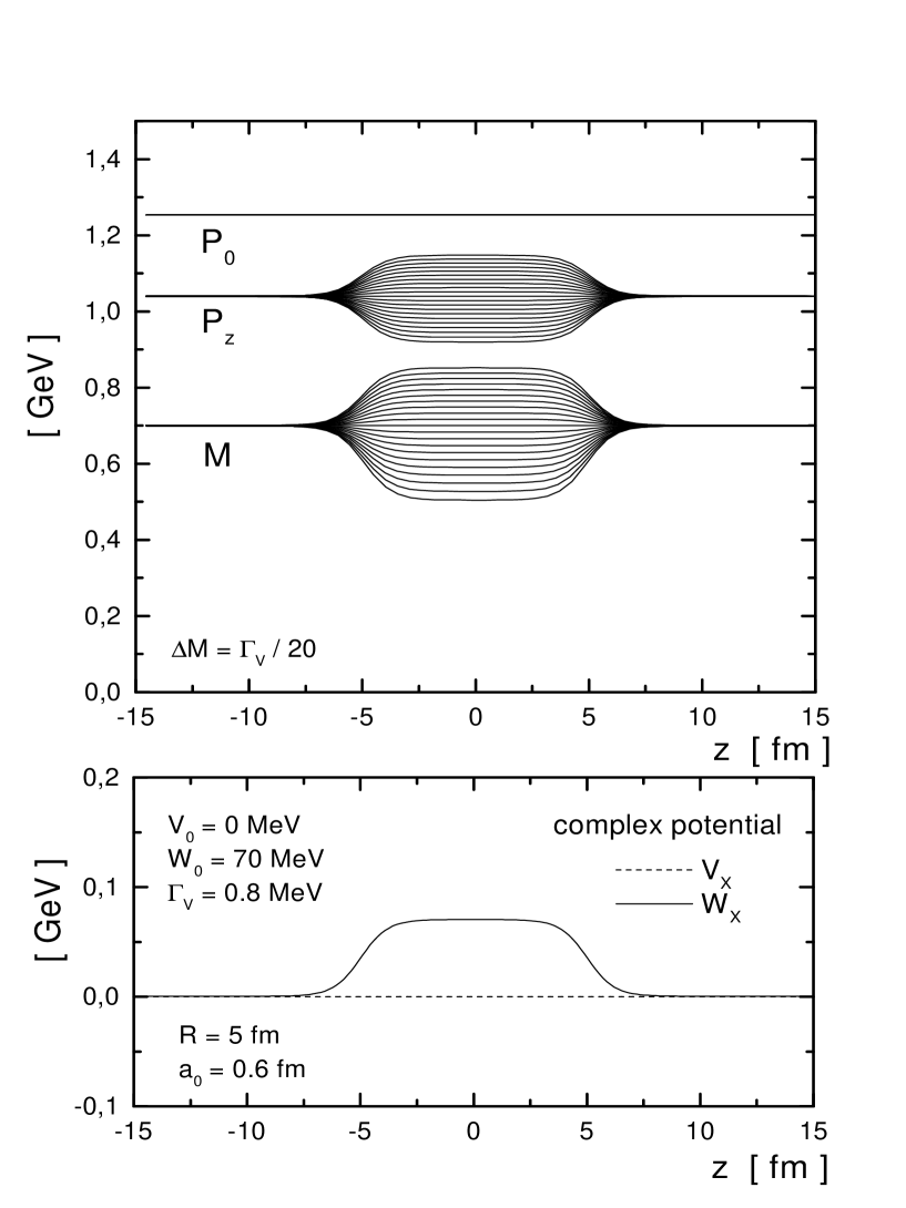
Figure 1: upper part: $P_{i0}$, $M_{i}$ and $P_{iz}$ as a function of $z(t)$ for a purely imaginary potential $W_{0}(t)=W_{0}=70$ MeV (lower part). The vacuum width is $\Gamma_{V}=0.8$ MeV and the initial separation in mass of the testparticles is given by $\Delta M=0.05\cdot\Gamma_{V}$.

In Fig. 1 (upper part) the results for $P_{i0}(z(t))$, $M_{i}(z(t))$ and $P_{iz}(z(t))$ are diplayed as a function of $z(t)$ instead of the time t. We show the evolution of 21 testparticles with mass parameters that are initially seperated by $\Delta M=0.05\cdot\Gamma_{V}$ in the case of a nonvanishing imaginary part of the potential ($W_{0}(t)=W_{0}=70$ MeV, $\Gamma_{V}=0.8$ MeV) but vanishing real part of the potential ($V_{0}=0$ MeV) (see Fig. 1 (lower part)). One recognizes that the differences between the mass parameters increase when reaching the potential region, which corresponds directly to a broadening of the spectral function. The same spreading behavior is observed for the three-momentum of the testparticles, such that the energy $P_{0}$ is conserved throughout the whole calculation (upper line). When leaving the potential region the splitting decreases and the correct asymptotic solution is restored.

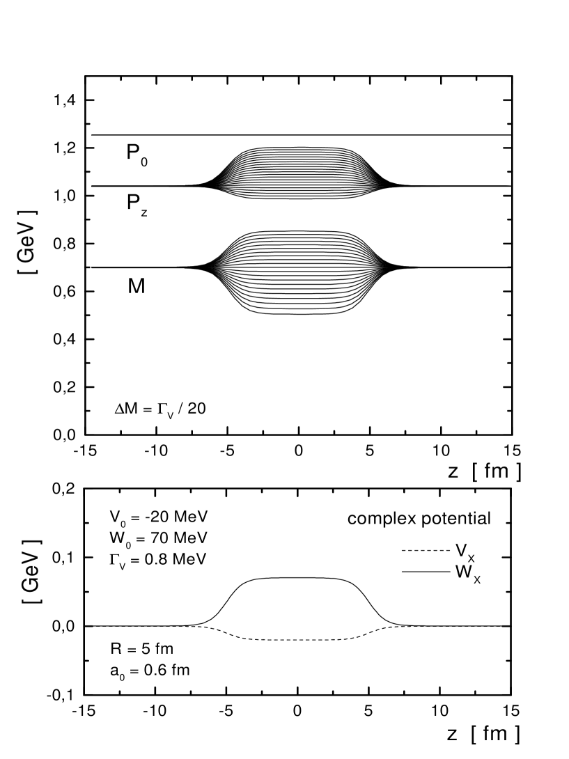
Figure 2: upper part: $P_{i0}$, $M_{i}$ and $P_{iz}$ as a function of $z(t)$ for a complex potential with $V_{0}=-20$ MeV, $W_{0}(t)=W_{0}=70$ MeV (lower part). For the vacuum width and the initial mass separation we have used the same values as in Fig. 1.

At next we present in Fig. 2 (upper part) a calculation where we additionally allow for a nonvanishing real part of the potential (i.e. $V_{0}=-20$ MeV, Fig. 2 (lower part)). While the spreading of the mass parameter is not affected by this change, we find a shift of the testparticle momenta where the real part of the potential deviates from zero since here the particles are accelerated.

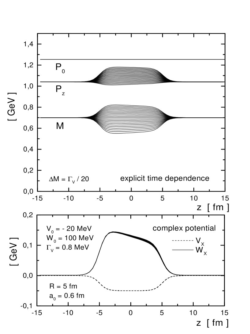
Figure 3: upper part: $P_{i0}$, $M_{i}$ and $P_{iz}$ as a function of $z(t)$ for an explicitly time-dependent imaginary part of the potential $W_{0}(t)=100$ MeV $(1-0.02\,c/$fm$\cdot t)$. The real part is taken as in Fig. 2 (lower part). For the vacuum width and the initial mass seperation we have used the same values as in Fig. 1.

While we up to now have only considered constant potentials in time, we now introduce an explicit time dependence corresponding to $W_{0}(t)=100$ MeV $(1-0.02\,c/$fm$\cdot t)$. As a result the spatial reflection symmetry vanishes for $P_{iz}(z(t))$ and $M_{i}(z(t))$ (cf. Fig. 3). For the given time dependence the mass splitting is smaller for given $z$ compared to a time-independent potential. As in the former cases here also the correct free solution is obtained for large $z$ while the energy is strictly conserved, too.

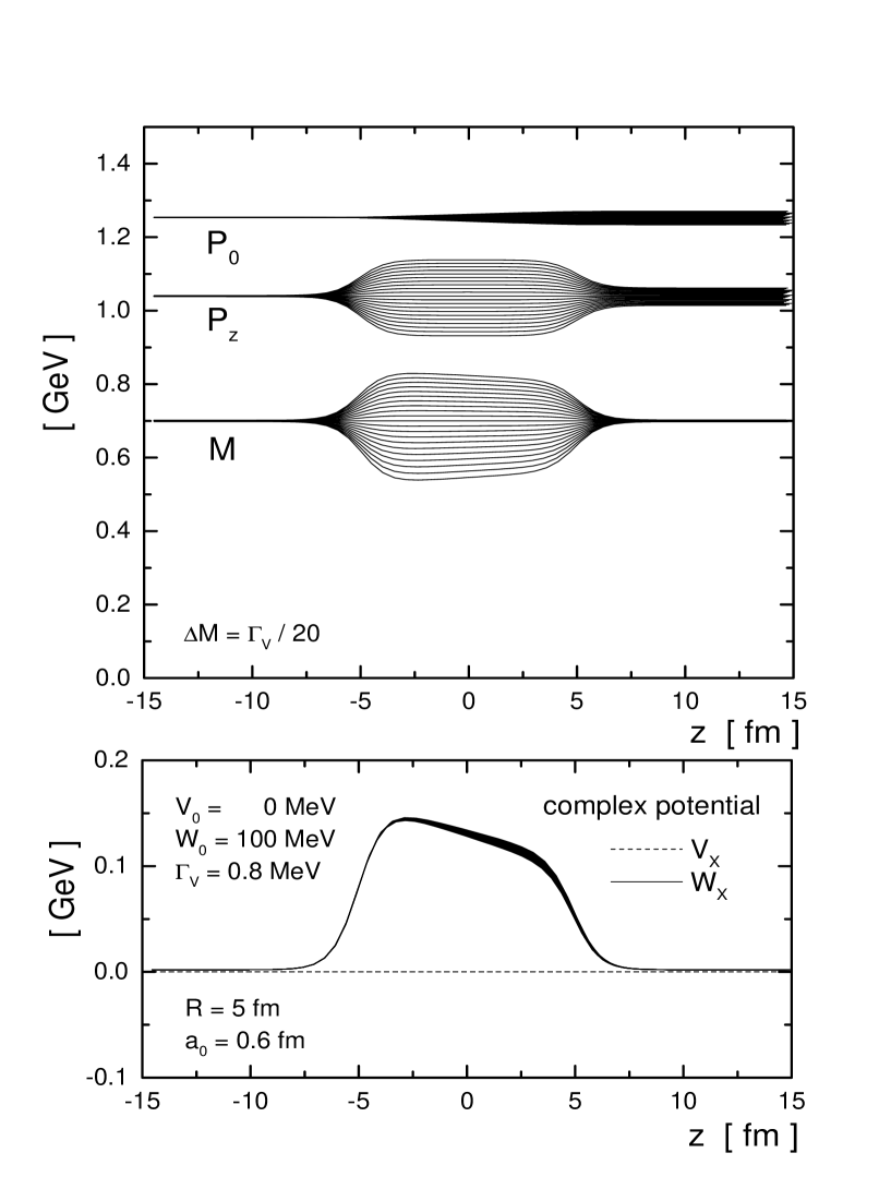
Figure 4: $P_{i0}$, $M_{i}$ and $P_{iz}$ as a function of $z(t)$ for the same time-dependent imaginary part of the potential $W_{0}(t)$ as in Fig. 3 but discarding the term $\sim\partial\Gamma_{X}/\partial t$ in eq. (44).

In order to discuss the effect of the additional term $\sim\partial\Gamma_{X}/\partial t$ introduced in eq. (44) we solve eqs. (39) - (41) that directly stem from the testparticle ansatz (38) for the model case presented in Fig. 3. The corresponding results in Fig. 4 show that the time evolution in $M^{2}$ is hardly effected, however, the individual trajectories spread out in energy $P_{0}$ which can be traced back to an asymptotic spread in momentum $P_{z}$. When integrating over the particle spectral function it can be shown that the total energy of the particle – which corresponds to a quantum mechanical state – is conserved again due to the symmetry of the spectral function in $(M^{2}-M_{0}^{2})$ for a local width $\Gamma_{X}$. Thus the original equations of motion (39) - (41) conserve energy with respect to the quantum mechanical state. However, within semiclassical transport simulations the spectral function will not be populated symmetrically around $M_{0}^{2}$ due to energy constraints, e.g. in reactions $pp\rightarrow pp\rho^{0}$ with invariant energy $\sqrt{s}\leq 2M_{p}+M^{\rho}_{0}$. Thus only the low mass fraction of the Breit-Wigner distribution will be populated for which the energy is no longer conserved throughout the propagation which might produce artefacts in further inelastic reaction channels. Such artefacts do not occur in a fully quantum mechanical theory due to the phase coherence $\sim iP_{0}t$ which guarantees energy conservation for $t\rightarrow\infty$. Since semiclassical transport simulations do not involve such phase coherence and thus violate the uncertainty relation with respect to energy and time, we have restored energy conservation locally in eqs. (43) - (45) for each testparticle representing a tiny slice in $dM^{2}$ of the spectral function.

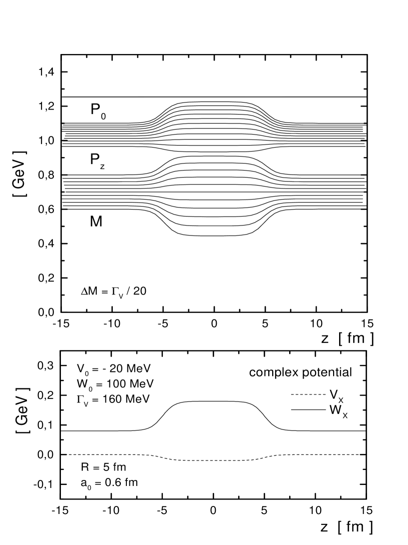
Figure 5: upper part: $P_{i0}$, $M_{i}$ and $P_{iz}$ as a function of $z(t)$ for a broad vacuum spectral function in a time-independent potential $V_{0}=-20$ MeV, $W_{0}(t)=W_{0}=100$ MeV (lower part). We have chosen a vacuum width $\Gamma_{V}=160$ MeV and an initial mass seperation of $\Delta M=0.05\cdot\Gamma_{V}$ for the testparticle trajectories displayed.

In the next example of this model study we show in Fig. 5 (upper part) the case of a broad vacuum spectral function entering a (time-independent) nonrelativistic potential with $V_{0}=-20$ MeV and $W_{0}(t)=W_{0}=100$ MeV. The vacuum width is chosen as $\Gamma_{V}=160$ MeV, while 11 testparticle trajectories are shown with an initial separation of the masses $\Delta M=0.05\cdot\Gamma_{V}$. One observes that the spectral function is further broadened in the complex potential zone and reaches its inital dispersion in mass again after passing the diffractive and absorptive area.

The question remains if the testparticle distribution (38) reproduces the local splitting in mass as expected due to quantum mechanics, i.e. in our case a Breit-Wigner distribution (49) with a local width $\Gamma_{X}$ = 2 $W_{0}(z)+\Gamma_{V}$. This is demonstrated in Fig. 6 where we show the spectral function as a function of mass $M$ from the testparticle evolution at fixed coordinate $z$ in comparison to the quantum Breit-Wigner distribution with local width $\Gamma_{X}$ (full lines) for a pure imaginary potential with parameters $W_{0}$ = 50 MeV and vacuum width $\Gamma_{V}$ = 2 MeV. The differences from the exact results in Fig. 6 are practically not visible for all values of $z$ from - 8 fm to 8 fm. The width of the distribution increases from 1 MeV in the vacuum ($z=\pm$ 8 fm) to 102 MeV (= 2 $W_{0}$+ $\Gamma_{V}$) in the center of the absorptive potential ($z$ = 0). Thus our off-shell quasiparticle propagation is fully in line with the quantum mechanical result at least for quasi-stationary quantum states.

To summarize our model results for the simple complex potential of Woods-Saxon-type, we find that energy conservation is guaranteed during the propagation as well as that the correct asymptotic solutions for the spectral functions are restored. Furthermore, in the potential region we observe a broadening of the width of the spectral function due to the space-time dependent imaginary part of the potential in line with quantum mechanics.

4 Application to nucleus-nucleus collisions

Apart from the model studies performed in the previous Section it is of interest, if the ’off-mass-shell approach’ proposed here leads to observable consequences in actual experiments such as for nucleus-nucleus collisions. This implies to specify the collision term in eq. (29). A corresponding expression can be formulated in full analogy to Ref. [9] by giving explicit approximations for $\Sigma^{<}$ and $\Sigma^{>}$ and using detailed balance as

$$I_{coll}(X,\vec{P},M^{2})=Tr_{2}Tr_{3}Tr_{4}A(X,{\vec{P}},M^{2})A(X,{\vec{P}}_{2},M_{2}^{2})A(X,{\vec{P}}_{3},M_{3}^{2})A(X,{\vec{P}}_{4},M_{4}^{2})$$ (50)

$$\{|T(({\vec{P}},M^{2})+({\vec{P}}_{2},M_{2}^{2})\rightarrow({\vec{P}}_{3},M_{3}^{2})+({\vec{P}}_{4},M_{4}^{2}))|_{{\cal A,S}}^{2}\>\delta^{4}({P}+{P}_{2}-{P}_{3}-{P}_{4})$$

$$[N_{X{\vec{P}}_{3}M_{3}^{2}}N_{X{\vec{P}}_{4}M_{4}^{2}}{\bar{f}}_{X{\vec{P}},M^{2}}{\bar{f}}_{X{\vec{P}}_{2},M_{2}^{2}}-N_{X{\vec{P}}M^{2}}N_{X{\vec{P}}_{2}M_{2}^{2}}{\bar{f}}_{X{\vec{P}}_{3},M_{3}^{2}}{\bar{f}}_{X{\vec{P}}_{4},M_{4}^{2}}]\}$$

with

$${\bar{f}}_{X{\vec{P}}}=1+\eta N_{X{\vec{P}}}$$ (51)

and $\eta=\pm 1$ for bosons/fermions, respectively. The indices ${\cal A,S}$ stand for the antisymmetric/symmetric matrix element of the scattering amplitude $T$ in case of fermions/bosons. We note that in (50) we have neglected gradient terms which lead to nonlocal collision terms [35, 36, 38, 39, 40]. Their effect can additionally be taken into account following the suggestions of Ref. [40], but are discarded here for simplicity and transparency.
In eq. (50) the trace over particles 2,3,4 reads explicitly for fermions

$$Tr_{2}=\sum_{\sigma_{2},\tau_{2}}\frac{1}{(2\pi)^{4}}\int d^{3}P_{2}\,\frac{dM^{2}_{2}}{2\sqrt{{\vec{P}}_{2}^{2}+M^{2}_{2}}},$$ (52)

where $\sigma_{2},\tau_{2}$ denote the spin and isospin of particle 2. In case of bosons we have

$$Tr_{2}=\sum_{\sigma_{2},\tau_{2}}\frac{1}{(2\pi)^{4}}\int d^{3}P_{2}\,\frac{dP_{0,2}^{2}}{2},$$ (53)

since here the spectral function is normalized as

$$\int\frac{dP_{0}^{2}}{4\pi}A_{B}(X,P)=1$$ (54)

whereas for fermions we have

$$\int\frac{dP_{0}}{2\pi}A_{F}(X,P)=\frac{M_{0}}{\sqrt{{\vec{P}}^{2}+M^{2}_{0}}}.$$ (55)

It is easy to show that the collision term (50) leads to the proper Bose or Fermion equilibrium distributions for $t\rightarrow\infty$.
Neglecting the ’gain-term’ in eq. (50) one recognizes that the collisional width of the particle in the rest frame is given by

$$\Gamma_{coll}(X,\vec{P},M^{2})=Tr_{2}Tr_{3}Tr_{4}\;\{|T(({\vec{P}},M^{2})+({\vec{P}}_{2},M_{2}^{2})\rightarrow({\vec{P}}_{3},M_{3}^{2})+({\vec{P}}_{4},M_{4}^{2}))|_{{\cal A,S}}^{2}$$ (56)

$$A(X,{\vec{P}}_{2},M_{2}^{2})A(X,{\vec{P}}_{3},M_{3}^{2})A(X,{\vec{P}}_{4},M_{4}^{2})\delta^{4}(P+P_{2}-P_{3}-P_{4})\ N_{X{\vec{P}}_{2}M_{2}^{2}}{\bar{f}}_{X{\vec{P}}_{3}}{\bar{f}}_{X{\vec{P}}_{4}}\},$$

where as in eq. (50) local on-shell scattering processes are assumed. We note that the extension of eq.(50) to inelastic scattering processes (e.g. $NN\rightarrow N\Delta$) or ($\pi N\rightarrow\Delta$ ect.) is straightforward when exchanging the elastic transition amplitude $T$ by the corresponding inelastic one and taking care of Pauli-blocking or Bose-enhancement for the particles in the final state. We mention that for bosons we will neglect a Bose-enhancement since their actual phase-space density is small for the systems of interest.
For particles of infinite life time in vacuum – such as protons – the collisional width (56) has to be identified with half the imaginary part of the self-energy that determines the spectral function (49). Thus the transport approach determines the particle spectral function dynamically via (56) for all hadrons if the in-medium transition amplitudes $T$ are known. Since in binary collisions due to energy and momentum conservation – once the final masses are fixed – only the final scattering angle $\Omega=(\cos\theta,\phi)$ is undetermined we can replace the amplitude squared in (56) as

$$|T({\vec{q}})|_{{\cal A,S}}=\frac{4\pi^{2}}{\mu^{2}}\ \frac{d\sigma}{d\Omega}(\sqrt{s})$$ (57)

where ${\vec{q}}$ is the momentum transfered in the collision at invariant energy $\sqrt{s}$ and $\mu$ is the reduced mass of the scattering particles. The differential cross section $d\sigma/d\Omega$ or $T({\vec{q}})$ in principle should be evaluated in the Brueckner approach, however, in practice effective parametrizations are employed (see below).

4.1 Numerical realisation

The following dynamical calculations are based on the conventional HSD transport approach [13, 30], where for energies up to 100 A MeV (GANIL energies) essentially the nucleon degrees of freedom are important, since inelastic processes $NN\rightarrow N\Delta\rightarrow\pi N,\;\pi N\rightarrow\Delta$ are suppressed. We only briefly mention that the formation cross section in the reaction $NN\rightarrow N\Delta$ is evaluated with the total $\Delta$-width $\Gamma_{\Delta}^{tot}=\Gamma_{\Delta}^{\pi N}+\Gamma_{\Delta}^{coll}$ [41] and that in the decay channel $\Delta\rightarrow\pi N$ the final nucleon state is selected by Monte Carlo using the local spectral distribution (49).
Whereas the real part of the nucleon self-energy is determined as in Ref. [13] and includes an explicit momentum dependence of the scalar and vector self-energies for nucleons in order to qualify also for relativistic reactions, we have to describe in more detail the implementation of the off-shell dynamics induced by $\Gamma_{XP}=\Gamma_{coll}(X,{\vec{P}},M^{2})$. According to (56) the collisional width is explicitly momentum (and energy) dependent, which introduces much larger numerical efforts as for momentum-dependent real potentials. In view of the limited energy range addressed here and for the purpose of an exploratory study it is sufficient to consider a space-time dependent collisional width $\Gamma_{X}$ which is obtained by averaging (56) at each time-step ($\Delta t=0.5fm/c$) in each cell in coordinate space (of size 1$fm^{3}$),

$$\Gamma_{X}=\frac{1}{\rho(X)}\sum_{\sigma,\tau}\frac{1}{(2\pi)^{4}}\int d^{3}P\frac{dM^{2}}{2\sqrt{{\vec{P}}^{2}+M^{2}}}\Gamma_{X{\vec{P}}M^{2}}$$ (58)

with the local density

$$\rho(X)=\sum_{\sigma,\tau}\frac{1}{(2\pi)^{4}}\int d^{3}P\frac{dM^{2}}{2\sqrt{{\vec{P}}^{2}+M^{2}}}F_{X{\vec{P}}M^{2}}.$$ (59)

We note, that in order to achieve a numerically ’flat’ function $\Gamma_{X}$ in space and time, one has to consider averages over a large set of ensembles typically in the order of $10^{3}$ testparticles per nucleon. By storing $\Gamma_{X}$ on a 4-dimensional grid the space-time derivatives of $\Gamma_{X}$, that enter the equations of motion (43) - (45), can be evaluated in first or second order. We mention that the Gaussian smearing algorithm described in Ref. [9] leads to sufficiently stable results (see below).
The collisions of nucleons are described by the closest distance criterion of Kodama et al. [51] in the individual $NN$ c.m.s., i.e.

$$|{\vec{X}}_{1}-{\vec{X}}_{2}|\leq\sqrt{\sigma({\vec{P}}_{1}-{\vec{P}}_{2})/\pi}$$ (60)

using the Cugnon parametrizations [52] for the in-medium $NN$ cross section $d\sigma/d\Omega(\sqrt{s})$ and identifying (in the $NN$ c.m.s.)

$$s-4m_{N}^{2}=s-4M^{2}=4{\vec{P}}^{2},$$ (61)

where $m_{N}$ is the nucleon vacuum mass, $M$ the actual off-shell mass and $\sqrt{s}$ the invariant energy of a nucleon-nucleon collision in the vacuum with c.m.s. momentum ${\vec{P}}$.
According to eq. (50) the nucleons can change their virtual mass $M$ in the scattering process $1+2\rightarrow 3+4$, while keeping the energy and momentum balance. This process is technically handeled by selecting the final nucleon masses by Monte Carlo according to the local Breit-Wigner distribution. However, our Monte Carlo simulations showed that this change of virtuality for elastic collisions has a minor effect on the observables to be discussed below.
Apart from the description of particle propagation and rescattering the results of the transport approach also depend on the initial conditions, ${\vec{X}}_{i}(0),{\vec{P}}_{i}(0),M_{i}^{2}(0)$. In view of nucleus-nucleus collisions, i.e. two nuclei impinging towards each other with a laboratory momentum per particle $P_{lab}/A$, the nuclei can be considered as in their respective groundstate, which in the semiclassical limit is given by the local Thomas-Fermi distribution [9]. Additionally the virtual mass $M_{i}^{2}$ has been determined by Monte-Carlo according to the Breit-Wigner distribution (49) assuming an in-medium width $\Gamma_{0}$ = 1 MeV. For the vacuum width of the nucleons we have used $\Gamma_{V}$ = 1 MeV which implies that nucleons propagating to the continuum in the final state of the reaction achieve their vacuum mass on the 0.1 $\%$ level. We note in passing that for the initialization we additionally have required $P_{0i}<m_{N}$ (in the restframe of the nucleus) which due to energy conservation implies that particles cannot escape ’numerically’ from the nucleus in the groundstate.

4.2 Nucleus-nucleus collisions at GANIL energies

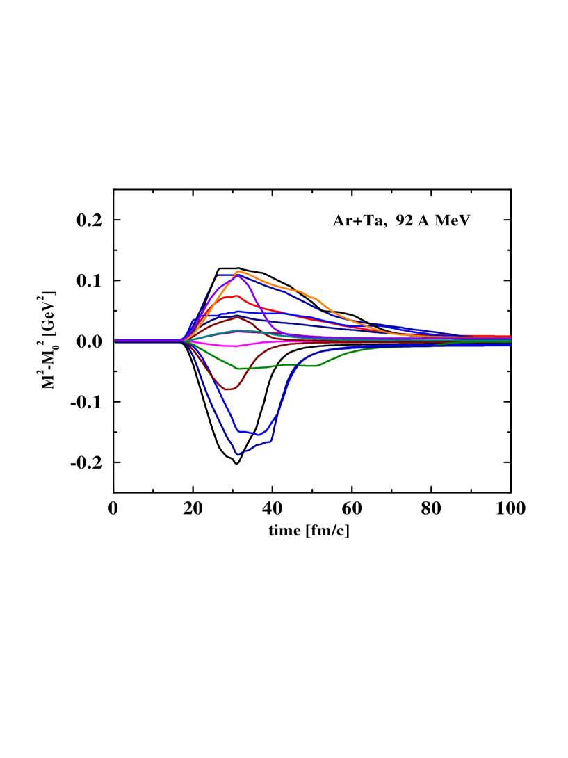
Figure 7: The off-shell propagation in mass ($M_{i}^{2}(t)-M_{0}^{2}$) as a function of time for 16 randomly chosen testparticles. The system is $Ar+Ta$ at 92 A MeV and impact parameter $b$ = 1 fm.

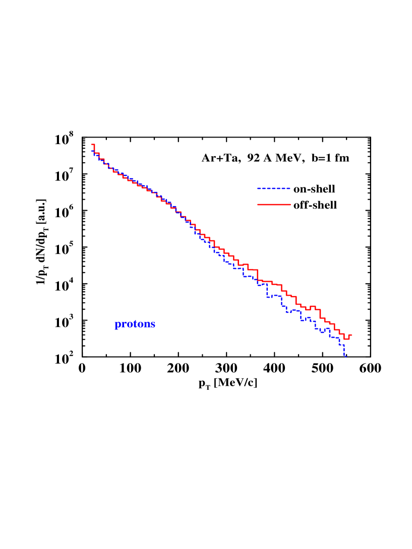
Figure 8: The transverse momentum spectra of protons for $Ar+Ta$ at 92 A MeV and impact parameter $b$ = 1 fm. The dashed histogram is the result from the on-shell propagation while the solid histogram is obtained including the off-shell propagation of nucleons.

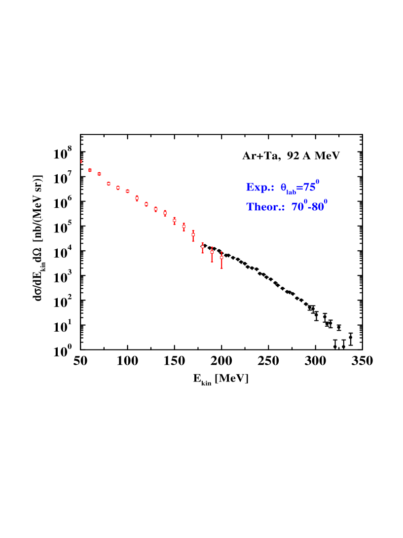
Figure 9: The inclusive kinetic energy spectra of protons for $Ar+Ta$ at 92 A MeV including the off-shell propagation in the transport approach (open squares) for $70^{0}\leq\theta_{lab}\leq 80^{0}$ in comparison to the experimental data from [46] (full circles).

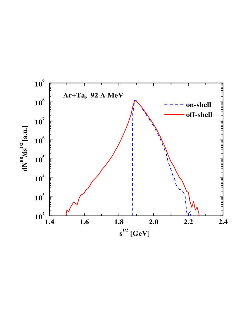
Figure 10: The number of baryon-baryon (BB) collisions as a function of the invariant energy $\sqrt{s}$ for $Ar+Ta$ at 92 A MeV integrated over all impact parameter. The solid line is obtained from including the off-shell propagation in the transport approach while the dashed line stands for the result in the on-shell limit.

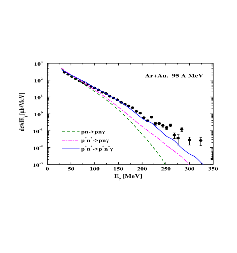
Figure 11: The inclusive differential photon spectra for $Ar+Au$ at 95 A MeV within various limits in comparison to the data from Ref. [47]. The dashed line is obtained in the on-shell propagation limit including on-shell nucleons in the final state, too. The dash-dotted line results from the off-shell propagation, however, including on-shell nucleons in the final production channel. The solid line results from the off-shell propagation of nucleons including also off-shell nucleons in the final channel.

Our first applications we devote to nuclear reactions at GANIL (92 - 95 A MeV) since here the more recent measurements have lead to conflicting results between different transport approaches [53]. We start with the reaction $Ar+Ta$ at 92 A MeV.
In view of Section 3 we present for some randomly chosen testparticles $i$ their off-mass-shell behaviour $M_{i}^{2}(t)-M_{0}^{2}$ as a function of time in a central collision ($b$ = 1 fm) in Fig. 7. It is seen that during the maximum overlap of the nuclei at $t\approx$ 30 fm/c the off-shellness reaches up to 0.2 GeV², however, in analogy to the model studies in Section 3 the nucleons become practically on-shell for $t\geq$ 90 fm/c. The finite width at the end of the calculation presented here is due to the fact that the collisional width $\Gamma_{coll}$ is still different from zero. The fluctuations in $M_{i}^{2}(t)-M_{0}^{2}$ in time give some idea about the numerical accuracy of the calculation for the space-time derivative of $\Gamma_{X}$; the functions become smoother when increasing the number of testparticles/nucleon furtheron $(\geq$ 1000).
Without explicit representation we note that the proton rapidity spectra $dN/dy$ do not change within the numerical accuracy when comparing the on-shell propagation limit with the results from the off-shell transport approach for $Ar+Ta$ at 92 A MeV. There is, however, a small enhancement in the proton transverse momentum spectra $1/p_{T}\,dN/dp_{T}$ for the off-shell propagation of nucleons as can be seen in Fig. 8, when the proton $p_{T}$ spectra are compared at an impact parameter $b$ = 1 fm.
The question remains, if such an enhancement might be seen experimentally or if the off-shell approach overpredicts the high momentum tail of the spectra. For this purpose we compare to the proton spectra from Ref. [46] taken at $\theta_{lab}$ = 75^o for kinetic energies above 175 MeV (Fig. 9). For this comparison we have integrated the proton spectra over all impact parameters with stepsize $\Delta b$ = 1 fm in the angular range $70^{o}\leq\theta_{lab}\leq 80^{0}$. The calculated spectra (open squares in Fig. 9) only extend up to 200 MeV due to statistics, however, match with the experimental data within the errorbars. A similar comparison has been performed by Germain et al. [53] where the traditional BUU and QMD calculations seem to be compatible with the experimental data within the statistics achieved whereas the Boltzmann Langevin (BL) calculations incorporating fluctuations in momentum space [34] overestimate the proton spectra by more than three orders of magnitude [53]. This rules out the latter BL approach but does not imply that our off-shell transport approach will properly describe the experimental spectra up to $E_{kin}$ = 350 MeV. In view of Fig. 9 the calculational statistics would have to be increased by more than 3 orders of magnitude which is unlikely to achieve for our present off-shell approach within a reasonable time due to the high amount of processor capacity needed. Note that due to nonlocal effects in the collision term the proton spectra might be slightly hardened additionally [40].
We thus continue with more qualitative investigations, that allow to extract the physics more clearly. In Fig. 10 we display the number of baryon-baryon collisions $dN^{BB}/d\sqrt{s}$ as a function of the invariant energy $\sqrt{s}$ for $Ar+Ta$ at 92 A MeV integrated over all impact parameters. The dashed line shows the result for the on-shell transport approach (starting at $2m_{N}$) whereas the solid line corresponds to the off-shell result, which extends down to $\sqrt{s}\approx$ 1.5 GeV. Note that elastic collisions of off-shell nucleons can occur due to their dynamical virtuality in mass. The dashed line is practically identical to the BUU calculations from Ref. [53] and is limited to collisions far below the kaon production threshold of $\sqrt{s_{0}}\approx$ 2.54 GeV. Thus the kaon production yield of (2.9$\pm 1.6)\cdot 10^{-9}b$ claimed in Ref. [48] for this system cannot be described in the on-shell limit, however, also not in our off-shell approach which shows only a small enhancement in the high $\sqrt{s}$ regime.
The latter $\sqrt{s}$ distribution can approximately be tested experimentally by hard photon spectra, a question that has been explored by the TAPS collaboration for $Ar+Au$ at 95 A MeV [47, 54]. In order to test our transport approach we have performed calculations for this system, too, using the parametrizations (4.13) of Ref. [9] for the elementary differential photon cross section in proton-neutron ($pn$) collisions. Note that the elementary photon bremsstrahlung in $pn$ collisions is at best known within a factor of 2 (cf. the discussion in Ref. [9]). Fig. 11 displays the results of our bremsstrahlung calculations in comparison to the data from Ref. [47]. The dashed line corresponds to the conventional on-shell calculation and is practically identical to the BUU analysis performed by Holzmann et al. [54], but underestimates the high energy photon yield dramatically. This situation does not improve very much when including the off-shell propagation of nucleons for the initial channel (dash-dotted line), however, still requiring that the nucleons in the final state are on-shell, too. Denoting off-shell nucleons by an extra ^∗ this corresponds to the individual reactions $p^{*}+n^{*}\rightarrow p+n+\gamma$, whereas the dashed line is obtained from the channel $p+n\rightarrow p+n+\gamma$.
On the other hand, the energetic photons are produced very early in the collision phase where the virtual mass distribution of nucleons – determined by $\Gamma_{X}$ (56) – becomes very broad. Thus including this virtuality in mass also in the final state, where the masses are selected by Monte-Carlo according to (49) with a local width $\Gamma_{X}$, we selfconsistently can sum the individual channels $p^{*}+n^{*}\rightarrow p^{\prime*}+n^{\prime*}+\gamma$. The result of such calculations is shown in Fig. 11 by the solid line which comes quite close to the experimental data [47]. We note that in the latter calculations we have averaged the photon yield over 10 MeV bins to reduce the statistical fluctuations emerging from the Monte-Carlo final state selection. Whereas in Ref. [54] the high energy photon yield has been tentatively attributed to very high momentum components in the initial phase-space distribution - which semiclassically are not bound - our present results indicate that this yield might be almost entirely explained (without introducing any additional assumptions) by the off-shell transport approach. It is presently unclear, if the missing high energy photon yield should be attributed to three-body reaction channels [55, 56], to the contribution of the $\Delta\rightarrow\gamma N$ channel [57] or to the secondary $\pi N\rightarrow\gamma N$ channel [58, 59].
The question now arises if the kaon yield from Ref. [48] for $Ar+Ta$ at 92 A MeV might also be due to off-shell hadronic states in the final channel. We thus have performed calculations for this system again within the following assumptions: $\Gamma_{X}^{N}=\Gamma_{X}^{\Lambda}$ and $\Gamma_{X}^{K}$ = 0 since the $KN$ cross section is rather small [60]. The parametrisations for the elementary reactions $NN\rightarrow N\Lambda K$ and $\pi N\rightarrow K\Lambda$ have been adopted from Refs. [60, 61] where $K,\bar{K}$ production has been systematically investigated for nucleus-nucleus reactions in the SIS energy regime. In view of Fig. 11 the small enhancement of energetic collisions for off-shell nucleons in the entrance channel does not have a large effect on the kaon production cross section as in case of energetic photons (cf. Fig. 11), but the reduction of the threshold due to the virtuality in mass of the final nucleon and $\Lambda$ hyperon should have (cf. Fig. 11). Unfortunately, within the statistics achieved in our calculations we did not find any $K\Lambda$ production event such that we presently cannot provide a solid answer.
In order to obtain some upper estimate we parametrize the collisional distribution $dN^{pn}/d\sqrt{s}$ (cf. Fig. 10) for $pn$ collisions by an exponential tail

$$\frac{dN^{pn}}{d\sqrt{s}}\sim\exp\{-\frac{\sqrt{s}}{E_{0}}\}$$ (62)

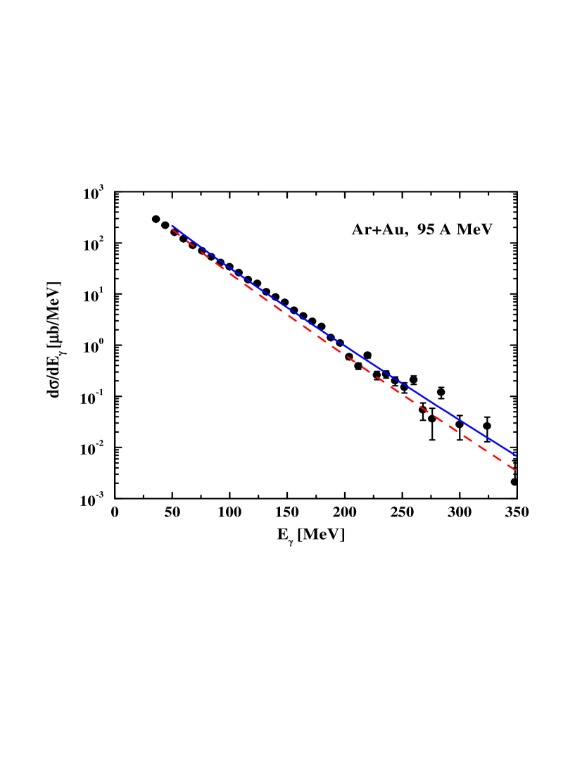
Figure 12: The inclusive differential photon spectra for $Ar+Au$ at 95 A MeV using the exponential $\sqrt{s}$ distribution (62) for $E_{0}$ = 33 MeV (dashed line) and $E_{0}$ = 35 MeV (solid line) in comparison to the data from Ref. [47].

with some slope parameter $E_{0}$ and fix the normalization constant as well as $E_{0}$ by the $\gamma$ spectra from the TAPS collaboration. The result of this model study is shown in Fig. 12 where the computed photon spectra for $E_{0}$ = 33 MeV (dashed line) and $E_{0}=$ 35 MeV (solid line) are shown in comparison to the data [47]. We note that within this model the photon spectra remain roughly exponential up to 700 MeV photon energy, which would have to be proven by experiment explicitly.
Now replacing the elementary differential photon cross section $d\sigma_{pn\rightarrow pn\gamma}(\sqrt{s})/d\Omega$ by the elementary kaon production cross section $d\sigma_{NN\rightarrow K\Lambda N}(\sqrt{s})$ [60] and correcting for isospin we obtain an inclusive kaon production cross section $\sigma_{K}\approx 1.6\cdot 10^{-11}b$ ($E_{0}=33$ MeV) and $\approx 6\cdot 10^{-11}b$ ($E_{0}=35$ MeV) for $Ar+Ta$ at 92 A MeV, which is about two orders of magnitude smaller than the cross section from Ref. [48]. Moreover, a note of caution has to be added here: In view of the analysis in Refs. [13, 62, 60, 61, 63, 64] the kaon potential in the nuclear medium is most likely repulsive and the $\Lambda$ potential only 2/3 of the nucleon potential. This shift in production threshold to higher $\sqrt{s}$ due to the real part of the hadron self-energies makes kaon production even more unlikely. We thus do not expect to describe the kaon cross section from Ref. [48] in our off-shell approach even when increasing the statistics by some orders of magnitude.

5 Summary

In this work we have derived and developed a semiclassical transport approach that in first order in the gradient expansion describes the virtual propagation of particles in the invariant mass squared $M^{2}$ besides the conventional propagation in the mean-field potential given by the real part of the self-energy. The derivation has been based on the familiar Kadanoff-Baym equations [14] by exploiting the relations between the different Green functions and the relations between their real and imaginary parts. Whereas in conventional transport approaches the imaginary part of the self-energy is reformulated in terms of a collision integral and simulated by on-shell binary collisions, we additionally account for the off-shell propagation of particles due to the imaginary part of the self-energy in eqs. (43) - (45). We note that in our formulation the single-particle energy $P_{0}$ is fixed by eq. (36) and that the propagation is determined by $dP_{0}/dt$ = 0 in the collisionless limit (if $Re\Sigma_{X}^{ret}$ has no explicit time dependence). On the other hand, the local collision rate $\Gamma_{X}$ is determined by the collision integrals themselves and can be used in transport approaches without introducing any new assumptions or parameters. In our present approach we have restricted to momentum-independent imaginary self-energies; an extension to the general case appears straight-forward according to Section 2, however, is numerically much more involved.
As a first application we have studied the dynamical evolution of particles in a fixed complex potential – having some similarities to hadron-nucleus collisions without explicit collisions – and demonstrated the off-mass-shell propagation in a transparent way for a variety of model cases. As also shown numerically, the energy conservation strictly holds for the set of eqs. (43) - (45). Furthermore, a distribution of off-shell particles regains its vacuum spectral function when moving out of the complex scattering centre; particles with vanishing (or very small) width become asymptotically on-shell again as required by the quantum mechanical boundary conditions while in the absorptive medium the spectral function reproduces the correct width in line with quantum mechanics (cf. Fig. 6).
We have, furthermore, presented the first dynamical calculations of the novel transport theory for nucleus-nucleus collisions at GANIL energies where we can test its results in comparison to experimental data. We find that the off-shell propagation of nucleons practically does not change the rapidity distributions $dN/dy$ and only has a moderate effect on the high transverse momentum spectra of protons. The latter we found to be fully compatible with the data from Ref. [46] for $Ar+Ta$ at 92 A MeV contrary to the Boltzmann-Langevin (BL) calculations in Ref. [53]. The distribution of nucleon-nucleon collisions in the invariant energy $\sqrt{s}$ is found to be also slightly enhanced for high invariant energies (as well as below the 2 nucleon threshold), which has some effect on the production of high energy $\gamma$-rays. Here we controlled our calculations by the photon data from the TAPS collaboration for $Ar+Au$ at 95 A MeV [47] that could be reasonably described in the off-shell limit when including especially the nucleon spectral functions in the exit channel $p^{*}+n^{*}+\gamma$. We have argued that this might be a first experimental indication for the off-shell propagation of nucleons that has to occur due to quantum mechanics. Our attempt to calculate the kaon cross section for $Ar+Ta$ at 92 A MeV [48] within the same line failed due to the limited statistics. However, when extrapolating the collisional $\sqrt{s}$ distribution by an exponentail tail (62) and fixing the slope parameter by the photon data from the TAPS collaboration [47] our upper limit for this cross section is roughly two orders of magnitude below the experimental value, which implies that the data point [48] remains ununderstood theoretically furtheron.
The actual applications of the present off-shell transport approach are not limited to nuclear physics problems, but should be of relevance for any system including particles of finite life time and/or high collision rates. The more practical point is now to set up new numerical recipies to increase statistics and also to include the explicit momentum dependence stemming from the imaginary part of the particle self-energy.

The authors like to acknowledge stimulating discussions with C. Greiner and S. Leupold throughout this study. Furthermore, they like to thank R. Holzmann for providing the data from Ref. [47] in electronic form and for valuable explanations of the TAPS experiment.

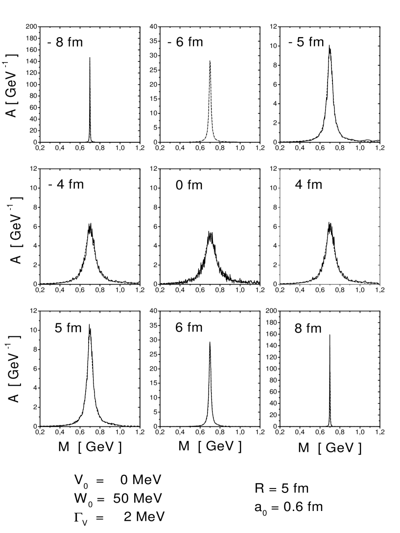
Figure 6: The spectral distribution at different coordinates $z$ from the testparticle distribution in comparison to the analytical result (solid lines) for $V_{0}$ = 0, $W_{0}$ = 50 MeV and $\Gamma_{V}$ = 2 MeV. The analytical result is practically identical to the histograms from the testparticle distribution and thus hardly visible.

References

- [1] J. Schwinger, J. Math. Phys. 2 (1961) 407.
- [2] S. J. Wang and W. Cassing, Ann. Phys. (N.Y.) 159 (1985) 328.
- [3] W. Cassing and S. J. Wang, Z. Phys. A 337 (1990) 1.
- [4] K. Chou, Z. Su, B. Hao, and L. Yu, Phys. Rep. 118 (1985) 1.
- [5] S. Mrówczyński and P. Danielewicz, Nucl. Phys. B 342 (1990) 345.
- [6] S. Mrówczyński and U. Heinz, Ann. Phys. (N.Y.) 229 (1994) 1.
- [7] H. Stöcker and W. Greiner, Phys. Rep. 137 (1986) 277.
- [8] G. F. Bertsch and S. Das Gupta, Phys. Rep. 160 (1988) 189.
- [9] W. Cassing, V. Metag, U. Mosel, and K. Niita, Phys. Rep. 188 (1990) 363.
- [10] W. Cassing and U. Mosel, Prog. Part. Nucl. Phys. 25 (1990) 235.
- [11] A. Faessler, Prog. Part. Nucl. Phys. 30 (1993) 229.
- [12] S. Bass, M. Belkacem, M. Bleicher et al., Prog. Part. Nucl. Phys. 41 (1998) 255.
- [13] W. Cassing and E. L. Bratkovskaya, Phys. Rep. 308 (1999) 65.
- [14] L. P. Kadanoff and G. Baym, Quantum statistical mechanics, Benjamin, New York, 1962.
- [15] P. Danielewicz, Ann. Phys. (N.Y.) 152 (1984) 239; ibid. 305.
- [16] W. Botermans and R. Malfliet, Phys. Rep. 198 (1990) 115.
- [17] R. Malfliet, Prog. Part. Nucl. Phys. 21 (1988) 207.
- [18] P. A. Henning, Nucl. Phys. A 582 (1995) 633; Phys. Rep. 253 (1995) 235.
- [19] C. Greiner and S. Leupold, Ann. Phys. (N.Y.) 270 (1998) 328.
- [20] S. J. Wang, W. Zuo and W. Cassing, Nucl. Phys. A 573 (1994) 245.
- [21] W. Cassing, K. Niita and S. J. Wang, Z. Phys. A 331 (1988) 439.
- [22] R. Fauser and H. Wolter, Nucl. Phys. A 584 (1995) 604.
- [23] C. M. Ko and G. Q. Li, J. Phys. G: Nucl. Part. Phys. 22 (1996) 1673.
- [24] J. Aichelin, Phys. Rep. 202 (1991) 233.
- [25] G. Q. Li, A. Faessler, and S. W. Huang, Prog. Part. Nucl. Phys. 30 (1993) 159.
- [26] C. Grégoire, B. Remaud, F. Sebille, L. Vinet, and Y. Raffray, Nucl. Phys. A 465 (1987) 317
- [27] H. Sorge, H. Stöcker, and W. Greiner, Ann. Phys. 192 (1989) 266.
- [28] B. A Li and C. M. Ko, Phys. Rev. C 52 (1995) 2037.
- [29] S. H. Kahana, D. E. Kahana, Y. Pang, and T. J. Schlagel, Annu. Rev. Nucl. Part. Sci. 46 (1996) 31.
- [30] W. Ehehalt and W. Cassing, Nucl. Phys. A 602 (1996) 449.
- [31] S. Ayik and C. Grégoire, Nucl. Phys. A 513 (1990) 187.
- [32] J. Randrup and B. Remaud, Nucl. Phys. A 514 (1990) 339.
- [33] G. F. Burgio and Ph. Chomaz, Nucl. Phys. A 529 (1991) 157.
-
[34]
E. Suraud, S. Ayik, M. Belkacem and J. Stryjewski,
Nucl. Phys. A 542 (1992) 141;
M. Belkacem, E. Suraud and S. Ayik, Phys. Rev. C 47 (1993) R16;
Y. Abe, S. Ayik, P.-G. Reinhard, and E. Suraud, Phys. Rep. 275 (1996) 49. - [35] R. Malfliet, Nucl. Phys. A 545 (1992) 3.
- [36] R. Malfliet, Phys. Rev. B 57 (1998) R11027.
- [37] P. Danielewicz and S. Pratt, Phys. Rev. C 53 (1996) 249.
- [38] V. Spicka, P. Lipavsky and K. Morawetz, Phys. Rev. B 55 (1997) 5095; Phys. Lett. A 240 (1998) 160.
- [39] P. Lipavsky, V. Spicka and K. Morawetz, Phys. Rev. E 59 (1999) 1291.
- [40] K. Morawetz, V. Spicka, P. Lipavsky, and Ch. Kuhrts, nucl-th/9902008.
- [41] W. Ehehalt, W. Cassing, A. Engel, U. Mosel, and Gy. Wolf, Phys. Rev. C 47 (1993) R2467.
- [42] M. Effenberger, E. L. Bratkovskaya and U. Mosel, nucl-th/9903026.
- [43] R. Rapp, G. Chanfray and J. Wambach, Nucl. Phys. A 617 (1997) 472.
- [44] G. E. Brown and M. Rho, Phys. Rev. Lett. 66 (1991) 2720.
- [45] W. Cassing, E. L. Bratkovskaya, R. Rapp and J. Wambach, Phys. Rev. C 57 (1998) 916.
- [46] M. Germain et al., Nucl. Phys. A 620 (1997) 81.
- [47] R. Holzmann et al., Phys. Rev. Lett. 72 (1994) 1608.
- [48] F. R. Lecolley et al., Nucl. Phys. A 583 (1995) 379c.
- [49] L. V. Keldysh, Zh. Eksper. Teoret. Fiz. 47 (1964) 1515; Sov. Phys. JETP 20 (1965) 1018.
- [50] B. D. Serot and J. D. Walecka, Adv. Nucl. Phys. 16 (1986) 1.
- [51] T. Kodama, S.B. Duarte, K.C. Chung, R. Donangelo, R.A.M.S. Nazareth, Phys. Rev. C 29 (1984) 2146.
- [52] J. Cugnon, D. Kinet and J. Vandermeulen, Nucl. Phys. A 379 (1982) 553.
- [53] M. Germain, Ch. Hartnack, J. L. Laville, J. Aichelin, M. Belkacem, and E. Suraud, Phys. Lett. B 437 (1998) 19.
- [54] R. Holzmann et al., Proc. of the 7th International Conference on Nuclear Reaction Mechanisms, Varenna, June 6-11, 1994, ed. by E. Gadioli, p. 261.
- [55] A. Bonasera, F. Gulminelli and J. Molitoris, Phys. Rep. 243 (1994) 1.
- [56] A. Bonasera and F. Gulminelli, Phys. Lett. B 259 (1991) 399; B 275 (1992) 24.
- [57] M. Prakash, P. Braun-Munzinger, J. Stachel and N. Alamanos, Phys. Rev. C37 (1988) 1959.
- [58] K. K. Gudima et al., Phys. Rev. Lett. 76 (1996) 2412.
- [59] G. Martinez et al., Preprint SUBATECH 1999.
- [60] W. Cassing, E. L. Bratkovskaya, U. Mosel, S. Teis, and A. Sibirtsev, Nucl. Phys. A 614 (1997) 415.
- [61] E. L. Bratkovskaya, W. Cassing and U. Mosel, Nucl. Phys. A 622 (1997) 593.
- [62] J. Schaffner-Bielich, I. N. Mishustin and J. Bondorf, Nucl. Phys. A 625 (1997) 325.
- [63] G. Q. Li, C.-H. Lee and G. E. Brown, Nucl. Phys. A 625 (1997) 372.
- [64] T. Waas, N. Kaiser, and W. Weise, Phys. Lett. B 379 (1996) 34.