Bulk properties of rotating nuclei and the validity of the liquid drop model at finite angular momenta

Abstract

Out of self-consistent semi-classical calculations performed within the so-called Extended Thomas-Fermi approach for 212 nuclei at all even angular momentum values $I$ ranging between 0 and 80 $\hbar$ and using the Skyrme SkM^∗ effective force, the $I$-dependence of associated liquid drop model parameters has been studied. The latter have been obtained trough separate fits of the calculated values of the strong interaction as well as direct and exchange Coulomb energies. The theoretical data basis so obtained, has allowed to make a rough quantitative assessment of the variation with I of the usual volume and surface energy parameters up to spin of $\sim 30$-40 $\hbar$. As a result of the combined variation of the surface and Coulomb energies, it has been shown that this $I$-dependence results in a significant enhancement of the fission stability of very heavy nuclei, balancing thus partially the well-known instability due to centrifugal forces.

1 Introduction

The availability of heavy ion beams at sufficiently high energy has made it possible to transfer very high angular momenta to nuclei, particularly in fusion-evaporation channels. Upon increasing the angular momentum one has opened up the exploration of a wide range of very large nuclear deformations, as in superdeformed states which were previously reached only in the fission process of ground (or weakly excited) states of heavy nuclei. As a matter of fact, one is currently able to reach the critical angular velocity regimes where the nuclear system experiences a centrifugal disassembly on all the accessible part of the nuclear chart. This is why a long time ago already, various authors have studied the equilibrium shapes and stability properties of rotating nuclei within a liquid drop model approach, drawing a close analogy between the properties of such a self-bound mesoscopic system with those of self-gravitating and rotating celestial objects (see Ref. [1] and Refs. quoted therein). Later, a more microscopic description of such nuclear systems has been provided upon minimizing the so-called “Routhian” variational quantity in a macroscopic-microscopic approach (from the pioneering works of Refs. [2, 3] to more systematic approaches as e.g. in Ref. [4]) thus relying again on the liquid drop model assumption when using in practice the Strutinsky energy expansion [5] in a slightly, and easily, transposed version. More recently, fully self-consistent Routhian approaches (after preliminary attempts making use of an inert core approximation [6, 7]), have been made available either with the Skyrme [8, 9, 10, 11] or the Gogny [12, 13] parameterization of the nucleon-nucleon effective interaction and have been shown to be reasonably realistic.

While the latter type of calculations does not imply any liquid drop model assumption to study the behavior of rotating nuclei, they are not really easy to handle in systematic calculations and certainly not suited, due to shell effects, to provide a transparent account of the bulk properties of nuclei at finite angular momenta. Yet, one would like to take stock on the impressive ability of such effective force parameterizations (Skyrme SkM^∗ [14] or SLy4 [15] and Gogny D1S [16] interactions) to yield a good reproduction of a wide array of static and (low excitation energy) dynamical properties. As well known, the theoretical framework to search for the bulk nuclear properties embedded in such purely microscopic approaches is a semi-classical approach à la Wigner [17], i.e. performing a truncated expansion of the solution (namely of the one-body reduced density matrix in the Hartree-Fock case). More specifically, we will use here the Extended Thomas-Fermi approach proposed in Ref. [18] and exhaustively discussed in Ref. [19].

In our Routhian approach we make use of a Skyrme type effective force parameterization. We explicitly express the functional dependence of some local density functions (as e.g. current and spin-vector densities) providing the relevant informations on the non-local (in $\boldsymbol{r}$) part of the time-odd component of the one-body density matrix, in terms of the spin-scalar density $\rho(\boldsymbol{r})$. Some steps in that direction have been made by Grammaticos and Voros both with [20] and without [21] spin degrees of freedom. However the full analytical solution of this problem has only been provided recently [22] and used to perform self-consistent semi-classical calculations [23]. The present description of bulk nuclear properties at finite angular momentum is clearly an extension of these previous studies. It fully develops some ideas presented earlier [23] in a somewhat exploratory fashion.

Indeed, we want to assess the relevance of the concept of a liquid drop for the description of rotating nuclei at equilibrium. The rationale for doing it stems from the anisotropic character of the rotational constraint imposed on the considered piece of nuclear matter which seems at first sight to be at variance with the isotropic character attached to a saturated liquid drop. Furthermore nuclei being leptodermous, as nicely illustrated by Myers and Swiatecki [24], one may wonder whether or not the surface tension, and hence the skin properties, might not be affected by the rotational character of the nuclear fluid. The above may be summarized in a practical form by recalling first that in Ref. [1], for instance, the nuclear energy is written, with usual notation, as

$$E(\beta,I)=E(\beta,I=0)+\frac{(I\hbar)^{2}}{2\Im^{(2)}},$$ (1)

where $\beta$ stands for a set of deformation parameters. One takes now for the energy $E(\beta,I=0)$ a standard version of the liquid drop model and the rigid body moment of inertia associated with the given shape for the parameter $\Im^{(2)}$. Therefore one assumes that all the $I$-dependence is only contained in the kinetic collective energy of a rigid rotation.

Let us translate that into the Hartree-Fock language. One may then split the total energy in the laboratory frame into two pieces:

$$E=E_{+}+E_{-},$$ (2)

the first involving only the part $\rho_{+}$ of the density matrix which is even with respect to the time-reversal symmetry and the second, $E_{-}$, issuing from the time-odd part $\rho_{-}$ of the density matrix (despite the two-body character of the interaction part of the Hamiltonian $H$, there are no cross-terms in Eq. (2) due to the time reversal invariance of $H$). For the standard Skyrme energy density functionals, the former part involves local densities (for both charge states) like the spin-scalar diagonal densities, the kinetic energy densities and the so-called spin-orbit densities (see e.g. Ref. [25]), while the latter involves the current densities and the spin-vector diagonal densities (see e.g. Ref. [9]). In the adiabatic limit, such a partition into two energies does correspond to the partition assumed in Eq. (1). In non-adiabatic regimes, the dependence of the two parts $\rho_{+}$ and $\rho_{-}$ of $\rho$ in terms of the collective velocity (in the present case the angular velocity $\omega$) is more complicated since $\rho_{+}$ may contain, for instance, a quadratic dependence on $\omega$.

One is thus lead, in practice to the two following questions:

– Is it correct that in a self-consistent semi-classical approach $E_{-}$ may be written as in Eq. (1) with a rigid body moment of inertia?
– Is it correct to assume that $E_{+}$ may be well approximated by a liquid drop energy, and if so are the parameters of this liquid drop independent on the angular momentum?

The answer to the first question is essentially affirmative as it has been demonstrated in Ref. [22]. There, it has been shown that the semi-classical moment of inertia $\Im$ may be split into two parts for which compact mathematical expressions have been given in the Skyrme force case. The first one is the zero order term of the semi-classical expansion (the so-called Thomas-Fermi term) and is as expected (and well known before the work of Ref. [22]) the rigid body moment of inertia. The remaining part corresponds to the second order term of this expansion which can be decomposed into two contributions, one coming from the orbital, the other from the spin degrees of freedom. They may be illustrated upon using a well established analogy between an angular velocity and a magnetic field $\boldsymbol{B}$ (analogy between, for instance, the Coriolis pseudo-force and the Lorentz magnetic force, first advocated in the context of a rotating many fermion system by Dabrowski [26]). For realistic effective forces (in Ref. [22], we have used the SkM^∗ force which is known to give, at least in the $\beta$-stability valley a very satisfactory account of bulk nuclear properties) one has found a negative contribution of the orbital degrees of freedom to $\Im$, corresponding to an analog of a Landau diamagnetism, while the spin degrees of freedom contribution being positive, corresponds to a Pauli paramagnetic alignment. Both contributions are rather weak with respect to the Thomas-Fermi contribution, and moreover, as we have seen, they cancel each other to a large extent. Specifically, it has been found in Ref. [22] that one can write with obvious notation for a nucleus of mass $A$

$$\Im=\Im_{RB}[1+(\eta_{l}+\eta_{s})A^{-2/3}]$$ (3)

with the following values for the coefficients of the second order contributions (again for the SkM^∗ force):

$$\eta_{l}\approx-1.94,\hskip 14.22636pt\eta_{s}\approx 2.63,$$ (4)

leaving thus only a small correction to the rigid body ansatz, especially for heavy nuclei.

The problem of the kinetic collective energy being settled, the second question raised above is still open. First, is there any $I$-dependence in the non-kinetic ($E_{+}$) part of the energy? The answer to this is clearly yes. In Ref. [23], we have found that the self-consistent semi-classical energy $E_{+}$, for a given nucleus and using the SkM^∗ force, was indeed very much varying. Therefore, if at all valid, the liquid drop model to be used should clearly incorporate coefficients varying with the rotational velocity. An important question needs to be clarified at this point. A priori, there are no clear reasons why the liquid drop parameters should vary with $I$ or $\omega$ . Of course, the former being an observable which is furthermore a conserved quantity, seems a better candidate. But it is not clear to us why this quantal feature should reflect itself in this way for the rotational dependence of a rather crude modelization of the energy. However in Ref. [23], it has been shown that the variation of the energies $E_{+}$ were of similar relative magnitude between light and heavy nuclei, only when compared for the same value of $I$ (and not for the same value of $\omega$ which scales as $A^{-5/3}$ for a given value of $I$). We are thus lead to conclude phenomenologically that, if valid, the rotating liquid drop model should be $I$-dependent and not $\omega$-dependent. (Note that even though, as stated above, the results of Ref. [23] may lead to such a conclusion, the liquid drop model parameter fit in terms of the angular velocity performed there is somehow inconsistent).

The remaining issue is then the validity of the liquid drop model at finite angular momenta. For that purpose, we need to perform for each value of the angular momentum which we decide to study, high accuracy self-consistent semi-classical calculations for a sufficient number of nuclei covering reasonably well the chart of nuclides so that we should be able to make a significant liquid drop parameter fit. This was not at all the case of the calculations of Ref. [23] (too few nuclei, 33, and an accuracy in the variational semi-classical solutions somewhat insufficient for the present purpose). It is the aim of the present paper therefore to achieve in a numerically satisfactory fashion the preliminary calculations sketched in Ref. [23].

Two remarks are worthwhile at this point. First, it is clear that we do not include pairing correlations. This could be done, as we are currently attempting, within the BCS or the Hartree-Fock-Bogoliubov framework in the semi-classical approximation (for the Thomas-Fermi and Extended Thomas-Fermi non-rotating case see Refs. [27] and [28] respectively). The second remark deals with the bulk deformation properties. All our self-consistent semi-classical calculations will be performed at sphericity. As a matter of fact when assessing the validity of a liquid-drop model approximation, one intends to do two different things. The first is to check the ability of a liquid drop parameterization to reproduce with a good accuracy the semi-classical energies at a given deformation. For that purpose choosing spherical solutions is an obvious choice for the sake of computational convenience. The second is to check whether or not the semi-classical energies are varying with deformation like a sum of various geometrical quantities associated with the deformation (surface, Coulomb energy or more). This will not be attempted here. Yet, we think obvious that the present approach casts some light on nuclear deformation properties at finite angular momentum (through the fissility parameter for instance). Restricting ourselves to spherical shapes, we may therefore ignore the difficulties described by Krappe, Nix and Sierk [29], and studied in the rotational context in Refs. [30, 31], when dealing with nuclear shapes having some concavity (like fission saddle points of some nuclei) or not simply connected (like post scission or fusion configurations, for instance).

The paper will be organized as follows. Section 2 will detail the theoretical framework in which we have studied the bulk rotational properties of the nuclei. In Section 3 we will present the calculational approach insisting on the choice of the sample of nuclei, the accuracy of the self-consistent calculations and the fitting procedure. The results will be displayed and discussed in Section 4. Finally, Section 5 will contain some conclusions and perspectives of the present work.

2 The theoretical framework

To describe in a semi-quantal way the wave function of a nucleus rotating with respect to the laboratory frame with an angular velocity $\omega$, one minimizes the Routhian $R$ defined in terms of the microscopic Hamiltonian $H$ as

$$R=H-\omega I.$$ (5)

In the Hartree-Fock approximation, the single particle states defining the solution is thus reduced to an eigenvalue problem involving the one-body reduction of the Routhian of Eq. (5). The corresponding semi-classical one-body density matrix may thus be obtained according to the usual Extended Thomas-Fermi method upon replacing the Hartree-Fock one-body Hamiltonian by the corresponding one-body Routhian. For a Skyrme effective force, the Routhian expectation value is obtained as an integral over space of a Routhian density which is expressed (see e.g. Ref. [9]) in terms of various densities (spin-scalar and spin-vector densities, kinetic energy densities, spin-orbit and current densities). In the semi-classical Extended Thomas-Fermi approach all densities may be expressed as functionals of the spin-scalar densities [22]. Therefore the Routhian density is itself a functional of the spin-scalar densities. The variational solution for a given angular velocity may be just obtained then by minimizing the integral of this Routhian functional.

To do so, choosing the $Oz$ axis as the rotation axis, we have used a parameterization of the density functions $\rho_{q}(\boldsymbol{r})$ (here called $\rho_{q}^{\mathrm{new}}$ for reasons explained below), where $q$ stands for the charge state, expressed in cylindric coordinates $(r,z,\varphi)$ as

$$\rho_{q}^{\mathrm{new}}(r,z)=\rho_{0q} \left[1-\alpha_{q}\exp(-\beta_{q}^{2}r^{2}s_{q}^{2/3})\right]$$ (6)

$$\left[1+\exp\left(\frac{\sqrt{r^{2}s_{q}^{2/3}+z^{2}s_{q}^{-4/3}}-R_{q}}{\sigma_{q}}\right)\right]^{-\gamma_{q}}.$$

Whereas we want to describe spherical solutions, they appear a priori to have only a cylindrical symmetry (see however the discussion below). The densities depend on 14 parameters (7 for each charge state). However the space integrals of the densities $\rho_{q}(\boldsymbol{r})$ should be equal to $N_{q}$, the particle number of charge $q$, leaving thus 12 independent parameters. For $\alpha_{q}=0$, and $s_{q}=1$, one is left with surface asymmetric (for $\gamma_{q}\neq 1$) Fermi distributions as widely used in Ref. [19] for instance

$$\rho_{q}(\boldsymbol{r})=\rho_{0q}\left[1+\exp\left(\frac{\sqrt{x^{2}+y^{2}+z^{2}}-R_{q}}{\sigma_{q}}\right)\right]^{-\gamma_{q}}.$$ (7)

One notices in Eq. (6) that in front of the modified Fermi term we have enclosed a factor similar to what has been considered in Ref. [19] with a very significant difference, namely its anisotropic character. This has been introduced to let the solution adjust to the centrifugal forces which are themselves not isotropic. For the same reasons advocated in the slightly different context of Ref. [19], we have reduced the variational space by imposing that $\beta_{q}$ should have a fixed value within a range where this modification would not alter the desired leptodermous and smooth character of the semi-classical densities. In practice we have used:

$$\beta_{q}^{2}=1/(c_{q}R_{q})^{2},\hskip 14.22636ptc_{q}=0.5,$$ (8)

$R_{q}$ being the radius parameter introduced in Eq. (6)

Let us discuss now the scaling parameter $s_{q}$ appearing in Eq. (6). Introducing an anisotropy as above described, our solution lacks its spherically symmetrical character. To be able to compare solutions with various values of the parameters $\alpha_{q}$ we must constrain them to keep, in some way, a vanishing deformation. This is achieved by imposing that

$$\langle r^{2}\rangle_{q}=2\langle z^{2}\rangle_{q},$$ (9)

where $\langle r^{2}\rangle_{q}$ and $\langle z^{2}\rangle_{q}$ stand for the expectation values of $r^{2}$ and $z^{2}$ for the distribution of nucleons of charge $q$. Taking into account the particle number conservation, one gets the following explicit expression for the parameter $s_{q}$:

$$s_{q}^{-2}=2\int_{0}^{\infty}r\;\mathrm{d}r\int_{-\infty}^{\infty}z^{2}\rho_{q}^{\mathrm{old}}\;\mathrm{d}z\;\left[\int_{0}^{\infty}r^{3}\;\mathrm{d}r\int_{-\infty}^{\infty}\rho_{q}^{\mathrm{old}}\;\mathrm{d}z\right]^{-1},$$ (10)

with

$$\rho_{q}^{\mathrm{old}}(r,z)=\rho_{0q}\left[1-\alpha_{q}\exp(-\beta_{q}^{2}r^{2})\right]\left[1+\exp\left(\frac{\sqrt{r^{2}+z^{2}}-R_{q}}{\sigma_{q}}\right)\right]^{-\gamma_{q}}.$$ (11)

To obtain the expression for $s_{q}^{2}$ one may introduce stretched coordinates $\tilde{r}=s_{q}^{1/3}r$ and $\tilde{z}=s_{q}^{-2/3}z$ in terms of which one has $\rho_{q}^{\mathrm{new}}(\tilde{r},\tilde{z})=\rho_{q}^{\mathrm{old}}(r,z)$.

The usual iterative procedure now begins with the determination of the scaling factor $s_{q}.$ Then we find the parameter $\rho_{0q}$ from the normalization condition

$$N_{q}=4\pi\int_{0}^{R\max}r\;\mathrm{d}r\int_{0}^{z_{\max}}\rho_{q}^{\mathrm{new}}(r,z)\;\mathrm{d}z,$$ (12)

Hereafter $N_{p}=Z,$ $N_{n}=N$. In all the integrals we take advantage of the reflexion symmetry $\rho_{q}^{\mathrm{new}}(r,-z)=\rho_{q}^{\mathrm{new}}(r,z)$ .

Once the variational parameters have been determined, one obtains the total energy in the laboratory frame according to the decomposition of Eq. (2) where $E_{+}$ is obtained by using the time-even energy Skyrme functional of Ref. [25]. One gets namely (see Ref. [22]).

$$E[\rho]=\int{\cal H}[\rho]\;\mathrm{d}^{3}r=\int{\cal H}_{\mathrm{stat}}[\rho]\;\mathrm{d}^{3}r+\frac{1}{2}\Im^{(2)}(\rho)\omega^{2},$$ (13)

with

$${\cal H}_{\mathrm{stat}}[\rho]=\frac{\hbar^{2}}{2m}\sum_{q}f_{q}\tau_{q}(\rho)+V_{q}^{\mathrm{central}}(\rho)+V_{q}^{\mathrm{s.o.}}(\rho),$$ (14)

where $f_{q}$ is the usual Skyrme effective mass factor and $\tau_{q}(\rho)$ the ETF expression for the static kinetic energy density up to $\hbar^{4}$-terms (see e.g. Ref. [19]). The expression for $V_{q}^{\mathrm{central}}(\rho)$ is given with the notation of Ref. [9] for the Skyrme parameters ($B_{i},\alpha$) where as a general rule all densities without a charge state subscript $q$ are total densities (i.e. for instance $\rho=\sum_{q}\rho_{q}$).

$$V_{q}^{\mathrm{central}} = B_{1}\rho^{2}+B_{2}\sum_{q}\rho_{q}^{2}+B_{5}\rho\nabla^{2}\rho+B_{6}\sum_{q}\rho_{q}\nabla^{2}\rho_{q}$$ (15)

$$+\big{(}B_{7}\rho^{2}+B_{8}\sum_{q}\rho_{q}^{2}\big{)}\rho^{\alpha}$$

The ETF expression for the spin-orbit contribution up to $\hbar^{4}$-terms $V_{q}^{\mathrm{s.o.}}$ to ${\cal H}_{\mathrm{stat}}(\rho)$ is given e.g. in Eq. (A5) of the review paper by Brack et al. [19]. Finally, the ETF expression of $\Im^{(2)}$ up to $\hbar^{2}$-terms has been derived in Ref. [22] (see e.g. Eq. (63) there).

To obtain solutions corresponding to precise values of the angular momentum $I$, we adjust iteratively the value of $\omega$ accordingly. We have made calculations for a sample of 212 even-even nuclei, covering all the chart of nuclides whose mass is higher than 34 within reasonable estimates of the two drip lines and including five long isotopic series (Ca, Ge, Sn, Sm, Pb), as detailed in Table 1. Obviously for semi-classical solutions whose static properties are smooth functions of $N$ and $Z$, the particular choice of nuclei is irrelevant provided that the sampling is dense enough in the region of interest for the properties under study. For instance to get reasonable estimates of proton-neutron asymmetry properties it is essential to include in the sample isotopes up to the drip lines. We will discuss in the next Section the quality of our sample in this respect.

Table 1: Isotopes used in the fit. For each elements we have considered all even-A isotopes from $A_{i}$ to $A_{f}$ (including the boundaries) corresponding to a number of isotopes $N_{\mathrm{is}}$.

Element	$Z$	$A_{i}$	$A_{f}$	$N_{\mathrm{is}}$		Element	$Z$	$A_{i}$	$A_{f}$	$N_{\mathrm{is}}$
Ca	20	34	78	23		Yb	70	166	180	8
Ni	28	56		1		Os	76	184	198	8
Ge	32	58	118	31		Pb	82	182	242	31
Zr	40	86	100	8		Th	90	226	240	8
Sn	50	94	168	38		Pu	94	236	252	9
Ce	58	134	148	8		Cf	98	252		1
Sm	62	120	194	38

Now, for each value of $I$, we have made a liquid drop model fit of the 212 nuclear energies $E_{\mathrm{nuc}}$, defined in terms of the energy $E_{+}$ as

$$E_{\mathrm{nuc}}=E_{+}-E_{\mathrm{coul}},$$ (16)

where $E_{\mathrm{coul}}$ is the total Coulomb energy. The latter includes the direct term ($E_{\mathrm{CD}}$) and the so-called “Slater approximation” (namely a local density approximation [32] of the Bethe-Bacher [33] nuclear matter estimate) for the exchange term ($E_{\mathrm{CE}}$) whose accuracy has been checked earlier [34]. Both Coulomb energy terms have been fitted separately (i.e. independently of each other and of the nuclear energy). We leave for another publication [35] an in-depth discussion of the liquid drop fit of the Coulomb energies, in particular its isospin-dependence which is generally overlooked (see a preliminary account of such a work in the review of Ref. [36]). Namely, the liquid drop expression for $E_{\mathrm{nuc}}$ which we have considered here, is given for the nucleus labeled by j ($j=1,\cdots N_{A}$, where $N_{A}$ is the number of nuclei entering the fit) as

$$E_{\mathrm{nuc}}^{j}(I) = a_{v}(I)\;\Big{[}1-k_{v}(I)(1-2Z_{j}/A_{j})^{2}\Big{]}\;A_{j}$$ (17)

$$+a_{s}(I)\;\Big{[}1-k_{s}(I)(1-2Z_{j}/A_{j})^{2}\Big{]}\;A_{j}^{2/3}.$$

The Coulomb part is the sum of a direct ($E_{\mathrm{CD}}$) and exchange ($E_{\mathrm{CE}}$) part whose absolute value is known to be one order of magnitude smaller than $E_{\mathrm{CD}}$ (see e.g. Ref. [34]). For the direct term we have made two fits one which is rather usual (sharp density term plus a leptodermous surface correction as in Ref. [37])

$$E_{\mathrm{CD}}^{j}(I)=c(I)\;Z_{j}^{2}/A_{j}^{1/3}-\gamma(I)\;Z_{j}^{2}/A_{j},$$ (18)

and another extended one discussed in a forthcoming paper [35] which takes into account both the surface diffuseness and $(N-Z)$ isotopic effects

$$E_{\mathrm{CD}}^{j}(I) = c(I)\;\Big{[}1+\alpha_{1}(I)\big{(}1-2Z_{j}/A_{j}\big{)}A_{j}^{-1/3}+\alpha_{2}(I)A_{j}^{-1/3}\Big{]}\;Z_{j}^{2}/A_{j}^{1/3}$$ (19)

$$-\gamma(I)\;\Big{[}1+\beta(I)\big{(}1-2Z_{j}/A_{j}\big{)}\Big{]}\;Z_{j}^{2}/A_{j}.$$

For the exchange term ($E_{\mathrm{CE}}$) we consider the usual exchange term deduced from an infinite nuclear matter non-diagonal density matrix [33]

$$E_{\mathrm{CE}}^{j}(I)=c^{\prime}(I)\;Z_{j}^{4/3}/A_{j}^{1/3}.$$ (20)

3 Some computational details

We use the SkM^∗ force with the original set of parameters previously determined by fitting HF results to experimental data. The fit of the effective interaction has been made correcting approximately the HF energy by subtracting only the one-body part of the mean energy of the center of mass (c.m.) motion, $E_{\mathrm{cm}}^{(1)}$ (see Sect. 2.3 of [38]). To be consistent, in our ETF calculations we will also only take into account that part of the c.m. energy correction. The introduction of this correction leads to the replacement of the nucleon mass $m$ by $mA/(A-1)$ in the total kinetic energy and so in our non-local case we have to replace $\sum_{q}f_{q}\tau_{q}(\rho)$ by $\sum_{q}f_{q}(1-1/A)\tau_{q}(\rho)$ in the energy density ${\cal H}[\rho]$ [see Eq. (14)].

The calculation of the Coulomb energy is the most time consuming part of the problem due to its range. We take into account both the direct and exchange parts of this energy:

$$E_{\mathrm{Coul}}=\frac{e}{2}\int\mathrm{d}^{3}r_{1}\;\rho_{p}(\boldsymbol{r}_{1})V_{C}(\boldsymbol{r}_{1})+E_{\mathrm{Coul}}^{\mathrm{exc}},$$ (21)

with

$$V_{C}(\boldsymbol{r}_{1})=e\int\mathrm{d}^{3}r_{2}\;\frac{\rho_{p}(\boldsymbol{r}_{2})}{\left|\boldsymbol{r}_{1}-\boldsymbol{r}_{2}\right|}.$$ (22)

The Coulomb exchange part is treated as already mentioned in the so-called “Slater approximation” [32, 33, 34]:

$$E_{\mathrm{Coul}}^{\mathrm{exc}}=-\frac{3e^{2}}{4}(3/\pi)^{1/3}\int\mathrm{d}^{3}r\;\rho_{p}^{4/3}(\boldsymbol{r}).$$ (23)

The integrand in the direct part of the Coulomb energy has a logarithmic singularity at the point $\boldsymbol{r}_{1}=\boldsymbol{r}_{2}$. Therefore such a formula is not suitable for numerical integration. A way to bypass the latter difficulty is to use the relation

$$\nabla_{\boldsymbol{r}_{2}}^{2}\left|\boldsymbol{r}_{1}-\boldsymbol{r}_{2}\right|=\frac{2}{\left|\boldsymbol{r}_{1}-\boldsymbol{r}_{2}\right|}$$ (24)

and to carry out two integrations by parts to get:

$$V_{C}(\boldsymbol{r}_{1})=\frac{e}{2}\int\mathrm{d}^{3}r_{2}\;\left|\boldsymbol{r}_{1}-\boldsymbol{r}_{2}\right|\nabla_{\boldsymbol{r}_{2}}^{2}\rho_{p}(\boldsymbol{r}_{2}).$$ (25)

With our parameterization (6) of the density it is most convenient to treat the problem in cylindrical coordinates choosing the axis of symmetry to be the $Oz$ axis. Integrating over the azimuthal angle $\varphi_{2}$ the expression for $V_{C}(r_{1},z_{1})$ reduces to [39]

$$V_{C}(r_{1},z_{1})=2e\int_{0}^{\infty}r_{2}\;\mathrm{d}r_{2}\int_{-\infty}^{\infty} \mathrm{d}z_{2}\;\sqrt{(z_{1}-z_{2})^{2}+(r_{1}+r_{2})^{2}}$$ (26)

$$E(k)\nabla^{2}\rho_{p}(r_{2},z_{2}),$$

with

$$k^{2}=4r_{1}r_{2}\big{[}(z_{1}-z_{2})^{2}+(r_{1}+r_{2})^{2}\big{]}^{-1}$$ (27)

and where $E(k)$ denotes the complete elliptic integral of the second kind:

$$E(k)=\int_{0}^{\pi/2}\sqrt{1-k\sin^{2}u}\;\mathrm{d}u.$$ (28)

We have therefore for the direct part of the Coulomb energy:

$$E_{\mathrm{Coul}}^{\mathrm{dir}}=\pi e\int_{0}^{\infty}r_{1}\;\mathrm{d}r_{1}\int_{-\infty}^{\infty}\mathrm{d}z_{1}\;\rho_{p}(r_{1},z_{1})V_{C}(r_{1},z_{1}).$$ (29)

In practice, the infinite limit of integration is replaced by $R=25$ fm, and we get

$$E_{\mathrm{Coul}}^{\mathrm{dir}}=4\pi e^{2}\rho_{0p}^{2}\int_{0}^{R} \mathrm{d}r_{1}\int_{0}^{R}\mathrm{d}z_{1}\int_{0}^{R}\mathrm{d}r_{2}\int_{0}^{R}\mathrm{d}z_{2}\;$$ (30)

$$\big{[}f(r_{1},z_{1},r_{2},z_{2})+f(r_{1},z_{1},r_{2},-z_{2})\big{]}.$$

This 4-fold integral is evaluated numerically using the routine d01fcf of the NAG library. The same code has been used for the computation of the integral expressing the number conservation condition. In the simpler case of $\alpha_{q}=0$ and $s_{q}=1$, i.e. for the parameterization (7) of the densities, a Gauss-Legendre quadrature formula has been used in both integrals (where the integration interval has been divided in 4 equal pieces in which 16 integration points have been considered).

In calculating the rest of the energy we use a trapezoidal rule with a step of 0.05 fm. For that part, the integration both in $r$ and $z$ coordinates goes up to $R=24$ fm. Different tests on the precision of the ETF calculations as connected to the used procedures for numerical evaluation of the integrals have been made, of which we will merely give here some examples. In particular, to illustrate the quality of our estimation of the direct Coulomb energy as given by equation (29), for the case of the heavy $\@@nuc{208}{Pb}$ nucleus, we may mention that upon computing it with the same mesh size for $R=25$ fm and $R=50$ fm we obtain the same value up to seven digits (namely up to better than 100 eV). The relative accuracy for the calculation of $E_{\mathrm{nuc}}$ is of the order of 10^-6. For instance upon increasing the mesh size by 25 percent and using the standard above described cut-off, the nuclear energy of $\@@nuc{208}{Pb}$ varies relatively by less than 10^-7. Conversely, for the mesh size in use in our calculations when increasing the cut-off value of $R=24$ fm by 25 percent, the corresponding variation for the same $\@@nuc{208}{Pb}$ nucleus is again of the order of 10^-7. For the lightest nuclei under consideration here it is one order of magnitude larger (but still better than 1 keV in absolute terms).

The optimization procedure of the density has also been checked. The termination criterion is delicate in any multidimensional minimization routine and in the case of the density of Eq. (6) we have 8 independent parameters to be optimized. In practice we use a downhill simplex method (see e.g. [40]) and the numerical code stops when the decrease in the function value in the terminating step is fractionally smaller than some tolerance. In our calculation this tolerance was set to 10^-7. Such criteria might be fouled by a single anomalous step. In our case however, we may use the fact that the calculated ETF energies are semi-classical and thus, all the parameters are expected to vary slowly when changing the number of particles, so that when the minimization is thoroughly performed for one nucleus, we know that the deviation of the results for a neighbouring nucleus should be rather small. The same is expected when going from a given value of the angular momentum to a neighbouring one (i.e. here, differing by 2 $\hbar$). Therefore to make sure that we have reached a good local minimum, the calculations have been run using as initial values of the parameters at a given angular momentum, the optimized parameters as obtained at the preceding value of the angular momentum (i.e. in our case lower by 2 $\hbar$). To illustrate this smooth behaviour, we display on Figs. 1-3, the angular momentum dependence of the density parameters for four nuclei $\@@nuc{90}{Zr}$, $\@@nuc{150}{Sm}$, $\@@nuc{208}{Pb}$ and $\@@nuc{240}{Pu}$. For the three last nuclei, one gets gently varying density parameters up to spin values of the order of 60 $\hbar$. The overall quality of these parameters is slightly worse for $\@@nuc{90}{Zr}$.

Let us go back to the tolerance value adopted for the termination of the density parameters optimization. Such a level of relative accuracy has been found necessary in order to ensure the stability of the optimization process. However, it has been above noted that for light nuclei the computation of the integral with respect to the cut-off radius was one order of magnitude larger. In doing the optimization we must therefore assume that the latter numerical error in evaluating the energy will not affect significantly the localization of the optimal parameters. This has been shown to be true in a limited number of test cases at zero spin.

Let us now briefly describe the fitting procedure in use here for the energy. Mathematically, one minimizes for each value of the angular momentum $I\hbar$ the weighted least-squares function

$$\chi^{2}(I)=\sum_{j=1}^{N_{A}}w_{j}\big{[}E_{j}^{\mathrm{calc}}(I)-E_{j}(a_{k}(I))\big{]}^{2},$$ (31)

with $E_{j}^{\mathrm{calc}}(I)$ being the nuclear part of the ETF calculated energies or the Coulomb direct/exchange energies, $E_{j}(a_{k}(I))$ the corresponding expression with $p$ parameters $a_{k}(I)$ to which we want to fit the calculated energies and the weights $w_{j}$ have all been set to 1. As before, $N_{A}$ is the number of nuclei used in the fit.

For this fit we used the code afxy [41] which is an interactive numerical researcher of nonlinear equations and nonlinear least square fits. This algorithm is based on a composition of autoregularized Gauss-Newton methods with improved versions of the Levenberg-Marquardt method and the Tikhonov-Glasco descent-on-parameter method [42]. However, our fitting problem is rather simple and it appears that a Gauss-Newton iteration process is sufficient. The resulting root mean square deviation between calculated and fitted energies, is defined as

$$\Delta E=\frac{1}{\sqrt{N_{A}}}\sqrt{\sum_{j=1}^{N_{A}}\big{[}E_{j}^{calc}(I)-E_{j}(a_{k}^{opt}(I))\big{]}^{2}},$$ (32)

where $a_{k}^{\mathrm{opt}}(I)$ are the optimized parameters (i.e. obtained upon minimizing the $\chi^{2}(I)$). Standard deviations of the parameters have been obtained by usual numerical methods. The corresponding errors are listed in Table 2, together with the corresponding fitted values, for the four parameters $(a_{v},k_{v},a_{s},k_{s})$ of $E_{\mathrm{nuc}}$ at four different values of the angular momentum. As a result it appears that the significance of the fitted values is much lower above $I=40$ $\hbar$, while it remains qualitatively comparable below this value (we refer to the next Section for a further discussion of the quality of the fit in terms of the root mean square energy deviation).

Table 2: Fitted LDM-parameters and estimated errors (absolute values) for different spin values.

$I/\hbar$	0		20		40		60
	fit	error	fit	error	fit	error	fit	error
$a_{v}$	-15.453	0.007	-15.444	0.007	-15.436	0.007	-15.472	0.013
$k_{v}$	1.748	0.009	1.743	0.008	1.743	0.008	1.775	0.016
$a_{s}$	16.961	0.037	16.908	0.036	16.848	0.037	17.016	0.069
$k_{s}$	2.020	0.041	1.999	0.040	1.996	0.041	2.144	0.075

4 Results and discussion

At first, we discuss the usefulness of the degree of freedom introduced in the density to allow for a spatial anisotropy with respect to the angular velocity [see Eq. (6)]. As a matter of fact, upon performing two series of calculations (constraining the $\alpha_{q}$ parameters to vanishing values or letting them free in the minimization procedure) we found, up to rather high values of $\omega$ (up to $\hbar\omega=1.25$ MeV for a spherically constrained $\@@nuc{208}{Pb}$ nucleus corresponding to $I\simeq 130$ $\hbar$), that the gain in energy due to this degree of freedom was small ($\simeq 110$ keV) and constant (up to a couple of keV). We therefore chose to ignore this effect in what follows (i.e. set $\alpha_{q}=0$).

We will first consider the strong interaction part of the nuclear energy. Let us assess the quality of our fit in terms of the root mean square energy deviation $\Delta E$. For that we will study $\Delta E$ as a function of a lower bound value $A_{\min}$ of the nucleon number of the retained nuclei ($A\geq A_{\min}$). The corresponding number of nucleons are reported in Table 3.

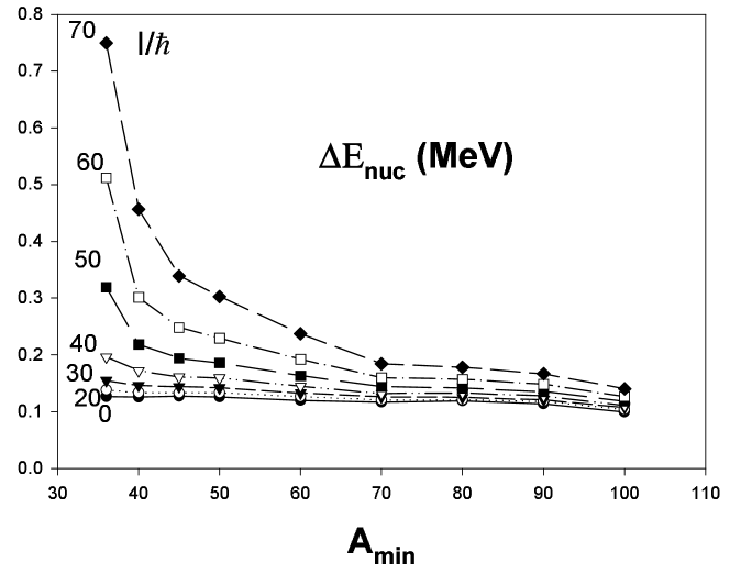
Figure 4: Root mean square energy deviation $\Delta E_{nuc}$ (in MeV) resulting from the fits of the strong interaction part of the nuclear energy at various values of the angular momentum $I$, as a function of the number of nuclei $A_{min}$ defined in the text.

The resulting energy deviations are plotted on figure 4. As a result, it appears that for angular momenta which are not too high (lower than 30-40 $\hbar$) and for intermediate values of $A_{\min}$ (in the 60-80 range) the quality of the fit seems rather stable. For large values of $A_{\min}$ the size of the data basis is probably too limited. On the other hand light nuclei at finite angular momenta $I$ seem to be not adequately represented by a liquid drop formula (as seen on Fig. 4). This is more and more so upon increasing $I$.

Table 3: Number of nuclei considered in the fit for a given lower bound $A_{\min}$ of the total nucleon number $N_{\mathrm{nucl}}$.

$A_{\min}$	34	40	50	60	70	80	90	100	110
$N_{\mathrm{nucl}}$	212	209	204	197	181	177	170	157	146

As another test of the consistency of our data basis and of its physical limitations, we have studied the convergence of the fitted LDM parameters $a_{v}$ and $a_{s}$ (Fig. 5) as well as $k_{v}$ and $k_{s}$ (Fig. 6) in terms of the number of considered nuclei $N_{\beta}$ varying as described below. We define an approximate valley of stability as a function $N(Z)$. The minimal distance of each considered nuclei to this valley is then computed. Increasing $N_{\beta}$ corresponds to including into the fit nuclei which are more and more distant from the stability curve.

The results displayed on Fig. 5 clearly demonstrate that the data basis size is just barely adequate for rough estimates of the dependence of the $a_{v}$ and $a_{s}$ coefficients as functions of $I$ at least for moderate spin values ($I<30$-40 $\hbar$). As seen on Fig. 6, at the present stage, the number of retained nuclei does not allow to draw safe quantitative conclusions on the $I$-dependence of the asymmetry coefficients $k_{v}$ and $k_{s}$.

The results obtained on Fig. 5 are consistent with a quadratic dependence of the $a_{v}$ and $a_{s}$ parameters as

$$a_{v}(I)=a_{v}(0)\left(1+c_{v}I^{2}\right)$$ (33)

and

$$a_{s}(I)=a_{s}(0)\left(1+c_{s}I^{2}\right).$$ (34)

The results of the fit of $c_{v}$ and $c_{s}$, upon using all $a_{v}(I)$ and $a_{s}(I)$ calculated for $I$ going from 0 to 40$\hbar$ by 2 $\hbar$-steps, are plotted on Fig. 7 as functions of the number of considered nuclei $N_{\beta}$ (defined as above described). These parameters are not converged, yet up to about 10 percent one may assign to them the following “asymptotic” values

$$c_{v}\approx 2.0\;10^{-5}\qquad\text{and}\qquad c_{s}\approx 1.1\;10^{-4}.$$ (35)

Let us now discuss the variation with angular momentum of the Coulomb energies. We present in Fig. 8 the evolution of the root mean square radius of the proton density as a function of the angular momentum for the four already considered nuclei. Due to the effect of centrifugal forces, it is expected that the radius should increase with an increasing angular momentum which is indeed the case here. As a consequence of their inverse proton radius dependence, the Coulomb energies (both direct and exchange terms) plotted in Fig. 9 exhibit decreasing patterns in absolute values as functions of $I$.

We have then performed a fit of the direct Coulomb energy $E_{\mathrm{CD}}$ using the two-parameter formula of Eq. (18). Since the Coulomb energy is a decreasing function of $I$, one may have expected also to observe a decreasing value of the parameter $c$ corresponding to the leading contribution to $E_{\mathrm{CD}}$. As shown on Fig. 10 this does not turn out to be the case. This incoherence is, in our opinion, due to the inadequacy of Eq. (18) to describe consistently the isospin dependence of the Coulomb energy. As described in Ref. [35], the 2-parameters formula of Eq. (18) provides a very poor fit of $E_{\mathrm{CD}}$. Indeed it yields at zero spin for the same data basis (i.e. including nuclei up to the drip-lines) a RMS energy deviation of some MeV, which is close or above the maximum of the expected spin-dependence of $E_{\mathrm{CD}}$. This is why we have performed the fit with the 5-parameters formula of Eq. (19). With this new parameterization, we obtain a parameter $c$ that now decreases with increasing $I$ (as shown on Fig. 11 together with the variation of the other fitted parameters).

As for the fit of the exchange term $E_{\mathrm{CE}}$, we obtain as demonstrated on Fig. 12 a $c^{\prime}$ parameter which decreases as a function of the angular momentum. This behavior is consistent with the above described variation of the proton radius.

The variations with $I$ of the parameters of both the strong interaction and the Coulomb part of the liquid drop model energy entail some important consequences on the nuclear deformability and hence on collective excitations as well as on the fission stability. To illustrate the latter point we have evaluated the fissility parameter $x$ defined as usual by

$$x=\frac{E_{\mathrm{Coul}}^{0}}{2E_{s}^{0}}$$ (36)

(where $E_{\mathrm{Coul}}^{0}$ and $E_{s}^{0}$ stand for the Coulomb and surface energies at zero deformation) of the $\@@nuc{236}{U}$ nucleus for spin values varying from 0 to 40 $\hbar$. In doing so, we took the surface energy as well as Coulomb direct (5 parameters fit) and exchange energies resulting from our fit. It is to be noted that even though the variation with $I$ of the parameters $k_{s}$ is not very well known quantitatively, the corrective character of the asymmetry term with respect to the total surface energy ($\sim 10$ percent) allows us to draw anyway significant conclusions on the variation of $x$ with $I$. As shown on Fig. 13, the fissility parameter decreases by $\sim 2.5$ percent when increasing the angular momentum from 0 to 40 $\hbar$. According to the liquid drop estimate for the fission barrier height $B_{f}$ of Ref. [43]

$$B_{f}\simeq 0.83\;E_{s}^{0}\;(1-x)^{3}\qquad\qquad\text{(for $x>2/3$)}$$ (37)

One sees that such a variation of $x$ corresponds to an increase of $B_{f}$ by approximately 30 percent for the considered $\@@nuc{236}{U}$ nucleus. This result, far from being insignificant, should be put into the perspective of the rotating liquid drop approach of Ref. [1]. Upon increasing the angular momentum, the rotational energy induces as well known an increased instability against fission. The variation of the fissility parameter with the spin which we have demonstrated here reduces the effective amount of the resulting fission instability.

5 Summary and conclusions

In this work, we have attempted to estimate the angular momentum dependence of the liquid drop model parameters and hence the validity of so-called rotating liquid drop model approaches making use, as well known, of a spin-independent liquid drop energy beyond the usual rotational energy term. To do so, we have first performed for 212 different nuclei at 41 different angular momentum values, state of the art self-consistent semi-classical calculations. Their results correspond to the $\hbar\rightarrow 0$ solutions (beyond the trivial Thomas-Fermi approach) of a time-reversal breaking Routhian problem using the full Skyrme SkM^∗ effective force. A particular attention has been devoted to the numerical stability of the corresponding variational solutions. The obtained strong interaction and Coulomb energies have been separately fitted into liquid drop model expressions at each angular momentum value. As a result, we have shown that our theoretical data basis was just barely capable of providing rough estimates of the angular momentum variations of the standard volume ($a_{v}$) and surface ($a_{s}$) parameters while providing only qualitative insights into the behavior of the asymmetry parameters ($k_{v}$ and $k_{s}$). The combined variation of the surface and Coulomb energies reflects itself into a sizeable variation of the fissility parameter which yields, as a consequence, an important enhancement of the fission stability for very heavy nuclei, thus partially balancing the well-known instability generated by the centrifugal forces.

Clearly, one possible continuation of the present work should consist in considerably enlarging the theoretical data basis in such a way as to extend the level of confidence in the numerical estimates of the resulting $c_{v}$ and $c_{s}$ parameters assessing the variations according to the angular momentum of $a_{v}$ and $a_{s}$. Another goal should be to have also access to the $I$-dependence of $k_{v}$ and $k_{s}$. The interest of such a numerical study could be balanced by the fact that as soon as one is only interested in the behavior of a few nuclei, one could as well perform “exact” self-consistent semi-classical calculations. However it could be argued that such calculations would necessitate, when performed for very deformed nuclei, or pieces of nuclear matter exhibiting crevices or not simply connected, etc., highly non trivial generalizations of the model densities in use for the variational problem. At any rate, it remains that our present study clearly points out the necessity to go beyond the use of a zero angular momentum parameter set when dealing with a rotating liquid drop model approach.

Some other lines of further work could be mentioned. One would consist in evaluating carefully and systematically the combined influence of the rotational energy term and of the spin-dependent liquid drop energy term on fission properties. The other set of fascinating questions stems from the negative result obtained here when trying to identify an anisotropy effect in the spatial matter distribution. It is indeed not clear to us that such a negative result should survive whenever one would deal with strongly deformed solutions. Moreover, the semi-classical solutions in use here within the scheme proposed by Grammaticos and Voros [20, 21], result from an angular averaging in the momentum space. Studying the anisotropy in this momentum space might come out at large angular velocities as another source, and may be the main source, of discrepancy between the naive spin-independent liquid drop model approach and a fully self-consistent microscopic approach of pieces of nuclear matter experiencing fast collective rotations.

Figure 1: Variation with the angular momentum $I$ of three density parameters ($\rho_{0}$, $\sigma$, $\gamma$) defined in the text, for the neutron distributions corresponding to four nuclei ($\@@nuc{90}{Zr}$, $\@@nuc{150}{Sm}$, $\@@nuc{208}{Pb}$, $\@@nuc{240}{Pu}$). The parameters $\sigma$ and $\rho_{0}$ are expressed in fm and fm^-3 respectively.

Figure 2: Same as Fig. 1 for the proton distributions.

Figure 3: Variation with the angular momentum $I$ of the neutron ($R_{n}$) and proton $(R_{p}$) sharp density radius parameters (expressed in fm) corresponding to four nuclei ($\@@nuc{90}{Zr}$, $\@@nuc{150}{Sm}$, $\@@nuc{208}{Pb}$, $\@@nuc{240}{Pu}$).

Figure 5: Fitted values of the usual volume ($a_{v}$) and surface ($a_{s}$) energy coefficients expressed in MeV, as functions of the number of nuclei $N_{\beta}$ defined in the text for various values of the angular momentum $I$.

Figure 6: Same as Fig. 5 for the usual volume ($k_{v}$) and surface ($k_{s}$) asymmetry energy coefficients.

Figure 7: Coefficients $c_{v}$ and $c_{s}$ defining the angular momentum dependence of the usual volume ($a_{v}$) and surface ($a_{s}$) energy coefficients as functions of the number of nuclei $N_{\beta}$ defined in the text.

Figure 8: Root mean square radii of the proton distributions of four nuclei ($\@@nuc{90}{Zr}$, $\@@nuc{150}{Sm}$, $\@@nuc{208}{Pb}$, $\@@nuc{240}{Pu}$) expressed in fm as functions of the angular momentum $I$.

Figure 9: Direct (“dir”) and exchange (“exc”) Coulomb energies of four nuclei ($\@@nuc{90}{Zr}$, $\@@nuc{150}{Sm}$, $\@@nuc{208}{Pb}$, $\@@nuc{240}{Pu}$) as functions of the angular momentum $I$. The l.h.s. (r.h.s. resp.) scale corresponds to the direct (exchange resp.) energies expressed in MeV.

Figure 10: Dependence of the results of the 2-parameters fit of the direct part of the liquid drop Coulomb energy in terms of the angular momentum $I$. Both parameters $c$ and $\gamma$, defined in the text, are expressed in MeV.

Figure 11: same as Fig. 10 for the 5-parameters fit.

Figure 12: Dependence of the fitted value of the parameter $c^{\prime}$, expressed in MeV, of the liquid drop exchange part of the Coulomb energy defined in the text, as a function of the angular momentum $I$.

Figure 13: Usual fissility parameter $x$ of the $\@@nuc{236}{U}$ nucleus as a function of the angular momentum $I$.

References

- [1] S. Cohen, F. Plasil and W. J. Swiatecki, Ann. Phys. (NY) 82 (1974) 557.
- [2] K. Nergaard, V. V. Pashkevich and S. Frauendorf, Nucl. Phys. A262 (1976) 61.
- [3] G. A. Anderson, S. E. Larsson, G. Leander, P. Möller, S. G. Nilsson, I. Ragnarsson, S. Āberg, R. Bengtsson, J. Dudek, B. Nerlo-Pomorska, K. Pomorski and Z. Szymanski, Nucl. Phys. A268 (1976) 205.
- [4] T. R. Werner and J. Dudek, At. Data Nucl. Data Tables 50 (1992) 179.
- [5] V. M. Strutinsky, Nucl. Phys. A95 (1967) 420 ; A122 (1968) 1.
- [6] B. Banerjee, H. J. Mang and P. Ring,Nucl. Phys. A215 (1973) 366.
- [7] A.L . Goodman, Nucl. Phys. A256 (1976) 113.
- [8] K. H. Passler and U. Mosel, Nucl. Phys. A257 (1976) 242.
-
[9]
P. Bonche, H. Flocard and P.-H. Heenen, Nucl. Phys. A467
(1987) 115;
B. Gall, P. Bonche, J. Dobaczewski, H. Flocard and P.-H. Heenen, Z. Phys. A348 (1994) 183. - [10] J. Dobaczewski and J. Dudek, Phys. Rev. C52 (1995) 1827
-
[11]
D. Samsoen, P. Quentin and J. Bartel, Nucl. Phys. A 652 (1999)
34;
D. Samsoen, P.Quentin and I. N. Mikhaïlov, Phys. Rev. C, in print. - [12] J. L. Egido and L. M. Robledo, Phys. Rev. Lett. 70 (1993) 2876.
- [13] M. Girod, J.-P. Delaroche, J.-F. Berger and J. Libert, Phys. Lett. B325 (1994) 1.
- [14] J. Bartel, P. Quentin, M. Brack, C. Guet and H.-B. Haakansson, Nucl. Phys. A386 (1982) 79.
- [15] E. Chabanat, P. Bonche, P. Haensel, J. Meyer and R. Schaeffer, Nucl. Phys. A627 (1997) 710; A635 (1998) 231.
- [16] J.-F. Berger, M. Girod and D. Gogny, Comp. Phys. Comm. 63 (1991) 365.
- [17] E. P. Wigner, Phys. Rev. 40 (1932) 749.
- [18] R. K. Bhaduri and C. K. Ross, Phys. Rev. Lett. 27 (1971) 606.
- [19] M. Brack, C. Guet and H.-B. Håkansson, Phys. Rep. 123 (1985) 275.
- [20] B. Grammaticos and A. Voros, Ann. Phys. (NY) 129 (1980) 153.
- [21] B. Grammaticos and A. Voros, Ann. Phys. (NY) 123 (1979) 359.
- [22] K. Bencheikh, P. Quentin and J. Bartel, Nucl. Phys. A571 (1994) 518.
- [23] E. Chabanat, J. Meyer, K. Bencheikh, P. Quentin and J. Bartel, Phys. Lett. B325 (1994) 13.
- [24] W. D. Myers and W. J. Swiatecki, Ann. of Phys. 55 (1969) 395 ; 84 (1974) 186.
- [25] D. Vautherin and D. M. Brink, Phys. Rev. C5 (1972) 626.
- [26] J. Dabrowski, Phys. Lett. 59B (1975) 132.
- [27] R. Bengtsson and P. Schuck, Phys. Lett. 89B (1980) 321.
- [28] K. Taruishi and P. Schuck, Z. Phys. A342 (1992) 397.
- [29] H. J Krappe, J. R. Nix and A. J. Sierk, Phys Rev. C20 (1979) 992.
- [30] A. J. Sierk, Phys. Rev. C33 (1986) 2039.
- [31] M. G. Mustapha, P. A. Baisden and H. Chandra, Phys. Rev. C25 (1982) 2524.
- [32] P. Gombas, Ann. Phys. (Leipzig) 10 (1952) 253.
- [33] H. A Bethe and R. F. Bacher, Rev. Mod. Phys. 8 (1936) 82.
- [34] C. Titin-Schnaider and P. Quentin, Phys. Lett. 49B (1974) 397.
- [35] D. Samsoen, K. Bencheikh and P. Quentin, in preparation.
- [36] P. Quentin, D. Samsoen, K. Bencheikh, E. Chabanat, J. Meyer and J. Bartel, in “Nuclear Shapes and Nuclear Structure at low Excitation Energies”, eds. M. Vergnes, D. Goutte, P.-H. Heenen and J. Sauvage, (Frontières, Paris, 1994) pp. 283-294
- [37] W. D. Myers and W. J. Swiatecki, Nucl. Phys. A81 (1966) 1.
- [38] M. Beiner, H. Flocard, Nguyen Van Giai and P. Quentin Nucl.Phys. A238 (1975) 29.
- [39] D. Vautherin, Phys.Rev. C 7 (1973) 296.
- [40] W. A. Press, S. Teukolsky, W. T. Vetterling and B. P. Flannery, Numerical Recipes in Fortran (The Art of Scientific Computing), Second Edition (Cambridge University Press, Cambridge, 1992), Chapter 10.
- [41] L. Aleksandrov, D. Karadjov and M. Drenska, Program REGN (RSIC code package PSR-165, 1981).
- [42] W. A. Press, S. Teukolsky, W. T. Vetterling and B. P. Flannery, Numerical Recipes in Fortran (The Art of Scientific Computing), Second Edition (Cambridge University Press, Cambridge, 1992), Chapter 15.
- [43] S. Cohen and W. J. Swiatecki, Ann. Phys. (NY) 22 (1963) 406.