Testing the Space-Time Structure of Event Generators
In memory of Klaus Kinder-GeigerU. Heinza,b and U.A. WiedemanncaTheoretical Physics Division, CERN, CH-1211 Geneva 23
bInstitut für Theoretische Physik, Universität Regensburg,
D-93040 Regensburg
cPhysics Department, Columbia University, New York, NY 10027
Abstract
We report on work done in collaboration with Klaus Kinder-Geiger
and John Ellis which aims at connecting the space-time structure
of event generator simulations with observable output.
Combined presentation of the talks given by the two authors at the
workshop
“RHIC Physics and Beyond – Kay Kay Gee Day”
Brookhaven National Laboratory, 23 October 1998
Klaus Geiger was an important driving force in our search for
understanding the dynamics of ultrarelativistic heavy-ion
collisions and quark-gluon plasma. An unconventional and unique
character – this is how we will remember him. Physics was his
passion, but he also loved his Porsche and his MG (=“Ma Geiger”).
It is hard for us to accept that by his untimely death
Klaus, whose research was dedicated so much to the future,
in particular to the RHIC program at Brookhaven, should be
imprisoned forever in the past. As his friends and collaborators,
we will try to carry on his legacy.
I Introduction
The main focus of Klaus’ work during the last years of his life
was the event generator VNI which describes relativistic
heavy-ion collisions and high energy particle collisions in terms
of a perturbative parton shower Monte Carlo in phase-space combined
with a simple space-time hadronization prescription. A partonic
starting point is certainly required at ultrarelativistic collision
energies, GeV, where perturbative contributions
start to account for a significant part of the measured particle
production. With his Parton Cascade Model PCM , later amended
by a space-time hadronization algorithm EG95 and made publicly
available in form of the event generator VNI VNI , Klaus Geiger
led the way.
From summer 1997 until Klaus’ death we collaborated with him and John
Ellis on implementing an afterburner for Bose-Einstein correlations into
this code and testing it in simulations for collisions at LEP I
and LEP II collisions. Our goal was to prepare for an experimental test
of the space-time dynamics predicted by VNI and to provide theoretical
guidance for multi-dimensional Bose-Einstein analyses of various event
classes with hadronic final states generated at LEP. This work
WEHG98 ; GEHW98 was interrupted prematurely; our contribution
gives an account of the present status.
VNI distinguishes itself from many other high energy event Monte Carlos
by following the event history in phase-space, not only in momentum
space. Space-time aspects enter in the numerical simulation in
various ways: On the microscopic level, the rescattering between
produced partons or hadrons is controlled by geometric cross sections,
and hadronization is modelled geometrically by requiring partons to
get (in their pair rest frame) closer than 0.8 fm in coordinate space
in order to form a hadronic cluster. On a macroscopic level
this leads to a strong density dependence of particle production and
absorption rates, further affected by the collective expansion of the
system which is generated by the rescattering. Finally, quantum
statistical effects among the produced final state particles, in
particular Bose-Einstein correlations in momentum space between pairs
of identical pions or kaons, depend on the phase-space density of
the system at the point of decoupling and thus on both the
momentum-space and space-time structure of the event at “freeze-out”
(i.e. at the point of the last strong interaction between the particles).
In this sense all measured quantities in a heavy-ion collision depend
to some extent on the space-time structure of the reaction zone. The
crucial question is, however, whether they are sufficiently sensitive
to such aspects to allow for a reconstruction of the space-time
geometry and dynamics. The successful reproduction of single-particle
yields and spectra by event generators with different space-time
features, or none at all like the popular JETSET LS95 and
PYTHIA PYTHIA generators, seems to argue against such a
possibility. Two-particle correlations in momentum space, however,
are sensitive to both the geometric extension of the “fireball” at
freeze-out and to its collective expansion dynamics WH99 .
The latter affects the two-particle spectra via so-called
“--correlations” in the emission function . This
function is the quantum mechanical analogue of the single-particle
phase-space density of the source at freeze-out: collective expansion
correlates the average direction and magnitude of the momenta of the emitted
particles with their emission points. A detailed analysis of 2-pion and
2-kaon correlations in relativistic heavy-ion collisions at the Brookhaven
AGS and the CERN SPS has recently led to an unambiguous demonstration of
strong collective dynamics of the fireballs created in these experiments
HJ99 . On a finer level, however, there remain a number of
open physical questions whose resolution requires two-particle correlation
data of similar quality and detail from elementary particle collisions.
Such data do not exist, and another motivation for our work with Klaus
Geiger was therefore to provide stimulation for similar experimental
analyses of high-statistics high energy data samples like the
million hadronic decays collected at LEP I.
For sufficiently high secondary particle multiplicities (i.e. at very
high energies or for large collision systems) it is reasonable to assume
that the two particles of a selected pair were emitted independently.
This allows to express the two-particle correlation function in terms
of the single-particle Wigner density of the source WH99 .
Neglecting final state interactions (assuming that they can be corrected
for experimentally WH99 ; HJ99 or theoretically AHR97 at a
later stage), it is given by WH99
(1)
Here are the on-shell momenta of the two particles in the pair
while and are their average and relative
4-momenta. The numerator in the second term stands for the product
of the measured single-particle spectra
(2)
where . The normalization will
be discussed below.
If, for a given momentum , the space-time dependence of can
be characterized with reasonable accuracy by a single set of rms widths
(i.e. the particle emission is not characterized by several widely
differing length scales), one can approximate by a Gaussian in
. The correlation function then takes the simple form WH99
(3)
where describes the
second space-time moments (rms widths or “homogeneity lengths”) of
the effective source of particles with momentum . Since the
two measured particles are on-shell, ,
and only 3 of the 4 components of are independent. Different
choices for the independent components lead to different Gaussian
parametrizations of the correlation function WH99 . We will here
use the Cartesian parametrization which eliminates
where is
(approximately) the velocity of the particle pair. tensysevensyfivesy is
decomposed into its Cartesian components where
denotes the “longitudinal” direction (in heavy-ion collisions this
is the direction of the beam axis, in collisions the direction
of the thrust axis), denotes the outward direction, fixed by the
azimuthal orientation of the transverse pair momentum
around the -axis, and denotes the third Cartesian (sideward)
direction (defined by , ).
Eliminating from the exponent in (3) leaves a sum over 6
terms; using furthermore the azimuthal symmetry of the event sample
around the -axis allows to further reduce this to 4 terms involving
certain algebraic sums WH99 of the rms widths
. So far, however,
Bose-Einstein correlations in elementary particle collisions
have been parametrized by much simpler Gaussian forms, involving only
one or at most two (-independent!) size parameters. Such incomplete
parametrizations have the fundamental disadvantage that the fit
parameter(s) mix(es) the interesting space-time information contained
in the rms widths of
the effective source of particles with momentum in such a way that
they can no longer be recovered He96 . An important goal of our
work with Klaus was to make predictions for the multidimensional shape
of the correlation function , by calculating the complete
set of size parameters and their -dependence.
The latter is particularly interesting since it signals
--correlations in the emission function . While in
heavy-ion collisions the dominant mechanism for such correlations
appears to be collective expansion of the fireball He96 ; WH99 ; HJ99 ,
contaminations from resonance decays after freeze-out resonances
and from --correlations in the primary hadron formation process
BZ99 (e.g. from string fragmentation) are known to exist. The
latter are expected to play a much bigger role in elementary particle
collisions where a multidimensional analysis of Bose-Einstein
correlations may help to isolate them. This would provide crucial input
into a quantitative discussion of Bose-Einstein correlations from
heavy-ion collisions where, contrary to elementary particle collisions
where the multiplicities are much lower, most resonance decays can
not be reconstructed experimentally and their effects must
therefore be simulated.
II From phase-space densities to momentum correlations
Event generators like VNI evolve classical probabilities, not
quantum mechanical amplitudes calculated from properly symmetrized
many-particle wave functions. The Bose-Einstein correlations among
pairs of identical pions or kaons must thus be included
a posteriori. For notational convenience, we restrict the
following discussion to a single particle species, say like-sign
pions. Let us assume that we have generated collision
events, and let the th event () consist
of such pions in the final state, emitted as free particles
from the phase-space points . For events,
the event generator thus simulates a classical phase-space distribution
(4)
What is needed to calculate two-particle Bose-Einstein correlations
according to (1) is a prescription which relates this classical
phase-space density with the quantum mechanical single-particle Wigner
density of the pion source which is supposed to be Monte Carlo
simulated by the event generator. In sections II.2 and II.1,
we focus on two different interpretations of the event generator output
which we call “classical” and “quantum”, respectively, although these
names should not distract from the fact that conceptually both are on an
equal footing. Each one of them leads to a different algorithm for
calculating the two-particle correlation function from the event
generator output:
(5)
Before discussing them we list three requirements which any such
algorithm should fulfill:
1.
Since the event generator evolves classical probabilities,
not symmetrized production amplitudes, the generated momenta
, do not show the enhanced
probability at low relative momenta
characteristic for Bose-Einstein final state symmetrization. The
prescriptions (5) should calculate this effect a
posteriori.
2.
The strength of Bose-Einstein correlations depends on the
distance of the identical particles in phase-space, not
in momentum space. We thus require the prescriptions
(5) to use the entire phase-space information,
and not only the generated momentum information. ‘Weighting’
or ‘shifting’ prescriptions which are based only on the
latter LS95 may successfully match the measured
momentum correlations but obviously do not allow to test the
simulated space-time structure.
3.
In general, Bose-Einstein statistics can affect particle
multiplicity distributions during the particle production
process but classical event generators do not include such
effects explicitly. Nevertheless they are tuned to reproduce
the measured average particle multiplicities .
In order not to destroy this tuning we require that the
prescription (5) conserves the single-particle
multiplicities. If the event generator were also tuned to reproduce
the average multiplicity of identical particle pairs,
, i.e. to reproduce not only the mean, but
also the width of the multiplicity distribution, then the
prescription (5) should not change that either. Interpreting
the correlator as a factor which relates the measured two-particle
differential cross section to the one simulated by the
event generator, ,
this then implies WEHG98 ; LS95 ; W98 that in
(1). The algorithms discussed below do not satisfy this
last requirement, i.e. in general they change the width of the
multiplicity distribution. However, since the space-time analysis of
correlation data can be based entirely on the momentum dependence of
, irrespective of its absolute normalization, this
does not matter for our purposes.
II.1 “Classical” interpretation of event generator output
In the “classical” interpretation ZWSH97 ; GEHW98 ,
the phase-space points
are seen as a discrete approximation of the on-shell Wigner
phase-space density :
(6)
This defines both the two-particle correlator via (1) and the
one-particle spectrum via (2). For a numerical implementation
one must replace the momentum-space -functions in (4)
by normalized “bin functions” with finite width of
rectangular ZWSH97 or Gaussian GEHW98 shape, e.g.
(7)
which reduce to the original -function in the limit
. The one-particle spectrum and two-particle correlator
then read ZWSH97 ; GEHW98
(8)
(9)
The correlator (9) is the discretized version of the Fourier
integral in (1). The subtracted terms in the numerator and
denominator remove discretization errors which would amount to pairs
constructed from the same particles. This “classical” algorithm, as well
as the “quantum” version discussed below, is numerically efficient
since it involves only manipulations per event. The
calculated observables, while being discrete functions of the input,
are continuous functions of the measured momenta, i.e. no binning
in is necessary.
II.2 “Quantum” interpretation of event generator output
The “quantum” interpretation ZWSH97 ; Weal97 ; W98 ; GEHW98 of
the event generator output starts from the observation that, for a given
event, i.e. a single term in the sum of (4), the simultaneous
sharp definition of the particle momenta and positions at emission
violates the uncertainty relation. In the limit
the sum is still expected to be a smooth phase-space function and, to
the extent that the event generator provides an accurate simulation
of the underlying QCD quantum dynamics, it is also expected to respect
the uncertainty constraints on any allowed Wigner density. Since in
practice, however, one has to work with finite numbers of events, one
may wish to ensure consistency with the uncertainty principle on the
single-event level.
This is achieved Weal97 ; ZWSH97 ; MP97 by associating the centers
of single-particle wave packets with the set of generated phase-space
points :
(10)
The describe quantum mechanically best-localized states, i.e.
they saturate the Heisenberg uncertainty relation with
and .
Taking only two-particle symmetrized contributions into account
(“pair approximation” W98 ), all spectra can be written
ZWSH97 ; Weal97 in terms of the single-particle spectrum
corresponding to an individual wave packet at phase-space
point :
(11)
(12)
(13)
Again, the subtracted terms in the numerator and denominator of
are finite multiplicity corrections which become
negligible for large particle multiplicities Weal97 .
This algorithm is consistent with an emission function
which is obtained by folding the classical distribution
of wave packet centers with the
Wigner density of a single wave packet:
(14)
(15)
The latter saturates the uncertainty relation with a spatial uncertainty
and a momentum uncertainty , and the folding ensures
that now is always quantum mechanically consistent. However,
in this algorithm both the one- and two-particle spectra depend on the
wave packet width . The role of this parameter will be discussed
in the context of our toy model study in section III.
The “classical” and “quantum” algorithms differ only with respect to
two points:
1.
The “classical” algorithm has no analogue for the
Gaussian prefactor
in (12) which is a genuine quantum effect stemming from
the quantum mechanical localization properties of (10).
2.
The Gaussian single-particle distributions in
the “quantum” algorithm are the quantum analogues of the
“bin functions” in the “classical” agorithm. With the Gaussian
bin functions (7) the two agree for the choice
. Finite event statistics puts a lower
practical limit on in the “classical” algorithm, but
to get accurate spectra one should try to choose as
small as possible, by simulating sufficiently many events. In
contrast, in the “quantum” algorithm is the finite
spatial width of the single-particle wave packets, and the limit
(which corresponds to ) is not
physically relevant: according to (14) it amounts to an
emission function with infinite spatial extension and thus
to a correlator Weal97
.
III The Zajc Model
Before describing realistic event generator simulations we
discuss some analytical results for a classical toy model
distribution . These are then used to test
the algorithms of sections II.2 and II.1,
by applying those to sets of phase-space points
generated from the model distribution with a Monte Carlo procedure.
In this way we can make quantitative statements about i) the
-dependence of the “quantum” algorithm, ii) the
-dependence of the “classical” algorithm (especially: how small
has to be chosen to extract the limit
numerically) and iii) the statistical requirements for the algorithms
to work.
The toy model, first introduced by Zajc Z93 , reads:
(16)
(17)
The distribution is normalized to a total event multiplicity .
The parameter smoothly interpolates between completely
position-momentum correlated and uncorrelated sources.
For , the position-momentum correlation vanishes
and we are left with the product of two Gaussians in tensysevensyfivesy and
tensysevensyfivesy. In the limit
(18)
the position-momentum correlation is perfect. The total phase-space
volume of the distribution vanishes
for . This strong -dependence allows to study the performance
of our numerical algorithms for different phase space volumes. In the
following subsections, we discuss the -dependence of the one-particle
spectrum and two-particle correlator, focussing in sections III.1
and III.2 on analytical results, and comparing these in
section III.3 to numerical calculations.
We recover the physical HBT radius from (21) in the limit
or by inserting (6) directly into (1).
The remarkable fact is that for sufficiently large Z93 ,
(22)
the HBT radius becomes negative and the two-particle
correlator shows an unphysical rise of the correlation function with
increasing . The change of sign in (20) seems to be
related to the violation of the uncertainty relation by the emission
function for large when tensysevensyfivesy and tensysevensyfivesy become strongly correlated.
At the critical value the phase-space volume
of the source drops below 1. Only for the
distribution is a quantum mechanically
allowed emission function, i.e. a Wigner density.
The practical importance of the Zajc model in the unphysical limit
is that it provides an extreme testing ground for
our numerical algorithms. Analytically, we conclude already from
(21) that in order to be close to the physical limit
the bin width has to be small on the scale of the
width of the generated momentum distribution,
(23)
In the above toy model this requirement is independent of the strength
of position-momentum correlations in the source.
III.2 The Zajc model in the “quantum” algorithm
Inserting the model distribution
into (14) (instead of (6)), we find
(24)
(25)
(26)
(27)
In this case, and satisfy independent of
the value of and, in contrast to the “classical” algorithm,
the radius parameter is now always positive, irrespective
of the value of . Even if the classical distribution
is sharply localized in phase-space, its folding with minimum uncertainty
wave packets leads to a quantum mechanically allowed emission function
and to a correlator with falls off with increasing
as expected. However, the spread of the one-particle
momentum spectrum (24) receives an additional contribution
. Choosing too small increases this term beyond the
phenomenologically reasonable values, choosing it too large widens
the corresponding HBT radius parameters significantly. It was
argued Weal97 that can be interpreted as quantum
mechanical “size” of the particle, fm. Given
the heuristic nature of these arguments and the significant
modifications this implies for the spectra (24) and
(25), it is however fair to say that presently
mainly plays the role of a regulator of unwanted violations of the
quantum mechanical uncertainty principle while a deeper understanding
of its origin in the particle production dynamics is still missing.
III.3 Numerical simulations in the Zajc model
We have studied the performance of our Bose-Einstein algorithms
by generating with a random number generator sets
of phase-space points according to the distribution
and comparing the numerical results
of our algorithms to the analytical expressions of section III.1
and III.2.
Figure 1:
Generic properties of the one-dimensional Zajc model. (a): HBT-radius
parameter (21) of the “classical” interpretation as a function
of the position-momentum correlation . The plot shows the
HBT radius for different combinations of the model parameters
and , and for different sizes of the bin width
used in the numerical implementation. (b): Same as (a) for
the “quantum” version (26) of the model. The dependence
of the HBT radius on the wave packet width is clearly seen.
(c) and (d): The two-particle correlator in the “classical” (c) and
“quantum” (d) version of the model for different sets
of model parameters. The numerical results are obtained for
events of multiplicity , and agree very well with the analytical
calculations.
Fig. 1(a) shows the -dependence of the HBT radius
parameter (21). For fixed bin width ,
the approximation of the true HBT radius parameter by
is seen to become better with
increasing , in agreement with (23).
For the HBT radius obtained from the “quantum” version of the
Zajc model and depicted in Fig. 1(b), the situation is
both qualitatively and quantitatively different. Now, the
HBT radius is always positive, since
the Gaussian wave packets take quantum mechanical localization
properties automatically into account. Also, the -dependence
of the radius is seen to be much weaker since the wave packets
smear out the unphysically strong position-momentum correlations
present in the classical distribution .
The HBT radius depends not only on the geometrical size , and
on the momentum width of the source, but also on the wave packet
width . As seen in Fig. 1(b), this wave packet
width affects the HBT radius and its -dependence significantly
for .
In Figs. 1(c,d) we present the two-particle
correlation functions corresponding to these HBT radius parameters
for characteristic values of the model parameters. The analytical
results, obtained by plotting (20) and (25), are
compared to the results from the event generator algorithms (12)
and (9). The plot was obtained using events of multiplicity
. The differences between analytical and numerical results
originate from statistical fluctuations and become smaller with
increasing number of events or event multiplicity .
The good agreement between analytical and numerical results in
Figs. 1(c,d) indicates the relatively low statistical
requirements of our algorithms. The reason is that both algorithms
associate with the discrete set of generated momenta
continuous functions of the measured momenta , .
This smoothens any statistical fluctuation significantly.
For the “classical” algorithm, small deviations between numerical
and analytical results are still visible in Fig. 1(c),
while the results of the “quantum” algorithm coincide
within line width. This can be traced back to the Gaussian
prefactor in (12)
which provides an additional smoothening of statistical fluctuations
not present in the “classical” algorithm.
IV Two-Particle Correlations from VNI
We have applied the “quantum” algorithm discussed above to
simulated collisions at LEP I LEP1 and LEP II LEP2
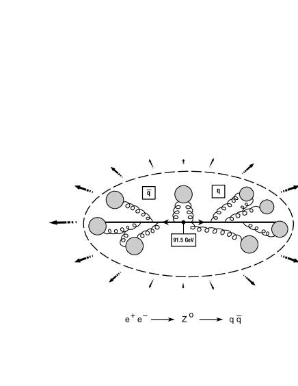
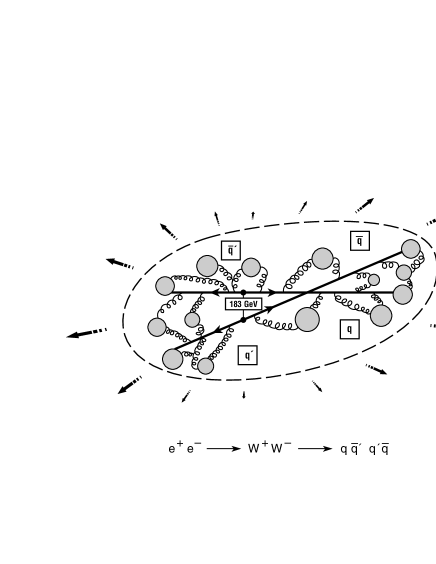
energies from VNI. We have focussed on the channels (see Fig. 2)
(28)
(29)
Figure 2:
Schematics of the two event types (28) and (29):
The final-state hadron distribution in events (left) is due to
exclusively ‘endogamous’ hadronization of the partonic offspring from
the dijet, whereas in events (right) there is, in
addition, the possibility of ‘exogamous’ hadron production involving a
mating of partons from the two different and
dijets.
which provide the “cleanest” environment for the study of
Bose-Einstein correlations in high-energy particle collisions.
Especially for the first channel there exists an impressively
extensive and accurate data sample of several million events.
For high-energy collisions, theoretical studies of Bose-Einstein
enhancements have mainly been performed within the context of the
string models strings , which have been quite successful in
reproducing the distributions of identical particle pairs on the level
of 1-parameter Gaussian fits of the correlator BEtheory .
Our study GEHW98 is based on the event generator VNI and aimed
at a full inclusion of the space-time structure of the events and
a multidimensional correlation analysis.
The “classical” and “quantum” interpretation of the event
generator output discussed in section II.1 and II.2
provide two different prescriptions for the calculation of
two-particle correlations. This ambiguity in the calculational
scheme can be traced back to the fact that both algorithms
are a posteriori remedies for an incomplete quantum
mechanical time evolution which does not account properly for
the quantum mechanical symmetrization of identical -particle
states. The ambiguity has to be removed
by a physical consistency requirement. From our discussion of
the Zajc model in section III, first crude statements about
such consistency requirements can be made:
1.
The “quantum” interpretation introduces a wave packet width
which must be adjusted to data. The measured HBT radius parameters provide
an upper bound on , . Hence, the
“quantum” interpretation can only be consistent with
experimental data if the wave packet width is not too large.
2.
In order for the “classical” interpretation of the event generator
output to be consistent with experimental data, the generated output
must not be peaked too strongly in phase-space. Otherwise, the
HBT radius may be unphysically small or even show the wrong sign,
cf. section III.1.
The first step in a realistic study of two-particle correlations
is necessarily to refine these crude statements. To what extent do
physical observables depend on the choice of algorithm? Which choice
of is consistent with experiment? Are there phenomenological
reasons to prefer one of the algorithms? These workshop proceedings
reflect the state of our work when Klaus left us. At the time of the
airline accident we had only completed the calculation with the
“quantum” algorithm, and only for a single value of the wave packet
width . A comparison of the two algorithms remains to be done.
IV.1 Two-particle correlations at vanishing pair momentum
Fig. 3 shows the correlator for different
tensysevensyfivesy-values and vanishing pair momentum tensysevensyfivesy in the c.m. frame of
the collision, . The widths of the
correlator in three Cartesian directions are roughly
the same. Quantitatively, they are roughly given by the inverse of
the wave packet width which suggests that they are dominated
Figure 3:
The correlation function of same-sign pions for different values of
the relative pair momentum tensysevensyfivesy for vanishing pair momentum tensysevensyfivesy,
.
by the “quantum mechanical smearing” features of the “quantum”
Bose-Einstein algorithm used here. A simulation with the “classical”
algorithm remains to be done.
One also sees that near the correlation functions show
characteristic deviations from a Gaussian shape. However, at non-zero
values of the orthogonal tensysevensyfivesy-components, the correlators become
nicely Gaussian. The non-Gaussian features at small tensysevensyfivesy can be traced
to decay contributions from long-lived resonances: Fig. 4
shows the same correlator
Figure 4: The correlator for
with (solid lines) and without (dashed lines) the contributions of
pions stemming from long-lived resonances.
with and without such contributions. Neglecting the pions from
long-lived resonance decays, the correlation function becomes Gaussian
and wider, reflecting a smaller source size. With long-lived resonances
included, the effective pion source is larger, resulting in
a narrower and non-Gaussian correlation function. This clearly
demonstrates the sensitivity of the correlation function on the
space-time geometry of the source function .
IV.2 Pair momentum dependence of the correlation function
As discussed before, the dependence of the correlation function
on the pair momentum tensysevensyfivesy indicates --correlations in the source
and can thus be sensitive to the space-time dynamics of hadron
production. Fig. 5 shows the correlation function
of same-sign pions for various values of the pair
momentum . Clearly, as tensysevensyfivesy increases, the
correlation function becomes wider, indicating a smaller effective
source, qualitatively (although not quantitatively) very similar to the
corresponding observations in heavy-ion collisions. This is an
interesting prediction which to our knowledge has not yet been tested
in the LEP experiments. According to the more detailed analysis
presented in GEHW98 the observed tensysevensyfivesy-dependence can be fully
attributed to the tensysevensyfivesy-dependence of resonance decay contributions;
however, this may be to some extent an artifact of the employed
“quantum” Bose-Einstein algorithm whose wave packet width
apparently dominates the widths of the correlation functions shown above.
V Outlook
The rather abrupt ending of the above section on physics results
gives a sad feeling for the gap left by Klaus. In our collaboration,
he was the only one who actually knew how to run VNI. Our original
Figure 5:
The correlation function of same-sign pions for various
values of the pair momentum , where
is the direction along the thrust axis and is the momentum transverse to it. The correlators
are plotted against one component of the relative momentum, setting the
two other components to zero.
motivation came from relativistic heavy-ion collisions where the
space-time geometry and dynamics of the event plays a crucial role
in understanding basic measurable quantities. Mainly for this reason
we developed algorithms which allow to calculate identical
two-particle correlation functions from an arbitrary event generator
output. We tested the accuracy and statistical requirements of these
algorithms in simple toy model studies and applied them in a first
realistic study to the hadronic channels in
annihilation at the -peak and near the - threshold.
However, a comparative study of both algorithms is still missing and our
main goal, the application of these algorithms to the study of
event simulations of heavy ion collisions, is not achieved yet. We
plan to do so in the near future. Also, we plan to make the algorithms
described in section II publicly available, using the
Open Standard for Codes and Routines (OSCAR) format, advocated
in YP97 .
References
(1)
Geiger, K., and Müller, B., Nucl. Phys. B 369, 600 (1992);
Geiger, K., Phys. Rev. D 47, 133 (1993);
Phys. Rep.258, 237 (1995).
(2)
Ellis, J., and Geiger, K., Nucl. Phys. A 590, 609c (1995); and
Phys. Rev. D 52, 1500 (1995).
(3)
Geiger, K., Comput. Phys. Commun.104, 70 (1997).
(4)
Wiedemann, U.A., Ellis, J., Heinz, U., and Geiger, K., in
CRIS’98: Measuring the size of things in the Universe: HBT
interferometry and heavy ion physics, (S. Costa et al., eds.),
World Scientific, Singapore, 1999.
(5)
Geiger, K., Ellis, J., Heinz, U., and Wiedemann, U.A., hep-ph/9811270,
submitted to Phys. Rev. D.
(6)
Lönnblad, L., and Sjöstrand, T., Phys. Lett. B 351,
293 (1995); Eur. Phys. J. C 2, 165 (1998).
(7)
Sjöstrand, T., Comput. Phys. Commun.39, 347 (1986);
Sjöstrand, T., and Bengtsson, M., Comput. Phys. Commun.43, 367 (1987).
(8)
Wiedemann, U.A., and Heinz, U., nucl-th/9901094, Phys. Rep., in
press.
(9)
Heinz, U., Jacak, B.V., nucl-th/9902020, Ann. Rev. Nucl. Part. Sci.49 (1999), in press.
(10)
Anchishkin, D.V., Heinz, U., and Renk, P., Phys. Rev. C 57,
1428 (1998); Sinyukov, Yu., et al., Phys. Lett. B 432,
248 (1998).
(11)
Heinz, U., in Correlations and Clustering Phenomena in Subatomic
Physics (M.N. Harakeh, O. Scholten, and J.H. Koch, eds.), NATO ASI
Series B 359, 137 (1996) (Plenum, New York).
(12)
Schlei, B.R., Ornik, U., Plümer, M., and Weiner, R.M.,
Phys. Lett. B 293, 275 (1992); Bolz, J., et al.,
Phys. Lett. B 300, 404 (1993); and Phys. Rev.
D 47, 3860 (1993); Wiedemann, U.A., and Heinz, U.,
Phys. Rev. C 56, R610 and 3265 (1997).
(13)
Bialas, A., Zalewski, K., Acta Phys. Pol. B 30, 359 (1999).
(14)
Wiedemann, U.A., Phys. Rev. C 57, 3324 (1998).
(15)
Wiedemann, U.A. et al., Phys. Rev. C 56, R614 (1997).
(16)
Zhang, Q.H., Wiedemann, U.A., Slotta, C., and Heinz, U.,
Phys. Lett. B 407, 33 (1997).
(17)
Merlitz, H., and Pelte, D., Z. Phys. A 357, 175 (1997).
(18)
Zajc, W.A., in Particle Production in Highly Excited Matter
(H.H. Gutbrod and J. Rafelski, eds.), NATO ASI Series B 303, 435
(1993) (Plenum, New York).
(19)
Hebbeker, T., Phys. Rep.217, 69 (1992);
Bethke, S., and Pilcher, J.E., Ann. Rev. Nucl. Part. Sci.42, 251 (1992).
(20)
Ballestrero, A., et al., J. Phys. G 24, 365 (1998).
(21)
Andersson, B., Gustafson, G., Ingelman, G., and Sjöstrand, T.,
Phys. Rep.97, 33 (1983);
Andersson, B., Gustafson, G., and Söderberg, B.,
Nucl. Phys. B 264, 29 (1986).
(22)
Bowler, M.G., Z. Phys. C 29, 617 (1985);
Andersson, B., and Hoffmann, W., Phys. Lett. B 169, 364 (1986);
Andersson, B., and Ringner, M., Phys. Lett. B 421, 283 (1998);
Häkkinen, J., and Ringner, M., Eur. Phys. J. C 5, 275 (1998).