Real-Time Evolution of Soft Gluon Field Dynamics in Ultra-Relativistic Heavy-Ion Collisions

Abstract

The dynamics of gluons and quarks in a relativistic nuclear collision are described, within the framework of a classical mean-field transport theory, by the coupled equations for the Yang-Mills field and a collection of colored point particles. The particles are used to represent color source effects of the valence quarks in the colliding nuclei. The possibilities of this approach are studied to describe the real time evolution of small $x$ modes in the classical effective theory in a non-perturbative coherent manner. The time evolution of the color fields is explored in a numerical simulation of the collision of two Lorentz-boosted clouds of color charged particles on a long three-dimensional gauge lattice. We report results on soft gluon scattering and coherent gluon radiation obtained in SU(2) gauge symmetry.

I Introduction

Experiments with relativistic heavy ions at center-of-mass energies reaching 100 GeV/u will soon search for a new phase of nuclear matter [1, 2]. It was argued that the extraordinarily high energy and particle number densities reached in central nuclear collisions at RHIC [3] could lead to rapid local thermalization of matter [4] and thus to the formation of the so-called quark gluon plasma [5].

One of the theoretical challenges in this context is the development of a description on the basis of quantum chromodynamics (QCD) of the processes that may lead to the formation of the locally equilibrated quark gluon plasma state in these nuclear reactions. Predictions on whether and how this state could be formed in a nuclear collision depend in a sensitive way on the initial conditions. At present, our understanding of these conditions is rather poor. Perturbative parton-parton scattering precedes local thermo-dynamical equilibrium in the early stage and may partly determine the dynamics of thermalization. Indeed, event generators based on individual parton-parton processes [6] have been developed. However, their predictions differ widely. To improve our understanding of the early stage, we have to consider the fact that the initial state is described by coherent parton wave functions and glue fields. Consequently, coherent multiple scattering must play a role in the early stage of a collision. The simplest approach to this picture would be to start with a mean field description of the color fields in an effective theory while hard modes are described through classical particles representing partons.

The possibility of a description of inelastic gluon processes by means of the nonlinear interactions of classical color fields has been proposed some time ago [7, 8]. Some years ago, this scenario was examined in studies of the collision of two transverse polarized Yang-Mills field wave packets on a one-dimensional gauge lattice [9]. These calculations showed that the interaction between localized classical gauge fields can lead to the excitation of long wavelength modes in a way that is reminiscent of the formation of a dense gluon plasma. Recently, a similar study has been carried out for collisions of Yang-Mills wave packets on a three-dimensional gauge lattice [10].

Here, we go a step further and add color charged particles to the system acting as sources of the color fields. Instead of two wave packets, we collide two clouds of such particles which shall describe the color charge distributions generated by the valence quarks in two colliding nuclei. The wave packets are now replaced by the colliding gluon fields which are generated by classical color sources while they propagate through the lattice, representing the fast moving nuclear valence quarks. The inclusion of particles also permits a comparison with perturbative calculations of gluon radiation from colliding quarks [11, 12].

We address the question whether indications for the formation of a quark gluon plasma can also be observed in such simulations. For simplicity, we leave out the hard collisions between the particles and focus first only - except from the time dependence of the color sources - on the soft dynamics in the gluon fields which are described on the lattice and correspond to modes with a small light cone momentum fraction $x$. We further leave out the hard modes of the gluon fields which may also be represented by particles. The particles may in principle be used in the future to include the semi-hard dynamics at larger $x$ following the idea of the parton cascade model [13]. While this “probabilistic” approach provides a reasonable description of large transverse momentum processes at large $x$, QCD coherence effects become important as we go to small $x$ or alternatively, towards central rapidities [14]. What is needed therefore to describe the collision of the “wee” partons is a wave picture where coherent multiple scattering is fully taken into account.

At the limit of extremely high collision energies, the model presented here has in principle to converge against a random light-cone source model which was initially proposed by McLerran and Venugopalan [15] and later further developed by these authors in collaboration with Ayala, Jalilian-Marian, Kovner, Leonidov, and Weigert [16, 17, 18, 19]. This model may therefore be used as a reference in the limit ${v/c}\rightarrow 1$. The McLerran-Venugopalan model considers very large nuclei moving with nearly the speed of light which consequently appear in the laboratory frame as “pancakes” of almost zero thickness in the transverse plane. The classical gluon field at small $x$ for a nucleus in the infinite momentum frame is obtained by solving the Yang-Mills equations in the presence of a static source of color charge on the light cone. In our approach, the solution of the equations of motion requires one to take the longitudinal extension of the nucleus into account, i.e. one must not take the nucleus to be infinitely thin in the longitudinal direction as assumed in [15]. Following Kovchegov and Rischke [20], we therefore take the finite longitudinal extension of the nuclei into account. This of course requires that the velocities of the nuclei are slightly less than the speed of light.

A major goal of the description, presented in this paper, is to keep the possibility open for an inclusion of parton cascades in the further development while the coherent physics of the random light-cone source model at small $x$ is described at the same time. This goal can only be accomplished in several steps. The approach presented here contains no restriction to central rapidities and provides therefore an extension to larger x taking into account semi-hard gluons.

In section 2, we present a brief description of the model and the formulation on a SU(2) gauge lattice. In section 3, we discuss the preparation of the initial state of the nuclei and show numerical results. In section 4, we evolve the collision and present results for the time evolution of the glue fields in the collision. A summary and conclusion is given in the section 5.

II Description of the Model

A set of equations describing the evolution of the phase space distribution of quarks and gluons in the presence of a mean color field, but in the absence of collisions, was proposed by Heinz [21, 22]. This non-Abelian generalization of the Vlasov equation can be considered as the continuum version of the dynamics of an ensemble of classical point particles endowed with color charge and interacting with a mean color field. Denoting the space-time positions, momenta, and color charges of the particles by $x_{i}^{\mu}$, $p_{i}^{\mu}$ and $q_{i}^{a}$, respectively, where $i=1,\ldots,N$ is the particle index, the equations [23] for this dynamical system read:

$$m{{dx_{i}^{\mu}}\over{d\tau}} = p_{i}^{\mu}$$ (1)

$$m{{dp_{i}^{\mu}}\over{d\tau}} = gq_{i}^{a}F^{\mu\nu}_{a}p_{i,\nu}$$ (2)

$$m{{dq_{i}^{a}}\over{d\tau}} = -gf^{abc}q_{i}^{b}p_{i}^{\mu}A_{\mu}^{c}.$$ (3)

The moving particles generate a color current ${\cal J^{\mu}}=J^{\mu}_{a}\tau^{a}/2$ which forms the source term of the inhomogeneous Yang-Mills equations

$$\bigl{[}{\cal D}_{\mu},{\cal F}^{\mu\nu}(x)\bigr{]} = g\,{\cal J}^{\nu}(x)$$ (4)

$$= g\,\sum_{i}{\cal Q}_{i}(t){{p_{i}^{\nu}}\over{m}}\delta(\vec{x}-\vec{x}_{i}(t)),$$ (5)

for the mean color field. These equations have recently been used in the weak-coupling limit ($g\ll 1$) to simulate the effects of hard thermal loops [24] on the dynamics of soft modes of a non-Abelian gauge field at finite temperature [25, 26].

Here we use Eq. (1–4) to describe the interactions among the soft glue field components of two colliding heavy nuclei. Transverse modes are included by using a 3-dimensional spatial gauge lattice. The short-distance lattice cut-off $a$ separates the regime in transverse momentum where the dynamics of gluons is perturbative (large $k_{\rm T}$) from that where perturbation theory fails (small $k_{\rm T}$) and which is of interest to us here. The interaction with the mean color field allows for an exchange of an arbitrary number of soft gluons. In combination with a parton cascade, the screening of the soft components of the gauge field by perturbative partons [27, 28] is taken into account naturally by the nonlinear nature of the coupled Eq. (1–4). This will be discussed in a separate publication [29].

We represent the valence quarks of the two colliding nuclei as point particles moving in the space-time continuum, and interacting with a classical gauge field defined on a spatial lattice in continuous time. Here we neglect the collision integrals describing hard interactions between the particles. In the spirit of the statistical nature of the transport theory, we split each quark into a number $n_{q}$ of test particles, each of which carries the fraction $q_{0}=Q_{0}/n_{q}$ of the quark color charge $Q_{0}=\sqrt{3/4}$. For the gauge group SU(2) adopted here, each nucleon is represented by two quarks, initially carrying opposite color charge. A lattice version of the continuum equations (1–4) is constructed [25] by expressing the field amplitudes as elements of the corresponding Lie algebra, i.e. ${\cal A}_{\mu},{\cal F}_{\mu\nu},{\cal E}_{k},{\cal B}_{k}\,\in$ LSU(2). As in the Kogut-Susskind model of lattice gauge theory [35] we choose the temporal gauge ${\cal A}_{0}=0$ and define the following variables.

$${\cal U}_{x,l} = \exp(-iga_{l}{\cal A}_{l}(x))\,\,=\,\,{\cal U}^{\dagger}_{x+l,-l}$$ (6)

$${\cal U}_{x,kl} = {\cal U}_{x,k}\,{\cal U}_{x+k,l}\,{\cal U}_{x+k+l,-k}\,{\cal U}_{x+l,-l}$$ (7)

Consequently, we have

$${\cal E}_{x,j} = {{-i}\over{ga_{j}}}\,\dot{\cal U}_{x,j}{\cal U}^{\dagger}_{x,j},$$ (8)

$${\cal B}_{x,j} = {{i\,\epsilon_{jkl}}\over{4ga_{k}a_{l}}}\,\bigl{(}{\cal U}_{x,kl}-{\cal U}^{\dagger}_{x,kl}\bigr{)},$$ (9)

for the electric and magnetic fields, respectively. The lattice constant in the spatial direction $j$ is denoted by $a_{j}$. As one can see from (6), the gauge field is expressed in terms of the link variables ${\cal U}_{x,l}\,\epsilon$ SU(2), which represent the parallel transport of a field amplitude from a site $x$ to a neighboring site $(x+l)$ in the direction $l$. We choose ${\cal U}_{x,k}$ and ${\cal E}_{x,k}$ as the basic dynamic field variables and solve the following equations of motion for the fields.

$$\dot{\cal U}_{x,k}(t) = i\,g\,a_{k}\,{\cal E}_{x,k}(t)\,{\cal U}_{x,k}(t)\qquad\qquad\qquad\qquad\qquad$$ (10)

$$\dot{\cal E}_{x,k}(t) = {i\over{2ga_{1}a_{2}a_{3}}}\sum\limits^{3}_{l=1}\Bigl{\{}{\cal U}_{x,kl}(t)-{\cal U}^{\dagger}_{x,kl}(t)\,\Bigr{.}$$ (11)

$$- \,\Bigl{.}{\cal U}^{\dagger}_{x-l,l}(t)\,\Bigl{(}{\cal U}_{x-l,kl}(t)-{\cal U}^{\dagger}_{x-l,kl}(t)\Bigr{)}\,{\cal U}_{x-l,l}(t)\,\Bigr{\}}$$ (12)

$$- \,g\,{\cal J}_{x,k}(t).$$ (13)

In the time evolution of the particle lattice system, these equations have to be solved simultaneously together with the equations (1) to (3). The dynamics of the particles is described within a dual lattice which is defined by the edges of the Wigner-Seitz cells of the original lattice. The charge of all particles in the volume of one cell is associated with the center of the cell represented by a point of the real lattice. As long as a particle propagates in the cell its charge vector is not changed. If a particle crosses the boundary of a dual box, the charge is transported parallel to the center of the neighbor cell into which the particle enters. Exchange of energy between a particle and the field occurs only at the transition from one dual box into another. The particle is reflected from the wall if its kinetic energy is smaller or equal than the work required to move the charge from the old box into the new box. In the other case, a transition into the new box occurs where the amount of energy required to make the transition is either subtracted or added to the kinetic energy of the particle depending on the sign of the product $Tr({\cal Q}_{i}{\cal E}_{x,l})$. This mechanism provides a coupling between the fields and the particles which allows to generate color fields through color charge currents. The method has the advantage that it exactly preserves the law of Gauss. It also preserves the conservation of energy which is thus only violated through numerical errors of the order $\Delta t^{3}$ in the time integration of the field equations (10) and (11). On the other hand, the method, as simple as it is, is connected with serious limitations as for example the violation of causality when the time step width $\Delta t$ is smaller than the lattice constants $a_{l}$. $\Delta t$ can not be chosen larger than $a_{l}$ because the time integration of the equations (10) and (11) is instable for $\Delta t\geq{\rm min}(a_{l}:l=1,2,3)$ These limitations do not yet allow a study of the dynamics of the particles in a microscopically correct way. Artifacts, as for example a trapping of particles of too small kinetic energy in dual cells can occur. For propagating nuclei, the field energy associated with a single link can occasionally exceed the kinetic energy of a particle resulting in the emission of particles due to backwards scattering from the link. This corresponds to the (unphysical) emission of nucleons from the moving nuclei, which we want to avoid.

However, a slight modification of the above described procedure for the wall transition of particles allows to use the particles to simulate color charge fluctuations and to generate coherent color fields: We leave the kinetic energy of a particle unchanged whenever it crosses a cell boundary of the dual lattice and only transport its color charge to the neighboring lattice cell. This is equivalent to setting the Coulomb force in the r.h.s. term of Eq. (3) to zero. In this way, the collection of particles acts as a classical color source propagating through the lattice with constant velocity.

III The Initial State

In the following, we briefly outline how, in principle, a simulation of a nuclear collision is performed within the model described in the previous section. Mainly, however, we discuss the question how to generate the “initial state”.

For a central collision of two Pb nuclei one would expect that 34 nucleons in a row collide on the collision axis (z-axis). This number is desired from the following estimate. We denote the nucleon radius by $r_{n}$, the proton radius of a nucleus by $R_{P}$ and the neutron radius of a nucleus by $R_{N}$. The average number of nucleons in a cylinder of the radius $r_{n}$ around the collision axis is determined by

$$n=n_{P}+n_{N}={3\over 2}\Bigl{(}\Bigl{(}{{r_{n}}\over{R_{P}}}\Bigr{)}^{2}Z+\Bigl{(}{{r_{n}}\over{R_{N}}}\Bigr{)}^{2}N\Bigr{)}.$$ (14)

With the values $r_{n}=1.32\,{\rm fm}$, $R_{P}=5.47\,{\rm fm}$, $R_{N}=5.80\,{\rm fm}$ from Ref. [30], we find the result $n=17.11$ for ${}^{208}Pb$.

In accordance with the spatial extension of a nucleon we choose a lattice extension of 1.2 fm into both transverse directions. The lattice spacing is taken $a_{l}=0.3$ fm in each direction, thus $4^{2}\times 40$ lattice points cover the volume of 17 nucleons in one row. More correctly, since there is no Pauli-Principle between neutrons and protons there are two superposed rows of nucleons. One row contains 8 protons and the other 9 neutrons. These details, however, are far beyond the reach of our calculation, and we simply take 16 nucleons or 32 quarks (in SU(2)) in our initial state. We also use the rounded value $r_{n}=1.2$ fm. The coverage of two complete nuclei in the transverse plane requires much larger lattices and remains a challenge for more extended calculations in the future. The lattice is closed to a 3-torus which means that we apply periodic boundary conditions in all three spacial directions. The fact that we use a lattice with transverse extensions much smaller than the radius of a nucleus leads to restrictions. The first of these is that we can not simulate the full transverse dynamics of a collision. Such simulations for central collisions are possible but they require lattices with transverse extensions at least twice as large as the radius of a nucleus. Second, for lattices with small transverse extensions, the periodic boundary conditions in the transverse directions define a situation which is equivalent to the assumption that the nuclei have infinite extension into transverse directions. Therefore, in this respect, our description stays firmly within the framework of the model of McLerran and Venugopalan [31]. Larger lattice sizes will be necessary to carry out a meaningful Fourier analysis of the fields in transverse directions and to compare results of both models. However, the transverse extension of a nucleon can be covered at least to describe the initial state of nucleons.

As already mentioned above, a dual lattice is superimposed on the original lattice in such a way that the lattice points are located in the centers of the cells of the dual lattice. The dual lattice cells are used to associate particles with lattice sites and thus to define the source terms in (4). To generate the initial configurations of the nuclei, we randomly distribute color charged massless particles over the volume such that each lattice cell is occupied by an even number $n_{b}$ of particles. The total initial color charge is zero in each box corresponding to a neutral color charge distribution. Momenta with opposite but random directions and Boltzmann distributed absolute values are assigned to each pair of particles . The Momenta are renormalized such that the total initial kinetic energy of the particles in one nucleus agrees with half of the correct mass of 16 nucleons ($M=8\cdot m_{n}=8\cdot 939$ MeV) while we assume that half of the nucleon energy is carried by glue fields. This procedure fixes the temperature parameter $T$ in the Boltzmann distribution for the particles.

The initial configuration of a single nucleus in its rest frame is obtained through the evolution of the equations (1 – 3), (10), and (11) over a long period of time starting from the initial fields ${\cal E}_{x,k}(t=0)=0$, ${\cal U}_{x,k}(t=0)={\bf 1}_{2}$. The simulation of a collision requires a Lorentz boost of each nucleus into the center of velocity frame of both nuclei. In the example presented below, the kinetic energy is 100 GeV/u for which $\gamma=106.5$. Both nuclei are mapped into their initial positions on a large Lorentz-contracted lattice right after the boost of particle coordinates $x_{i},p_{i}$ and field amplitudes.

At this point, it has to be emphasized that it is not possible to boost fields on a lattice. We have extensively explored the possibility to generate the color fields before the Lorentz-boost. In this case one would generate the initial state of the nucleus before the boost by evolving the equations of motion in time until an equilibrium between kinetic particle energy and field energy is accomplished. This would require to employ the algorithm without the modification mentioned in section 2. The Lorentz-transformation of such a “initial state”, however, does not lead to a configuration which propagates stably along the lattice. One reason is that the lattice dispersion relation is not boost invariant. After the boost, the Fourier components of the fields do not match with the finite discrete Fourier spectrum of the lattice. Another reason is that the Hamiltonian of the system does not commute with the boost operator. We have found it most practical to boost the particle coordinates $x^{\mu}_{i},p^{\mu}_{i}$ at time $t=0$ for both nuclei, wherafter the fields are generated from the initial conditions ${\cal E}_{x,k}(t=0)=0$ and ${\cal U}_{x,k}(t=0)={\bf 1}_{2}$. It has been argued [1] that the coupling constant $\alpha_{s}$ should be taken at an effective momentum scale on the order of $2\pi T$ corresponding to $g=2$. Starting from $g=0$, the coupling constant is increased slowly until it reaches a final value $g=2$. This method leads to quasi-stable configurations propagating over distances which extend over several thousand lattice points in the longitudinal direction. It avoids the problem with the lattice dispersion since the discretized k-space is fixed after the boost. The adiabatic increase of the coupling constant avoids the excitation of instable high frequent modes in the color fields [32].

However, it requires large initial distances between the nuclei because the charge fluctuation $\mu$ converges slowly against a final constant value before the collision. Also, the fields should carry enough energy. For nucleons with the correct mass ($m_{n}=939$ MeV) about half of the total energy are carried by glue fields. If we want to satisfy this condition to a better approximation then also semi-hard gluons have to be taken into account. The largest fraction of these $50\%$ is carried by soft gluons with a Bjorken scale $x\leq 0.1$, followed by semi-hard gluons with $0.1<x<0.2$. In the original work of McLerran and Venugopalan [15], only the valence quarks were taken to be sources of color charge which gave $\mu^{2}\sim A^{1/3}\,{\rm fm}^{-2}$. Hence $\mu\gg\Lambda_{QCD}$ only for nuclei much larger than physical nuclei. However, if semi-hard gluons are also included as sources of color charge (as they should be) then $\mu^{2}$ is defined as [33]

$$\mu^{2}={{A^{1/3}}\over{\pi r_{0}^{2}}}\int_{x_{0}}^{1}dx\Bigl{(}{1\over{N_{c}}}q(x,Q^{2})+{{N_{c}}\over{N_{c}^{2}-1}}g(x,Q^{2})\Bigr{)}$$ (15)

where $q,g$ stand for the nucleon quark and gluon structure functions at the resolution scale of $Q$ of the physical process of interest. Using the HERA structure function data, Gyulassy and McLerran estimated that $\mu\leq 5\,{\rm fm}^{-1}$ for LHC energies and $\mu\leq 2.5\,{\rm fm}^{-1}$ at RHIC energies. Since semi-hard gluons appear at $x$ values which correspond to rapidities greater than the central rapidity in nuclear collisions, we have to describe also the longitudinal dynamics of the fields in the collision. Such a description is possible on a gauge lattice with a finite extension into the longitudinal direction as used in the subsequent calculation. For a resolution of the longitudinal dynamics, the fact that the nuclei move with a speed smaller than speed of light becomes very important. This situation is depicted in the following Fig. 1.

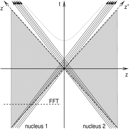
FIG. 1.: The trajectories of two colliding nuclei (thin solid lines) are displayed together with the light cone (dot dashed lines). All components of the nuclei stay in the light cone throughout the collision since they propagate slower than speed of light. Consequently, the nuclei have a finite extension in the z-direction. The dashed horizontal line indicates the direction in which we carry out the Fourier analysis of the initial state of a single nucleus.

The finite longitudinal extension of the nuclei is also necessary for the propagation of the fields on the lattice.

In the following, we demonstrate that the proposed description allows to generate an “initial state” with a finite but small charge fluctuation. For the above chosen lattice constants each nucleon is covered by 40 lattice cells of the dual lattice. Each of these boxes is initially occupied by an even number $n_{b}$ of color charged particles such that the sum over all charges in a box is zero. The initial charge density thus is zero on a length scale of the lattice spacing and larger. At the initial time $t_{0}$ both nuclei, i.e. the particles, are boosted with the same $\gamma$ but into opposite directions towards the center of collision. The lattice constants $a_{l}$ and the time step width $\Delta t$ are Lorentz transformed accordingly. The initial distance $d_{0}$ of the nuclei is chosen $16000$ lattice spacings. $d_{0}$ is Lorentz contracted to $45.07$ fm in the center of velocity frame. According to the above fixed extensions into transverse directions and size of the nuclei, we use a lattice that comprises a total of $4^{2}\times 16384$ points. We repeat the calculation for a longitudinally refined lattice which comprises a total of $4^{2}\times 32768$ points. In this case, the propagation starts at $d_{0}=32000$ lattice spacings while the longitudinal lattice spacing is reduced to $a_{3}=0.1\,{\rm fm}$, i.e. a single nucleus is then covered by $4\times 4\times 120$ lattice cells.

While the nuclei translate on the lattice, we adiabatically increase the coupling constant with a rate of $\Delta g/\Delta t\leq(3000a)^{-1}$ until $g$ has reached its final value ($g=2.0$). The propagating particles transport color charges from one box to another and the charge density becomes different from zero and shows fluctuations in coordinate space. The spacial charge density on the lattice is defined by

$$\rho^{c}_{x}(t):=\sum_{i\in I_{x}(t)}{{q_{i}^{c}(t)}\over{a_{1}a_{2}a_{3}}},$$ (16)

where $I_{x}(t)$ denotes the set of particle indices of the particles which are in the dual box of the site $x$ at time $t$. The upper index denotes the color while the lower index refers to the lattice site at which the density is evaluated. In Fig. 2, the distribution $d(t,q^{c}_{x})$ of the charge per box is displayed at several different time steps $t_{n}$. The charge with color $c$ per box at site $x$ is defined as

$$q_{x}^{c}(t):=\rho^{c}_{x}(t)a_{1}a_{2}a_{3}$$ (17)

At time $t=0$ all $q_{x}^{c}(t=0)$ are zero and $d(t,q^{c}_{x})$ is different from zero only in the bin around $q_{x}^{c}=0$. In the continuum limit $a_{l}\rightarrow 0$ this would correspond to $d(t=0,q_{x}^{c})\sim\delta(q_{x}^{c})$. From such a configuration we can generate a configuration possessing a finite charge fluctuation or a finite $\mu$ respectively.

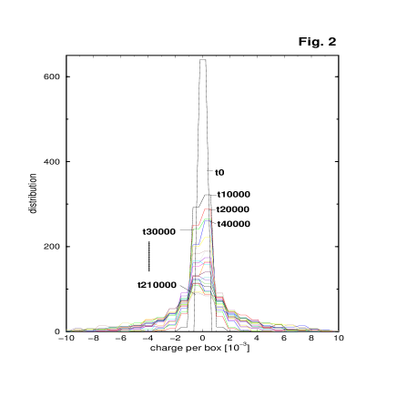
FIG. 2.: The computed distributions of the charge per box for a boosted nucleus ($\gamma=106.5$, $4\times 4\times 40$ dual lattice cells, $n_{b}=6$, $a_{1}=a_{2}=a_{3}=0.3\,{\rm fm}$) for increasing times. The time is indicated at the curves by the time step numbers $t_{n}$.

As already mentioned above, the initial positions, momenta and color charge orientations are chosen randomly. The chaotic nature of the Yang-Mills equations enhances strongly the convergence towards color distributions in position space which fluctuate in a highly statistical manner, i.e. the information about the initial distributions becomes strongly washed out after some time.

Fig. 2 shows for one color, that the distribution of the charge density increases in width monotonously with time. The corresponding width is displayed in Fig. 5. Surprisingly, the shape of the distributions seems to be different from Gaussian distributions. This difference is explained in the following way. The shape of the distributions in Fig. 2 results from a superposition of two Gaussian distributions of different widths which become equal after long times. In order to show that this effect results from the Lorentz boost, we display in Fig. 3 the color charge per box distribution of an unboosted nucleus. These distributions become Gaussian after relatively short times as indicated by the small time step numbers $t_{n}$ in the figure.

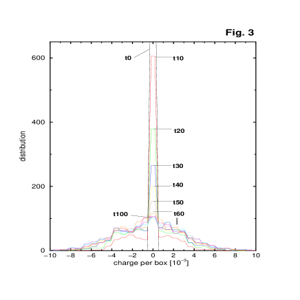
FIG. 3.: The same distributions as in Fig. 2 but for an unboosted nucleus ($10\times 10\times 10$ dual lattice cells, $n_{b}=6$, $a_{1}=a_{2}=a_{3}=0.3\,{\rm fm}$).

For a boosted nucleus, the lattice is Lorentz contracted in the longitudinal direction. The randomly generated coordinates of the particles imply a color charge fluctuation which appears after short times in the distributions. In addition to the propagation of the charges, a rotation in color space occurs at a charge when it crosses a cell boundary. These rotations lead to an additional smoother broadening of the charge distributions in each color. The rotation depends on the length of the link and the strength of the color electric field pointing in the direction of the boundary transition. On a Lorentz contracted lattice, charges that cross transverse boundaries experience a much stronger rotation than charges which cross longitudinal boundaries because the transverse links are longer and the transverse color electric fields are stronger than the longitudinal components. Indeed, for small times we find a shape of the charge distribution similar to that in Fig. 2 in the time evolution of an unboosted collection of particles on a (by arbitrary choice) deformed lattice.

The curves in Fig. 2 from $t_{10000}$ to $t_{40000}$ contain a slightly broadened high “peak” in the center and a wide part at the bottom. In order to show that the slow increase of the width of the central peak results from longitudinal color rotations we refine the lattice in the longidutinal direction by a factor three as already mentioned above while keeping the volume of the nucleus constant. The number of particles increases by a factor three while the length of the charge vector is reduced by a factor three.

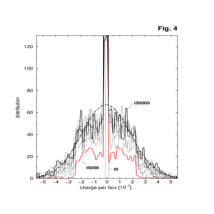
FIG. 4.: The same distributions as in Fig. 2 but for a refined lattice ($\gamma=106.5$, $4\times 4\times 120$ dual lattice cells, $n_{b}=6$, $a_{1}=a_{2}=0.3\,{\rm fm}$, $a_{3}=0.1\,{\rm fm}$). The dashed curve shows the Gaussian fit of the distribution at time step $t_{50000}$.

In Fig. 4, we display the color charge distributions for a boosted nucleus in the case of a finer longitudinal lattice. The central peak decays gradually in time but stays narrow in comparison with the wide distribution at the bottom and in comparison with the central peak in Fig. 2. The distribution displayed for the time step $t_{5000}$ results essentially from charge propagation. The width of this distribution corresponds exactly to the length $q_{0}$ of a charge vector. At later times color rotation seems to smear out the distribution. At $t_{50000}$ which is close before the collision, the distribution has a Gaussian shape. In principle one would have to evolve much longer in time until the central peak is smeared out. The time step numbers in Fig. 4 are much larger (by a factor $\gamma^{2}$) than in Fig. 3. This is explained by the fact that the boosted particles propagate essentially into the longitudinal direction. In addition, the time step width is reduced by a factor $\gamma^{-1}$.

In the subsequent calculations, we neglect the resulting final changes of the width because they are small. We find the same time behavior of the distributions for all colors. The fluctuation of the charge density $\delta\rho^{c}_{\rm Latt}$ is associated with the width of the distributions shown in the figures Fig. 2 and Fig. 4. Numerically, $\delta\rho_{\rm Latt}$ is determined by

$$(\delta\rho^{c}_{\rm Latt})^{2}:={1\over{(a_{1}a_{2}a_{3})^{2}}}\sum_{x}\bigl{(}\sum_{i\in I_{x}}q_{i}^{c}\bigr{)}^{2},$$ (18)

where we make use of the fact that

$$\sum_{x}\sum_{i\in I_{x}}q_{i}^{c}=0.$$ (19)

FIG. 5.: The fluctuation of the charge density $\delta\rho_{\rm Latt}$ on the lattice (upper solid curve) is displayed for a Lorentz contracted nucleus (see units on axis of ordinates) as a function of time over the number of time steps. The time step width is $\Delta t=0.03/\gamma\,{\rm fm}$. The dashed curve shows the same but averaged over two points.

In Fig. 5, we display $\delta\rho^{c}_{\rm Latt}$ of the distributions shown in Fig. 2 as a function of time. Fig. 5 shows, how $\delta\rho^{c}_{latt}$ evolves after the Lorentz boost when the nucleus propagates along the contracted lattice. The curves show that $\delta\rho^{c}_{\rm Latt}$ begins to converge at large times. In Fig. 6, we display $\delta\rho^{c}_{\rm Latt}$ of the distributions shown in Fig. 4 as a function of time. The curves are plotted for all colors.

We now make an estimate of the transverse average charge density $\mu$ used in the McLerran Venugopalan model [15]. The correct way to determine this quantity is rather involved since $\mu$ is related to a surface charge density in the transverse plane. The calculation of this surface charge density requires a parallel transport on the SU(2) mainfold of all charges in the longitudinal direction from the spacial site of the charge into a fixed transverse plane, e.g. the central transverse plane of a nucleus. The surface charge density which follows from that procedure leads to a distribution of charges per plaquette in the transverse plane. For reasonable statistics, the transverse extension of the lattice has to be large enough. The transverse extension of our lattice however is small and we therefore give a simple estimate. We assume that, according to translational symmetry of the unboosted three dimensional lattice, the distributions shown in Fig. 2 and Fig. 3 are equal to the distribution which we would obtain for each transverse layer of boxes from a lattice with large transverse extension. The convolution over all transverse charge density distributions leads to the surface charge density distribution in one transverse plane. Supposing that the distributions have a Gaussian shape, we determine $\mu$ by

$$\mu={1\over{N_{c}^{2}-1}}\sum_{c}\delta\rho^{c}_{latt}a_{3}\sqrt{a_{1}a_{2}{\tilde{N}_{3}}}.$$ (20)

$\tilde{N}_{3}$ denotes the number of lattice cells which cover a nucleus in the longitudinal direction and corresponds to the number of convolutions.

FIG. 6.: Same as Fig. 5 but for a lattice with $4\times 4\times 2^{15}$ points and constants $a_{1}=a_{2}=0.3\,{\rm fm}$, $a_{3}=0.1\,{\rm fm}$. A nucleus is covered by $4\times 4\times 120$ dual lattice cells.

In the calculation of the curves in Fig. 5 and Fig. 6, we have used $n_{b}=6$. According to Fig. 5 and Fig. 6, we obtain the final values $\mu=0.06\,{\rm fm}^{-1}$ and $\mu=0.04\,{\rm fm}^{-1}$. These values stay below the estimate of Gyulassy and McLerran [33]. The value of $\mu$ or $\delta\rho$ respectively is one important criterion for the construction of the initial state before the collision. Since the charge $Q_{0}=\sqrt{3/4}$ is fixed for SU(2) quarks and $g=2$ according to [1], $n_{b}$ and the transverse lattice constants $a_{1}$, $a_{2}$ are the remaining parameters which determine $\mu$.

Another important criterion is that the distribution of soft gluons and semi-hard gluons should reproduce the longitudinal momentum distribution $g(x,Q^{2})$ which is observed experimentally. To reproduce $g(x,Q^{2})$ would be far too ambitios but at least we have to consider the momentum distribution. The gluon distributions in momentum space are simply related to the Fourier transformed gauge field $A_{\nu}^{c}(\vec{k})$ by $|2{\rm Tr}({\cal A}_{\nu}(\vec{k}){\cal A}_{\nu}(\vec{k}))|$ (no summation over $\nu$. The light cone model of McLerran and collaborators describes the initial state through pure gauge fields

$$A^{\pm} = 0,$$ (21)

$$A^{i} = \Theta(z^{-})\Theta(-z^{+})\alpha_{1}^{i}(x,y)+$$ (23)

$$\Theta(z^{+})\Theta(-z^{-})\alpha_{2}^{i}(x,y)\quad i=1,2.$$

The coordinates $z^{\pm}$ are defined as $z^{\pm}={1\over{\sqrt{2}}}(t\pm z)$.

In the following, we call the direction $l=3$ which is parallel to the collision axis the “longitudinal” direction and $E,A$-field amplitudes associated with longitudinal links are called the “longitudinal fields” $E_{\rm L}$. The fields $E_{\rm T}$ in transverse directions are called “transverse”. The Fourier transformation of the field of one nucleus along the dashed line in Fig. 1 leads to a distribution of the form $|A_{i}(k_{3})|^{2}\sim{1/{k_{3}^{2}}}$. The electric field follows from the equations (21) and (23) by the definition $E=-\partial_{t}A$. The transverse electric field along the dashed line Fig. 1 has the z-dependence $E_{i}\sim\delta(z-z_{0})\,(i=1,2)$ while the longitudinal electric field $E_{z}=0$ or $E^{\pm}=0$ respectively. The Fourier spectrum of the color electric field is therefore a constant and shows no $k_{3}$-dependence. The following results presented in this section have been calculated for a single nucleus which propagates on a lattice of the size $4^{2}\times 16384$ points. In Fig. 7, we display as a function of the Fourier index $\tilde{k}_{3}=k_{3}a_{3}/(2\pi)$ at the time step $t_{80000}$, the longitudinal Fourier spectrum of the transverse gauge field which we calculate according to

$$f_{\rm T}^{(A)}(t,k_{3}):={1\over{2N_{1}N_{2}(N_{c}^{2}-1)}}\sum_{x,y}\sum_{c}\sum_{l=1,2}A^{c}_{l}(t,x,y,k_{3}).$$ (24)

The corresponding Fourier spectrum of the transverse color electric field is calculated as

$$f_{\rm T}^{(E)}(t,k_{3}):={1\over{2N_{1}N_{2}(N_{c}^{2}-1)}}\sum_{x,y}\sum_{c}\sum_{l=1,2}E^{c}_{l}(t,x,y,k_{3}).$$ (25)

at the same time step. The gauge fields $A_{l}^{c}(t,x)$ have been determined on the lattice through time integration of the color electric fields along the whole time evolution. The momentum distribution in Fig. 7 agrees (if one compares the normalized distributions) with the result obtained for $f_{\rm T}^{(E)}(t,k_{3})$. This check tells us that the gauge fields $A_{l}^{c}(t,\vec{x})$ displayed in Fig. 9 (a) are true in a sense that they really correspond to the color electric fields. In Fig. 8, the Fourier spectrum of the longitudinal gauge field is displayed on a logarithmic scale, i.e. $\log_{10}(|f_{\rm L}^{(A)}(t,k_{3})|^{2}k_{3}^{2})$ is plotted as a function of the Fourier index $\tilde{k}_{3}=k_{3}a_{3}/(2\pi)$. The figure shows that the longitudinal components of the fields carry very low longitudinal momenta in comparison to the longitudinal momenta in the transverse components. Most of the longitudinal field energy is in modes with $\tilde{k}<34$ while the transverse field energy is in modes up to $\tilde{k}=3400$.

Fig. 9 (a) shows for all colors the gauge fields generated by a nucleus which moves from the left to the right in the figure. The steep front of the field distribution indicates the position of the nucleus.

FIG. 7.: Longitudinal Fourier-spectrum of the transverse gauge fields $|f_{\rm T}^{(A)}(t_{80000},k_{3})|^{2}k_{3}^{2}$ in units of $10^{5}\,{\rm fm}^{-4}$ plotted as a function of the Fourier index $\tilde{k}_{3}$.

Lets assume that the color electric field $E_{l}^{c}(z)$ is finite and constant inside of the nucleus and zero outside of the nucleus, i.e. $E_{l}^{c}(z)=1$ for ${{-\Delta z}\over{2}}\leq z\leq{{\Delta z}\over{2}}$ and $E_{l}^{c}(z)=0$ for $z>{{\Delta z}\over{2}}$ or $z<{{-\Delta z}\over{2}}$. The Fourier transformation of such a static rectangular field distribution has the form

$$\tilde{E}_{l}^{c}(k_{3})={{2^{3/2}}\over{\pi}}{{\sin{({{\Delta z}\over 2}k_{3})}}\over{k_{3}}}$$ (26)

from which we conclude that the half period of $|E_{l}^{c}(k_{3})|^{2}$ in $k$-space is $\Delta k_{3}={{2\pi}\over{\Delta z}}$. This difference can also be expressed in terms of the Fourier index as $\Delta\tilde{k}={{N_{3}a_{3}}\over{\Delta z}}$. For a moving nucleus, the Fourier spectrum is shifted as can be seen in Fig. 7. The width of the large hump in Fig. 7 corresponds to the longitudinal extension of the boosted nucleus which is $\Delta z=40a_{3}$ while $N_{3}=16384$.

FIG. 8.: The longitudinal Fourier-spectrum of the longitudinal gauge fields is shown as a function of the Fourier index $\tilde{k}_{3}$ on the logarithimic scale as $2\log_{10}{\bigl{(}|f_{\rm L}^{(A)}(t_{8}0000,k_{3})|k_{3}\bigr{)}}$. The argument of the logarithm is given in units of ${\rm fm}^{-2}$.

In Fig. 9 (a), we display a snap shot of the gauge field amplitudes $|\overline{A}^{c}(t,z)|^{2}$ taken as average over the transverse planes at the time step $t_{100000}$. Fig. 9 (b) shows for the same time step the corresponding transverse energy density distribution which we define as

$$w_{\rm T}^{(E)}(z)=Tr({\cal E}_{1}{\cal E}_{1})+Tr({\cal E}_{2}{\cal E}_{2}).$$ (27)

Further below, we will also need the longitudinal energy density distribution which is defined

$$w_{\rm L}^{(E)}(z)=Tr({\cal E}_{3}{\cal E}_{3}).$$ (28)

The figures Fig. 9 (a) and Fig. 9 (b) clearly show that the gauge field behind the moving color sources is mostly a pure gauge field because the amplitude of the color electric field behind the nucleus is zero. Large amplitudes of the color electric field appear only inside of a nucleus which has a finite extension in the longitudinal direction. The gauge fields displayed in Fig. 9 (a) correspond to the gauge fields of the light cone model according to the ansatz in Eq. (21). In the light cone model, behind a nucleus, they are constant along lines parallel to the collision axis. These fields, however, are not unique due to gauge freedom. Therefore, the gauge fields in Fig. 9 (a) can be very different from the ansatz in Eq. (21).

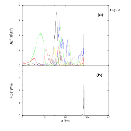
FIG. 9.: The transverse gauge fields $|\overline{A}^{c}(t_{100000},z)|^{2}$ averaged over the transverse plane and squared are displayed for each color in the upper panel. In the lower panel, we show the corresponding transverse color electric field energy density $w_{\rm T}^{(E)}(t_{100000},z)$.

IV The Collision

In the previous section, we have outlined how a collision can be simulated on a gauge lattice with small transverse extension and how the initial state can be generated within the model. In this section, we focus on the time period after the collision and discuss results obtained from simulations of a collision on two different lattices. In one case we performed a calculation on a lattice of the size $4\times 4\times 2^{15}$ points using lattice constants $a_{1}=a_{2}=0.3\,{\rm fm}$ and $a_{3}=0.1\,{\rm fm}$. Accordingly, a single nucleus is covered by $4\times 4\times 120$ dual lattice cells. In the following the refer to this paramerization as the “case (1)”. In the second case, we performed a calculation on a lattice of the size $4\times 4\times 2^{14}$ points using lattice constants $a_{l}=0.3\,{\rm fm}\,(l=1,2,3)$. A single nucleus is thus covered by $4\times 4\times 40$ lattice cells. We refer to this parametrization as the “case (2)”. A time-step width of $\Delta t=0.03/\gamma$ fm is used in both cases. In the case (2), we construct initial states as “realistic” as possible within the model. We try to ajust the glue field energy of the nucleon, to obtain a color charge fluctuation $\mu$ in the range estimated by other authors and to describe the longitudinal size of the Lorentz boosted nucleus. We expect that this calculation provides a non-perturbative estimate for soft glue field scattering and glue field radiation at high energies. Due to the high color field energies the simulation of case (2) is close to the limit of acceptable numerical precision. An improvement requires finer but also larger lattices exceeding our computational resources. Instead, we refine the lattice in case (1) keeping the size small. In this case the fields carry less energy before the collision but the resolution of the field dynamics is higher and more precise. Case (1) therefore provides a control over the qualitative nature of the results while we expect some quantitative results from case (2). Most of the figures presented below are shown for case (1). The curves agree in a qualitative manner with results obtained in case (2) but they show less intensity.

In Fig. 9 (b) of the previous section, we have shown the transverse color electric field energy density distribution $w_{\rm T}^{(E)}(z)$ of a propagating nucleus for one time step. To get a full picture of the evolution of $w_{\rm T}^{(E)}(t,z)$ and $w_{\rm L}^{(E)}(t,z)$ during the generation of the initial state when the two nuclei approach each other, we display in Fig. 10 (a) and (b) the energy densities of the transverse and longitudinal components of the $E$-field every 10000 time steps for the case (1).

FIG. 10.: The transverse (a) and longitudinal (b) energy densities of the color electric fields are displayed for two approaching nuclei. The numbers on top of the distributions indicate the number of steps in the time integration (on top of left nucleus) or time in units of fm (on top of right nucleus).

We verified, that the corresponding $B$-field energy densities $w^{(B)}(z)$ are almost identical with $w^{(E)}_{\rm T}(z)$. After 1000 time steps (not shown in the figure) the transverse $E$-field energy $W^{(E)}_{\rm T}$ is by about a factor $\gamma/2$ larger than the longitudinal $E$-field energy $W^{(E)}_{\rm L}$. This ratio increases to $\gamma$ at 50000 time steps and remains constant afterwards.

As Fig. 10 (a),(b) shows, two configurations representing two nuclei propagate remarkably stably (nucleus 1 from left to right and nucleus 2 from right to left) over long distances on the lattice. The collision begins at $t_{53333}$ where the fields of both nuclei make first contact.

In Fig. 11 at time step $t_{50000}$ of case (1), the particle density (in units of 20 on the ordinate), which is defined as the number of particles per bin of width $a/10$ in longitudinal direction, is superimposed on the transverse and longitudinal field energy densities (multiplied by a factor 10 in the figure) for comparison. The particle density defines the extension of the nucleus in the longitudinal direction. The mismatch between particle density and field energy density decreases when the density of lattice points covering the nucleus in the longitudinal direction is increased. This requires a shift of the cutoff (here at $k_{c}=2.0$ GeV for $a=0.3\,{\rm fm}$) to higher momenta.

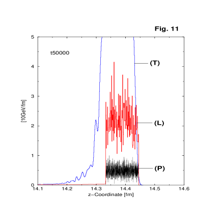
FIG. 11.: Comparison of the transverse (T) and longitudinal (L) color electric field energy distribution in a single nucleus with the distribution of the particles. The longitudinal energy density has been multiplied by a factor 10 for better comparison. The particle density (P) has been divided by a factor 20.

The tails of the field energy densities result not only from lattice dispersion effects. The lattice is Lorentz contracted in the longitudinal direction and particles have large longitudinal momentum components. Therefore, particles primarily transfer energy into longitudinal links. The nonlinearity of the Yang Mills equations provides a mechanism transferring energy from longitudinal into transverse degrees of freedom. Field amplitudes which are left behind on the longitudinal links are canceled by following particles of rotated color charge.

FIG. 12.: The transverse color electric field energy density is displayed for case (1) at various different time steps after the begin of the collision. The total time step number $t_{n}$ and the relative time $t$ counted from the first contact of the nuclei is indicated in each panel. The collision begins at the total time step $t_{53333}$ or at the relative time $t=0\,{\rm fm}$ respectively. The particle distributions (multiplied by a factor 1/10) are included in panel (a) and (b).

Fig. 12 displays snap shots of $w^{(E)}_{\rm T}(t_{n},z)$ 1667, 6667, 11667, 16667, 21667 and 26667 time steps after the begin of the collision. In the panel (a) and (b) the particle distributions in coordinate space (multiplied by a factor 1/10) are displayed together with the field energy distributions to indicate the position of the receding nuclei.

As compared to Fig. 11, the width of the distributions $w^{(E)}_{\rm T}(t,z)$ moving with the particles is considerably increased (about $30\%$). This sudden change of the width occurs during the overlap of the nuclei. At the same time the field amplitudes at the position of the particles have decreased. We would expect that this leads to an increased energy transfer from the particles into the fields. To explore this behavior, we define the electric field energy for each color

$$W_{c}^{(E)}(t)={{a_{1}a_{2}a_{3}}\over 2}\sum_{x\in X}\sum^{3}_{l=1}E^{c}_{x,l}E^{c}_{x,l}.$$ (29)

Note, that we do not sum over the color index c. The magnetic field energy $W_{\rm T}^{(B)}(t)$ is defined in the same manner. In the calculations, we find that $W_{c}^{(B)}(t)\simeq W_{c}^{(E)}(t)$. We calculate the integrated field energy $W_{c}^{(E)}(t)$ as a function of time. Fig. 12 will be further discussed below.

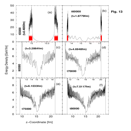
FIG. 13.: Same as in Fig. 12 but for the longitudinal color electric field energy density $w^{(E)}_{\rm L}(z)$.

In Fig. 14, we display for case (2) $W_{c}^{(E)}(t)$ for each $c$ in a time interval around the time of first contact $t_{80000}$. In the time region between $t_{80000}$ and $t_{90000}$, we observe a kink (it is a bit washed out) in $W^{(E)}_{c}(t)$, which increases remarkably in the collision (see also Fig. 15). In the upper left corner, we display for case (1) $W^{(E)}(t)=\sum_{c}W_{c}^{(E)}(t)$ in a time interval around $t_{53333}$. The angle between the dashed line and the dot-dashed line indicates the kink. The kink in Fig. 14 corresponds to an increased energy transfer from the particles into the fields while the nuclei recede. This tells us that the energy deposit between the receding nuclei results not only from the interaction between the fields during the overlap time but glue field radiation contributes. The contributions to glue field radiation appear in the longitudinal field energy density distributions shown in Fig. 13. Energy is transfered from the particles into the fields through longitudinal links. Before the collision during the generation of the initial state this transfer occurs smoothly generating coherent fields. The strong increase of $w^{(E)}_{\rm L}(t,z)$, at times larger than the time of the kink and further away from the center of collision, results from the fact that more energy is transfered into longitudinal links than the closest transverse links can absorb from them during the short time in which a nucleus passes a certain longitudinal link. The distribution $w_{\rm L}^{(E)}(z)$ increases sharply for collision times larger $0.3\,{\rm fm}$ and arrives at a first maximum at $t\simeq 0.5\,{\rm fm}$. The next minima appear at a time $t\simeq 0.7\,{\rm fm}$ which could presumably be interpreted as a thermalization time for the soft glue fields. It corresponds to the FWHM of the valley in Fig. 13 (c).

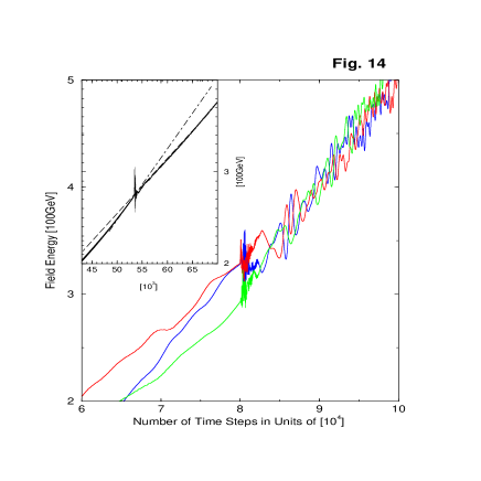
FIG. 14.: The total color electric field energy $W_{c}^{(E)}(t)$ for each color is displayed for case (2) in the time interval between $t_{60000}$ and $t_{100000}$. The panel in the upper left corner displays the total electric field enery for case (1). The lines indicate a kink.

When the two nuclei pass through each other, the particles experience the combined fields of both nuclei. The corresponding changes of the field amplitudes enter into the r.h.s. of (3) and modify the orientation of the color charge vectors $\vec{q}_{i}^{a}(t)$ during the rather short overlap time of $0.11\,{\rm fm}$. This induces net color charge currents resulting in radiation of gluons. Since the longitudinal momenta of the particles are large compared with their transverse components, color charges move essentially parallel to longitudinal links and induce electric fields on these links. Before the collision, the charge of the following particles was polarized such that these fields were canceled. After the collision this is no longer true over a long period of time. A continuation of the time evolution has shown that the longitudinal energy density of the fields remains as large as in Fig. 13 and decreases slowly at very large times.

The excess of energy remaining in the longitudinal links propagates then into transverse directions. These longitudinal fields possess only transverse momenta and result in gluon radiation into transverse directions. This mechanism describes gluon radiation from the particles. The fact that the transverse extension of our lattice is very small and periodically closed does not really allow an expansion of the radiated glue fields into transverse directions. They collide with other radiated gluons and are stopped. This feature is somewhat unphysical and can only be removed by taking lattices with large transverse extensions. The radiated glue fields remain therefore essentially on the longitudinal links and decay slowly. However, at least it allows one to determine how much is radiated from a certain volume.

We therefore define the color separated longitudinal electric field energy

$$W_{{\rm L},c}^{(E)}(t)={{a_{1}a_{2}a_{3}}\over 2}\sum_{x\in X}E^{c}_{x,3}E^{c}_{x,3},$$ (30)

which is a function of time. Fig. 15 displays $W_{{\rm L},c}^{(E)}(t)$ for all colors. The kink in the time dependent field energy of Fig. 14 appears much stronger in Fig. 15. The curves in Fig. 15 show essentially the cumulative time integral of how much energy is radiated from the particles at increasing time.

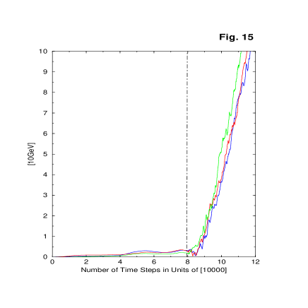
FIG. 15.: Longitudinal color electric field energy as function of time.

In the following, we discuss the contribution to the energy deposit which results from the interaction of the fields. The contribution of the particles will be discussed later. We discuss the results for two choices of the lattice size and lattice spacing. The numbers, obtained in the case where we use a $4\times 4\times 16768$ lattice are given in parentheses. As we see from Fig. 12, a considerable fraction of the transverse field energy is deposited around the center of collision between the receding nuclei.

At the time step $t_{160000}$ in the case (2), about $440\,{\rm GeV}$ of the total transverse electric field energy $W^{(E)}_{\rm T}=2810\,{\rm GeV}$ are left in the spatial region between $z_{1}=3.08\,{\rm fm}$ and $z_{2}=43.08\,{\rm fm}$ (the center of collision is at $z=23.08\,{\rm fm}$). The field energy density between the nuclei is about a factor $1/100$ smaller compared to the field energy density at the position of the particles in the receding nuclei. Due to the large space volume between $z_{1}$ and $z_{2}$ however, the energy deposit amounts to about $16\%$ of the total energy in soft field modes.

Fig. 13 shows that the longitudinal energy densities are small but finite around the center of collision. The calculation shows in case (2) that within short times $\Delta t=1.0\,{\rm fm}$ after the begin of the collision about $23\,\%$ ($7.42\,{\rm GeV}$) of the total field energy deposit ($31.98\,{\rm GeV}$) that is left in the region between $z_{1}=22.08\,{\rm fm}$ and $z_{2}=24.08\,{\rm fm}$ are carried by longitudinal components of the $E$-field. The average ratio $w^{(E)}_{\rm L}/w^{(E)}_{\rm T}$ in this region is about 0.6 which is large compared to the above mentioned factor $1/\gamma$. This ratio appears to be even larger in case (1). Within the short time $\Delta t=0.3\,{\rm fm}$ after the begin of the collision about $29\%$ ($664\,{\rm MeV}$) of the total field energy deposit ($2270\,{\rm MeV}$) left in the region between $z_{1}=15.08\,{\rm fm}$ and $z_{2}=15.68\,{\rm fm}$ are contained in longitudinal component of the $E$-field.

Since the color charge and color current density is zero, the linearized Yang-Mills equations (4) are homogeneous in this region and allow only for solutions with non-zero amplitudes into transverse directions in relation to the direction of their energy flow. Figure 10 displays the fraction with momenta pointing into transverse direction relative to the collison axis. The longitudinal field energy density in the narrow space region between $z_{1}=15.08\,{\rm fm}$ and $z_{2}=15.68\,{\rm fm}$ is not a result of gluon radiation. A calculation with the right-hand side of (2) and (3) set to zero just before the nuclei make first contact yields the same results in that narrow region, which finds its explanation in a transfer of energy from the propagating transverse fields to the longitudinal fields due to the non-linear coupling between $E_{\rm T}$ and $E_{\rm L}$ in (4). Also in collisions of Yang-Mills wave packets, where no particles are taken into account, we observed a strong increase of the longitudinal fields around the center of collision during the overlap of the wave packets [10].

When the two nuclei overlap during the collision, the fields are superposed. As a result of the nonlinear terms in (4), which act as source terms for the longitudinal fields, the amplitudes $E^{c}_{\rm L}$ start to grow rapidly during the short overlap time (of the particle clouds) of $0.11\,{\rm fm}$. This mechanism describes the scattering of soft gluons which occurs over a much longer period of time. To analyze this process within the model, we define the following quantities. The Poynting vector in the adjoint representation is denoted as

$$\vec{\cal S}:=c\,\vec{\cal E}\times{\cal B}.$$ (31)

With the transverse and longitudinal components of the vector (31) we define the total transverse and longitudinal energy currents

$$i_{T}(t):=2\sum_{l=1}^{2}\int d^{3}x\,\big{|}{\rm Tr}\bigl{(}{\cal S}_{l}(t,\vec{x})\bigr{)}\big{|}$$ (32)

$$i_{L}(t):=2\sum_{l=3}^{3}\int dx^{3}\,\big{|}{\rm Tr}\bigl{(}{\cal S}_{l}(t,\vec{x})\bigr{)}\big{|}.$$ (33)

In the following Fig. 16, we display $i_{T}(t)$ (panel (a)) and $i_{L}(t)$ (panel (b)) for the time interval between $t_{50000}$ and $t_{70000}$. Fig. 16 (a) shows that shortly after the first contact of the nuclei there is a sudden increase of the transverse energy current in the fields. This increase describes soft gluon scattering into transverse directions. The slope of the dot-dashed line indicates the current corresponding to the energy rate transfered from the particles to the fields if no collision would occur. The dot-dashed line rpresents an underground which has to be subtracted from the curve to determine the contribution that results from scattering. A very similar behavior has recently been found in collisions of color polarized wave packets on the three-dimensional lattice [10]. At the same time, Fig. 16 (b) shows that the longitudinal energy current decreases remarkably during the overlap of the fields. The width of the inverse peak in Fig. 16 (b) corresponds to a time of $0.18\,{\rm fm}$ which is the overlap time of the fields. After the overlap, the curve approaches the dot-dashed line almost as close as before the collision. This leads to the conclusion that the inverse peak is a interference phenomenon. Nevertheless, it determines the time interval in which the fields interact. The steady increase of the longitudinal current before the collision results from the energy transfer from particles into fields. In a similar study for case (2), we find that the transverse energy current keeps increasing much stronger long after the collision. These additional contributions describe glue field radiation.

FIG. 16.: The transverse (panel (a)) and longitudinal (panel (b)) energy currents $i_{T}(t)$ and $i_{L}(t)$ are displayed in a time interval around the beginning of the collision.

To give an estimate for glue field radiation, we integrate the curve in Fig. 13 (f) from $z_{1}=8.38\,{\rm fm}$ to $z_{2}=22.38\,{\rm fm}$ and find an energy deposit of $64.62\,{\rm GeV}$. This energy divided by the volume covered by both particle distributions and divided by the time of $t=7.51\,{\rm fm}$ since first contact yields a radiation power of about $115\,{\rm GeV/fm^{4}}$. In the case (2) we find the result $110\,{\rm GeV/fm^{4}}$ over a time of $23\,{\rm fm}$. We now give estimates for contributions from soft scattering and radiation. The total field energy at the time step $t_{80000}$ amounts to $757.24\,{\rm GeV}$ in case (1) while the field energy deposit in the space region between $z_{1}=8.38\,{\rm fm}$ and $z_{2}=22.38\,{\rm fm}$ is $94.74\,{\rm fm}$. We conclude that $8\%$ of the total field energy are deposited between the nuclei at $t=7.51\,{\rm fm}$. In case (2), we find $26\%$ at $t=23\,{\rm fm}$.

Finally, we analyze the momentum distribution in the transverse color electric fields. In the previous section we have discussed the Fourier spectrum of the initial state of a single nucleus. Now, we transform the fields of two nuclei propagating at the same time on a lattice of the size $4\times 4\times 2^{15}$ according to case (1). In the upper panel (a) of Fig. 17, we display the normalized longitudinal momentum distribution of two nuclei at time step $t_{50000}$ shortly before the beginning of the collision. With Eq. (25) it is defined as

$$\overline{f}_{\rm T}^{(E)}(t,k_{3}):=f_{\rm T}^{(E)}(t,k_{3})\Bigl{[}\int_{0}^{\infty}dk_{3}f_{\rm T}^{(E)}(t,k_{3})\Bigr{]}^{-1}$$ (34)

In the lower panel (b), we display the momentum distribution after the collision at the time step $t_{80000}$. A comparison of Fig. 17 (a) with Fig. 17 (b) shows evidence for the production of a final state with a momentum distribution that dramatically differs from that of the initial state.

FIG. 17.: The normalizd Fourier spectra of the transverse color electric field before (a) and after the collision (b). The snap shots are taken at the time steps $t_{n}$ indicated on top of the curves. In the upper left corner of panel (b)), we display the cumulative integrals over the spectra.

In the upper right corner of Fig. 17 (b), we display the cumulative integrals over the distributions

$$\overline{F}_{\rm T}^{(E)}(t,k_{3}):=\Bigl{[}\int_{0}^{\infty}dk_{3}f_{\rm T}^{(E)}(t,k_{3})\Bigr{]}^{-1}.\int_{0}^{k_{3}}dk^{\prime}_{3}f_{\rm T}^{(E)}(t,k^{\prime}_{3})$$ (35)

We compare the results for $t_{50000}$ (solid curve) and for $t_{80000}$ (dashed curve). Above $\tilde{k}=2200$, the dashed curve is clearly below the solid curve which shows that energy is transfered from high frequent modes into low frequent modes during the collision. This behavior has also been found in collisions of color polarized Yang-Mills wave packets in 1+1 dimensions [9] and later in collisions of Yang-Mills wave packets in 3+1 dimensions [10] and could presumably describe particle production [32]. Our calculation shows that this pure classical phenomenon occurs also in collisions of Yang-Mills fields which are not polarized in color space.

V Summary and Conclusion

In the framework of a classical effective approach of QCD, color charged particles have been employed to generate the color source effects of the valence quarks in ultra-relativistic nuclear collisions. Classical Yang-Mills fields have been used to describe soft modes of the gluons. We have studied the time-evolution of such a system of particles and fields by solving the coupled system of Wong equations and Yang-Mills equations, as a transport model for the reaction of nuclei in collisions at high energies. We have carried out numerical simulations of the collision on a long three dimensional gauge lattice with small transverse extensions. Results have been presented which demonstrate the properties of such a description from various aspects and provide estimates for contributions at small transverse momenta. We have discussed the similarities and the basic differences of the approach presented in this paper as compared to the light cone source model [14, 16, 17, 18, 19, 20]. It has been demonstrated that a “initial state” can be generated which describes the longitudinal extension, the color charge fluctuation and the glue field energy of the nuclei before the collision. The shape of the longitudinal momentum distribution of the soft gluons in the initial state as obtained in our calculation is similar to the shape of the experimentally know gluon distribution at small $x$.

As a function of time, we have calculated the transverse and longitudinal energy densities of the color electric fields. For an effective coupling of $g=2$ and for an energy of $100\,{\rm GeV/u}$, our calculation predicts that a relatively large fraction (over $8\%$) of the total soft field energy (at small $x$) contributes at $t=7.5\,{\rm fm}$ after the first contact to the energy deposit between $z_{0}\pm 7\,{\rm fm}$ around the center of collision $z_{0}$.

The colliding color fields cause soft gluon scattering. This has been demonstrated in a calculation of the transverse and the longitudinal energy current as a function of time throughout the collision.

The non-linear nature of the Yang-Mills equations causes a change of the color charge distribution in the two colliding clouds of particles during the overlap time which results in an increase of the charge fluctuation. The resulting color charge currents lead to an averaged gluon radiation from the particles which amounts to $110\,{\rm GeV/fm^{4}}$ (radiation power per particle volume) over times of $7\,{\rm fm}$ and even $20\,{\rm fm}$.

The longitudinal momentum distributions of the transverse color electric fields have been calculated. The fields were not polarized in color space. Our results show that an energy transfer from high frequenzy modes into low frequenzy modes occurs in the collision. The same observation has been made by Hu et al. [9] studying collisions of color polarized pure Yang-Mills wave packets on a one-dimensional SU(2) gauge lattice. The Fourier analysis of section 5 shows that the existence of this phenomenon does not require color polarization in the initial conditions, e.g. before the collision.

In this paper we have discussed a new approach to describe ultra-relativistic heavy-ion collisions in a coherent way in 3+1 dimensions. We have presented results from numerical model simulations to explore the possibilities for describing results from experiments. A combination of our approach with parton cascades and ultra-relativistic quantum molecular dynamics could allow to trace further back from experimental data into the early stage of the collision. The approach for itself could describe the formation of the quark gluon plasma within the classical mean field approximation.

At the present stage, we are still far from accomplishing such goals. It would be important to increase the extension of the lattice into transverse directions to cover two nuclei completely. This would allow to determine the soft transverse momentum distributions and the time evolution of single transverse modes. Also a study of the dynamics of the particles will be necessary. This requires that the particles are fully coupled to the fields. The momentum distributions and rapidity distributions of the particles could be compared with experiment.

We thank S.G. Matinyan, D.H. Rischke, and R. Venugopalan for helpful discussions. This work was supported by the U.S. Department of Energy under Grant No. DE-FG02-96ER40495.

REFERENCES

- [1] J. W. Harris and B. Müller, Annu. Rev. Nucl. Part. Sci. 46, 71 (1996).
- [2] A.V. Smilga, Phys. Rep. 291, 1 (1997).
- [3] M. Gyulassy, Nucl. Phys. A590, 431c (1995).
- [4] E. Shuryak, Phys. Rev. Lett. 68, 3270 (1992); K.J. Eskola and M. Gyulassy, Phys. Rev. C 47, 2329 (1993).
- [5] B. Müller, Rep. Prog. Phys. 58, 611 (1995).
- [6] X.N. Wang and M. Gyulassy, Phys. Rev. D 44, 3501 (1991); 45, 844 (1992); Phys. Rev. Lett. 68, 1480 (1992); Phys. Lett. B282, 466 (1992); K. Geiger and B. Müller, Nucl. Phys., B369, 600 (1992).
- [7] H. Ehtamo, J. Lindfors, and L. McLerran, Z. Phys. C18, 341 (1983).
- [8] A. Kovner, L. McLerran, and H. Weigert, Phys. Rev. D 52, 3809 and 6231 (1995).
- [9] C.R. Hu, S.G. Matinyan, B. Müller, and A. Trayanov, Phys. Rev. D 52, 2402 (1995).
- [10] W. Pöschl and B. Müller, preprint DUKE-TH-98-179, nucl-th/9812066, submitted to Phys. Rev. D (1998).
- [11] Yu. V. Kovchegov, Phys. Rev. D 54, 5463 (1996).
- [12] S.G. Matinyan, B. Müller and D. Rischke, Phys. Rev. C 57 1927 (1998).
- [13] K. Geiger, Phys. Rep. 258 237 (1995).
- [14] R. Venugopalan, Comments in Nucl. and Part. Phys. 22 113 (1998).
- [15] L. McLerran and R. Venugopalan, Phys. Rev. D49 2233 (1994); D49 3352 (1994); 50 2225 (1994).
- [16] A. Ayala, J. Jalilian-Marian, L. McLerran and R. Venugopalan, Phys. Rev. D52 2935 (1995); D53 458 (1995).
- [17] J. Jalilian-Marian, A. Kovner, L. McLerran and H. Weigert, Phys. Rev. D55 5414 (1997).
- [18] J. Jalilian-Marian, A. Kovner, A. Leonidov and H. Weigert, Nucl. Phys. B504 415 (1997).
- [19] J. Jalilian-Marian, A. Kovner, and H. Weigert, hep-ph/9709432.
- [20] Yu.V. Kovchegov and D.H. Rischke, Phys. Rev. C 56, 1084 (1997).
- [21] U. Heinz, Phys. Rev. Lett. 51, 351 (1983); Ann. Phys. (NY) 161, 48 (1985); 168, 148 (1986)
- [22] H.-Th. Elze and U. Heinz, Phys. Rep. 183, 81 (1989)
- [23] S.K. Wong, Nuovo Cim. A 65, 689 (1979)
- [24] R. Pisarski, Phys. Rev. Lett. 63, 1129 (1989); E. Braaten and R. Pisarski, Phys. Rev. D 42, 2156 (1990).
- [25] C.R. Hu and B. Müller, Phys. Lett. B409, 377 (1997)
- [26] G.D. Moore, C.R. Hu and B. Müller, Phys. Rev. D 58, 045001 (1998)
- [27] T.S. Biró, B. Müller, and X.N. Wang, Phys. Lett. B283, 171 (1992)
- [28] K.J. Eskola, B. Müller, and X.N. Wang, Phys. Lett. B374, 20 (1996)
- [29] S.A. Bass, B. Müller, and W. Pöschl, Duke University preprint DUKE-TH-98-168 (nucl-th/9808011).
- [30] Y.K. Gambhir, P. Ring, and A. Thimet, Ann. Phys. 198, 132 (1990).
- [31] A. Krasnitz and R. Venugopalan, preprint NBI-97-26, hep-ph/9706329.
- [32] C. Gong, S.G. Matinyan, B. Müller, and A. Trayanov, Phys. Rev. D 49, 607 (1994).
- [33] M. Gyulassy and L. McLerran, Phys. Rev. C56 2219 (1997).
- [34] U. Heinz, Phys. Lett. B 144, 228 (1984)
- [35] J. Kogut and L. Susskind, Phys. Rev. D 11, 395 (1975)