THREE-PION EXCHANGE:
A GAP IN THE NUCLEON-NUCLEON POTENTIAL

Abstract

The leading contribution to the three-pion exchange nucleon-nucleon potential is calculated in the framework of chiral symmetry. It has pseudoscalar and axial components and is dominated by the former, which has a range of about 1.5 fm and tends to enhance the OPEP. The strength of this force does not depend on the pion mass and hence it survives in the chiral limit.

PACS codes: 13.75.Cs, 13.75.Gx, 12.39.Fe, 11.30.Rd

Keywords: nucleon-nucleon interaction, chiral symmetry

I Introduction

The nucleon-nucleon (NN) interaction has been studied for more than 50 years, but it is still not fully understood. The research program proposed by Japanese physicists around 1950 [2] and based on the idea that the outer part of the interaction is due to mesonic exchanges proved to be very successful. Quite generally, the spatial features of a given process are determined by the mass exchanged in the $t$-channel and lighter systems correspond to longer interaction ranges. The lightest NN exchange, associated with the one-pion exchange potential (OPEP) became a consensus in the sixties, giving rise to a generation of models in which waves with $L>5$ were treated theoretically [3].

The second layer of the interaction is much more complex and was studied in the following two decades, by means of a detailed treatment of the two-pion exchange potential (TPEP) [4, 5]. This process depends on an intermediate pion-nucleon ($\pi$N) scattering amplitude and reflects strongly its dynamical content.

In the present decade, most of the research work on the NN potential was aimed at constructing the TPEP in the framework of chiral symmetry. This symmetry was developed around 1960, for systems in which pions and nucleons were considered as elementary. Nowadays one believes QCD to be the basic theory of strong interactions and, accordingly, that pions and nucleons are made of light quarks, interacting by means of gluon exchanges. As the QCD Lagrangian predicts that gluons can interact among themselves, calculations at low and intermediate energies are very difficult. The usual strategy for overcoming this problem consists in working with effective theories that treat pions and nucleons as elementary and include, as much as possible, the main features of the basic theory. The fact that the masses of the u and d quarks are close to each other and very small in the hadronic scale means that QCD is approximately invariant under the chiral group SU(2)$\times$SU(2). One therefore requires the effective theories to possess approximate chiral symmetry, besides the usual Poincaré invariance.

In low energy processes, chiral symmetry is realized in the Nambu-Goldstone mode and the vacuum is filled with a condensate, that allows the excitations of massless collective states, identified with the pions. The breaking of the symmetry, due to the quark masses at the fundamental level, is associated with the small pion masses in the effective theories.

Chiral symmetry is very important in the theoretical treatment of two-pion exchange because it constrains the intermediate $\pi$N amplitude. At low and intermediate energies it is given by a nucleon pole contribution, superimposed to a smooth background [6]. The symmetry is responsible for large cancellations within the nucleon sector that, at once, settle the scale of the problem and amplify the role of the background. The latter is very important, since the chiral nucleon sector in isolation does not suffice for explaining $\pi$N experimental data.

The construction of the TPEP in the framework of chiral dynamics motivated most of the research of this decade, beginning with the work of Ordóñez and van Kolck [7], who considered a system containing just pions and nucleons. Several works followed, dealing with complementary aspects of the problem [8, 9] and nowadays this part of the NN interaction is well understood. Predictions for NN observables produced by just the OPEP and the chiral TPEP, assumed to represent the full interaction for distances larger than 2 fm, were calculated and shown to agree well with experiment [10]. Therefore the effort based on chiral symmetry led to an important refinement of outer part of this interaction and brought theoretical constraints to waves with $L\geq 3$.

In the case of the NN interaction, it is important to note that the importance of chiral symmetry depends strongly on the process one is considering. In the case of the OPEP, for instance, it is completely irrelevant, for predictions from chiral $\pi$N Lagrangians coincide with those arising from interactions without any symmetry. All Lagrangians, symmetric and non-symmetric, produce exactly the same basic pion-nucleon vertex, showing that chiral symmetry is compatible with and, at the same time, irrelevant for the OPEP [11]. In the case of the TPEP, on the other hand, the symmetry is crucial. It produces internal cancellations in the intermediate $\pi$N amplitude which yield a potential that vanishes in the chiral limit.

To our knowledge, only contributions due to the exchanges of one and two pions have been so far studied in the framework of chiral symmetry. In order to extend this picture, here we study the component of the NN potential due to the exchange of three uncorrelated pions. This system has a mass around 450 MeV and its effects should be longer than those of the vector mesons usually present in one-boson exchange potentials. The basic interaction is closely related to the amplitude for the process $\pi$N$\rightarrow\pi\pi$N. Hence, we review briefly the main features of this reaction in sect.II and calculate the potential in sect.III.

II Pion Production

The NN interaction mediated by the exchange of three uncorrelated pions is derived from $T_{cba}$, the amplitude for the process $\pi^{a}(k)N(p)\rightarrow\pi^{b}(q)\;\pi^{c}(q^{\prime})N(p^{\prime})$. This amplitude is given by the diagrams of fig.1 and written as the sum of $T_{cba}^{\pi}$, representing the class of processes with a pion pole in the $t$-channel, and a remainder, denoted by $\bar{T}_{cba}$, whose dynamical content is indicated in fig.1. In the framework of chiral symmetry, this last amplitude is given by a basic family of diagrams, involving only pions and nucleons, supplemented by other processes, containing deltas, rhos, omega and the $\pi N$ $\sigma$-term.

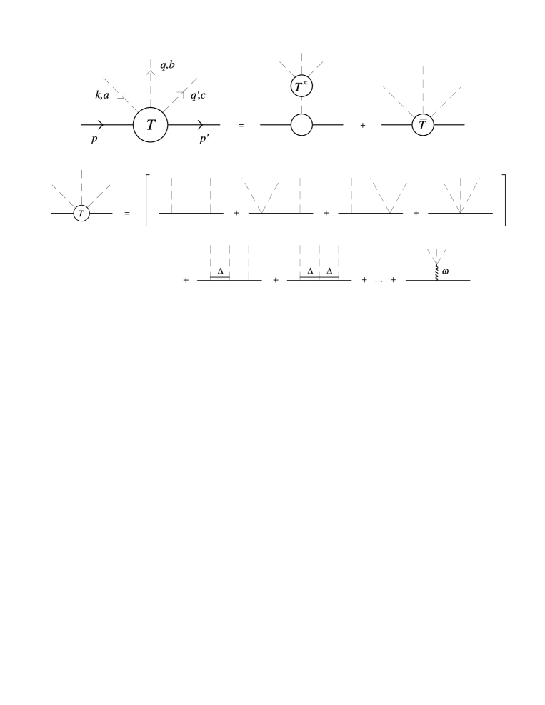
FIG. 1.: Diagram for pion production.

There are many alternative ways of implementing chiral symmetry. In particular, the subset of diagrams in the pure pion-nucleon sector, corresponding to the minimal realization of chiral symmetry in this problem, may be evaluated by means of non-linear Lagrangians with $\pi$N couplings that may be either pseudovector (PV) os pseudoscalar (PS). Denoting the pion field by $\phi$, and defining $f=(f_{\pi}^{2}-\mbox{\boldmath$\phi$}^{2})^{1/2}$, we have

$${\cal L}_{PV} = {\cal L}_{\pi}\!+\!\bar{\psi}\left\{i\gamma_{\mu}\left[\partial^{\mu}\!+\!i\frac{\mbox{\boldmath$\phi$}\times\partial^{\mu}\mbox{\boldmath$\phi$}}{f_{\pi}(f\!+\!f_{\pi})}\cdot\frac{\mbox{\boldmath$\tau$}}{2}\right]\!-\!m\right\}\psi\!+\!\frac{g_{A}}{2f_{\pi}}\bar{\psi}\gamma_{\mu}\gamma_{5}\mbox{\boldmath$\tau$}\psi\!\cdot\!\left(\partial^{\mu}\mbox{\boldmath$\phi$}-\frac{\partial^{\mu}f\mbox{\boldmath$\phi$}}{f+f_{\pi}}\right)\;,$$ (1)

$${\cal L}_{PS} = {\cal L}_{\pi}+\bar{N}i\not\!\partial N-g\bar{N}(f+i\mbox{\boldmath$\tau$}\cdot\mbox{\boldmath$\phi$}\gamma_{5})N\;,$$ (2)

where

$${\cal L}_{\pi}=\left[\frac{1}{2}(\partial_{\mu}f\partial^{\mu}f\!+\!\partial_{\mu}\mbox{\boldmath$\phi$}\!\cdot\!\partial^{\mu}\mbox{\boldmath$\phi$})\!+\!f_{\pi}\mu^{2}f\right]\!\;.$$ (3)

In these expressions, $\psi$ and $N$ are the nucleon fields with non-linear and linear transformation properties, $\mu$ and $m$ are the pion and nucleon masses and $f_{\pi}$, $g$ and $g_{A}$ are respectively the pion decay, the $\pi$N coupling and the axial decay constants. It is important to stress that these Lagrangians, in spite of their different aspects, have the same dynamical content and physical results do not depend on the particular version one adopts, as demonstrated on general grounds [13].

The pion production amplitude has the general form

$$iT_{cba}=\bar{u}\left[\delta_{bc}\tau_{a}\;(A^{\pi}+\bar{A})+\delta_{ac}\tau_{b}\;(B^{\pi}+\bar{B})+\delta_{ab}\tau_{c}\;(C^{\pi}+\bar{C})+i\epsilon_{cba}\;\bar{E}\right]\!\gamma_{5}\;u\;,$$ (4)

where the tags $\pi$ and $bar$ refer to the pion-pole and background contributions. At threshold, this amplitude is usually written as

$$\left.iT_{cba}\right]^{th}=2m\;\mbox{\boldmath$\sigma$}\!\cdot\!\mbox{\boldmath$k$}\left[D_{1}\left(\delta_{ac}\tau_{b}+\delta_{ba}\tau_{c}\right)+D_{2}\;\delta_{cb}\tau_{a}\right]\;,$$ (5)

where $D_{1}$ and $D_{2}$ are dynamical coefficients. Their empirical values may be obtained from the following specific processes

$$(\pi^{-}p\rightarrow\pi^{+}\pi^{-}n)\rightarrow\left.iT\right]^{th} = 2\sqrt{2}\;m\;\mbox{\boldmath$\sigma$}\!\cdot\!\mbox{\boldmath$k$}\;D_{1}\;,$$ (6)

$$(\pi^{+}p\rightarrow\pi^{+}\pi^{+}n)\rightarrow\left.iT\right]^{th} = \sqrt{2}\;m\;\mbox{\boldmath$\sigma$}\!\cdot\!\mbox{\boldmath$k$}\;\left(D_{1}+D_{2}\right)\;.$$ (7)

The pion-pole amplitude for on-shell nucleons is

$$iT_{cba}^{\pi}=-\;\frac{mg_{A}}{f_{\pi}}\;\left[\bar{u}\;\tau_{d}\;\gamma_{5}\;u\right]\frac{T_{dcba}^{\pi\pi}}{(p^{\prime}\!-\!p)^{2}-\mu^{2}}\;,$$ (8)

where $T_{dcba}^{\pi\pi}$ is the pion scattering amplitude. At tree level, it is given by

$$T_{dcba}^{\pi\pi}=\frac{1}{f_{\pi}^{2}}\;\left\{\delta_{ad}\delta_{bc}\left[(q\!+\!q^{\prime})^{2}\!-\!\mu^{2}\right]\!+\!\delta_{bd}\delta_{ac}\left[(k\!-\!q^{\prime})^{2}\!-\!\mu^{2}\right]\!+\!\delta_{cd}\delta_{ab}\left[(k\!-\!q)^{2}\!-\!\mu^{2}\right]\right\}$$ (9)

and yields

$$A^{\pi}=-\;\frac{mg_{A}}{f_{\pi}^{3}}\;\frac{(p^{\prime}\!-\!p\!-\!k)^{2}-\mu^{2}}{(p^{\prime}\!-\!p)^{2}-\mu^{2}}\;.$$ (10)

The contributions to $\bar{A}$, calculated with the PV Lagrangian, are given by

$$\bar{A} = \left(\frac{mg_{A}}{f_{\pi}}\right)^{3}\left\{\frac{\not\!{q}^{\prime}\not\!{k}}{(q^{\prime 2}\!+\!2p^{\prime}\!\cdot\!q^{\prime})(k^{2}\!+\!2p\!\cdot\!k)}+\frac{\not\!{k}\not\!{q}^{\prime}}{(k^{2}\!-\!2p^{\prime}\!\cdot\!k)(q^{\prime 2}\!-\!2p\!\cdot\!q^{\prime})}+\frac{\not\!{q}\not\!{k}}{(q^{2}\!+\!2p^{\prime}\!\cdot\!q)(k^{2}\!+\!2p\!\cdot\!k)}\right.$$ (11)

$$+ \left.\frac{\not\!{k}\not\!{q}}{(k^{2}\!-\!2p^{\prime}\!\cdot\!k)(q^{2}\!-\!2p\!\cdot\!q)}+\frac{\not\!{q}^{\prime}\not\!{q}}{(q^{\prime 2}\!+\!2p^{\prime}\!\cdot\!q^{\prime})(q^{2}\!-\!2p\!\cdot\!q)}+\frac{\not\!{q}\not\!{q}^{\prime}}{(q^{2}\!+\!2p^{\prime}\!\cdot\!q)(q^{\prime 2}\!-\!2p\!\cdot\!q^{\prime})}\right.$$ (12)

$$- \left.\;\frac{1}{m}\left(\frac{\not\!{k}}{k^{2}\!+\!2p\!\cdot\!k}+\frac{\not\!{k}}{k^{2}\!-\!2p^{\prime}\!\cdot\!k}\right)\right.$$ (13)

$$+ \left.\frac{1-1/g_{A}^{2}}{4m^{2}}\left[-2\;\frac{\not\!{k}}{m}+\frac{(\not\!{k}\!+\!\not\!{q}^{\prime})\not\!{q}}{q^{2}\!-\!2p\!\cdot\!q}+\frac{(\not\!{k}\!+\!\not\!{q})\not\!{q}^{\prime}}{q^{\prime 2}\!-\!2p\!\cdot\!q^{\prime}}+\frac{\not\!{q}(\not\!{k}\!+\!\not\!{q}^{\prime})}{q^{2}\!+\!2p^{\prime}\!\cdot\!q}+\frac{\not\!{q}^{\prime}(\not\!{k}\!+\!\not\!{q})}{q^{\prime 2}\!+\!2p^{\prime}\!\cdot\!q^{\prime}}\right]\right\}\;,$$ (14)

the corresponding expressions for $B$ and $C$ are obtained by making $k\rightarrow-q$ and $k\rightarrow-q^{\prime}$ respectively, and $\bar{E}$ is

$$\bar{E} = \left(\frac{mg_{A}}{f_{\pi}}\right)^{3}\left\{\frac{\not\!{q}^{\prime}\not\!{k}}{(q^{\prime 2}\!+\!2\,p^{\prime}\!\cdot\!q^{\prime})(k^{2}\!+\!2p\!\cdot\!k)}-\frac{\not\!{k}\not\!{q}^{\prime}}{(k^{2}\!-\!2p^{\prime}\!\cdot\!k)(q^{\prime 2}\!-\!2p\!\cdot\!q^{\prime})}-\frac{\not\!{q}\not\!{k}}{(q^{2}\!+\!2p^{\prime}\!\cdot\!q)(k^{2}\!+\!2p\!\cdot\!k)}\right.$$ (15)

$$+ \left.\frac{\not\!{k}\not\!{q}}{(k^{2}\!-\!2p^{\prime}\!\cdot\!k)(q^{2}\!-\!2p\!\cdot\!q)}+\frac{\not\!{q}^{\prime}\not\!{q}}{(q^{\prime 2}\!+\!2p^{\prime}\!\cdot\!q^{\prime})(q^{2}\!-\!2p\!\cdot\!q)}-\frac{\not\!{q}\not\!{q}^{\prime}}{(q^{2}\!+\!2p^{\prime}\!\cdot\!q)(q^{\prime 2}\!-\!2p\!\cdot\!q^{\prime})}\right\}\;.$$ (16)

For future purposes, one notes that if the PS Lagrangian were used, one would obtain the same structure with $g_{A}=1$ and the last line of the eq. for $\bar{A}$ would vanish. In the PS case, the signature of chiral symmetry are the contact interactions due to the function $f$ in eq.(2), which give rise to the terms proportional to $1/m$ in eq.(14).

In order to estimate the accuracy of the pion-production amplitude derived from eq.(1), we consider the contributions to the amplitudes $D_{1}$ and $D_{2}$, which are written in terms of the variables

$$D_{1}^{\pi} = \frac{g_{A}}{2f_{\pi}^{3}}\;\sqrt{\frac{2m}{E\!+\!m}}\;\frac{\mu\;(2\omega\!-\!\mu)}{2m(E\!-\!m)\!+\!\mu^{2}}\;,$$ (17)

$$\bar{D}_{1} = -\frac{g_{A}^{3}}{4f_{\pi}^{3}}\sqrt{\frac{2m}{E\!+\!m}}\left[\frac{2m}{2m\!+\!\mu}\!\left(1\!-\frac{\mu}{2E\!-\!\mu}\right)\!-\!\left(1\!-\frac{1}{g_{A}^{2}}\right)\!\left(1\!-\frac{\mu}{m}-\frac{\mu}{2E\!-\!\mu}+\frac{\mu}{2m\!+\!\mu}\right)\right],$$ (18)

and

$$D_{2}^{\pi} = -\;\frac{g_{A}}{2f_{\pi}^{3}}\;\sqrt{\frac{2m}{E\!+\!m}}\;\frac{3\mu^{2}}{2m(E\!-\!m)\!+\!\mu^{2}}\;,$$ (19)

$$\bar{D}_{2} = -\;\frac{g_{A}^{3}}{4f_{\pi}^{3}}\sqrt{\frac{2m}{E+m}}\,\left[\frac{4m^{2}}{2m\omega\!-\!\mu^{2}}\left(\frac{\mu}{m}+\frac{\mu}{2E\!-\!\mu}\right)-\frac{m}{2m\!+\!\mu}\left(1+\frac{4m}{2E\!-\!\mu}\right)\right.$$ (20)

$$- \left.2\left(1-\frac{1}{g_{A}^{2}}\right)\left(\frac{\mu}{m}+\frac{\mu}{2E\!-\!\mu}-\frac{\mu}{2m\!+\!\mu}\right)\right]\;,$$ (21)

where $\omega=[\mu(4m\!+\!5\mu)]/[2(m\!+\!2\mu)]$ and $E=m\!+\!2\mu\!-\!\omega$. Expanding these amplitudes in powers of $\mu/m$, one has

$$D_{1} = [D_{1}^{\pi}]+[\bar{D}_{1}]\simeq\left[\frac{g_{A}}{8f_{\pi}^{3}}\;\left(3+\frac{3}{2}\;\frac{\mu}{m}+\cdots\right)\right]-\left[\frac{g_{A}}{8f_{\pi}^{3}}\left(2-2\;\frac{\mu}{m}+\cdots\right)\right]\;,$$ (22)

$$D_{2} = [D_{2}^{\pi}]+[\bar{D}_{2}]\simeq-\left[\frac{g_{A}}{8f_{\pi}^{3}}\left(3+\frac{9}{2}\;\frac{\mu}{m}+\cdots\right)\right]-\left[\frac{g_{A}}{8f_{\pi}^{3}}\left(4\;\frac{\mu}{m}+\cdots\right)\right]\;.$$ (24)

The results for the full amplitudes at threshold, namely $D_{1}=g_{A}(1+7\mu/2m)/8f_{\pi}^{3}$ and $D_{2}=-g_{A}(3+17\mu/2m)/8f_{\pi}^{3}$, coincide with those obtained in the framework of chiral perturbation theory [14]. In order to asses the role of chiral symmetry in this problem we note that a Lagrangian without any symmetry, containing just a PS $\pi$N interaction, would give rise to the same pion-pole contribution and an amplitude $\bar{A}$ corresponding to just the six first terms in eq.(14), which involve two nucleon propagators. Therefore the full elimination of chiral symmetry would yield $\bar{D}_{1}\rightarrow g_{A}(2)/8f_{\pi}^{3}$ and $\bar{D}_{2}\rightarrow-g_{A}(-4+3\mu/m)/8f_{\pi}^{3}$, indicating that chiral symmetry does play a role in this problem. On the other hand, that this role is not as large as in the case of $\pi$N$\rightarrow\pi$N, where the same procedure would change one of the scattering lenghts by a factor of 200. Numerical results for the amplitudes are given in table I and show that predictions from the minimal chiral model are close to empirical values, although there is some room for improvement in $D_{2}$.

TABLE I.: Subamplitudes $D_{1}$ and $D_{2}$ in $\mu^{-3}$ units. Experimental results correspond to a best fit quoted in ref.[12].

	$D_{1}^{\pi}$	$\bar{D}_{1}$	$D_{1}$	$D_{2}^{\pi}$	$\bar{D}_{2}$	$D_{2}$
eqs.($\ref{2.12}-\ref{2.15}$)	1.78	-0.91	0.87	-2.02	-0.30	-2.32
CHPT, eqs.(22,24)	1.81	-0.96	0.85	-2.06	-0.33	-2.39
experiment	-	-	0.80	-	-	-3.20

In this work we are interested in the construction of the NN interaction due to the exchange of three pions, which is based on the amplitude $\bar{T}_{cba}$. As indicated in fig.3, the complete evaluation of this amplitude would require the calculation of a large number of diagrams. However, long ago Olsson and Turner [15] have shown that the leading contribution to this amplitude comes from the effective Lagrangian

$$\bar{\cal{L}}=\frac{g_{A}}{8f_{\pi}^{3}}\;\bar{\psi}\gamma_{\mu}\;\gamma_{5}\mbox{\boldmath$\tau$}\;\psi\!\cdot\!\mbox{\boldmath$\phi$}\;\partial^{\mu}\mbox{\boldmath$\phi$}^{2}\;.$$ (25)

It gives rise to the following contribution to $\bar{A}$

$$\bar{A}=\frac{2g_{A}}{8f_{\pi}^{3}}\left(2m-\not\!{k}\right)\;$$ (26)

and, as before, $\bar{B}$ and $\bar{C}$ are obtained by making $k\rightarrow-q$ and $k\rightarrow-q^{\prime}$ respectively. This corresponds to the threshold amplitudes

$$\bar{D}_{1} = -\;\frac{g_{A}}{8f_{\pi}^{3}}\;\sqrt{\frac{2m}{E\!+\!m}}\;\left(2+\frac{\mu}{m}\right)\simeq-\;\frac{g_{A}}{8f_{\pi}^{3}}\left(2+\frac{\mu}{m}\right)\;,$$ (27)

$$\bar{D}_{2} = \;\frac{g_{A}}{8f_{\pi}^{3}}\;\sqrt{\frac{2m}{E\!+\!m}}\;\left(\frac{2\mu}{m}\right)\simeq\frac{g_{A}}{8f_{\pi}^{3}}\left(\frac{2\mu}{m}\right)\;,$$ (28)

showing that the effective Lagrangian given by eq.(25) reproduces correctly the leading contribution at threshold.

III Nucleon-Nucleon Interaction

The basic element in the construction of the NN potential due to the exchange of three uncorrelated pions (3PEP) is the corresponding Born amplitude for the process N$(p_{1})$N$(p_{2})\rightarrow$N$(p_{1}^{\prime})$N$(p_{2}^{\prime})$, associated with the diagrams of figure 2. Denoting this amplitude by $F$, one has

$$F=\frac{1}{3!}\int\frac{d^{4}Q}{(2\pi)^{4}}\int\frac{d^{4}Q^{\prime}}{(2\pi)^{4}}\;\Delta(k)\;\Delta(q)\;\Delta(q^{\prime})\;\;\bar{T}_{cba}^{(1)}\;\;\bar{T}_{cba}^{(2)}\;,$$ (29)

where the factor $1/3!$ is due to the symmetry of the intermediate three-pion state, $\Delta$ is a pion propagator and $\bar{T}_{cba}^{(i)}$ is the pion production amplitude for nucleon $i$.

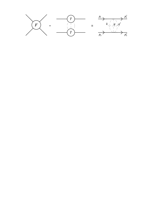
FIG. 2.: Leading contribution to the three-pion exchange potential.

We adopt the following external kinematic variables

$$W = p_{1}+p_{2}=p^{\prime}_{1}+p^{\prime}_{2}\;,$$ (30)

$$\Delta = p^{\prime}_{1}-p_{1}=p_{2}-p^{\prime}_{2}\;,$$ (31)

$$z = [(p_{1}+p^{\prime}_{1})-(p_{2}+p^{\prime}_{2})]/2\;.$$ (32)

As the nucleons are assumed to be on-shell, they are constrained by

$$W\!\cdot\!z=W\!\cdot\!\Delta=z\!\cdot\!\Delta=0\;.$$ (33)

For the internal variables we define

$$Q = (q+q^{\prime}+k)/2\;,$$ (34)

$$Q^{\prime} = (q^{\prime}-q)/2\;,$$ (35)

so that

$$k = Q-\Delta/2\;,$$ (36)

$$q = Q/2+\Delta/4-Q^{\prime}\;,$$ (37)

$$q^{\prime} = Q/2+\Delta/4+Q^{\prime}$$ (38)

and the condition of momentum conservation reads $q+q^{\prime}-k=\Delta$.

As discussed in the previous section, the leading contribution to the amplitude $\bar{T}$ comes from the effective Lagrangian given by eq.(25), which yields the following intermediate effective vertex for nucleon (2)

$$\bar{T}_{cba}^{(2)}=i\left(\frac{g_{A}}{4f_{\pi}^{3}}\right)\left(\bar{u}\gamma^{\mu}\gamma_{5}u\right)^{(2)}\left[\delta_{bc}\tau_{a}^{(2)}\;(q+q^{\prime})_{\mu}+\delta_{ac}\tau_{b}^{(2)}\;(q^{\prime}-k)_{\mu}+\delta_{ab}\tau_{c}^{(2)}\;(q-k)_{\mu}\right]\;.$$ (39)

The corresponding expression for nucleon (1) has the same form, but is globally multiplied by (-1), due to the senses of flow of internal momenta. Using these results into eq.(29), we have

$$F(\Delta)=\left(\frac{g_{A}}{4f_{\pi}^{3}}\right)^{2}\;\mbox{\boldmath$\tau$}^{(1)}\!\cdot\!\mbox{\boldmath$\tau$}^{(2)}\;\left(\bar{u}\gamma^{\mu}\gamma_{5}u\right)^{(1)}\left(\bar{u}\gamma^{\nu}\gamma_{5}u\right)^{(2)}\;I_{\mu\nu}(\Delta)\;,$$ (40)

where $I_{\mu\nu}$ is given by

$$I_{\mu\nu}(\Delta) = \frac{1}{3!}\;\int\frac{d^{4}Q}{(2\pi)^{4}}\;\frac{1}{[(Q\!-\!\Delta/2)^{2}\!-\!\mu^{2}]}$$ (41)

$$\times \int\frac{d^{4}Q^{\prime}}{(2\pi)^{4}}\;\frac{[3Q_{\mu}Q_{\nu}\!-\!Q_{\mu}\Delta_{\nu}/2\!-\!\Delta_{\mu}Q_{\nu}/2\!+\!27\Delta_{\mu}\Delta_{\nu}/4+4Q^{\prime}_{\mu}Q^{\prime}_{\nu}]}{[(Q^{\prime}\!-\!Q/2\!-\!\Delta/4)^{2}\!-\!\mu^{2}][(Q^{\prime}\!+\!Q/2\!+\!\Delta/4)^{2}\!-\!\mu^{2}]}\;.$$ (42)

This function is evaluated in the appendix and reads

$$I_{\mu\nu}=\Delta_{\mu}\Delta_{\nu}\;\mu^{4}\;I^{p}(\Delta)+g_{\mu\nu}\;\mu^{6}\;I^{a}(\Delta)\;,$$ (43)

with $I^{p}$ and $I^{a}$ given by eqs.(A27) and (A29) respectively. Using the nucleon equation of motion, one has

$$F(\Delta)=-\left(\frac{\;g_{A}}{4f_{\pi}^{3}}\right)^{2}\mbox{\boldmath$\tau$}^{(1)}\!\cdot\mbox{\boldmath$\tau$}^{(2)} \left[\;4m^{2}\mu^{4}\;\left(\bar{u}\gamma_{5}u\right)^{(1)}\left(\bar{u}\gamma_{5}u\right)^{(2)}\;I^{p}(\Delta)\right.$$ (45)

$$-\left.\mu^{6}\;\left(\bar{u}\gamma^{\mu}\gamma_{5}u\right)^{(1)}\left(\bar{u}\gamma_{\mu}\gamma_{5}u\right)^{(2)}\;I^{a}(\Delta)\right]\;.$$

This expression corresponds to the exchanges of pseudoscalar and axial systems. In order to make the strength of the interaction more transparent, we eliminate $g_{A}$ in favour of $g$, by means of the G-T relation, $g_{A}=gf_{\pi}/m$, and write

$$F(\Delta)=-\;g^{2}\;\mbox{\boldmath$\tau$}^{(1)}\!\cdot\mbox{\boldmath$\tau$}^{(2)}\left(\frac{\mu^{2}}{2f_{\pi}^{2}}\right)^{2} \left[\left(\bar{u}\gamma_{5}u\right)^{(1)}\left(\bar{u}\gamma_{5}u\right)^{(2)}\;I^{p}(\Delta)\right.$$ (47)

$$-\left.\frac{\mu^{2}}{4m^{2}}\left(\bar{u}\gamma^{\mu}\gamma_{5}u\right)^{(1)}\left(\bar{u}\gamma_{\mu}\gamma_{5}u\right)^{(2)}\;I^{a}(\Delta)\right]\;.$$

For future purposes, it is worth noting that the corresponding amplitude for one-pion exchange is

$$F^{\pi}(\Delta)=-\;g^{2}\;\mbox{\boldmath$\tau$}^{(1)}\!\cdot\mbox{\boldmath$\tau$}^{(2)}\left[\left(\bar{u}\gamma_{5}u\right)^{(1)}\left(\bar{u}\gamma_{5}u\right)^{(2)}\;\frac{1}{\Delta^{2}-\mu^{2}}\right]\;.$$ (48)

Going to the non-relativistic limit in the center of mass frame, one has

$$\frac{F(\mbox{\boldmath$\Delta$})}{4m^{2}}\rightarrow f(\mbox{\boldmath$\Delta$})=-\left(\frac{g}{2m}\right)^{2}\mbox{\boldmath$\tau$}^{(1)}\!\cdot\mbox{\boldmath$\tau$}^{(2)}\left(\frac{\mu^{2}}{2f_{\pi}^{2}}\right)^{2} \left[-\mbox{\boldmath$\sigma$}^{(1)}\!\cdot\!\mbox{\boldmath$\Delta$}\;\mbox{\boldmath$\sigma$}^{(2)}\!\cdot\!\mbox{\boldmath$\Delta$}\;I^{p}(\Delta)\right.$$ (50)

$$+\left.\mu^{2}\;\mbox{\boldmath$\sigma$}^{(1)}\!\cdot\!\mbox{\boldmath$\sigma$}^{(2)}\;I^{a}(\Delta)\right]\;.$$

This result allows the configuration space potential to be written as

$$V^{3\pi}(x) = -\;\frac{\mu}{4\pi}\;\int\frac{d^{3}\mbox{\boldmath$\Delta$}}{(2\pi)^{3}}\;e^{-i\mbox{\boldmath$\Delta$}\cdot\mbox{\boldmath$r$}}\left[\frac{4\pi}{\mu}\;f(\mbox{\boldmath$\Delta$})\right]$$ (51)

$$= \left(\frac{g\mu}{2m}\;\frac{\mu^{2}}{2f_{\pi}^{2}}\right)^{2}\frac{\mu}{4\pi}\mbox{\boldmath$\tau$}^{(1)}\!\cdot\mbox{\boldmath$\tau$}^{(2)}\left[\mbox{\boldmath$\sigma$}^{(1)}\!\cdot\!\mbox{\boldmath$\nabla$}_{x}\;\mbox{\boldmath$\sigma$}^{(2)}\!\cdot\!\mbox{\boldmath$\nabla$}_{x}\;U^{p}(x)+\mbox{\boldmath$\sigma$}^{(1)}\!\cdot\!\mbox{\boldmath$\sigma$}^{(2)}\;U^{a}(x)\right]\;,$$ (52)

where the $U(x)$ are integrals of Yukawa functions, written in terms of the variable $x\equiv\mu r$ and given by eqs.(A38) and (A40).

Using the result

$$\mbox{\boldmath$\sigma$}^{(1)}\!\cdot\!\mbox{\boldmath$\nabla$}_{x}\mbox{\boldmath$\sigma$}^{(2)}\!\cdot\!\mbox{\boldmath$\nabla$}_{x} \left[\left(1+\frac{3}{ax}+\frac{3}{a^{2}x^{2}}\right)\frac{e^{-ax}}{x^{3}}\right]=\frac{a^{2}}{3}\left[\mbox{\boldmath$\sigma$}^{(1)}\!\cdot\mbox{\boldmath$\sigma$}^{(2)}\left(1+\frac{7}{ax}+\frac{27}{a^{2}x^{2}}+\frac{60}{a^{3}x^{3}}+\frac{60}{a^{4}x^{4}}\right)\right.$$ (54)

$$+\left.S_{12}\left(1+\frac{10}{ax}+\frac{45}{a^{2}x^{2}}+\frac{105}{a^{3}x^{3}}+\frac{105}{a^{4}x^{4}}\right)\right]\frac{e^{-ax}}{x^{3}}\;,$$

with $S_{12}=3\mbox{\boldmath$\sigma$}^{(1)}\!\cdot\!\hat{\mbox{\boldmath$x$}}\;\mbox{\boldmath$\sigma$}^{(2)}\!\cdot\!\hat{\mbox{\boldmath$x$}}-\mbox{\boldmath$\sigma$}^{(1)}\!\cdot\!\mbox{\boldmath$\sigma$}^{(2)}$, into eqs.(A38) and (A40), we obtain

$$V^{3\pi}(r) = \frac{1}{3}\left(\frac{g\mu^{3}}{4mf_{\pi}^{2}}\right)^{2}\frac{\mu}{4\pi}\;\mbox{\boldmath$\tau$}^{(1)}\!\cdot\mbox{\boldmath$\tau$}^{(2)}\left\{\mbox{\boldmath$\sigma$}^{(1)}\!\cdot\!\mbox{\boldmath$\sigma$}^{(2)}\left[U_{0}^{p}(x)+3\;U^{a}(x)\right]+S_{12}\;U_{2}^{p}(x)\right\}\;,$$ (55)

where

$$U_{0}^{p}(x) = \frac{1}{(4\pi)^{4}}\;\frac{1}{6}\int_{0}^{1}\!d\alpha\int_{0}^{1}\!d\gamma\;\gamma\;a^{4}\;\left\{[3\!+\!(1\!-\!2\alpha)^{2}](1\!-\!2\gamma)^{2}+2[1\!-\!(1\!-\!2\alpha)^{2}](1\!-\!2\gamma)\right.$$ (56)

$$+ \left.[27\!+\!(1\!-\!2\alpha)^{2}]\right\}\left(1+\frac{7}{ax}+\frac{27}{a^{2}x^{2}}+\frac{60}{a^{3}x^{3}}+\frac{60}{a^{4}x^{4}}\right)\;\frac{e^{-ax}}{x^{3}}\;,$$ (57)

$$U_{2}^{p}(x) = \frac{1}{(4\pi)^{4}}\;\frac{1}{6}\int_{0}^{1}\!d\alpha\int_{0}^{1}\!d\gamma\;\gamma\;a^{4}\;\left\{[3\!+\!(1\!-\!2\alpha)^{2}](1\!-\!2\gamma)^{2}+2[1\!-\!(1\!-\!2\alpha)^{2}](1\!-\!2\gamma)\right.$$ (58)

$$+ \left.[27\!+\!(1\!-\!2\alpha)^{2}]\right\}\left(1+\frac{10}{ax}+\frac{45}{a^{2}x^{2}}+\frac{105}{a^{3}x^{3}}+\frac{105}{a^{4}x^{4}}\right)\;\frac{e^{-ax}}{x^{3}}\;,$$ (59)

$$U^{a}(x) = -\;\frac{1}{(4\pi)^{4}}\;\frac{8}{3}\int_{0}^{1}\!d\alpha\int_{0}^{1}\!d\gamma\;\alpha(1-\alpha)\gamma^{3}(1-\gamma)\;a^{5}\;$$ (60)

$$\times \left(1+\frac{6}{ax}+\frac{15}{a^{2}x^{2}}+\frac{15}{a^{3}x^{3}}\right)\;\frac{e^{-ax}}{x^{4}}$$ (61)

and

$$a=\sqrt{\frac{1}{1-\gamma}+\frac{4}{\gamma[1-(1-2\alpha)^{2}]}}\;.$$ (62)

The structure of this result is similar to that of the OPEP, which is given by

$$V^{\pi}(r) = \frac{1}{3}\left(\frac{g\mu}{2m}\right)^{2}\frac{\mu}{4\pi}\mbox{\boldmath$\tau$}^{(1)}\!\cdot\mbox{\boldmath$\tau$}^{(2)}\left\{\mbox{\boldmath$\sigma$}^{(1)}\!\cdot\!\mbox{\boldmath$\sigma$}^{(2)}\left(\frac{e^{-x}}{x}\right)+S_{12}\left[\left(1+\frac{3}{x}+\frac{3}{x^{2}}\right)\frac{e^{-x}}{x}\right]\right\}\;.$$ (63)

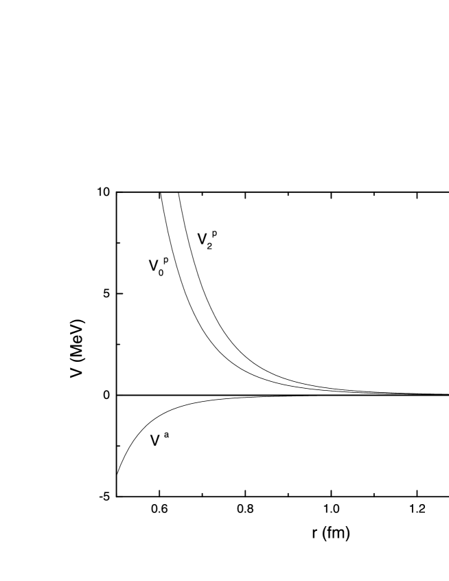
FIG. 3.: Profile function for the $V_{0}^{p}$, $V_{2}^{p}$ and $V^{a}$ component of the three-pion exchange potential.

The profile functions of the spin-spin and tensor components of the three-pion exchange potential are displayed in fig.3, where it is possible to note that all the curves show the typical divergent behaviour of unregularized potentials at the origin. Therefore we assume that our results are realistic for internucleon distances larger than 0.7 fm, the usual bag radius. Inspecting the figure for the spin-spin chanel, one learns that the contribution of the axial component is quite small and hence the three-pion exchange potential is dominated by the pseudoscalar channel. In both $V_{SS}$ and $V_{T}$ its contribution tends to add to the OPEP and is visible up to 1.5 fm, as shown in fig.4. The influence of this component of the force over observables will be discussed elsewhere.

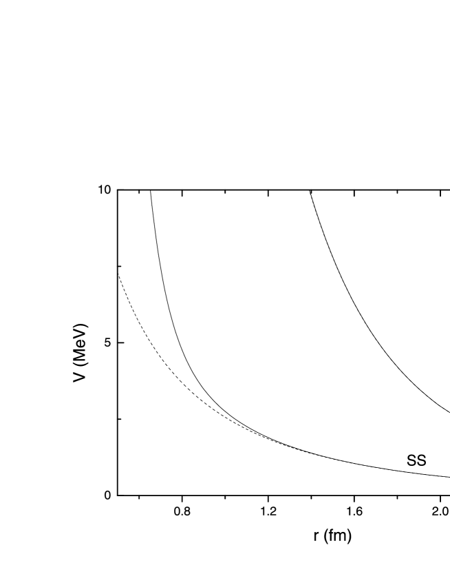
FIG. 4.: Profile function for the spin-spin (SS) and tensor (T) components of the $V^{\pi}$ (dashed line) and $V^{\pi}+V^{3\pi}$ (solid line).

In order to produce a feeling for the structure of the functions $U(x)$, in the appendix we have evaluated approximately the integrals in eqs.(57-61) and obtained the following asymptotic results ($x\rightarrow\infty$)

$$U_{0}^{p}(x) \rightarrow \frac{\pi}{(4\pi)^{4}}\;\frac{80}{\sqrt{3}}\left(1+\frac{3}{x}+\frac{13}{3x^{2}}+\frac{10}{3x^{3}}+\frac{10}{9x^{4}}\right)\;\frac{e^{-3x}}{x^{4}}\;,$$ (64)

$$U_{2}^{p}(x) \rightarrow \frac{\pi}{(4\pi)^{4}}\;\frac{80}{\sqrt{3}}\left(1+\frac{4}{x}+\frac{20}{3x^{2}}+\frac{16}{3x^{3}}+\frac{16}{9x^{4}}\right)\;\frac{e^{-3x}}{x^{4}}\;,$$ (65)

$$U^{a}(x) \rightarrow -\;\frac{\pi}{(4\pi)^{4}}\;\frac{16}{3\sqrt{3}}\left(1+\frac{2}{x}+\frac{5}{3x^{2}}+\frac{5}{9x^{3}}\right)\;\frac{e^{-3x}}{x^{5}}\;,$$ (66)

which are compared with the exact ones in fig.5.

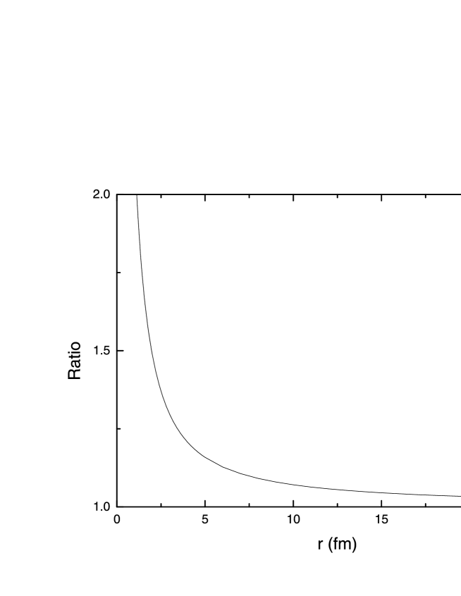
FIG. 5.: Ratios between the approximate expressions (64-66) by the corresponding functions (57-61) - all ratios are identical.

A last point we would like to address here concerns the nature of the force in the chiral limit. The potential given in eqs.(55-62) incorporates two kinds of approximations. The first of them is associated with the assumption that ${\bar{\mathcal{L}}}$, eq.(25), represents the leading contribution to the NN$\pi\pi\pi$ vertex. The other one is related to the non-relativistic limit taken in eq.(50). On the other hand, no approximations besides the neglect of contact interactions were performed in the calculation of the three-pion propagator represented by the functions $I(\Delta)$. Therefore the corresponding configuration space expressions, given by eqs.(57-61) also do not contain approximations and can be used to evaluate the form of the interaction in the chiral limit. The strength of $V^{3\pi}(r)$, as given by eq.(55), is proportional to $\mu^{7}$. Recalling that $x=\mu r$, we obtain the following results when $\mu\rightarrow 0$: $\mu^{7}U_{0}^{p}(x)\rightarrow 140/[(4\pi)^{4}\;r^{7}]$, $\mu^{7}U_{2}^{p}(x)\rightarrow 245/[(4\pi)^{4}\;r^{7}]$ and $\mu^{7}U^{a}(x)\rightarrow-5/[(4\pi)^{4}\;r^{7}]$. Thus, the three-pion exchange NN potential survives in the chiral limit, where it has the form

$$V^{3\pi}(r) \rightarrow \frac{1}{3}\left(\frac{g}{4mf_{\pi}^{2}}\right)^{2}\frac{1}{(4\pi)^{5}}\;\mbox{\boldmath$\tau$}^{(1)}\!\cdot\mbox{\boldmath$\tau$}^{(2)}\left[125\;\mbox{\boldmath$\sigma$}^{(1)}\!\cdot\!\mbox{\boldmath$\sigma$}^{(2)}+245\;S_{12}\right]\;\frac{1}{r^{7}}\;.$$ (67)

acknowledgment

J.C.P. would like to thank FAPESP for financial support.

A Integrals

In this appendix we evaluate the integral $I_{\mu\nu}$ given by eq.(42), using the following results

$$X(K;\mu,\xi)=\int\frac{d^{4}Q}{(2\pi)^{4}}\;\frac{1}{[(Q\!-\!K/2)^{2}\!-\!\mu^{2}]\;[(Q\!+\!K/2)^{2}\!-\!\mu^{2}\xi^{2}]}$$ (A1)

$$=\frac{i}{(4\pi)^{2}}\int_{0}^{1}\!d\alpha\left[\rho_{0}\!-\!\ln\left(1\!-\frac{K^{2}}{\mu^{2}\Sigma^{2}}\right)\right]\;,$$ (A2)

$$X_{\mu}(K;\mu,\xi)=\int\frac{d^{4}Q}{(2\pi)^{4}}\;\frac{Q_{\mu}}{[(Q\!-\!K/2)^{2}\!-\!\mu^{2}]\;[(Q\!+\!K/2)^{2}\!-\!\mu^{2}\xi^{2}]}$$ (A3)

$$=-\;\frac{i}{(4\pi)^{2}}K_{\mu}\int_{0}^{1}\!d\alpha\left(\frac{1-2\alpha}{2}\right)\left[\rho_{0}\!-\!\ln\left(1\!-\frac{K^{2}}{\mu^{2}\Sigma^{2}}\right)\right]\;,$$ (A4)

$$X_{\mu\nu}(K;\mu,\xi)=\int\frac{d^{4}Q}{(2\pi)^{4}}\;\frac{Q_{\mu}Q_{\nu}}{[(Q\!-\!K/2)^{2}\!-\!\mu^{2}]\;[(Q\!+\!K/2)^{2}\!-\!\mu^{2}\xi^{2}]}$$ (A5)

$$=\frac{i}{(4\pi)^{2}}\left\{K_{\mu}K_{\nu}\int_{0}^{1}\!d\alpha\left(\frac{1-2\alpha}{2}\right)^{2}\left[\rho_{0}\!-\!\ln\left(1\!-\frac{K^{2}}{\mu^{2}\Sigma^{2}}\right)\right]\right.$$ (A6)

$$+\left.\frac{\mu^{2}}{2}\;g_{\mu\nu}\int_{0}^{1}\!d\alpha\;\frac{\Sigma^{2}[1\!-\!(1\!-\!2\alpha)^{2}]}{4}\left(1\!-\frac{K^{2}}{\mu^{2}\Sigma^{2}}\right)\left[\rho_{1}\!-\!\ln\left(1\!-\frac{K^{2}}{\mu^{2}\Sigma^{2}}\right)\right]\right\}\;,$$ (A7)

where

$$\Sigma^{2}=\frac{4[\alpha+(1-\alpha)\xi^{2}]}{[1-(1-2\alpha)^{2}]}\;,$$ (A8)

$\rho_{0}$ and $\rho_{1}$ are constants associated with the dimensional regularization procedure. In order to perform the integrations, it is convenient to use the following representation for the logarithm

$$\ln\left(1-\frac{K^{2}}{\mu^{2}\Sigma^{2}}\right)=\int_{0}^{1}\!d\beta\;\left(\frac{1}{\beta}+\frac{\mu^{2}\Sigma^{2}/\beta^{2}}{K^{2}-\mu^{2}\Sigma^{2}/\beta}\right)\;.$$ (A9)

Quite generally, constants appearing in these results correspond to contact interactions, since they do not depend on $\Delta$. As we are interested in the long range part of the potential, these constants will be neglected in the sequence and we write

$$X(K;\mu,\xi) = -\;\frac{i}{(4\pi)^{2}}\int_{0}^{1}\!d\alpha\int_{0}^{1}\!d\beta\;\frac{\mu^{2}\Sigma^{2}/\beta^{2}}{K^{2}\!-\!\mu^{2}\Sigma^{2}/\beta}\;,$$ (A10)

$$X_{\mu}(K;\mu,\xi) = \frac{i}{(4\pi)^{2}}\int_{0}^{1}\!d\alpha\int_{0}^{1}\!d\beta\;\frac{\mu^{2}\Sigma^{2}/\beta^{2}}{K^{2}\!-\!\mu^{2}\Sigma^{2}/\beta}\left[\left(\frac{1\!-\!2\alpha}{2}\right)K_{\mu}\right]\;,$$ (A11)

$$X_{\mu\nu}(K;\mu,\xi) = -\;\frac{i}{(4\pi)^{2}}\int_{0}^{1}\!d\alpha\int_{0}^{1}\!d\beta\;\frac{\mu^{2}\Sigma^{2}/\beta^{2}}{K^{2}\!-\!\mu^{2}\Sigma^{2}/\beta}\left\{\left(\frac{1\!-\!2\alpha}{2}\right)^{2}K_{\mu}K_{\nu}\right.$$ (A12)

$$- \left.\left[\frac{\Sigma^{2}[1\!-\!(1\!-\!2\alpha)^{2}](1\!-\!\beta)}{8\beta}\right]\;\mu^{2}\;g_{\mu\nu}\right\}\;.$$ (A13)

The integral in $Q^{\prime}$ can be performed using these results and one has

$$I^{\prime}_{\mu\nu} = \int\frac{d^{4}Q^{\prime}}{(2\pi)^{4}}\;\frac{[3Q_{\mu}Q_{\nu}\!-\!Q_{\mu}\Delta_{\nu}/2\!-\!\Delta_{\mu}Q_{\nu}/2\!+\!27\Delta_{\mu}\Delta_{\nu}/4+4Q^{\prime}_{\mu}Q^{\prime}_{\nu}]}{[(Q^{\prime}\!-\!Q/2\!-\!\Delta/4)^{2}\!-\!\mu^{2}][(Q^{\prime}\!+\!Q/2\!+\!\Delta/4)^{2}\!-\!\mu^{2}]}$$ (A14)

$$= (3Q_{\mu}Q_{\nu}\!-\!Q_{\mu}\Delta_{\nu}/2\!-\!\Delta_{\mu}Q_{\nu}/2\!+\!27\Delta_{\mu}\Delta_{\nu}/4)/\mu^{2}\;X(Q\!+\!\Delta/2;\mu,1)$$ (A15)

$$+ 4\;X_{\mu\nu}(Q\!+\!\Delta/2;\mu,1)$$ (A16)

$$= -\;\frac{i}{(4\pi)^{2}}\;\mu^{2}\;\int_{0}^{1}\!d\alpha\int_{0}^{1}\!d\beta\;\frac{\lambda^{2}}{\beta}\;\frac{1}{[(Q\!+\!\Delta/2)^{2}\!-\!\mu^{2}\lambda^{2}]}\left\{[3\!+\!(1\!-\!2\alpha)^{2}]\;Q_{\mu}Q_{\nu}\right.$$ (A17)

$$- \left.[1\!-\!(1\!-\!2\alpha)^{2}](Q_{\mu}\Delta_{\nu}\!+\!\Delta_{\mu}Q_{\nu})/2+[27\!+\!(1\!-\!2\alpha)^{2}]\;\Delta_{\mu}\Delta_{\nu}/4\right.$$ (A18)

$$- \left.\lambda^{2}[1\!-\!(1\!-\!2\alpha)^{2}](1\!-\!\beta)\;\mu^{2}\;g_{\mu\nu}/2\right\}\;,$$ (A19)

where

$$\lambda^{2}=\frac{4}{\beta[1-(1-2\alpha)^{2}]}\;.$$ (A20)

The function $I_{\mu\nu}$ is then given by

$$I_{\mu\nu}(\Delta)=\frac{1}{3!}\;\int\frac{d^{4}Q}{(2\pi)^{4}}\;\frac{1}{[(Q-\Delta/2)^{2}\!-\!\mu^{2}]}\;I^{\prime}_{\mu\nu}$$ (A21)

$$=-\;\frac{i}{(4\pi)^{2}}\frac{1}{3!}\;\mu^{2}\int_{0}^{1}\!d\alpha\int_{0}^{1}\!d\beta\;\frac{\lambda^{2}}{\beta}\left\{[3\!+\!(1\!-\!2\alpha)^{2}]\;X_{\mu\nu}(\Delta,\mu,\lambda)\right.$$ (A22)

$$-\left.[1\!-\!(1\!-\!2\alpha)^{2}]\;[\Delta_{\mu}X_{\nu}(\Delta,\mu,\lambda)\!+\!\Delta_{\nu}X_{\mu}(\Delta,\mu,\lambda)]/2+[27\!+\!(1\!-\!2\alpha)^{2}]X(\Delta,\mu,\lambda)\;\Delta_{\mu}\Delta_{\nu}/4\right.$$ (A23)

$$-\left.\lambda^{2}[1\!-\!(1\!-\!2\alpha)^{2}](1\!-\!\beta)\;X(\Delta,\mu,\lambda)\;\mu^{2}\;g_{\mu\nu}/2\right\}$$ (A24)

$$=\Delta_{\mu}\Delta_{\nu}\;\mu^{4}\;I^{p}(\Delta)+g_{\mu\nu}\;\mu^{6}\;I^{a}(\Delta)\;,$$ (A25)

where

$$I^{p}(\Delta) = -\;\frac{1}{(4\pi)^{4}}\;\frac{1}{24}\int_{0}^{1}\!d\alpha\int_{0}^{1}\!d\beta\int_{0}^{1}\!d\gamma\int_{0}^{1}\!d\epsilon\;\frac{\lambda^{2}\theta^{2}}{\beta\epsilon}\left\{[3\!+\!(1\!-\!2\alpha)^{2}](1\!-\!2\gamma)^{2}\right.$$ (A26)

$$+ \left.2[1\!-\!(1\!-\!2\alpha)^{2}](1\!-\!2\gamma)+[27\!+\!(1\!-\!2\alpha)^{2}]\right\}\;\frac{1}{[\Delta^{2}\!-\!\mu^{2}\theta^{2}]}\;,$$ (A27)

$$I^{a}(\Delta) = \frac{1}{(4\pi)^{4}}\;\frac{1}{48}\int_{0}^{1}\!d\alpha\int_{0}^{1}\!d\beta\int_{0}^{1}\!d\gamma\int_{0}^{1}\!d\epsilon\;\frac{\lambda^{2}\theta^{2}}{\beta\epsilon}\left\{4\;\lambda^{2}\;[1\!-\!(1\!-\!2\alpha)^{2}](1\!-\!\beta)\right.$$ (A28)

$$+ \left.\theta^{2}\;[3\!+\!(1\!-\!2\alpha)^{2}][1\!-\!(1\!-\!2\gamma)^{2}](1\!-\!\epsilon)\right\}\;\frac{1}{[\Delta^{2}\!-\!\mu^{2}\theta^{2}]}\;,$$ (A29)

with

$$\theta^{2}=\frac{4[\gamma+(1-\gamma)\lambda^{2}]}{\epsilon[1-(1-2\gamma)^{2}]}\;.$$ (A30)

Results presented in this appendix are covariant. On the other hand, the calculation of the potential is performed in the centre of mass of the NN system and we use $\Delta=(0;\mbox{\boldmath$\Delta$})\rightarrow\Delta^{2}=-\mbox{\boldmath$\Delta$}^{2}$.

The potential in configuration space is determined by the functions $U(x)$, given by

$$U(x)=\frac{4\pi}{\mu}\int\frac{d^{3}\mbox{\boldmath$\Delta$}}{(2\pi)^{3}}\;e^{-i\mbox{\boldmath$\Delta$}\cdot\mbox{\boldmath$r$}}\;I(\Delta)\;.$$ (A31)

where $x\equiv\mu r$. Using the result

$$\int\frac{d^{3}\mbox{\boldmath$\Delta$}}{(2\pi)^{3}}\;\frac{e^{-i\mbox{\boldmath$\Delta$}\cdot\mbox{\boldmath$r$}}}{\mbox{\boldmath$\Delta$}^{2}+\mu^{2}\theta^{2}}=\frac{\mu}{4\pi}\;\frac{e^{-\theta x}}{x}\;,$$ (A32)

we have

$$U^{p}(x) = \frac{1}{(4\pi)^{4}}\;\frac{1}{24}\int_{0}^{1}\!d\alpha\int_{0}^{1}\!d\beta\int_{0}^{1}\!d\gamma\int_{0}^{1}\!d\epsilon\;\frac{\lambda^{2}\theta^{2}}{\beta\epsilon}\left\{[3\!+\!(1\!-\!2\alpha)^{2}](1\!-\!2\gamma)^{2}\right.$$ (A33)

$$+ \left.2[1\!-\!(1\!-\!2\alpha)^{2}](1\!-\!2\gamma)+[27\!+\!(1\!-\!2\alpha)^{2}]\right\}\;\frac{e^{-\theta x}}{x}\;,$$ (A34)

$$U^{a}(x) = -\;\frac{1}{(4\pi)^{4}}\;\frac{1}{48}\int_{0}^{1}\!d\alpha\int_{0}^{1}\!d\beta\int_{0}^{1}\!d\gamma\int_{0}^{1}\!d\epsilon\;\frac{\lambda^{2}\theta^{2}}{\beta\epsilon}\left\{4\;\lambda^{2}\;[1\!-\!(1\!-\!2\alpha)^{2}](1\!-\!\beta)\right.$$ (A35)

$$+ \left.\theta^{2}\;[3\!+\!(1\!-\!2\alpha)^{2}][1\!-\!(1\!-\!2\gamma)^{2}](1\!-\!\epsilon)\right\}\;\frac{e^{-\theta x}}{x}\;.$$ (A36)

The integrations in $\epsilon$ and $\beta$ can be performed analytically and we have

$$U^{p}(x) = \frac{1}{(4\pi)^{4}}\;\frac{1}{6}\int_{0}^{1}\!d\alpha\int_{0}^{1}\!d\gamma\;\gamma\;a^{2}\;\left\{[3\!+\!(1\!-\!2\alpha)^{2}](1\!-\!2\gamma)^{2}+2[1\!-\!(1\!-\!2\alpha)^{2}](1\!-\!2\gamma)\right.$$ (A37)

$$+ \left.[27\!+\!(1\!-\!2\alpha)^{2}]\right\}\left(1+\frac{3}{ax}+\frac{3}{a^{2}x^{2}}\right)\;\frac{e^{-ax}}{x^{3}}\;,$$ (A38)

$$U^{a}(x) = -\;\frac{1}{(4\pi)^{4}}\;\frac{8}{3}\int_{0}^{1}\!d\alpha\int_{0}^{1}\!d\gamma\;\alpha(1-\alpha)\gamma^{3}(1-\gamma)\;a^{5}\;$$ (A39)

$$\times \left(1+\frac{6}{ax}+\frac{15}{a^{2}x^{2}}+\frac{15}{a^{3}x^{3}}\right)\;\frac{e^{-ax}}{x^{4}}\;,$$ (A40)

where

$$a=\sqrt{\frac{1}{1-\gamma}+\frac{4}{\gamma[1-(1-2\alpha)^{2}]}}\;.$$ (A41)

The integrals over $\alpha$ and $\gamma$ can be evaluated approximately for large values of $x$. In this case, the exponential has a sharp minimum for $\alpha=1/2,\gamma=2/3$ and varies very rapidly around it. Thus all the elements in the integrand but the exponential may be taken as constants and we have

$$U^{p}(x) = \frac{1}{(4\pi)^{4}}\;\frac{80}{3}\left(1+\frac{1}{x}+\frac{1}{3x^{2}}\right)\;\frac{1}{x^{3}}\int_{0}^{1}\!d\alpha\int_{0}^{1}\!d\gamma\;e^{-ax}\;,$$ (A42)

$$U^{a}(x) = -\;\frac{1}{(4\pi)^{4}}\;16\left(1+\frac{2}{x}+\frac{5}{3x^{2}}+\frac{5}{9x^{3}}\right)\;\frac{1}{x^{4}}\int_{0}^{1}\!d\alpha\int_{0}^{1}\!d\gamma\;e^{-ax}\;.$$ (A43)

In order to perform the last integral we first use a new variable $u$, related to $\alpha$ by

$$\alpha=\frac{1}{2}-\left[\frac{1}{4}-\frac{1}{4+2\gamma u^{2}\sqrt{\frac{4-3\gamma}{\gamma(1-\gamma)}}+\gamma u^{4}}\right]^{1/2}$$ (A44)

and then another variable $v$, related to $\gamma$ by

$$\gamma=\frac{3+\left(3+v^{2}\right)^{2}\mp\sqrt{48v^{2}+44v^{2}+12v^{6}+v^{8}}}{2\left(3+v^{2}\right)^{2}}\;,$$ (A45)

where the ($-$) and ($+$) signs refer to the intervals $0\leq\gamma\leq 2/3$ and $2/3\leq\gamma\leq 1$ respectively. We then obtain

$$\int_{0}^{1}\!d\alpha\int_{0}^{1}\!d\gamma\;e^{-ax}=\frac{\pi}{3\sqrt{3}}\;\frac{e^{-3x}}{x}\;.$$ (A46)

REFERENCES

[1]
[2] H. Yukawa, Proc. Phys. Math. Soc. Japan 17, 48
(1935); M. Taketani, S. Nakamura and M. Sasaki, Progr. Theor. Phys.
VI, 581 (1951).
[3] T. Hamada and J.D. Johnston, Nucl. Phys. 34, 382 (1962);
Y. Nakamura and R. Tamagaki, Progr. Theor. Phys. 33, 769 (1965);
K.E. Lassila, M.H. Hull, H.M. Ruppel, F.A. MacDonald and G.E. Breit,
Phys. Rev. 126, 881 (1962); R.V. Reid, Ann. Phys. (N.Y.)
50, 411 (1968).
[4] W.N. Cottingham and R. Vinh Mau, Phys. Rev. 130, 735 (1963);
W.N. Cottingham, M. Lacombe, B. Loiseau, J.M. Richard and R. Vinh Mau,
Phys. Rev. D8, 800 (1973);
M. Lacombe, B. Loiseau, J.M. Richard, R. Vinh Mau, J. Coté, P. Pires
and R. de Tourreil, Phys. Rev. C21, 861 (1980).
[5] R. Machleidt, K. Holinde and Ch. Elster, Phys. Lett. C149, 1
(1987).
[6] G. Höhler, group I, vol.9, subvol.b, part 2 of Landölt-Bornstein Numerical data and Functional Relationships
in Science and Technology, ed. H.Schopper, 1983.
[7] C. Ordóñez and U. van Kolck, Phys. Lett. B291,
459 (1992).
[8] L.S. Celenza, A. Pantziris and C.M. Shakin, Phys. Rev. C46,
2213 (1992); J.L. Friar and S.A. Coon, Phys. Rev. C49, 1272 (1994);
C.A.da Rocha and M.R. Robilotta, Phys. Rev. C49, 1818 (1994); M.C.
Birse, Phys. Rev. C49, 2212 (1994);
[9] C. Ordóñez, L. Ray and U. van Kolck, Phys. Rev. Lett.
72, 1982 (1994); Phys. Rev. C 53, 2086 (1996);
M.R. Robilotta, Nucl. Phys. A595, 171 (1995);
M.R. Robilotta and C.A. da Rocha, Nucl. Phys A615, 391 (1997).
[10] N. Kaiser, R. Brockman and W. Weise, Nucl. Phys. A 625, 758
(1997);
N. Kaiser, S. Gertendörfer and W. Weise, preprint nucl-th/9802071;
J-L. Ballot, M.R. Robilotta and C.A. da Rocha, Phys. Rev. C57, 1574
(1998).
[11] M.R. Robilotta, proceedings of the XX Reunião de Trabalho em
Física Nuclear no Brasil (1997), ed. C.L. Lima; proceedings of the VI
Workshop on Hadron Physics (1998), ed. F.F.S. Cruz and S. Avancini.
[12] J. Heitzmann, Thèse de 3ème cycle, L’Université
Pierre et Marie Curie (1979), unpublished.
[13] S. Coleman, J. Wess and B. Zumino, Phys. Rev. 177, 2239
(1969); G. Callan, S. Coleman, J. Wess and B. Zumino, Phys. Rev. 177,
2247 (1969).
[14] V. Bernard, N. Kaiser and U. Meissner, Int. J. Mod. Phys.
E 4, 193 (1995).
[15] M.G. Olsson and L. Turner, Phys. Rev. Let. 20, 1127 (1968).