Electron scattering on two–neutron halo nuclei: The case of ⁶He

Abstract

The formalism to describe electron scattering reactions on two–neutron halo nuclei is developed. The halo nucleus is described as a three–body system (core+n+n), and the wave function is obtained by solving the Faddeev equations in coordinate space. We discuss elastic and quasielastic scattering using the impulse approximation to describe the reaction mechanism. We apply the method to investigate the case of electron scattering on ⁶He. Spectral functions, response functions, and differential cross sections are calculated for both neutron knockout and $\alpha$ knockout by the electron.

PACS numbers: 25.30.Fj, 25.60.-t, 25.70.Bc, 21.45.+v

I Introduction

In the middle of the 80’s it was experimentally found that some light nuclei close to the neutron drip line have an spatial extension much larger than expected according to its mass number [1, 2, 3, 4]. This is the case for instance of ¹¹Li, that has a root mean square radius similar to a nucleus with a mass number three times larger. Very soon it was suggested that these nuclei could be understood as a core surrounded by one or more neutrons, which extend to several times the nuclear radius [5]. This picture was supported by subsequent studies that proved the validity of the few–body models as an appropriate method to describe the most general properties of halo nuclei [6, 7, 8, 9, 10].

The term halo nuclei has then been coined to describe very weakly bound and spatially extended systems, where several (usually one or two) neutrons have a high probability of being at distances larger than the typical nuclear radius. For a general overview of their basic properties see for instance [11]. Among halo nuclei a lot of attention has been paid to two–neutron halo systems from which ⁶He ($\alpha+n+n$) and ¹¹Li (⁹Li $+n+n$) are their maximum exponents [12]. They are samples of the so called Borromean nuclei, that have the property of being bound while all the two–body subsystems made by two of the three constituents are unbound.

The ability to produce secondary beams of halo nuclei opened the possibility of investigating their structure by the measurement of the momentum distributions of the fragments coming out after a collision with stable nuclei [13, 14, 15, 16, 17, 18, 19]. The simplest approach to the understanding of Borromean nuclei fragmentation reactions was made by means of the sudden approximation [20, 21, 22], that assumes that one of the three particles in the projectile is instantaneously removed by the target, while the other two particles remain undisturbed. Clearly this can only be justified for reaction times much shorter than the characteristic time for the motion of the three particles in the system. Since the system is weakly bound this requirement is well fulfilled for a high energy beam. This model was proved to be valid to describe the core momentum distributions [22], but it failed in the attempt of reproducing experimental momentum distributions for neutrons. Several authors suggested that the final interaction between the two non–disturbed particles played an essential role, especially when low–lying resonances are present [16, 21, 23]. Incorporation into the model of the final state interaction [24, 25] is in fact necessary in order to obtain a good agreement between theory and experiment also for neutron momentum distributions. Indeed further refinements [26, 27] in the description of the reaction process have been proved to be crucial for a better interpretation of the experimental data.

Although a lot of information has been extracted from the halo nucleus–nucleus fragmentation reactions, it may pay to look for cleaner ways of investigating the structure of halo nuclei. As in any nucleus–nucleus collision the effects of the strong interaction involved in the reaction mechanism are mixed with those determining the nuclear structure. It is very well known that the way to avoid this problem is to substitute the hadron probe by electrons. In fact electron scattering is usually considered as the most powerful tool to investigate nuclear structure [28, 29]. The electromagnetic coupling constant is small enough such that the Born approximation can be used, the electron–nucleus interaction is well described through QED, and it is possible to vary independently the momentum transfer and the energy transfer to the nucleus. The problem when dealing with halo nuclei is that they are far from the stability region, and the nuclear target can not be at rest as in conventional nuclear structure studies with electron beams. However it is in principle possible to perform electron scattering experiments by means of the collision between a secondary beam of unstable nuclei and an electron beam. This kind of experiments are part of the MUSES (MultiUSse Experimental Storage rings) project in RIKEN, and they are projected for the beginning of the coming century [30].

In parallel with the experimental projects it is then clear that theoretical studies of the process should be developed. From the experimental point of view the simplest reaction would be the elastic scattering. This would permit to investigate the charge density of the halo nucleus. This is specially interesting when the proton dripline is approached because it directly gives the extension of the possible proton halo (⁸B is a good candidate for this). For neutron halos the charge radius is expected to be the one of the core. Elastic electron scattering on ¹¹Li or ⁶He will be important to confirm that this picture of neutron halo nuclei is correct. As one slightly increases the energy transfer to the nucleus the halo will break up, and coincidence $(e,e^{\prime}x)$ measurements can be made, with $x$ either a halo neutron or the stable core.

The main goal of this paper is to contribute to the first steps in the investigation of electron scattering reactions on two–neutron halo nuclei. To illustrate the model we will consider the case of electron–⁶He scattering. Although estimates of the elastic scattering reaction will be given, most of the work will be devoted to $(e,e^{\prime}n)$ and $(e,e^{\prime}\alpha)$ reactions at quasielastic kinematics.

The paper is organized as follows: A brief description of kinematics and of elastic scattering reactions is given in sections II and III, respectively. The differential cross section for exclusive $(e,e^{\prime}x)$ processes is given in section IV. Sections V and VI are devoted to the theoretical description of the different ingredients involved in the electron–⁶He scattering process and to the presentation of the results, respectively. Concluding remarks are given in section VII.

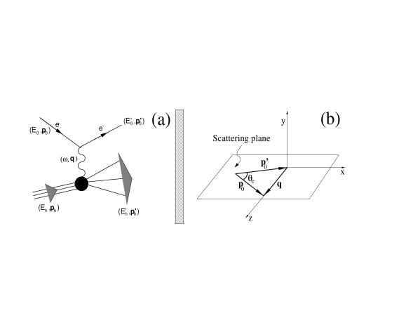
FIG. 1.: (a) Scheme of a general electron–nucleus reaction in the Born approximation. (b) Axes system chosen to describe the process.

II Kinematics and general considerations

In fig.1a we show the scheme of a general electron scattering reaction. An electron with energy and momentum $(E_{0},\mbox{\boldmath$p$}_{0})$ hits a target with energy and momentum $(E_{h},\mbox{\boldmath$p$}_{h})$. The energy and momentum transfer to the nucleus is denoted by $(\omega,\mbox{\boldmath$q$})$, and the energy and momentum of the scattered electron and the final nuclear system are given by $(E^{\prime}_{0},\mbox{\boldmath$p$}^{\prime}_{0})$ and $(E^{\prime}_{h},\mbox{\boldmath$p$}^{\prime}_{h})$, respectively.

In fig.1b we show our axis system. The $z$–axis is chosen along the momentum transfer $q$. The $y$–axis is defined along $\mbox{\boldmath$p$}_{0}\times\mbox{\boldmath$p$}^{\prime}_{0}$, and it is therefore perpendicular to the scattering plane defined by $\mbox{\boldmath$p$}_{0}$ and $\mbox{\boldmath$p$}^{\prime}_{0}$. The $x$–axis is defined by $\hat{\mbox{\boldmath$y$}}\times\hat{\mbox{\boldmath$z$}}$, where $\hat{\mbox{\boldmath$z$}}$ and $\hat{\mbox{\boldmath$y$}}$ are unit vectors along the $z$–axis and $y$–axis, respectively. The angle between $\mbox{\boldmath$p$}_{0}$ and $\mbox{\boldmath$p$}^{\prime}_{0}$ is the scattering angle $\theta_{e}$.

Energy and momentum conservation in the process determine that

$$E_{0}+E_{h} = E^{\prime}_{0}+E^{\prime}_{h}$$ (1)

$$\mbox{\boldmath$p$}_{0}+\mbox{\boldmath$p$}_{h} = \mbox{\boldmath$p$}^{\prime}_{0}+\mbox{\boldmath$p$}^{\prime}_{h}$$ (2)

and the energy and momentum transfer are related to the electron and nuclear energy and momentum by

$$\omega = E_{0}-E^{\prime}_{0}=E^{\prime}_{h}-E_{h}$$ (3)

$$q = \mbox{\boldmath$p$}_{0}-\mbox{\boldmath$p$}^{\prime}_{0}=\mbox{\boldmath$p$}^{\prime}_{h}-\mbox{\boldmath$p$}_{h}$$ (4)

Working in the frame of the nucleus ($E_{h}=M_{h}$ and $\mbox{\boldmath$p$}_{h}=0$) these expressions can be rewritten as

$$\omega+M_{h}=E^{\prime}_{h};\hskip 28.45274pt\mbox{\boldmath$q$}=\mbox{\boldmath$p$}^{\prime}_{h}$$ (5)

and the invariant hadronic mass ($W$) takes the form

$$W^{2}=E^{\prime 2}_{h}-\mbox{\boldmath$p$}^{\prime 2}_{h}=(\omega+M_{h})^{2}-\mbox{\boldmath$q$}^{2}$$ (6)

From eq.(4) we obtain that

$$Q^{2}=-q_{\mu}^{2}=\mbox{\boldmath$q$}^{2}-\omega^{2}=4E_{0}E^{\prime}_{0}\sin^{2}\frac{\theta_{e}}{2}$$ (7)

where ultrarelativistic electrons have been assumed (the electron mass is neglected).

In the case of elastic scattering the invariant hadronic mass coincides with the mass of the target ($W=M_{h}$), and eq.(6) leads to

$$\omega=(M_{h}^{2}+q^{2})^{1/2}-M_{h}=E^{\prime}_{h}-M_{h}=T_{h}$$ (8)

that is the kinetic energy of the final nucleus:

$$\omega=T_{h}=\frac{Q^{2}}{2M_{h}}$$ (9)

Assuming that the two–neutron halo nucleus has no excited bound states (as it happens in ⁶He) an increase of the energy transfer to the nucleus will break the halo system into its three constituents. The energy and momentum of the final hadronic system can then be written as

$$E^{\prime}_{h} = E^{\prime}_{1}+E^{\prime}_{2}+E^{\prime}_{3}$$ (10)

$$\mbox{\boldmath$p$}^{\prime}_{h} = \mbox{\boldmath$p$}^{\prime}_{1}+\mbox{\boldmath$p$}^{\prime}_{2}+\mbox{\boldmath$p$}^{\prime}_{3}$$ (11)

where $(E_{i},\mbox{\boldmath$p$}^{\prime}_{i})$ ($i=1,2,3$) are the energy and momentum of the three fragments. eqs. (2) to (6) are then valid in this region after substitution on them of eq. (11). Processes involving excitations and one nucleon knockout from the core may take place at higher energies, and will not be discussed here.

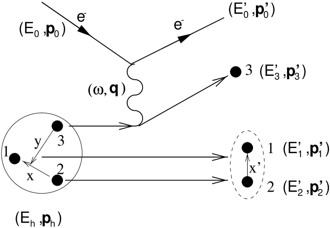
FIG. 2.: Scheme of the reaction and definition of the coordinates used to describe the exclusive $(e,e^{\prime}x)$ process on a two–neutron halo nucleus. Only one of the constituents of the halo nucleus is considered to interact with the electron.

These breakup processes will be studied assuming that the whole energy and momentum transfer are absorbed by one of the constituents (participant), which is knocked out from the halo system. The other two constituents are mere spectators. The large extension of the nucleus supports this picture, since the probability for simultaneous interaction with the electron of two of the nuclear constituents is small. The scheme of the reaction can be seen in fig.2. If we consider constituent 3 as the participant one, we then have

$$E^{\prime}_{3} = E_{3}+\omega$$ (12)

$$\mbox{\boldmath$p$}^{\prime}_{3} = \mbox{\boldmath$p$}_{3}+\mbox{\boldmath$q$}$$ (13)

$$E_{h}-E_{3} = E^{\prime}_{1}+E^{\prime}_{2}$$ (14)

$$\mbox{\boldmath$p$}_{h}-\mbox{\boldmath$p$}_{3} = \mbox{\boldmath$p$}^{\prime}_{1}+\mbox{\boldmath$p$}^{\prime}_{2}$$ (15)

where $(E_{3},\mbox{\boldmath$p$}_{3})$ are the energy and momentum of the participant constituent inside the halo nucleus.

In the target frame ($E_{h}=M_{h}$ and $\mbox{\boldmath$p$}_{h}=0$) we have that $\mbox{\boldmath$p$}_{3}=-(\mbox{\boldmath$p$}^{\prime}_{1}+\mbox{\boldmath$p$}^{\prime}_{2})$, and

$$\omega+M_{h}=E^{\prime}_{h}=m_{1}+m_{2}+m_{3}+T_{1}+T_{2}+T_{3}.$$ (16)

Assuming non relativistic kinetic energies for the three fragments we have

$$\omega-B_{h}=\frac{p^{\prime 2}_{1}}{2m_{1}}+\frac{p^{\prime 2}_{2}}{2m_{2}}+\frac{p^{\prime 2}_{3}}{2m_{3}}=$$ (18)

$$E^{\prime}_{x}+\frac{p_{3}^{2}}{2(m_{1}+m_{2})}+\frac{(\mbox{\boldmath$p$}_{3}+\mbox{\boldmath$q$})^{2}}{2m_{3}}$$

where $B_{h}$ is the halo binding energy, $m_{i}$ and $T_{i}$ are the masses and final kinetic energies of the three constituents of the halo nucleus, and $E^{\prime}_{x}$ is the kinetic energy of the system made by particles 1 and 2 referred to its own center of mass.

From eq.(18) one can see that for a fixed value of the momentum transfer $q$ the variation in the energy transfer $\omega$ is connected to the different values of the internal momentum $\mbox{\boldmath$p$}_{3}$ of the participant particle. Actually, for a fixed value of the momentum transfer, electron–nucleus scattering cross sections show a broad peak known as the quasielastic peak whose center is placed at $\mbox{\boldmath$p$}_{3}=0$. Neglecting the binding energy $B_{h}$ and the internal energy $E^{\prime}_{x}$ we obtain from eq.(18) the following value for the energy transfer in the center of the quasielastic peak

$$\omega_{\mbox{q.p.}}\approx\frac{q^{2}}{2m_{3}}$$ (19)

that corresponds to the kinetic energy transferred to a particle of mass $m_{3}$ at rest. Reactions taking place in a quasielastic peak region are interpreted as processes where a single constituent in the nucleus absorbs the whole energy and momentum transfer, being ejected from the nucleus.

When the participant particle is the core, the center of the quasielastic peak is at smaller energy than when the participant particle is one of the halo neutrons. In the ⁶He case $\omega_{\mbox{q.p.}}$ is approximately four times smaller for a participant ⁴He than for a participant neutron.

In this paper the exclusive $(e,e^{\prime}x)$ reactions will be investigated in the so called perpendicular kinematics, where the energy and momentum transfer are maintained fixed. In this kinematics, for a given electron beam with energy and momentum $(E_{0},\mbox{\boldmath$p$}_{0})$, the scattering angle $\theta_{e}$ and the energy of the outgoing electron $E^{\prime}_{0}$ are fixed during the experiment. From (4) and (7) it is clear that $\theta_{e}$ and $E^{\prime}_{0}$ can be chosen in such a way that $\omega$ and $q$ take the desired values. In particular, for a fixed value of $q$ the energy transfer will be taken as shown in (19). We are then working in the center of a quasielastic peak.

The energy transfer in the center of the quasielastic peak obviously increases with the momentum transfer $q$. If this momentum is such that $\omega$ is larger than the separation energy of the nucleons in core, then a neutron detected in coincidence with the electron could come from the core instead of coming from the halo. Therefore if $\omega$ is maintained below the separation energy of the nucleons in the core we guarantee that the halo nucleus is broken in only its three constituents. In particular, for ⁶He, since the neutron or proton separation energy in ⁴He is around 20 MeV a momentum transfer smaller than 200 MeV/c would satisfy this condition. At the same time a value of $\omega$ below 20 MeV is also unable to excite the $\alpha$ particle to its first excited state.

From eq.(15) and assuming that $E_{3}^{2}=\mbox{\boldmath$p$}_{3}^{2}+m_{3}^{2}$ we can write

$$\left(p_{3}^{2}+q^{2}+2p_{3}q\cos(\theta_{3})+m_{3}^{2}\right)^{1/2}=\left(p_{3}^{2}+m_{3}^{2}\right)^{1/2}+\omega$$ (20)

If we now take $q=200$ MeV/c and let the energy transfer take the value $q^{2}/2m_{\alpha}$ ($\omega\approx 5$ MeV), it is then simple to see from eq.(20) that this energy can be absorbed by a participant $\alpha$ particle ($m_{3}=m_{\alpha}$) with rather low internal momentum (smaller than a few MeV/c). If for the same value of $\omega$ we consider that the participant particle is one of the halo neutrons ($m_{3}=m_{n}$) the required internal momentum of the neutron has to be very large (typically of several hundreds of MeV/c). However the probability of finding a halo neutron in ⁶He with such a large momentum is basically zero [21, 26]. In the same way, from eq.(20) one sees that if $\omega=q^{2}/2m_{n}$ ($\omega\approx 20$ MeV for $q=200$ MeV/c) a participant neutron with small momentum can absorb such an energy, but it can not be absorbed by a participant $\alpha$ particle.

Therefore, assuming that the reaction picture shown in fig.2 is valid (a single constituent acts as participant while the other two are just spectators), we can then conclude that an energy transfer in the center of the $\alpha$ quasielastic peak ($\omega=q^{2}/2m_{\alpha})$ selects the $\alpha$ as participant particle, and a halo neutron if $\omega$ is in the center of the neutron quasielastic peak ($\omega=q^{2}/2m_{n})$.

III Elastic scattering

The general expression for the elastic electron scattering cross section can be found for instance in [31]. In particular for a nucleus with spin zero, as ⁶He, the elastic cross section in the nucleus frame takes the form

$$\frac{d\sigma}{d\Omega_{e}}=\frac{Z^{2}\sigma_{M}}{f_{rec}}\frac{Q^{4}}{q^{4}}|F_{ch}(q)|^{2}$$ (21)

where the ultrarelativistic limit for the electrons has been assumed, $\Omega_{e}$ defines the direction of the outgoing electron, and

$$\sigma_{M}=\frac{\alpha^{2}\cos^{2}{(\theta_{e}/2)}}{4E_{0}^{2}\sin^{4}{(\theta_{e}/2)}};\hskip 8.5359ptf_{rec}=1+\frac{2E_{0}\sin{(\theta_{e}/2)}}{M_{h}}$$ (22)

are the Mott cross section and the recoil factor.

The charge form factor $F_{ch}(q)$ is given by

$$F_{ch}(q)=\frac{4\pi}{Z}\int\frac{\sin(qr)}{qr}\rho(r)r^{2}dr$$ (23)

where $\rho(r)$ is the charge density.

Assuming that the picture of a core plus several halo neutrons is valid to describe neutron halo nuclei, the charge density should be practically identical to the one of the core. Therefore, since the neutron contribution to the charge form factor will be negligible at moderate $q$–values, the charge form factor should be the one obtained in an elastic electron–core scattering process.

FIG. 3.: Charge form factor after elastic electron scattering from ⁶He assuming that the charge density corresponds to the $\alpha$ charge density (solid line), and assuming that charge is spread out over the whole ⁶He nucleus (dashed line). The inset shows the charge density used in both cases.

To simplify the analysis we take the experimental charge density of ⁴He that can be found in table V of [32]. The root mean square radius of the charge distribution is 1.68 fm, and the charge form factor is shown in fig.3 by the solid line. This should then be the charge form factor obtained after elastic electron scattering on ⁶He provided that the three–body picture is correct.

The other limit would be to consider that the charge is not contained only in the core but distributed like matter over the whole nucleus. In that case the charge form factor would be the one shown in fig.3 by the dashed line. The form factor is now narrower due to the larger value of the charge radius. This curve has been obtained by modifying the range of the gaussians describing the ⁴He charge density in [32] in order to get a root mean square radius of the charge distribution of 2.5 fm, similar to the size of ⁶He.

From fig.3 we can conclude that elastic electron scattering from ⁶He, or in general from neutron halo nuclei, is an excellent tool to determine to what extent the few–body description is valid. The inset in fig.3 shows the charge density for two cases mentioned above.

Center of mass corrections, also contained in the recoil factor of eq.(21), may slightly modify the form factor and the charge r.m.s. radius of ⁶He relative to that of ⁴He. These effects could be accounted for using the three–body wave functions employed in the next sections. However, to give a first estimate of the size of the differential cross sections the two extreme pictures presented in fig.3 serve the purpose. For instance, for $E_{0}\approx 200$ MeV and $\theta_{e}\approx 30$ degrees, the differential cross section is of around 100 $\mu b$.

IV Quasielastic scattering

In this section we enter in the study of the coincidence $(e,e^{\prime}x)$ processes, with $x$ either a halo neutron or the core. The scheme of the reaction was shown in fig.2. A three–body system with energy and momentum $(E_{h},\mbox{\boldmath$p$}_{h})$ interacts with an electron with energy and momentum $(E_{0},\mbox{\boldmath$p$}_{0})$. The whole energy and momentum transfer $(\omega,\mbox{\boldmath$q$})$ is absorbed by one of the three constituents of the nucleus (constituent 3) that is ejected out from the three-body halo system. The energies and momenta in the final state are denoted by $(E^{\prime}_{i},\mbox{\boldmath$p$}^{\prime}_{i})$ where $i=0$ for the electron and $i=1,2,3$ for the three halo constituents.

Together with the impulse approximation (the virtual photon is absorbed by a single constituent) we also neglect the Coulomb distortion of the ingoing and outgoing electrons. They are then described as plane waves. At the same time the distortion due to the final strong interaction between particle 3 (participant) and the two–body subsystem made by particles 1 and 2 (spectators) is also neglected, and the knocked out constituent is also described as a plane wave. On the contrary, the interaction between particles 1 and 2 is included in the calculation. This interaction is what in refs. [24, 25] is referred to as final state interaction, and plays an essential role in the description of the halo nucleus fragmentation reactions. Our picture is then similar to that described for instance in [33, 34] for $(e,e^{\prime}N)$ reactions in PWIA. The only difference (but important) is that our residual nucleus is an unbound two–body system, while they consider that the residual nucleus is in a well defined bound state.

In appendix A it is shown that working in the frame of the three–body halo nucleus ($\mbox{\boldmath$p$}_{h}=\mbox{\boldmath$p$}_{1}+\mbox{\boldmath$p$}_{2}+\mbox{\boldmath$p$}_{3}=0$) the transition matrix element of the reaction has the form (A30)

$$S_{fi} = \frac{i}{V^{3}}\frac{e^{2}}{q_{\rho}^{2}}(2\pi)^{17/2}\delta(E_{i}-E_{f})\delta^{3}(\mbox{\boldmath$P$}_{i}-\mbox{\boldmath$P$}_{f})$$ (25)

$$\bar{u}(\mbox{\boldmath$p$}^{\prime}_{0},\sigma^{\prime}_{0})\gamma_{\mu}u(\mbox{\boldmath$p$}_{0},\sigma_{0})\sum_{\sigma_{3}}J^{\mu}_{\sigma_{3}^{\prime},\sigma_{3}}(\mbox{\boldmath$q$},\mbox{\boldmath$p$}_{3})M^{JM}_{s_{12}\sigma_{12},s_{3}\sigma_{3}}(\mbox{\boldmath$p$}^{\prime}_{x},\mbox{\boldmath$p$}^{\prime}_{y})$$

where $E_{i}=E_{0}+E_{h}$ and $E_{f}=E^{\prime}_{0}+E^{\prime}_{1}+E^{\prime}_{2}+E^{\prime}_{3}$ are the initial and final total energies, and analogously for the initial and final total momenta $\mbox{\boldmath$P$}_{i}$ and $\mbox{\boldmath$P$}_{f}$. The Jacobi coordinates $\bf{x}$ and $\bf{y}$ (see fig.2) are defined in (A2) and their conjugated momenta $\mbox{\boldmath$p$}_{x}$ and $\mbox{\boldmath$p$}_{y}$ are given in (A5). The momenta in the final state are denoted with primes. The spinor $u(\mbox{\boldmath$p$},\sigma)$ describes a free electron with momentum $p$ and third spin component $\sigma$. $J^{\mu}_{\sigma_{3}^{\prime},\sigma_{3}}(\mbox{\boldmath$q$},\mbox{\boldmath$p$}_{3})$ is the matrix element in momentum space of the current operator connecting states of the particle 3 with spin projections $\sigma_{3}$ and $\sigma^{\prime}_{3}$ (eq.(A25)). In (eq.(A27)) we have also defined $M^{JM}_{s_{12}\sigma_{12},s_{3}\sigma^{\prime}_{3}}(\mbox{\boldmath$p$}^{\prime}_{x},\mbox{\boldmath$p$}^{\prime}_{y})$, which is the overlap between the initial three–body halo wave function ($\Psi^{JM}(\mbox{\boldmath$x$},\mbox{\boldmath$y$})$) and the continuum wave function of the final two–body subsystem ($w^{s_{12},\sigma_{12}}(\mbox{\boldmath$x$},\mbox{\boldmath$p^{\prime}_{x}$})$). When the interaction between particles 1 and 2 is neglected $M^{JM}_{s_{12}\sigma_{12},s_{3}\sigma^{\prime}_{3}}(\mbox{\boldmath$p$}^{\prime}_{x},\mbox{\boldmath$p$}^{\prime}_{y})$ becomes the Fourier transform (normalized to 1) of the three-body halo wave function. $s_{12}$ and $\sigma_{12}$ are the total spin and its third component of the two–body system made by particles 1 and 2.

We can now compute the differential cross section as the transition probability per unit volume and unit time ($|S_{fi}|^{2}/VT$) divided by the flux of incident particles ($p_{0}/VE_{0}$ in the halo nucleus frame), divided by the number of target particles per unit volume ($1/V$) and multiplied by the number of final states that is given by

$$V\frac{d\mbox{\boldmath$p$}^{\prime}_{0}}{(2\pi)^{3}}V\frac{d\mbox{\boldmath$p$}^{\prime}_{1}}{(2\pi)^{3}}V\frac{d\mbox{\boldmath$p$}^{\prime}_{2}}{(2\pi)^{3}}V\frac{d\mbox{\boldmath$p$}^{\prime}_{3}}{(2\pi)^{3}}=$$ (27)

$$V\frac{d\mbox{\boldmath$p$}^{\prime}_{0}}{(2\pi)^{3}}V\frac{d\mbox{\boldmath$p$}^{\prime}_{3}}{(2\pi)^{3}}V\frac{d\mbox{\boldmath$p$}^{\prime}_{x}}{(2\pi)^{3}}V\frac{d\mbox{\boldmath$p$}^{\prime}_{y}}{(2\pi)^{3}}$$

After averaging over initial states and summing over final states we obtain

$$\frac{d^{12}\sigma}{d\mbox{\boldmath$p$}^{\prime}_{0}d\mbox{\boldmath$p$}^{\prime}_{3}d\mbox{\boldmath$p$}^{\prime}_{x}d\mbox{\boldmath$p$}^{\prime}_{y}} = (2\pi)\frac{e^{4}}{q_{\rho}^{4}}\frac{E_{0}}{p_{0}}\delta(E_{i}-E_{f})\delta(\mbox{\boldmath$P$}_{i}-\mbox{\boldmath$P$}_{f})$$ (30)

$$\frac{1}{2}\sum_{\sigma_{0},\sigma^{\prime}_{0}}|\bar{u}(\mbox{\boldmath$p$}^{\prime}_{0},\sigma^{\prime}_{0})\gamma_{\mu}u(\mbox{\boldmath$p$}_{0},\sigma_{0})|^{2}$$

$$\frac{1}{2J+1}\sum_{M\sigma_{3}}\sum_{s_{12}\sigma_{12}}\left|\sum_{\sigma^{\prime}_{3}}J_{\sigma_{3},\sigma^{\prime}_{3}}^{\mu}(\mbox{\boldmath$q$},\mbox{\boldmath$p$}_{3})M^{JM}_{s_{12}\sigma_{12},s_{3}\sigma_{3}^{\prime}}(\mbox{\boldmath$p$}^{\prime}_{x},\mbox{\boldmath$p$}^{\prime}_{y})\right|^{2}$$

In this expression the integral over $\mbox{\boldmath$p$}^{\prime}_{y}$ can be immediately done by use of the delta of momenta, getting that $\mbox{\boldmath$p$}^{\prime}_{y}=\mbox{\boldmath$q$}-\mbox{\boldmath$p$}^{\prime}_{3}=-\mbox{\boldmath$p$}_{3}$ (see eq.(A24)).

In the ultrarelativistic limit it is known that [35]

$$\frac{1}{2}\sum_{\sigma_{0},\sigma^{\prime}_{0}}|\bar{u}(\mbox{\boldmath$p$}^{\prime}_{0},\sigma^{\prime}_{0})\gamma_{\mu}u(\mbox{\boldmath$p$}_{0},\sigma_{0})|^{2}=\frac{1}{2E_{0}E^{\prime}_{0}}\eta_{\mu\nu}$$ (31)

where the leptonic tensor $\eta_{\mu\nu}$ is

$$\eta_{\mu\nu}=p_{0\mu}p^{\prime}_{0\nu}+p_{0\nu}p^{\prime}_{0\mu}+\frac{1}{2}q_{\rho}^{2}g_{\mu\nu}$$ (32)

and $g_{\mu\nu}$ is the diagonal metric $(1,-1,-1,-1)$.

For a particle 3 with spin 0 or 1/2 the matrix

$$M^{*JM}_{s_{12}\sigma_{12},s_{3}\sigma_{3}}(\mbox{\boldmath$p$}^{\prime}_{x},\mbox{\boldmath$p$}_{3})M^{JM}_{s_{12}\sigma_{12},s_{3}\sigma_{3}^{\prime}}(\mbox{\boldmath$p$}^{\prime}_{x},\mbox{\boldmath$p$}_{3})$$ (33)

is diagonal and has both diagonal terms equal. The differential cross section can then be written

$$\frac{d^{9}\sigma}{d\mbox{\boldmath$p$}^{\prime}_{0}d\mbox{\boldmath$p$}^{\prime}_{3}d\mbox{\boldmath$p$}^{\prime}_{x}} = (2\pi)^{3}\frac{2\alpha^{2}}{q_{\rho}^{4}}\frac{1}{E_{0}E^{\prime}_{0}}\delta(E_{i}-E_{f})\eta_{\mu\nu}R^{\mu\nu}$$ (35)

$$\frac{1}{2J+1}\sum_{M\sigma_{3}s_{12}\sigma_{12}}\left|M^{JM}_{s_{12}\sigma_{12},s_{3}\sigma_{3}}(\mbox{\boldmath$p$}^{\prime}_{x},\mbox{\boldmath$p$}_{3})\right|^{2}$$

with $\alpha=e^{2}/4\pi$, and where we have defined the hadronic tensor

$$R^{\mu\nu}=\frac{1}{2s_{3}+1}\sum_{\sigma_{3}\sigma^{\prime}_{3}}|J^{\mu}_{\sigma_{3}\sigma_{3}^{\prime}}(\mbox{\boldmath$q$},\mbox{\boldmath$p$}_{3})|^{2}$$ (36)

that is the hadronic tensor associated to an electron–particle 3 scattering process.

When particle 3 is one of the halo neutrons the electron-neutron cross section enters in (35), and has the standard form

$$\sigma^{en}(\mbox{\boldmath$q$},\mbox{\boldmath$p$}_{3})=\frac{2\alpha^{2}}{q_{\rho}^{4}}\frac{E^{\prime}_{0}}{E_{0}}\eta_{\mu\nu}R^{\mu\nu} =$$ (38)

$$\sigma_{M}\left(V_{L}{\cal R}^{(n)}_{L}+V_{T}{\cal R}^{(n)}_{T}+V_{LT}{\cal R}^{(n)}_{LT}+V_{TT}{\cal R}^{(n)}_{TT}\right)$$

where the kinematic factors V’s and the response functions ${\cal R}$’s are given by

$$\begin{array}[]{ll}V_{L}=\frac{Q^{4}}{q^{4}}&{\cal R}^{(n)}_{L}=R^{00}\\ V_{T}=\tan^{2}(\frac{\theta_{e}}{2})+\frac{1}{2}\frac{Q^{2}}{q^{2}}&{\cal R}^{(n)}_{T}=R^{11}+R^{22}\\ V_{LT}=\frac{1}{\sqrt{2}}\frac{Q^{2}}{q^{2}}\left(\tan^{2}(\frac{\theta_{e}}{2})+\frac{Q^{2}}{q^{2}}\right)^{1/2}&{\cal R}^{(n)}_{LT}=-2\sqrt{2}R^{10}\\ V_{TT}=-\frac{1}{2}\frac{Q^{2}}{q^{2}}&{\cal R}^{(n)}_{TT}=R^{22}-R^{11}\\ \end{array}$$ (39)

as it can be found for instance in [36, 37].

If particle 3 is the $\alpha$–particle the electron–$\alpha$ cross section reduces to

$$\sigma^{e\alpha}(\mbox{\boldmath$q$},\mbox{\boldmath$p$}_{3})=\frac{2\alpha^{2}}{q_{\rho}^{4}}\frac{E^{\prime}_{0}}{E_{0}}\eta_{\mu\nu}R^{\mu\nu}=\sigma_{M}V_{L}{\cal R}^{(\alpha)}_{L}$$ (40)

Explicit expressions for ${\cal R}^{(n)}$ and ${\cal R}^{(\alpha)}$ are given in the next section.

Taking this into account the nine-differential cross section (35) takes now the form

$$\frac{d^{9}\sigma}{d\mbox{\boldmath$p$}^{\prime}_{0}d\mbox{\boldmath$p$}^{\prime}_{3}d\mbox{\boldmath$p$}^{\prime}_{x}} = (2\pi)^{3}\frac{1}{E^{\prime 2}_{0}}\delta(E_{i}-E_{f})\sigma^{e3}(\mbox{\boldmath$q$},\mbox{\boldmath$p$}_{3})$$ (42)

$$\frac{1}{2J+1}\sum_{M\sigma_{3}s_{12}\sigma_{12}}\left|M^{JM}_{s_{12}\sigma_{12},s_{3}\sigma_{3}}(\mbox{\boldmath$p$}^{\prime}_{x},\mbox{\boldmath$p$}_{3})\right|^{2}$$

where the delta of energies imposes that

$$E_{i}-E_{f} = M_{h}+\omega-(p^{\prime 2}_{3}+m_{3}^{2})^{1/2}-E^{\prime}_{x}-$$ (44)

$$\frac{(\mbox{\boldmath$q$}-\mbox{\boldmath$p$}^{\prime}_{3})^{2}}{2(m_{1}+m_{2})}-(m_{1}+m_{2})=0,$$

$M_{h}$ is the mass of the halo nucleus and

$$E^{\prime}_{x}=\frac{p^{\prime 2}_{x}}{2\mu_{12}}$$ (45)

is the internal energy of the final two–body system.

Making use of the delta function one can integrate over $p^{\prime}_{3}$, that leads to

$$\frac{d^{8}\sigma}{dE^{\prime}_{0}d\Omega_{p^{\prime}_{0}}d\Omega_{p^{\prime}_{3}}d\mbox{\boldmath$p$}^{\prime}_{x}} = (2\pi)^{3}\frac{p^{\prime}_{3}E^{\prime}_{3}(m_{1}+m_{2})}{M_{h}}f_{rec}\sigma^{e3}(\mbox{\boldmath$q$},\mbox{\boldmath$p$}_{3})$$ (47)

$$\frac{1}{2J+1}\sum_{M\sigma_{3}s_{12}\sigma_{12}}\left|M^{JM}_{s_{12}\sigma_{12},s_{3}\sigma_{3}}(\mbox{\boldmath$p$}^{\prime}_{x},\mbox{\boldmath$p$}_{3})\right|^{2}$$

where $\mbox{\boldmath$p$}_{3}=\mbox{\boldmath$p$}^{\prime}_{3}-\mbox{\boldmath$q$}$, $p^{\prime}_{3}$ is obtained from (44), the angles $\Omega_{p^{\prime}_{0}}$ and $\Omega_{p^{\prime}_{3}}$ define the directions of $\mbox{\boldmath$p$}\prime_{0}$ and $\mbox{\boldmath$p$}^{\prime}_{3}$, respectively, and the recoil factor $f_{rec}$ is given by

$$f_{rec}=\left(1+\frac{\omega p^{\prime}_{3}-E^{\prime}_{3}q\cos\theta_{p^{\prime}_{3}}}{M_{h}p^{\prime}_{3}}\right)^{-1}$$ (48)

Finally, from (45) we have that $d\mbox{\boldmath$p$}^{\prime}_{x}=p^{\prime}_{x}\mu_{12}dE^{\prime}_{x}d\Omega_{p^{\prime}_{x}}$, and then one gets the familiar expression

$$\frac{d^{6}\sigma}{dE^{\prime}_{0}d\Omega_{p^{\prime}_{0}}d\Omega_{p^{\prime}_{3}}dE^{\prime}_{x}}=$$ (50)

$$(2\pi)^{3}\frac{p^{\prime}_{3}E^{\prime}_{3}(m_{1}+m_{2})}{M_{h}}f_{rec}\sigma^{e3}(\mbox{\boldmath$q$},\mbox{\boldmath$p$}_{3})S(E^{\prime}_{x},\mbox{\boldmath$p$}_{3})$$

where

$$S(E^{\prime}_{x},\mbox{\boldmath$p$}_{3})=$$ (52)

$$\frac{p^{\prime}_{x}\mu_{12}}{2J+1}\sum_{M\sigma_{3}s_{12}\sigma_{12}}\int d\Omega_{p^{\prime}_{x}}\left|M^{JM}_{s_{12}\sigma_{12},s_{3}\sigma_{3}}(\mbox{\boldmath$p$}^{\prime}_{x},\mbox{\boldmath$p$}_{3})\right|^{2}$$

We have then arrived in eq.(50) to the usual factorization of the cross section for an $(e,e^{\prime}N)$ process in PWIA [33, 35, 36, 37]. The differential cross section is written as product of the cross section of an electron–particle 3 scattering process and a function $S(E^{\prime}_{x},\mbox{\boldmath$p$}_{3})$ called Spectral Function. The spectral function is interpreted as the probability for the electron to remove a particle from the nucleus with internal momentum $\mbox{\boldmath$p$}_{3}$ leaving the residual system with internal energy $E^{\prime}_{x}$ [33].

In stable nuclei the residual nucleus is usually considered to be in a bound state, in such a way that its internal energy can only take discrete values corresponding to the different excited states of the residual nucleus. If the missing energy (defined as the part of the initial energy that is not transformed into kinetic energy) is kept within the appropriate limits it is possible to select a specific state for the residual nucleus. This amounts to fix the internal energy $E^{\prime}_{x}$ to the value corresponding to a given excited state. The spectral function then gives the momentum distribution of the particle such that after removal leaves the residual nucleus in such an excited state.

In our case the residual nucleus is not bound, but it is made by two particles flying together in the continuum. In other words, the internal energy $E^{\prime}_{x}=p^{\prime 2}_{x}/(2\mu_{12})$ takes continuum values, and it is not possible to select a definite state for the final two–body system made by particles 1 and 2. Therefore integration over $E^{\prime}_{x}$ is required, and

$$\frac{d^{5}\sigma}{dE^{\prime}_{0}d\Omega_{p^{\prime}_{0}}d\Omega_{p^{\prime}_{3}}}=\int dE^{\prime}_{x}\frac{d^{6}\sigma}{dE^{\prime}_{0}d\Omega_{p^{\prime}_{0}}d\Omega_{p^{\prime}_{3}}dE^{\prime}_{x}}$$ (53)

Note that the cross section $\sigma^{e3}$ and the recoil factor depend on $\mbox{\boldmath$p$}^{\prime}_{3}$ ($\mbox{\boldmath$p$}_{3}=\mbox{\boldmath$p$}^{\prime}_{3}-\mbox{\boldmath$q$}$), and $p^{\prime}_{3}$ is obtained from (44) that depends on $E^{\prime}_{x}$. Therefore, the integration in (53) involves the whole expression in (50), and the factorization disappears.

Nevertheless, when the two–body system has resonances at low energy, $E^{\prime}_{x}$ can be neglected in eq.(44), and the value of $p^{\prime}_{3}$, and therefore $\sigma^{e3}$ and the recoil factor, are to a good approximation independent of $E^{\prime}_{x}$. Now the integral over $E^{\prime}_{x}$ involves only the spectral function, and we can then write

$$\frac{d^{5}\sigma}{dE^{\prime}_{0}d\Omega_{p^{\prime}_{0}}d\Omega_{p^{\prime}_{3}}}=(2\pi)^{3}\frac{p^{\prime}_{3}E^{\prime}_{3}(m_{1}+m_{2})}{M_{h}}f_{rec}\sigma^{e3}(\mbox{\boldmath$q$},\mbox{\boldmath$p$}_{3})n(\mbox{\boldmath$p$}_{3})$$ (54)

where

$$n(\mbox{\boldmath$p$}_{3})=\int dE^{\prime}_{x}S(E^{\prime}_{x},\mbox{\boldmath$p$}_{3})$$ (55)

that can be interpreted as the momentum distribution of the constituent particle 3.

If we now introduce eq.(38) or (40), we can finally write

$$\left(\frac{d^{5}\sigma}{dE^{\prime}_{0}d\Omega_{p^{\prime}_{0}}d\Omega_{p^{\prime}_{3}}}\right)^{(e,e^{\prime}n)}=(2\pi)^{3}\frac{p^{\prime}_{3}E^{\prime}_{3}(m_{1}+m_{2})}{M_{h}}f_{rec}$$ (57)

$$\sigma_{M}(V_{L}W^{(n)}_{L}+V_{T}W^{(n)}_{T}+V_{LT}W^{(n)}_{LT}+V_{TT}W^{(n)}_{TT})$$

or

$$\left(\frac{d^{5}\sigma}{dE^{\prime}_{0}d\Omega_{p^{\prime}_{0}}d\Omega_{p^{\prime}_{3}}}\right)^{(e,e^{\prime}\alpha)} = (2\pi)^{3}\frac{p^{\prime}_{3}E^{\prime}_{3}(m_{1}+m_{2})}{M_{h}}f_{rec}$$ (59)

$$\sigma_{M}V_{L}W^{(\alpha)}_{L}$$

for the cases of participant neutron and participant $\alpha$, respectively. The $W$’s are the usual structure functions, and they are product of the momentum distribution $n(\mbox{\boldmath$p$}_{3})$ and the corresponding response function ${\cal R}^{(3)}$. The five–differential cross section (57) is formally identical to the expressions given for instance in [33, 36, 37] for the $(e,e^{\prime}N)$ cross section in PWIA assuming a residual nucleus in a bound state. The response function for $(e,e^{\prime}\alpha)$ will be specified later.

Up to now we have always considered that the particle detected in coincidence with the electron is the participant particle (particle 3). However the case where one of the spectator particles (particle 1 or 2) is detected in coincidence with the electron is also of interest. When one of the neutrons in the two–neutron halo nucleus is knocked out by the electron we actually have two neutrons in the final state, one of them participant and the other one spectator. When one neutron is detected it is obviously not possible to know which one was detected, and therefore both cases should be considered.

In eq.(30) we can use the delta of momenta to integrate over $\mbox{\boldmath$p$}^{\prime}_{3}$ instead of $\mbox{\boldmath$p$}^{\prime}_{y}$ ($\mbox{\boldmath$p$}^{\prime}_{3}=\mbox{\boldmath$q$}-\mbox{\boldmath$p$}^{\prime}_{y}$). Following the same steps we then arrive to an expression analogous to (42)

$$\frac{d^{9}\sigma}{d\mbox{\boldmath$p$}^{\prime}_{0}d\mbox{\boldmath$p$}^{\prime}_{x}d\mbox{\boldmath$p$}^{\prime}_{y}} = (2\pi)^{3}\frac{1}{E^{\prime 2}_{0}}\delta(E_{i}-E_{f})\sigma^{e3}(\mbox{\boldmath$q$},\mbox{\boldmath$p$}^{\prime}_{y})$$ (61)

$$\frac{1}{2J+1}\sum_{M\sigma_{3}s_{12}\sigma_{12}}\left|M^{JM}_{s_{12}\sigma_{12},s_{3}\sigma_{3}}(\mbox{\boldmath$p$}^{\prime}_{x},\mbox{\boldmath$p$}^{\prime}_{y})\right|^{2}$$

From eq.(A5) we obtain

$$\mbox{\boldmath$p$}^{\prime}_{1} = \mbox{\boldmath$p$}^{\prime}_{x}+\frac{m_{1}}{m_{1}+m_{2}}\mbox{\boldmath$p$}^{\prime}_{y}$$ (62)

$$\mbox{\boldmath$p$}^{\prime}_{2} = -\mbox{\boldmath$p$}^{\prime}_{x}+\frac{m_{2}}{m_{1}+m_{2}}\mbox{\boldmath$p$}^{\prime}_{y}$$ (63)

from which it is easy to see that $d\mbox{\boldmath$p$}^{\prime}_{x}d\mbox{\boldmath$p$}^{\prime}_{y}=d\mbox{\boldmath$p$}^{\prime}_{i}d\mbox{\boldmath$p$}^{\prime}_{y}$ ($i=1,2$).

Using now the delta of energies we can integrate over $p^{\prime}_{y}$ and then get

$$\frac{d^{8}\sigma}{d\mbox{\boldmath$p$}^{\prime}_{0}d\mbox{\boldmath$p$}^{\prime}_{i}d\Omega_{p^{\prime}_{y}}} = (2\pi)^{3}\frac{p^{\prime 2}_{y}}{E^{\prime}_{0}}f_{rec}\sigma^{e3}(\mbox{\boldmath$q$},\mbox{\boldmath$p$}^{\prime}_{y})$$ (65)

$$\frac{1}{2J+1}\sum_{M\sigma_{3}s_{12}\sigma_{12}}\left|M^{JM}_{s_{12}\sigma_{12},s_{3}\sigma_{3}}(\mbox{\boldmath$p$}^{\prime}_{x},\mbox{\boldmath$p$}^{\prime}_{y})\right|^{2}$$

where $i=1,2$ and $p^{\prime}_{y}$ is obtained from (44) (using the relation $\mbox{\boldmath$p$}^{\prime}_{y}=\mbox{\boldmath$q$}-\mbox{\boldmath$p$}^{\prime}_{3}$ and eq.(63)). The recoil factor $f_{rec}$ is in this case the value of the inverse of the derivative of (44) with respect to $p^{\prime}_{y}$.

From (65) we obtain the five–differential cross section

$$\frac{d^{5}\sigma}{dE^{\prime}_{0}d\Omega_{p^{\prime}_{0}}d\Omega_{p^{\prime}_{i}}}=\int p^{\prime 2}_{i}dp^{\prime}_{i}d\Omega_{p^{\prime}_{y}}p^{\prime 2}_{0}\frac{d^{8}\sigma}{d\mbox{\boldmath$p$}^{\prime}_{0}d\mbox{\boldmath$p$}^{\prime}_{i}d\Omega_{p^{\prime}_{y}}}$$ (66)

that is analogous to (53) and where the momentum $\mbox{\boldmath$p$}^{\prime}_{i}$ ($i=1,2$) is now the momentum of one of the spectator particles in the final state.

In principle the differential cross sections (53) and (66) depend on five variables ($E^{\prime}_{0}$ and four angles). However electron scattering experiments are normally performed in what is known as in plane kinematics. This means that only particles in the scattering plane are detected. We then restrict ourselves to processes in the $xz$–plane (see fig.1b), and the azimuthal angles $\varphi_{p^{\prime}_{0}}$, $\varphi_{p^{\prime}_{3}}$ (in (53)), and $\varphi_{p^{\prime}_{i}}$ (in (66)) are taken equal to zero. The number of variables is reduced now to three. Working in perpendicular kinematics the energy transfer to the nucleus is kept fixed, and for a given incident electron energy $E_{0}$ one has $E^{\prime}_{0}=E_{0}-\omega$. There are then only two variables left, $\theta_{p^{\prime}_{0}}$ and $\theta_{p^{\prime}_{3}}$ in (53), and $\theta_{p^{\prime}_{0}}$ and $\theta_{p^{\prime}_{i}}$ in (66). Finally we also know that $\mbox{\boldmath$p$}^{\prime}_{0}=\mbox{\boldmath$p$}_{0}-\mbox{\boldmath$q$}$, and multiplying this expression by $\mbox{\boldmath$p$}^{\prime}_{0}$ we obtain in the ultrarelativistic limit

$$\cos\theta_{p^{\prime}_{0}}=\frac{E_{0}\cos\theta_{e}-E^{\prime}_{0}}{q}$$ (67)

and therefore the differential cross sections in the in plane perpendicular kinematics are simply a function of the polar angle $\theta_{p^{\prime}_{3}}$ in (53) or $\theta_{p^{\prime}_{i}}$ in (66).

As mentioned in the previous section, in case that we neglect $E^{\prime}_{x}$ in (44) the expression (54) is valid, and the observables can be given as function either of $\theta_{p^{\prime}_{3}}$ or of the internal momentum of the participant particle $p_{3}$. This is because $\theta_{p^{\prime}_{3}}$ and $p_{3}$ are connected through the relation

$$p_{3}^{2}=(\mbox{\boldmath$p$}^{\prime}_{3}-\mbox{\boldmath$q$})^{2}=p^{\prime 2}_{3}+q^{2}-2qp^{\prime}_{3}\cos\theta_{p^{\prime}_{3}}$$ (68)

where $p^{\prime}_{3}$ is obtained from (44) provided that $E^{\prime}_{x}$ is neglected.

V Spectral function and response functions

In order to obtain the coincidence differential cross sections given in (53) and (66), we need to specify the spectral function (52) of the halo nucleus and the elementary electron–neutron responses, the electron–$\alpha$ responses, and the cross sections.

In particular, for the spectral function we need the probability function

$${\cal P}(\mbox{\boldmath$p$}^{\prime}_{x},\mbox{\boldmath$p$}^{\prime}_{y})=\frac{1}{2J+1}\sum_{M\sigma_{3}s_{12}\sigma_{12}}\left|M^{JM}_{s_{12}\sigma_{12},s_{3}\sigma_{3}}(\mbox{\boldmath$p$}^{\prime}_{x},\mbox{\boldmath$p$}^{\prime}_{y})\right|^{2}$$ (69)

The calculation of this summation requires the knowledge of i) the intrinsic wave function of the three–body halo nucleus $\Psi^{JM}(\mbox{\boldmath$x$},\mbox{\boldmath$y$})$, ii) the continuum wave function $w^{s_{12},\sigma_{12}}(\mbox{\boldmath$x$},\mbox{\boldmath$p^{\prime}_{x}$})$ of the spectator system in the final state, and iii) compute the overlap in eq.(A27). When applying the model to a particular case the calculation of the wave functions need in its turn the interactions between the three constituents in the halo system. In the case of ⁶He, the neutron–neutron and neutron–$\alpha$ interactions need to be specified.

A Electron–participant particle cross section

When the participant particle is one of the neutrons from the halo the electron–neutron cross section is needed. Electron scattering by a free nucleon is a well understood reaction, and the only uncertainties come from the off–shell character of the nucleon interacting with the electron. For halo neutrons off–shell effects in the nucleon current can not be expected to be important, and we consider the CC1 prescription [36, 37, 38].

$$J^{\mu}_{\sigma_{3},\sigma^{\prime}_{3}}(\mbox{\boldmath$p$}_{3},\mbox{\boldmath$p$}^{\prime}_{3})=\bar{u}(\mbox{\boldmath$p$}^{\prime}_{3},\sigma^{\prime}_{3})$$ (71)

$$\left((F_{1}(q^{2})+F_{2}(q^{2}))\gamma^{\mu}-\frac{F_{2}(q^{2})}{2M_{\mbox{nucleon}}}(p_{3}^{\mu}+p^{\prime\mu}_{s})\right)u(\mbox{\boldmath$p$}_{3},\sigma_{3})$$

subject to the condition of current conservation ($J^{3}_{\sigma_{3},\sigma^{\prime}_{3}}=J^{0}_{\sigma_{3},\sigma^{\prime}_{3}}\omega/q$).

With this prescription the expressions for the structure functions in eq.(39) are given in appendix B.

If the participant particle is the core ($\alpha$–particle in our case) we also need the $\sigma^{e\alpha}$ cross section. Since the $\alpha$–particle has spin zero, only the component with $\mu=0$ is non-zero in (A25), and

$$J^{0}(\mbox{\boldmath$q$})=\rho(\mbox{\boldmath$q$})=\frac{1}{(2\pi)^{3/2}}\int d\mbox{\boldmath$z$}e^{i\mbox{\boldmath$q$}\cdot\mbox{\boldmath$z$}}\rho(\mbox{\boldmath$z$})$$ (72)

As a consequence only ${\cal R}_{L}$ in (39) is different from zero, and then

$$\sigma^{e\alpha}=\sigma_{M}V_{L}{\cal R}_{L}=\sigma_{M}\frac{Q^{4}}{q^{4}}\left|\rho(\mbox{\boldmath$q$}+\mbox{\boldmath$p$}_{3})\right|^{2}$$ (73)

The charge density $\rho(\mbox{\boldmath$r$})$ for the $\alpha$–particle can be taken from [32], where it is parameterized as a sum of gaussians, as discussed in section III.

B Intrinsic wave functions

The three-body wave function of the halo nucleus is obtained by solving the Faddeev equations in coordinate space. The total wave function $\Psi^{JM}$ of the three-body system (with total spin $J$ and projection $M$) is written as a sum of three components, each of them written as function of one of three possible sets of Jacobi coordinates [39]. For each Jacobi set we construct the hyperspherical coordinates ($\rho$, $\alpha$, $\Omega_{x}$, $\Omega_{y}$) defined in refs.[12, 39]. The volume element is given by $\rho^{5}d\Omega d\rho$, where $d\Omega=\sin^{2}\alpha\cos^{2}\alpha d\alpha d\Omega_{x}d\Omega_{y}$. For each hyperradius $\rho$ $\Psi^{JM}$ is expanded in a complete set of generalized angular functions $\Phi^{(i)}_{n}(\rho,\Omega_{i})$

$$\Psi^{JM}=\frac{1}{\rho^{5/2}}\sum_{n}f_{n}(\rho)\sum_{i=1}^{3}\Phi^{(i)}_{n}(\rho,\Omega_{i})\;,$$ (74)

where $\rho^{-5/2}$ is related to the volume element, and the index $i$ refers to the three sets of Jacobi coordinates.

The angular functions satisfy the angular part of the three Faddeev equations:

$${\hbar^{2}\over 2m}\frac{1}{\rho^{2}}\hat{\Lambda}^{2}\Phi^{(i)}_{n}+V_{jk}(\Phi^{(i)}_{n}+\Phi^{(j)}_{nJM}+\Phi^{(k)}_{n}) \equiv$$ (76)

$${\hbar^{2}\over 2m}\frac{1}{\rho^{2}}\lambda_{n}(\rho)\Phi^{(i)}_{n}\;,$$

where $\{i,j,k\}$ is a cyclic permutation of $\{1,2,3\}$, $m$ is an arbitrary normalization mass, $V_{jk}$ is the interaction between particles $j$ and $k$, and $\hat{\Lambda}^{2}$ is the $\rho$-independent part of the kinetic energy operator. The analytic expressions for $\hat{\Lambda}^{2}$ and the kinetic energy operator can for instance be found in [39].

The radial expansion coefficients $f_{n}(\rho)$ are obtained from a coupled set of “radial” differential equations [39], i.e.

$$\left(-\frac{\rm d^{2}}{\rm d\rho^{2}}-{2mE\over\hbar^{2}}+\frac{1}{\rho^{2}}\left(\lambda_{n}(\rho)-Q_{nn}+\frac{15}{4}\right)\right)f_{n}(\rho) =$$ (78)

$$\sum_{n^{\prime}\neq n}\left(2P_{nn^{\prime}}{\rm d\over\rm d\rho}+Q_{nn^{\prime}}\right)f_{n^{\prime}}(\rho)\;,$$

where the functions $P$ and $Q$ are defined as angular integrals:

$$P_{nn^{\prime}}(\rho)\equiv\sum_{i,j=1}^{3}\int d\Omega\Phi_{n}^{(i)\ast}(\rho,\Omega){\partial\over\partial\rho}\Phi_{n^{\prime}}^{(j)}(\rho,\Omega)\;,$$ (79)

$$Q_{nn^{\prime}}(\rho)\equiv\sum_{i,j=1}^{3}\int d\Omega\Phi_{n}^{(i)\ast}(\rho,\Omega){\partial^{2}\over\partial\rho^{2}}\Phi_{n^{\prime}}^{(j)}(\rho,\Omega)\;.$$ (80)

After obtaining the three–body wave function (74) two of the components can be rotated to the third one, such that $\Psi^{JM}$ is written as function of a single set of Jacobi coordinates. In particular, to describe the reaction shown in fig.2 it is convenient to write $\Psi^{JM}$ in terms of the Jacobi coordinates $x$ and $y$ shown in the same figure (note that the Jacobi coordinates are usually defined with some mass factors [39] that for simplicity are not included in (A2)).

The continuum wave function $w^{s_{12},\sigma_{12}}(\mbox{\boldmath$p$}^{\prime}_{x},\mbox{\boldmath$x$})$ describing the spectator two–body system in the final state is expanded in partial waves

$$w^{s_{12},\sigma_{12}}(\mbox{\boldmath$p$}^{\prime}_{x},\mbox{\boldmath$x$}) =$$ (83)

$$\sqrt{\frac{2}{\pi}}\frac{1}{p^{\prime}_{x}x}\sum_{j_{12}\ell_{12}m_{12}}u_{\ell_{12}s_{12}}^{j_{12}}(p^{\prime}_{x},x){\cal Y}_{j_{12}\ell_{12}s_{12}}^{m_{12}^{*}}(\Omega_{x})$$

$$\sum_{m_{\ell_{12}}=-\ell_{12}}^{\ell_{12}}\langle\ell_{12}m_{\ell_{12}};s_{12}\sigma_{12}|j_{12}m_{12}\rangle i^{\ell_{12}}Y_{\ell_{12}m_{\ell_{12}}}(\Omega_{p^{\prime}_{x}})$$

where the radial functions $u_{\ell_{12}s_{12}}^{j_{12}}(p^{\prime}_{x},x)$ are obtained by solving the Schrödinger equation with the appropriate two–body potential [25]. $\ell_{12}$ is the relative orbital angular momentum between particles 1 and 2, that coupled to $s_{12}$ gives the total angular momentum $j_{12}$. When the final state interaction between the spectator particles is neglected the expansion (83) becomes the usual expansion of a plane wave in terms of spherical Bessel functions.

C Wave functions overlap and spectral function

The cross sections derived in section IV are given in terms of the overlap between the initial two–neutron halo wave function and the continuum wave function of the spectator system in the final state (eq.(A27)). After writing (74) in terms of the Jacobi coordinates defined in (A2) it can be shown that the analytic expression of this overlap is [25]

$$M^{JM}_{s_{12}\sigma_{12},s_{3}\sigma_{3}}(\mbox{\boldmath$p$}^{\prime}_{x},\mbox{\boldmath$p$}_{3}) = {2\over\pi}\sum_{\ell_{12}m_{\ell_{12}}\ell_{3}m_{\ell_{3}}}\sum_{j_{12}LS}I_{\ell_{12}s_{12}j_{12}}^{\ell_{3}LS}(\kappa,\alpha_{\kappa})$$ (96)

$$Y_{\ell_{12}m_{\ell_{12}}}(\Omega_{p^{\prime}_{x}})Y_{\ell_{3}m_{\ell_{3}}}(\Omega_{p_{3}})\sum_{m_{12}j_{3}m_{3}}(-1)^{J+2S-2M+\ell_{3}+s_{3}-s_{12}-\ell_{12}}$$

$$\hat{j_{12}}^{2}\hat{j_{3}}^{2}\hat{J}\hat{L}\hat{S}\left(\begin{array}[]{ccc}J&j_{12}&j_{3}\\ M&-m_{12}&-m_{3}\end{array}\right)\left(\begin{array}[]{ccc}j_{3}&\ell_{3}&s_{3}\\ -m_{3}&m_{\ell_{3}}&\sigma_{3}\end{array}\right)$$

$$\left(\begin{array}[]{ccc}j_{12}&\ell_{12}&s_{12}\\ -m_{12}&m_{\ell_{12}}&\sigma_{12}\end{array}\right)\left\{\begin{array}[]{ccc}J&j_{12}&j_{3}\\ L&\ell_{12}&\ell_{3}\\ S&s_{12}&s_{3}\end{array}\right\}$$

where $\kappa^{2}=k_{x}^{\prime 2}+k_{y}^{\prime 2}$ and $\alpha_{\kappa}=\arctan(k^{\prime}_{x}/k^{\prime}_{y})$ $k^{\prime}_{x}=\sqrt{m/\mu_{12}}p^{\prime}_{x}$, $k^{\prime}_{y}=\sqrt{m/\mu_{12,3}}p_{3}$, $\mu_{12,3}=(m_{1}+m_{2})m_{3}/(m_{1}+m_{2}+m_{3})$, and $m$ is a normalization mass. $\ell_{3}$ is the relative orbital angular momentum between the participant particle 3 and the center of mass of the spectator system 1+2, and it couples to $s_{3}$ to give the angular momenta $j_{3}$. The $I$–functions are given in eq.(16) of [25], and they are computed numerically.

Inserting this into (52) we obtain for the spectral function the following analytic expression:

$$S(E^{\prime}_{x},\mbox{\boldmath$p$}_{3}) = \frac{p^{\prime}_{x}\mu_{12}}{\pi^{3}}\sum_{j_{12}\ell_{12}s_{12}\ell_{3}j_{3}}\sum_{LSL^{\prime}S^{\prime}}\hat{j_{12}}^{2}\hat{j_{3}}^{2}\hat{L}\hat{S}\hat{L^{\prime}}\hat{S^{\prime}}$$ (104)

$$I_{\ell_{12}s_{12}j_{12}}^{\ell_{3}LS}(\kappa,\alpha_{\kappa})I_{\ell_{12}s_{12}j_{12}}^{\ell_{3}L^{\prime}S^{\prime}}(\kappa,\alpha_{\kappa})\left\{\begin{array}[]{ccc}\!\!\!J&j_{12}&j_{3}\!\!\!\\ \!\!\!L&\ell_{12}&\ell_{3}\!\!\!\\ \!\!\!S&s_{12}&s_{3}\!\!\!\end{array}\right\}\left\{\begin{array}[]{ccc}\!\!\!J&j_{12}&j_{3}\!\!\!\\ \!\!\!L^{\prime}&\ell_{12}&\ell_{3}\!\!\!\\ \!\!\!S^{\prime}&s_{12}&s_{3}\!\!\!\end{array}\right\}$$

Note that the spectral function does not depend on the direction of $\mbox{\boldmath$p$}_{3}$.

D Interactions

To obtain the intrinsic wave functions (74) and (83) the interactions between the constituents of the halo nucleus have to be specified.

As indicated in [12] the details of the radial shape of the neutron–neutron interaction are not very relevant for the ⁶He ground state wave function as long as the low energy $n-n$ scattering parameters are correct. We then use a simple potential that reproduces the experimental $s$–wave and $p$-wave scattering lengths and effective ranges. In particular we choose a potential with gaussian shape including a central, spin–orbit ($\mbox{\boldmath$\ell$}_{nn}\cdot\mbox{\boldmath$s$}_{nn}$), tensor ($S_{12}$), and spin–spin ($\mbox{\boldmath$s_{1}$}\cdot\mbox{\boldmath$s$}_{2}$) interactions. This potential was derived in [40], and it is given by

$$V_{nn}(r)=37.05\exp(-(r/1.31)^{2})-7.38\exp(-(r/1.84)^{2})$$ (105)

$$-23.77\exp(-(r/1.45)^{2}){\mbox{\boldmath$\ell$}_{nn}\cdot\mbox{\boldmath$s$}_{nn}}+7.16\exp(-(r/2.43)^{2})S_{12}$$ (106)

$$+\left(49.40\exp(-(r/1.31)^{2})+29.53\exp(-(r/1.84)^{2})\right){\bf s}_{1}\cdot{\bf s}_{2},$$ (107)

where $\mbox{\boldmath$\ell$}_{nn}$ is the relative neutron–neutron orbital angular momentum and $\mbox{\boldmath$s$}_{nn}=\mbox{\boldmath$s$}_{1}+\mbox{\boldmath$s$}_{2}$.

For the neutron–$\alpha$ potential we take central and spin–orbit parts with gaussian shapes

$$V_{n\alpha}^{(\ell)}(r)=V_{c}^{(\ell)}(r)+V_{so}^{(\ell)}(r)\mbox{\boldmath$\ell$}_{n\alpha}\cdot\mbox{\boldmath$s$}_{n}$$ (108)

where $\mbox{\boldmath$s$}_{n}$ is the spin of the neutron and $\mbox{\boldmath$\ell$}_{n\alpha}$ is the relative neutron–$\alpha$ orbital angular momentum. The parameters of the gaussians are fitted to reproduce the phase shifts for $s$, $p$, and $d$ waves up to 20 MeV. The gaussians used are [41] $48.2\exp{(-r^{2}/2.33^{2})}$ for the central $s$-wave potential, $-47.4\exp{(-r^{2}/2.30^{2})}$ for the central $p$–wave potential, and $-21.93\exp{(-r^{2}/2.03^{2})}$ for the central $d$–wave potential. For the spin–orbit interaction we take $-25.49\exp{(-r^{2}/1.72^{2})}$ for all the waves. All the strengths are given in MeV and the ranges in fm. Together with the phase shifts this interaction reproduces the $s$–wave scattering length of $-2.13$ fm, and the two $p$–resonance energies and widths $E(p_{3/2})=0.77$ MeV, $\Gamma(p_{3/2})=0.64$ MeV, $E(p_{1/2})=1.97$ MeV, and $\Gamma(p_{1/2})=5.22$ MeV (see [42]).

Note that for the central $s$–wave interaction we use a repulsive potential. This is done to avoid the neutrons from the halo to occupy the $s$–states already occupied by the neutrons from the $\alpha$–particle, and therefore forbidden by the Pauli principle. One could in principle have used an attractive potential and directly exclude in the calculation the Pauli forbidden states. As far as the repulsive and attractive potentials have the same low–energy properties they give almost indistinguishable wave functions [26].

It is well known as a general fact that two–body interactions accurately reproducing neutron–neutron and neutron–$\alpha$ low energy scattering data, systematically underbind the ⁶He system by roughly 500 keV [41]. To alleviate this problem the range of all the interactions is normally increased by a few percent and the central $p$–wave potential is made a bit deeper [12, 43]. However this procedure modifies the energy of the $p$–resonances, and many observables, as momentum distributions after fragmentation or invariant mass spectra, are very sensitive to the position of these resonances [25, 26]. We have then preferred to maintain untouched the two–body interactions and introduce an effective three–body force in eq.(78) for fine tuning. The idea is that the three–body force should account for the polarization of the particles beyond that described by the two–body interactions. All the three particles must be close to produce this additional polarization, and therefore the three–body force must be of short range. In particular we use the attractive gaussian $-7.55\exp{(-\rho^{2}/2.9^{2})}$ [41].

The two-body neutron–neutron and neutron–$\alpha$ interactions, together with the effective three-body force, provide after solving the Faddeev equations a ⁶He binding energy of 0.95 MeV and a r.m.s. radius of 2.5 fm, in good agreement with the experimental data of $0.97\pm 0.04$ MeV and $2.57\pm 0.10$ fm, respectively. These results are obtained including $s$, $p$, and $d$ waves in the calculation. Three terms in the expansion (74) were included. However 99.18% of the norm of $\Psi^{JM}$ was found to be given by the first term with $n=1$, 0.75% is given by the second term with $n=2$, and only 0.07% is given by the term with $n=3$. Therefore only the first two terms are really needed in order to obtain an accurate enough ⁶He wave function. Exclusion of the $n=3$–term does not modify the binding energy and r.m.s. radius.

When the participant particle 3 is the $\alpha$–particle the $x$ coordinate connects the two spectator neutrons, and $\ell_{12}$ is its relative orbital momentum. In the same way $y$ connects the center of mass of the two neutrons and the $\alpha$, and $\ell_{3}$ is its relative momentum. After computing the three–body halo wave function $\Psi^{JM}$ in terms of these ($\mbox{\boldmath$x$},\mbox{\boldmath$y$}$) Jacobi coordinates it is seen that 87.5% of the norm is given by the $s$-waves, 9.9% by the $p$–waves, and 2.6% by the $d$–waves. Therefore the relative momentum between the two neutrons in ⁶He is basically an $s$–state, and the $d$–waves play a minor role. In the same way we can consider that one of the neutrons is the participant particle. In this case it is convenient to write $\Psi^{JM}$ in terms of the ($\mbox{\boldmath$x$},\mbox{\boldmath$y$}$) coordinates with $x$ connecting the spectator neutron and the $\alpha$–particle, and $y$ connecting the participant neutron and the center of mass of the spectator system $n+\alpha$. Doing this one sees that 10.8% of the norm is given by the $s$–waves, 88.5% by the $p$–waves, and 0.7% by the $d$–waves. Therefore the neutron and the $\alpha$ are mainly in a relative $p$–state. To be more precise 82.3% of the norm is given by the $p_{3/2}$–wave, and 6.2% by the $p_{1/2}$. All these data are summarized in table I.

Due to the low $d$–wave content in the ⁶He wave function only $s$ and $p$ waves will be considered in the computations. The inclusion of the $d$–waves does not produce visible changes in the results.

TABLE I.: Contribution to the norm of the ⁶He wave function from the $s$, $p$, and $d$ waves with the interactions given in the text. The second column gives the contributions when the $x$ coordinate connects the two neutrons and $y$ goes from the center of mass of the two neutrons to the $\alpha$–particle. The third column gives the contributions when the $x$ coordinate connects one neutron and the $\alpha$–particle and $y$ goes from the center of mass of the $n+\alpha$ system to the second neutron.

$\ell_{12}=0$	87.5%	10.8%
$\ell_{12}=1$	9.9%	88.5%
$\ell_{12}=2$	2.6%	0.7%

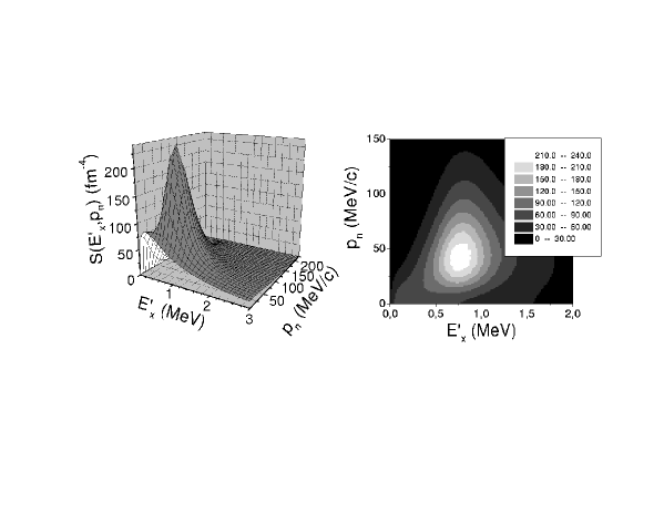
FIG. 4.: Spectral function (eq.(52)) after knockout of one of the halo neutrons in ⁶He by the electron. The figure in the right side is the contour plot of the spectral function shown in the left part.

VI Results

In this section we give the results for the observables derived in section IV for an electron scattering process on ⁶He. The computations are done following the steps given in section V.

All the observables can be computed in two different scenarios. First, assuming that the participant particle is one of the neutrons and the unbound ⁵He system survives in the final state; and second, the $\alpha$ particle is the one knocked out by the electron and the two neutrons survive undisturbed in the final state. In both cases we consider that we are in the corresponding quasielastic peak, i.e. the energy transfer is $\omega=q^{2}/2M$ where $M$ is the neutron mass in the first case and the ⁴He mass in the second case.

A Spectral functions and momentum distributions

The spectral function $S(E^{\prime}_{x},p_{3})$ is given in (52), while in (104) we show its analytic form obtained from the specific expressions used for the wave functions. As already mentioned, this function gives the probability of removing the participant particle with momentum $p_{3}$ leaving the residual system with energy $E^{\prime}_{x}$.

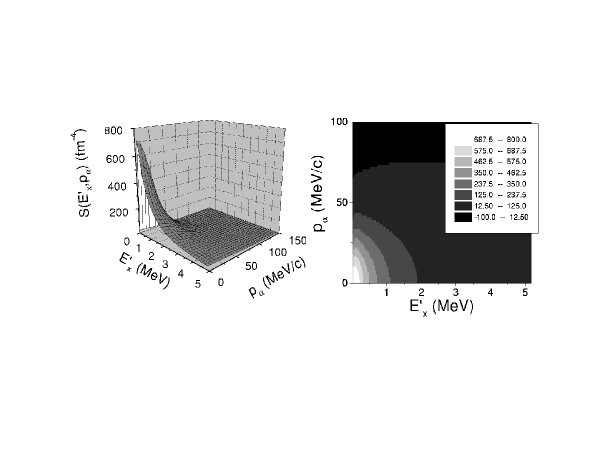
FIG. 5.: Same as fig.4 for the case of $\alpha$ knockout by the electron.

Let us start with the case of a participant neutron. The spectral function is shown in fig.4, and reflects the momentum distribution of the internal nucleon and the energy spectrum of the unbound system ⁵He. In the left part of the figure we show the spectral function itself, while the right part shows the projection over the basis.

The spectral function has a peak whose precise position is easily seen in the right part of the figure. The maximum value corresponds to a ⁵He energy of roughly $E^{\prime}_{x}=0.75$ MeV, that is the energy of the lowest $p_{3/2}$ resonance in ⁵He (0.77 MeV [42]). The width of this resonance is relatively small (less than 0.7 MeV), and this makes the peak clearly pronounced. The next resonance in ⁵He ($p_{1/2}$) has an energy of around 2 MeV, and it should also appear in the figure. However, its large width, more than 5 MeV, makes this resonance to be smeared out and hidden by the $p_{3/2}$. Furthermore, as mentioned in subsection V.D, more than 82% of the norm of the ⁶He wave function is given by the $p_{3/2}$ wave, while the $p_{1/2}$ only gives around 6%. The presence of $s$–waves in the ⁶He wave function ($\sim$ 10%) makes the spectral function non zero along the $p_{n}=0$ edge.

In fig.5 we show the same as in fig.4 but for the case where the $\alpha$–particle is scattered away by the electron, and the two neutrons act as spectators. In this case the overlap (96) is computed writing the ⁶He wave function in terms of the Jacobi coordinates with $x$ connecting both neutrons. From table I we know that both neutrons are preferably in a relative $s$–state, and this will produce a non zero spectral function along the $p_{\alpha}=0$ axis. The fact that the spectral function is proportional to $\sqrt{E^{\prime}_{x}}$ (see eq.(104)) will make the function equal to zero at the origin. This peaked spectral function close to the origin reflects the fact that the $n-n$ interaction has a very large scattering length for the ${}^{1}S_{0}$–wave (more than 23 fm), giving rise to a virtual state at very low energy (less than 100 keV).

FIG. 6.: (a) Neutron momentum distribution (see eq.(55)) for the participant neutron case. The contributions to the total from the $s_{1/2}$ wave (short–dashed), $p_{1/2}$ wave (dot–dashed), and $p_{3/2}$ wave (long–dashed) are shown. The inset shows the same contributions multiplied by $p_{n}^{2}$, where the weight of each wave can be better appreciated. (b) Same as (a) for the $\alpha$ momentum distribution in the participant $\alpha$ case.

After integration of the spectral function over the internal two–body energy $E^{\prime}_{x}$ we obtain the internal momentum distribution of the participant particle (eq.(55)). In fig.6a we show the computed neutron momentum distribution after integration over $E^{\prime}_{x}$ of the spectral function in fig.4 (solid line). The contributions to the total from the $s_{1/2}$ wave (short–dashed line), $p_{1/2}$ wave (dot–dashed line), and $p_{3/2}$ wave (long–dashed line) are also shown. It may look that the $s$–wave contribution is much larger than the 10% given in table I. This is because the whole contribution at the origin comes from the $s$ waves. However, when computing the normalization of the momentum distribution the phase volume contains a $p_{n}^{2}$ factor, that reduces the weight of the $s$ contribution. In the inset of fig.6a we show the neutron momentum distribution multiplied by $p_{n}^{2}$. We clearly see that dominant contribution comes from the $p_{3/2}$ wave, while the $s$ contribution is small.

In fig.6b we show the same but for the case of participant $\alpha$. Again the solid line shows the total $\alpha$ momentum distribution, and the long–dashed and short–dashed correspond to the contributions from the $s$ and $p$ waves, respectively. In this case (table I) the dominant term is the relative neutron–neutron state with orbital angular momentum zero. In fact the long–dashed curve and the solid one coincide almost in the whole range of $\alpha$ momenta. Even when the momentum distribution is multiplied by the $p_{\alpha}^{2}$ factor coming from the phase volume (inset in fig.6b) it is seen that the $s$ waves are the clearly dominant ones, and they are responsible for the pronounced peak observed in the spectral function in fig.5.

B Cross sections and response functions

To compute the cross sections (53) and (66) we work in the in plane perpendicular kinematics (see end of section IV). The momentum transfer $q$ is fixed at a value of $q=190$ MeV/c, and the energy transfer corresponds to the center of the quasielastic peaks ($\omega=q^{2}/2m_{3}$), with $m_{3}=m_{n}$ or $m_{3}=m_{\alpha}$. The cross sections (53) and (66) are then functions of the polar angles of the particle detected in coincidence with the electron, i.e. $\theta_{p^{\prime}_{3}}$ and $\theta_{p^{\prime}_{i}}$, respectively.

i) Participant neutron.

Let us first consider the case when $\omega$ corresponds to the center of the neutron quasielastic peak. As discussed at the end of section II only a halo neutron can be the participant particle. If the particle detected in coincidence with the electron is the participant neutron ($(e,e^{\prime}n)$ process) the cross section is given by eq.(53). Assuming that the internal energy $E^{\prime}_{x}$ can be neglected in eq.(44) the cross section can then also be written as shown in (57).

In fig.7 we show the differential cross section for this process. Two cases have been considered, one of them at a forward scattering angle ($\theta_{e}=30$), and the second one at a backward scattering angle ($\theta_{e}=150$). The electron beam energy $E_{0}$ takes a value of 375 MeV in the first case, and 108 MeV in the second. In the figure the solid line is the calculation as given in eq.(53). The dashed line is the calculation as in (57) where $E^{\prime}_{x}$ has been fully neglected in eq.(44), i.e. $E^{\prime}_{x}=0$. Finally the long dashed line is the calculation as in (57) but taking $E^{\prime}_{x}=0.77$ MeV in eq.(44). This energy corresponds to the energy of the lowest $p$–resonance in ⁵He.

FIG. 7.: Differential cross section for a $(e,e^{\prime}n)$ reaction for a participant neutron process. The participant neutron is assumed to be detected in coincidence with the electron. The calculations with scattering angles $\theta_{e}=30$ and $\theta_{e}=150$ are shown. The solid lines are calculations as given in (53). The short–dashed and long–dashed lines are calculations as given in (66) taking $E^{\prime}_{x}=0$ and $E^{\prime}_{x}=0.77$ MeV in (44), respectively. The inset shows the structure functions appearing in (53).

As seen in the figure the three computed cross sections are very similar, with only a small difference in the maximum, that is placed at a value of $\theta_{p^{\prime}_{n}}$ of roughly 10 degrees. When the approximation in (57) is used the chosen value for $E^{\prime}_{x}$ in eq.(44) is not very relevant, and only a full calculation as in (53) reduces the maximum and the value at $\theta_{p^{\prime}_{n}}=0$. In all cases the cross section is already negligible for outgoing neutrons with polar angle larger than 75 degrees.

The calculations with different scattering angles differ roughly in a global scale factor. This is because for a participant neutron only the magnetic nucleon form factor is important. Hence, in eq.(57) the main contribution is given by the transverse structure function, and the whole dependence on the scattering angle is contained in the global factor $\sigma_{M}V_{T}$. From eqs.(22) and (39) one sees that $\sigma_{M}V_{T}$ goes like $1/\sin^{2}(\theta_{e}/2)$ and scattering angles close to zero give a much larger contribution than scattering angles close to $\pi$. This is seen in fig.7, where the maximum value of the cross section is 8 times larger for $\theta_{e}=30$ than for $\theta_{e}=150$. In the inset in fig.7 we show the four response functions in eq.(57). It is clear that, as mentioned above, the dominant contribution is by far given by the transverse part. Only $W_{LT}$ gives an additional non negligible contribution.

When the participant particle is one of the halo neutrons, either the second halo neutron or the core can also be detected in coincidence with the electron. In this case the cross section is given by eq.(66), where $p^{\prime}_{i}$ is the momentum either of the spectator neutron or of the spectator core (eq.(63)). The solid lines in fig.8a give the differential cross section when the particle detected in coincidence with the electron is the second neutron. Therefore it also contributes to the $e^{\prime}n$ coincidence cross section. The two cases with $\theta_{e}=30$ (thick lines) and $\theta_{e}=150$ (thin lines) are shown. As seen in the figure, for both scattering angles the maximum contribution to the cross section appears at an angle of around 70 degrees, value for which the cross sections shown in fig.7 are already small. Furthermore for small angles the contribution to the $e^{\prime}n$ coincidence cross section coming from the spectator neutron is more than 10 times smaller than the contribution from the participant neutron (see fig.7). In fig.8b we show the total differential cross section (solid line) of the $e^{\prime}n$ coincidence reaction for $\theta_{e}=30$. This curve is obtained by summing up the contribution from the participant neutron (short–dashed line in fig.8b, or solid line for $\theta_{e}=30$ in fig.7) and the contribution from the spectator neutron (thick solid line in fig.8a). From fig.8b it is then clear that the behavior of the cross section is dominated by the participant neutron, while the spectator neutron contributes with a roughly constant cross section that creates a long tail that extends all the way up to $\theta_{p^{\prime}_{n}}=180$. When $\theta_{e}=150$ the difference is basically a global factor close to 8. We also show in fig.8a the differential cross section for the $e^{\prime}\alpha$ coincidence process when the $\alpha$ particle is a spectator. They are given by the dashed curves, and show a pronounced peak at 70 degrees.

FIG. 8.: (a) Differential cross sections for coincidence reactions after a participant neutron process and assuming that the particle detected in coincidence with the electron is either the spectator neutron (solid line) or the spectator $\alpha$ (dashed line). Calculations with $\theta_{e}=30$ (thick lines) and $\theta_{e}=150$ (think lines) are shown. (b) Total differential cross section after an electron–neutron coincidence reaction (solid line). The contributions from the participant neutron (short–dashed line) and the spectator neutron (long–dashed line) are shown. The dotted line is the differential cross section for a $(e,e^{\prime}\alpha)$ process assuming that the $\alpha$ is the participant particle.

ii) Participant $\alpha$.

Let us finish with the case when $\omega$ corresponds to the center of the $\alpha$ quasielastic peak. The participant particle is then the $\alpha$, $m_{3}=m_{\alpha}$, and for $q=190$ MeV/c the energy transfer is around 5 MeV. Neglecting $E^{\prime}_{x}$ in eq.(44), and taking $M_{h}=m_{1}+m_{2}+m_{3}$, it can be seen that the angle $\theta_{p^{\prime}_{3}}$ has to satisfy that $\sin\theta_{p^{\prime}_{3}}\leq(m_{1}+m_{2})/m_{3}$. This relation is fulfilled for any angle when the participant particle is one of the halo neutrons, but when $m_{3}>(m_{1}+m_{2})$ it gives a limit to the value of $\theta_{p^{\prime}_{3}}$. In particular, for a participant $\alpha$ particle one has that $\theta_{p^{\prime}_{3}}\lesssim 30$. This is also shown in fig.8b, where the dotted curve shows the differential cross section for an exclusive $(e,e^{\prime}\alpha)$ reaction in the center of the $\alpha$ quasielastic peak. The cross section is zero for angles larger than 30, and the maximum value at the origin is around twice the one obtained in the $e^{\prime}n$ coincidence process. In the computation shown in the figure the scattering angle is 30 degrees, for which $E_{0}=369$ MeV ($q=190$ MeV/c, $\omega=q^{2}/2m_{\alpha}$). As seen in eq.(40), only a longitudinal structure function enters in this case, and the whole dependence on the scattering angle is then contained in $\sigma_{M}$. Therefore different scattering angles only introduce a global factor determined by the ratio between the different values of the Mott cross section. For instance, a scattering angle of 15 degrees would make the differential cross section four times larger than the one shown in the figure, while $\theta_{e}=150$ would make the cross section more than 200 times smaller than the one in the figure. After $\alpha$ knockout by the electron the spectator neutrons could in principle be detected in coincidence with the outgoing electron. The computed cross section for this process is very small, and barely visible in the scale of fig.8b.

VII Summary and final remarks

The fact that electron scattering is one of the most powerful and cleanest procedures in order to investigate nuclear structure lead us to consider these reactions to investigate one of the most intriguing objects recently discovered in nuclear physics: Halo nuclei. In particular we have considered the case of two–neutron halo nuclei. The three–body wave function of the nucleus is obtained by solving the Faddeev equations in coordinate space by means of the adiabatic hyperspherical expansion. As soon as the two–body interactions between the constituents of the nucleus are specified the three–body structure can be computed to the needed accuracy.

First we have made a short incursion into elastic electron scattering reactions where we have seen the variation of the charge form factor according to two limiting values for the charge r.m.s. radius, the core size and the ⁶He size. The validity of the three–body picture requires that the charge form factor for ⁶He and ⁴He should be similar. In other words, if the present picture of ⁶He as a ⁴He core and two halo neutrons is correct, the elastic differential cross section for ⁶He should be practically identical to that of ⁴He, while if the spatial charge distribution of ⁶He would be as extended as that of the neutrons, the cross section would be at least four times smaller at typical $q$ values of 200 – 300 MeV/c. Thus elastic electron scattering provides a direct test of the halo picture.

Then we make an extensive discussion of $(e,e^{\prime}x)$ processes, that are described in the impulse approximation, i.e. the virtual photon is absorbed by a single constituent of the halo nucleus. The quasielastic exclusive electron scattering formalism was developed years ago (see for instance [33]), and in principle one could directly apply it to electron scattering on halo nuclei. However, the language used in the three–body description of the halo nucleus (inert core, Jacobi coordinates, …) is not easily matched with the language commonly used in electron scattering, where the single–particle properties of nuclei play an important role. One of the main aims of this paper has been to obtain the differential cross section for electron scattering using the three–body wave function of the halo nucleus as starting point. Comparison of the derived cross section with the well known expression for quasielastic exclusive electron scattering permits an easy identification of the observables of interest: Spectral function, response functions, and momentum distributions.

After discussion of the kinematics of the reaction we have applied the method to electron scattering on ⁶He, for which the two–body interactions between its three constituents are well known. These interactions reproduce the basic properties of the nucleus, separation energy and root mean square radius, together with an important amount of experimental data obtained after fragmentation on stable targets. Uncertainties coming from a poor description of the halo nucleus are then minimized. We have investigated the different observables for the cases of a participant neutron and a participant $\alpha$.

We have first studied the spectral function, that carries the whole information about the structure of the two–body subsystem obtained after removal by the electron of one of the constituents of ⁶He. This function is interpreted as the probability of removing one of the constituents with a certain momentum leaving the residual system with a certain energy. Effects due to the presence of different partial waves can be observed, as well as indications about the resonance structure of the surviving unbound two–body subsystem. Of special interest is the case of neutron removal, since the spectral function directly gives information about the unbound nucleus ⁵He.

After integration of the spectral function over the energy we obtain the momentum distribution of the participant particle, that contains information about the weight of each partial wave in the wave function. Experimental information about the momentum distribution can in principle be obtained by taking the ratio between the measured cross section and the electron–participant particle cross section. However, one has to keep in mind that the factorization of the five–differential cross section is only approximated, and low lying resonances in the final unbound two–body system are required. For the same reason as before, low lying resonances in the two–body system are necessary in order to write the five–differential cross section in terms of the response functions (that are simply the product of the momentum distribution and the corresponding single–particle response function). This can always be done when the residual nuclear system is bound. We have seen that for ⁵He (that has a resonance at an energy of around 0.8 MeV) the approximated differential cross section does not differ very much from the exact one, and it is therefore possible to talk about response functions in this kind of reactions. Such a response functions have been obtained for the case of a participant neutron, where the transverse response clearly dominates, and for a participant $\alpha$, where only the longitudinal one enters.

In summary, as for any nucleus, electron scattering is probably the most accurate procedure in order to investigate the structure of halo nuclei. Due to the up to now unattainable technical problems, experimental measurements are not available, and these reactions have been completely unexplored. Fortunately the first experiments of this kind are projected for the next few years [30], and theoretical studies as the ones presented here are then needed. We have derived the cross section and investigated for the case of the two–neutron halo nucleus ⁶He how the observables are connected to the structure of the nucleus. We show results for differential cross sections corresponding to elastic scattering as well as to quasielastic scattering on a neutron halo and on the ⁴He core, illustrating how the different kinematical regions probe the charge distribution, the spectral function and the momentum distributions in a transparent manner. Additional information could also be obtained exploiting spin polarization degrees of freedom, which are not discussed here given the incipient state of the subject.

A Derivation of the transition matrix

In fig.2 we show the scheme of the exclusive $(e,e^{\prime}x)$ reaction together with the notation for the different energies and momenta involved. The axis system chosen to describe the process is given in fig.1b. If we denote by $\mbox{\boldmath$r$}_{i}$ ($i=0,1,2,3$) the position of the electron and the three particles in the halo nucleus we then define the coordinates:

$$x = \mbox{\boldmath$r$}_{1}-\mbox{\boldmath$r$}_{2}$$ (A1)

$$y = \frac{m_{1}\mbox{\boldmath$r$}_{1}+m_{2}\mbox{\boldmath$r$}_{2}}{m_{1}+m_{2}}-\mbox{\boldmath$r$}_{3}$$ (A2)

$$z = \mbox{\boldmath$r$}_{0}-\mbox{\boldmath$r$}_{3}$$ (A3)

The coordinates $x$ and $y$ are the Jacobi coordinates except for the mass factors that are usually introduced and that for simplicity have been omitted here (see for instance [25]).

The conjugated momenta associated to the coordinates $x$, $y$, and $z$ are

$$\mbox{\boldmath$p$}_{x} = \frac{m_{2}}{m_{1}+m_{2}}\mbox{\boldmath$p$}_{1}-\frac{m_{1}}{m_{1}+m_{2}}\mbox{\boldmath$p$}_{2}$$ (A4)

$$\mbox{\boldmath$p$}_{y} = \frac{m_{3}}{m_{1}+m_{2}+m_{3}}(\mbox{\boldmath$p$}_{1}+\mbox{\boldmath$p$}_{2})-\frac{m_{1}+m_{2}}{m_{1}+m_{2}+m_{3}}\mbox{\boldmath$p$}_{3}$$ (A5)

$$\mbox{\boldmath$p$}_{z} = \frac{m_{3}}{m_{0}+m_{3}}\mbox{\boldmath$p$}_{0}-\frac{m_{0}}{m_{0}+m_{3}}\mbox{\boldmath$p$}_{3}$$ (A6)

and the same with primes in the final state. The masses of the three halo constituents are denoted by $m_{i}$ ($i=1,2,3$).

Working in the frame of the halo nucleus ($\mbox{\boldmath$p$}_{h}=\mbox{\boldmath$p$}_{1}+\mbox{\boldmath$p$}_{2}+\mbox{\boldmath$p$}_{3}=0$) one has

$$\mbox{\boldmath$p$}_{y}=\mbox{\boldmath$p$}_{1}+\mbox{\boldmath$p$}_{2}=-\mbox{\boldmath$p$}_{3}$$ (A7)

Following [44] in the one photon exchange approximation the transition matrix element for an electron scattering process is given by

$$S_{fi}=-ie\int dtd\mbox{\boldmath$r$}_{0}\bar{\psi}_{f}(t,\mbox{\boldmath$r$}_{0})\gamma_{\mu}\psi_{i}(t,\mbox{\boldmath$r$}_{0})A^{\mu}(t,\mbox{\boldmath$r$}_{0})$$ (A8)

where $\psi_{i,f}$ are the initial and final electron wave functions, that are given by

$$\psi_{i}(t,\mbox{\boldmath$r$}_{0})=\frac{1}{\sqrt{V}}u(\mbox{\boldmath$p$}_{0},\sigma_{0})e^{-iE_{0}t}e^{i\mbox{\boldmath$p$}_{0}\cdot\mbox{\boldmath$r$}_{0}}$$ (A9)

$$\psi_{f}(t,\mbox{\boldmath$r$}_{0})=\frac{1}{\sqrt{V}}u(\mbox{\boldmath$p$}^{\prime}_{0},\sigma^{\prime}_{0})e^{-iE_{0}^{\prime}t}e^{i\mbox{\boldmath$p$}_{0}^{\prime}\cdot\mbox{\boldmath$r$}_{0}}$$ (A10)

that are normalized to 1 in a volume $V$. $\sigma_{0}$ and $\sigma_{0}^{\prime}$ are the third components of the spin for the ingoing and outgoing electrons, respectively.

The four-vector $A^{\mu}(t,\mbox{\boldmath$r$}_{0})$ is the potential (scalar and vector) generated by the nucleus and seen by the electron at the instant $t$ in the position $\mbox{\boldmath$r$}_{0}$.

Substituting (A9) and (A10) into (A8) one has

$$S_{fi}=$$ (A12)

$$\frac{-ie}{V}\bar{u}(\mbox{\boldmath$p$}^{\prime}_{0},\sigma^{\prime}_{0})\gamma_{\mu}u(\mbox{\boldmath$p$}_{0},\sigma_{0})\int dtd\mbox{\boldmath$r$}_{0}e^{-i\omega t}e^{i\mbox{\boldmath$q$}\cdot\mbox{\boldmath$r$}_{0}}A^{\mu}(t,\mbox{\boldmath$r$}_{0})$$

Making use of the Maxwell equations one has

$$\Box A^{\mu}(t,\mbox{\boldmath$r_{0}$})=e\langle f|\hat{J}^{\mu}|i\rangle$$ (A13)

and the transition matrix element takes the form [35]

$$S_{fi} = \frac{-ie^{2}}{V}\bar{u}(\mbox{\boldmath$p$}^{\prime}_{0},\sigma^{\prime}_{0})\gamma_{\mu}u(\mbox{\boldmath$p$}_{0},\sigma_{0})$$ (A15)

$$\frac{1}{q_{\rho}^{2}}\int dtd\mbox{\boldmath$r$}_{0}e^{-i\omega t}e^{i\mbox{\boldmath$q$}\cdot\mbox{\boldmath$r$}_{0}}\langle f|\hat{J}^{\mu}|i\rangle$$

where $\hat{J}^{\mu}$ is the nuclear current operator ($\hat{J}^{\mu}=(\hat{\rho},\hat{\mbox{\boldmath$J$}})$).

The initial hadronic state $|i\rangle$ is given by the three–body halo wave function that is written as

$$\Psi^{JM}(\mbox{\boldmath$x$},\mbox{\boldmath$y$})\frac{1}{\sqrt{V}}e^{-iE_{h}t}e^{i\mbox{\boldmath$p$}_{h}\cdot\mbox{\boldmath$r$}_{h}}$$ (A16)

with

$$\mbox{\boldmath$r$}_{h}=\frac{m_{1}\mbox{\boldmath$r$}_{1}+m_{2}\mbox{\boldmath$r$}_{2}+m_{3}\mbox{\boldmath$r$}_{1}}{m_{1}+m_{2}+m_{3}}$$ (A17)

and $\Psi^{JM}(\mbox{\boldmath$x$},\mbox{\boldmath$y$})$ is the intrinsic three–body halo wave function with spin $J$ and third component $M$.

The wave function of the two–body system made by particles 1 and 2 in the final state is written as

$$\frac{1}{V}w^{s_{12},\sigma_{12}}(\mbox{\boldmath$p$}^{\prime}_{x},\mbox{\boldmath$x$})e^{-i(E^{\prime}_{1}+E^{\prime}_{2})t}e^{i(\mbox{\boldmath$p$}^{\prime}_{1}+\mbox{\boldmath$p$}^{\prime}_{2})\cdot\mbox{\boldmath$r$}_{12}}$$ (A18)

where $w^{s_{12},\sigma_{12}}(\mbox{\boldmath$p$}^{\prime}_{x},\mbox{\boldmath$x$})$ is the intrinsic continuum wave function, $s_{12}$ is the coupling of the spins of both particles and $\sigma_{12}$ its third component, and $\mbox{\boldmath$r$}_{12}=(m_{1}\mbox{\boldmath$r$}_{1}+m_{2}\mbox{\boldmath$r$}_{2})/(m_{1}+m_{2})$.

The final hadronic state $|f\rangle$ is made by the product of eq.(A18) and the plane wave describing the outgoing particle 3

$$\frac{1}{\sqrt{V}}e^{-iE^{\prime}_{3}t}e^{i\mbox{\boldmath$p$}^{\prime}_{3}\cdot\mbox{\boldmath$r$}_{3}}\chi_{s_{3},\sigma_{3}^{\prime}}$$ (A19)

where $\chi_{s_{3},\sigma_{3}^{\prime}}$ is the spin state of particle 3 in the final state.

According to the scheme shown in fig.2 particle 3 is the only constituent interacting with the electron. The rest of them are just spectators. The nuclear current operator should then be the one associated to the hadron labeled by 3. Assuming that this current operator depends only on the distance $z$ between particle 3 and the electron and substituting (A16), (A18), and (A19) into (A15) a little algebra leads to

$$S_{fi} = \frac{i}{V^{3}}\frac{e^{2}}{q_{\rho}^{2}}(2\pi)^{4}\delta(E_{i}-E_{f})\delta^{3}(\mbox{\boldmath$P$}_{i}-\mbox{\boldmath$P$}_{f})$$ (A23)

$$\bar{u}(\mbox{\boldmath$p$}^{\prime}_{0},\sigma^{\prime}_{0})\gamma_{\mu}u(\mbox{\boldmath$p$}_{0},\sigma_{0})$$

$$\sum_{\sigma_{3}}\int d\mbox{\boldmath$z$}e^{i\mbox{\boldmath$q$}\cdot\mbox{\boldmath$z$}}\langle\chi_{s_{3},\sigma_{3}^{\prime}}|\hat{J^{\mu}}(\mbox{\boldmath$z$})|\chi_{s_{3},\sigma_{3}}\rangle(2\pi)^{3}$$

$$\langle\frac{1}{(2\pi)^{3}}e^{i\mbox{\boldmath$p$}_{y}\cdot\mbox{\boldmath$y$}}\chi_{s_{3},\sigma_{3}}w^{s_{12},\sigma_{12}}(\mbox{\boldmath$x$},\mbox{\boldmath$p^{\prime}_{x}$})|\Psi^{JM}(\mbox{\boldmath$x$},\mbox{\boldmath$y$})\rangle$$

where we have used that $d\mbox{\boldmath$r$}_{0}d\mbox{\boldmath$r$}_{1}d\mbox{\boldmath$r$}_{2}d\mbox{\boldmath$r$}_{3}=d\mbox{\boldmath$r$}_{0}d\mbox{\boldmath$x$}d\mbox{\boldmath$y$}d\mbox{\boldmath$z$}$, and where the integrations over $t$ and $\mbox{\boldmath$r$}_{0}$ give rise to the deltas forcing energy and momentum conservation. $E_{i}=E_{0}+E_{h}$ and $E_{f}=E^{\prime}_{0}+E^{\prime}_{1}+E^{\prime}_{2}+E^{\prime}_{3}$ are the initial and final total energies, and analogously for the initial and final total momenta $\mbox{\boldmath$P$}_{i}$ and $\mbox{\boldmath$P$}_{f}$.

In deriving (A23) we have also used that particle 3 absorbs the whole energy and momentum transfer to the nucleus, and then in the frame of the three–body halo system one has

$$\mbox{\boldmath$p$}_{1}+\mbox{\boldmath$p$}_{2}=\mbox{\boldmath$p$}_{y}=-\mbox{\boldmath$p$}_{3}=\mbox{\boldmath$p$}^{\prime}_{1}+\mbox{\boldmath$p$}^{\prime}_{2}=\mbox{\boldmath$p$}^{\prime}_{y}$$ (A24)

Therefore in this picture the center of mass momentum of the final two–body system made by particles 1 and 2 reveals the internal momentum of the participant particle 3.

We denote now

$$J^{\mu}_{\sigma_{3}^{\prime},\sigma_{3}}(\mbox{\boldmath$q$},\mbox{\boldmath$p$}_{3})=\frac{1}{(2\pi)^{3/2}}\int d\mbox{\boldmath$z$}e^{i\mbox{\boldmath$q$}\cdot\mbox{\boldmath$z$}}\langle\chi_{s_{3},\sigma_{3}^{\prime}}|\hat{J^{\mu}}(\mbox{\boldmath$z$})|\chi_{s_{3},\sigma_{3}}\rangle$$ (A25)

that is the matrix element in momentum space of the current operator connecting states of particle 3 with spin projections $\sigma_{3}$ and $\sigma^{\prime}_{3}$.

We also define

$$M^{JM}_{s_{12}\sigma_{12},s_{3}\sigma_{3}}(\mbox{\boldmath$p$}^{\prime}_{x},\mbox{\boldmath$p$}^{\prime}_{y})=$$ (A27)

$$\langle\frac{1}{(2\pi)^{3}}e^{i\mbox{\boldmath$p$}^{\prime}_{y}\cdot\mbox{\boldmath$y$}}\chi_{s_{3},\sigma_{3}}w^{s_{12},\sigma_{12}}(\mbox{\boldmath$x$},\mbox{\boldmath$p^{\prime}_{x}$})|\Psi^{JM}(\mbox{\boldmath$x$},\mbox{\boldmath$y$})\rangle$$

that is the overlap between the initial three–body halo wave function and the wave function of the final two–body system (the exponential is the two–body center of mass motion). When the interaction between particles 1 and 2 is neglected the distorted function $w^{s_{12},\sigma_{12}}(\mbox{\boldmath$x$},\mbox{\boldmath$p^{\prime}_{x}$})$ becomes a plane wave ($e^{i\mbox{\boldmath$p^{\prime}_{x}$}\cdot\mbox{\boldmath$x$}}\chi_{s_{12},\sigma_{12}}$) and (A27) is the Fourier transform (normalized to 1) of the three-body halo wave function.

With (A25) and (A27) we can finally write the transition matrix element (A23) in the form

$$S_{fi} = \frac{i}{V^{3}}\frac{e^{2}}{q_{\rho}^{2}}(2\pi)^{17/2}\delta(E_{i}-E_{f})\delta^{3}(\mbox{\boldmath$P$}_{i}-\mbox{\boldmath$P$}_{f})$$ (A30)

$$\bar{u}(\mbox{\boldmath$p$}^{\prime}_{0},\sigma^{\prime}_{0})\gamma_{\mu}u(\mbox{\boldmath$p$}_{0},\sigma_{0})$$

$$\sum_{\sigma_{3}}J^{\mu}_{\sigma_{3}^{\prime},\sigma_{3}}(\mbox{\boldmath$q$},\mbox{\boldmath$p$}_{3})M^{JM}_{s_{12}\sigma_{12},s_{3}\sigma_{3}}(\mbox{\boldmath$p$}^{\prime}_{x},\mbox{\boldmath$p$}^{\prime}_{y})$$

B Electron-nucleon off–shell structure functions

For the off–shell electron-nucleon cross section we have chosen what in refs.[36, 38] is called prescription CC1 with current conservation.

Let us call

$$\alpha=F_{1}(q_{\mu}^{2})+F_{2}(q_{\mu}^{2});\hskip 42.67912pt\beta=\frac{-F_{2}(q_{\mu}^{2})}{2M_{\mbox{nucleon}}}$$ (B1)

The response functions defined as in eq.(39) are then (in plane kinematics is assumed)

$${\cal R}_{L} = \frac{1}{2E_{3}E_{3}^{\prime}}\left[\alpha^{2}(2E_{3}E_{3}^{\prime}+m_{3}^{2}-p_{3}^{\mu}p_{3\mu}^{\prime})+\right.$$ (B3)

$$\left.(E_{3}+E^{\prime}_{3})^{2}(\beta^{2}(m_{3}^{2}+p_{3}^{\mu}p_{3\mu}^{\prime})+2\alpha\beta m_{3})\right]$$

$${\cal R}_{T} = \frac{1}{E_{3}E_{3}^{\prime}}\left[\alpha^{2}(p^{\prime 2}_{3}\sin^{2}\theta_{p^{\prime}_{3}}-m_{3}^{2}+p_{3}^{\mu}p_{3\mu}^{\prime})+\right.$$ (B5)

$$\left.2p^{\prime 2}_{3}\sin^{2}\theta_{p^{\prime}_{3}}(\beta^{2}(m_{3}^{2}+p_{3}^{\mu}p_{3\mu}^{\prime})+2\alpha\beta m_{3})\right]$$

$${\cal R}_{LT} = -\frac{\sqrt{2}}{E_{3}E_{3}^{\prime}}p^{\prime}_{3}\sin\theta_{p^{\prime}_{3}}(E_{3}+E^{\prime}_{3})$$ (B7)

$$\left[\alpha^{2}+2\beta^{2}(m_{3}^{2}+p_{3}^{\mu}p_{3\mu}^{\prime})+4\alpha\beta m_{3}\right]$$

$${\cal R}_{TT} = -\frac{1}{E_{3}E_{3}^{\prime}}p^{\prime 2}_{3}\sin^{2}\theta_{p^{\prime}_{3}}$$ (B9)

$$\left[\alpha^{2}+2\beta^{2}(m_{3}^{2}+p_{3}^{\mu}p_{3\mu}^{\prime})+4\alpha\beta m_{3}\right]$$

Finally

$$F_{1}(q_{\mu}^{2})=\frac{G_{E}+\tau G_{M}}{1+\tau};\hskip 28.45274ptF_{2}(q_{\mu}^{2})=\frac{G_{M}-G_{E}}{1+\tau}$$ (B10)

where $\tau=-q_{\mu}^{2}/(4M_{\mbox{nucleon}})$, and $G_{E}$ and $G_{M}$ are parameterized as in [45].

REFERENCES

• [1] I. Tanihata, H. Hamagaki, O. Hashimoto, Y. Shida, N. Yoshikawa, K. Sugimoto, O. Yamakawa, T. Kobayashi, and N. Takahashi, Phys. Rev. Lett. 55 (1985) 2676.
• [2] I. Tanihata et al., Phys. Lett. B 160 (1985) 380.
• [3] T. Kobayashi, O. Yamakawa, K. Omata, K. Sugimoto, T. Shimoda, N. Takahashi, and I. Tanihata, Phys. Rev. Lett. 60 (1988) 2599.
• [4] I. Tanihata, Nucl. Phys. A 488 (1988) 113c.
• [5] P.G. Hansen and B. Jonson, Europhys. Lett. 4 (1998) 409.
• [6] Y. Tosaka and Y. Suzuki, Nucl. Phys. A 512 (1990) 46.
• [7] L. Johannsen, A.S. Jensen, and P.G. Hansen, Phys. Lett. B 244 (1990) 357.
• [8] M.V. Zhukov, B.V. Danilin, D.V. Fedorov, J.S. Vaagen, F.A. Gareev, and J.M. Bang, Phys. Lett. B 26 (1991) 19.
• [9] M.V. Zhukov, D.V. Fedorov, B.V. Danilin, J.S. Vaagen, and J.M. Bang, Nucl. Phys. A 529 (1991) 53.
• [10] K. Riisager, A.S. Jensen, and P. Møller, Nucl. Phys. A 548 (1992) 393.
• [11] P.G. Hansen, A.S. Jensen, and B. Jonson, Ann. Rev. Nucl. Part. Sci., 45 (1995) 591.
• [12] M.V. Zhukov, B.V. Danilin, D.V. Fedorov, J.M. Bang, I.J. Thompson, and J.S. Vaagen, Phys. Rep. 231 (1993) 151.
• [13] R. Anne et al., Phys. Lett. B 250 (1990) 19.
• [14] N.A. Orr et al., Phys. Rev. Lett. 69 (1992) 2050.
• [15] N.A. Orr et al., Phys. Rev. C 51 (1995) 3116.
• [16] M. Zinser et al., Phys. Rev. Lett. 75 (1995) 1719.
• [17] T. Nilsson et al., Europhys. Lett. 30 (1995) 19.
• [18] F. Humbert et al., Phys. Lett. B 347 (1995) 198.
• [19] M. Zinser et al., Nucl. Phys. A 619 (1997) 151.
• [20] M.V. Zhukov, L.V. Chulkov, D.V. Fedorov, B.V. Danilin, J.M. Bang, J.S. Vaagen, and I.J. Thompson, J. Phys. G 20 (1994) 201.
• [21] A.A. Korsheninnikov and T. Kobayashi, Nucl. Phys. A 567 (1994) 97.
• [22] M.V. Zhukov and B. Jonson, Nucl. Phys. A 589 (1995) 1.
• [23] F. Barranco, E. Vigezzi, and R.A. Broglia, Phys. Lett. B 319 (1993) 387.
• [24] E. Garrido, D.V. Fedorov, and A.S. Jensen, Phys. Rev. C 53 (1996) 3159.
• [25] E. Garrido, D.V. Fedorov, and A.S. Jensen, Phys. Rev. C 55 (1997) 1327.
• [26] E. Garrido, D.V. Fedorov, and A.S. Jensen, Nucl. Phys. A 617 (1997) 153.
• [27] E. Garrido, D.V. Fedorov, and A.S. Jensen, Europhys. Lett. 43 (1998) 386.
• [28] J.D. Walecka, Theoretical Nuclear and Subnuclear Physics, Oxford University Press, (1995).
• [29] J.J. Kelly, Adv. Nucl. Phys. 23 (1996) 77.
• [30] T. Ohkawa and T. Katayama, Proc. of the Particle Accelerator Conference, Vancouver (1997) 30.
• [31] T, de Forest, Jr. and J.D. Walecka, Adv. in Phys. 15 (1966) 1.
• [32] H. de Vries, C.W. de Jager, and C. de Vries, At. Dat. and Nucl. Dat. Tab. 36 (1987) 495.
• [33] S. Frullani and J. Mougey, Adv. Nucl. Phys. 14 (1984) 1.
• [34] S. Boffi, C. Giusti, and F.D. Pacati, Phys. Rep. 226 (1993) 1.
• [35] T.W. Donnelly and J.D. Walecka, Ann. Rev. Nucl. Sci. 25 (1975) 329.
• [36] T. de Forest, Jr., Nucl. Phys. A 392 (1983) 232.
• [37] A.S. Raskin and T.W. Donnelly, Ann. of Phys. 191 (1989) 78.
• [38] J.A. Caballero, T.W. Donnelly, and G.I. Poulis, Nucl. Phys. A 555 (1993) 709.
• [39] D.V. Fedorov, A.S. Jensen, and K. Riisager, Phys. Rev. C 49 (1994) 201.
• [40] A. Cobis, D.V. Fedorov, and A.S. Jensen, J. Phys. G 23 (1997) 401.
• [41] A. Cobis, D.V. Fedorov, and A.S. Jensen, Phys. Rev. Lett. 79 (1997) 2411.
• [42] F. Ajzenberg–Selove, Nucl. Phys. A 490 (1988) 1.
• [43] B.V. Danilin, M.V. Zhukov, J.S. Vaagen, and J.M. Bang, Phys. Lett. B 302 (1993) 129.
• [44] J.D. Bjorken and S.D. Drell, Relativistic Quantum Mechanics, McGraw Hill (1964) pp. 100.
• [45] S. Galster et al., Nucl. Phys. B 32 (1971) 221.