Abstract

The validity of the approximations done in the mean field description of the quasi-elastic excitation of medium-heavy nuclei is discussed. A test of the reliability of the plane wave Born approximation is presented. The uncertainty related to the choice of the electromagnetic nucleon form factors is discussed. The effects produced by the meson exchange currents generated by the exchange of a single pion are studied, as well as the need of including relativistic corrections to the one-body currents. The results of the continuum shell model and those of the Fermi gas model are compared and the need of treating the emitted nucleon within a relativistic framework is studied. We analyze the results of Random Phase Approximation calculations not only in terms of their effects on the mean field responses, but also in terms of the theoretical consistency in the choice of the effective residual interaction. The role of the final state interaction is investigated. A microscopic justification of the use of complex optical potential to describe the final state interaction is provided. The effects of the final state interaction on the mean field responses are studied with a sum rule conserving model. A comparison with the experimental data measured in the ¹²C and ⁴⁰Ca nuclei is shown.

1 Introduction

The Mean Field (MF) model is the basis of any description of many-particle systems. In this model the particles composing the system are supposed to move independently from each other in an average potential. Under this assumption the complicated many-body problem is transformed into a set of, easy to solve, one-body problems. The solution of the MF equations produces a set of orthonormal single particle (sp) states whose tensor product forms a basis in the many-body Hilbert space. This basis is used in more complicated many-body treatments.

Usually the behavior of the real many-particle systems is quite different from the MF predictions. There are however phenomena which can be rather well described by the MF model. In these cases the more complicated many-body effects can be treated as a correction to the MF solution. One of these phenomena is the quasi-elastic (QE) excitation which is dominated by the single particle dynamics, well described by the MF approach in terms of one-particle one-hole (1p-1h) excitations.

Experimentally, the QE excitation is obtained by using probes which interact weakly with the system and by controlling the kinematical conditions in such a way that only one of the particles composing the system is directly struck by the external probe. This produces a relatively small perturbation of the system which however responds as a whole because the knocked particle is linked to the other ones. The total response is related to the characteristics of the interaction among the particles.

In the electron excitation of the atomic nuclei, the region where the nuclear response is quasi-elastic is well identified. The inelastic electron scattering cross section shows an evident peak at higher energies than those of the giant resonance region. The position of this peak is located at values very close to $|{\bf q}|^{2}/2M$, where ${\bf q}$ is the momentum transferred from the electron to the nucleus and $M$ is the nucleon mass. The width of the peak increases when the mass number of the target nucleus increases. These two facts lead to the interpretation of the peak as produced by the elastic scattering of the electron with a single nucleon. An ideal experiment on a free nucleon produces a narrow peak positioned exactly at $|{\bf q}|^{2}/2M$. Understanding the deviation from this situation means understanding the nuclear electron excitation mechanism and the nuclear many-body dynamics.

Figure 1: FG model results compared with the experimental data of refs. [Yat93, Wil97] for the ⁴⁰Ca nucleus. The electron energies $\varepsilon$ and the scattering angles $\theta$ are indicated in the figures. The dashed lines show the results obtained by using the values of $k_{\rm F}$=251 MeV/$c$ and $\langle E\rangle$=28 MeV fixed in ref. [Mon71]. The full lines have been calculated changing the values of the Fermi momentum and of the average binding energy to reproduce at best the experimental data: (a) $k_{\rm F}$=340 MeV/$c$ and $\langle E\rangle$=0 MeV, (b) $k_{\rm F}$=330 MeV/$c$ and $\langle E\rangle$=5 MeV, (c) $k_{\rm F}$=330 MeV/$c$ and $\langle E\rangle$=5 MeV and (d) $k_{\rm F}$=320 MeV/$c$ and $\langle E\rangle$=90 MeV.

The first electron scattering experiment aimed to probe the nuclear QE response was done at the Stanford Mark III linear accelerator in the early seventies [Mon71]. The data were analyzed within a Fermi gas (FG) model [Mon69], i.e. considering the nucleus as an infinite system of non interaction fermions, and the corresponding fits were obtained by changing the two parameters of the model: the average nucleon interaction energy, $\langle E\rangle$, and the Fermi momentum, $k_{\rm F}$. The position of the peak is fixed by $\langle E\rangle$, while both height and width are determined by the Fermi momentum. The interesting result was that the three quantities could be reproduced so well by two parameters.

The aim of this experiment work was to obtain an empirical estimate of the value of $k_{\rm F}$. The commonly accepted value of $k_{\rm F}$ (about 270 MeV/$c$) is obtained from the empirical value of nuclear matter density, $\rho=0.17$ fm^-3, fixed by considering the nucleus a homogeneous sphere of radius $R=r_{0}A^{\frac{1}{3}}$, with $r_{0}=1.18$ fm given by elastic electron scattering experiments. The fit procedure used to reproduce the QE data provided for heavy nuclei a roughly constant value of $k_{\rm F}$ of about 260 MeV/$c$, in good agreement with the value obtained with the usual procedure.

The success of this description of the data within a FG model suppressed interest in the investigation of the QE peak for about ten years, until the data of the separated charge and current responses became available [Alt80]. The FG model which successfully explained the cross section was unable to describe separately its two components [Alt80].

Looking back at the analysis of the pioneering Stanford experiment we find that what is nowadays considered interesting physics is hidden in the two parameters of the fit. The nuclear structure problem and the interplay between single-particle and many-body dynamics have been obscured by the fit procedure.

In fig. 1 we compare the FG results with the recent ⁴⁰Ca data taken at Bates [Yat93, Wil97]. The values of $\langle E\rangle$ and $k_{\rm F}$ defined in ref. [Mon71] produce cross sections well above the data (see dashed curves). On the other hand, if $\langle E\rangle$ and $k_{\rm F}$ are fixed to reproduce one data set (full lines) the other ones are not well described.

The FG model provides a qualitative description of the phenomenon, but to obtain a quantitative description of the different sets of data it is necessary to go beyond this model and treat explicitly those degrees of freedom that are hidden in the effective values of the two parameters of the model.

The aim of this article is to discuss the successes and failures of the MF description of the electron induced QE excitation of medium and heavy nuclei. The discussion will be focused on what can be learnt about the interaction between the electromagnetic probe and the nucleus and the dynamics of the nuclear excitation. In the presentation we shall try to separate the problems concerning the reaction mechanism from those regarding the nuclear structure. This separation is somewhat artificial but it is useful to better determine and clarify the various approximations and uncertainties done in the study of the QE peak.

The description of the reaction mechanism is based upon the Plane Wave Born Approximation and the use of the traditional electromagnetic one-body operators, and we shall discuss the limits of all these approximations considering the distortion of the electron wave functions, the presence of Meson Exchange Currents and the relativistic corrections to the one-body operators.

The nuclear structure problem is tackled within the non-relativistic formalism. The basic model we shall adopt is the Continuum Shell Model, where the nucleons move independently from each other in a finite size average potential. We shall present, however, results obtained by describing the nucleus as an infinite system of non interacting nucleons. In addition to these MF descriptions of the excitation we shall also discuss results obtained with the Random Phase Approximation theory.

2 The electron-nucleus interaction

Our understanding of the electromagnetic processes is certainly deeper than that of those processes dominated by the strong interaction. There are however various problems not very well solved, or defined, in the description of the interaction between electrons and nuclei. In this section we shall discuss some of them. We shall present first what we call the standard derivation of the inelastic electron nucleus cross section. Then we shall discuss the validity of the approximations done in this approach, with special attention to their influence on the study of the QE excitation. In particular, the role of the nucleon form factors, the relativistic corrections and the Meson Exchange Currents are discussed.

2.1 The standard treatment

In this section we present the basic points of the usual derivation of the electron scattering cross section off atomic nuclei. More detailed presentations of this derivation can be found in various review articles (see, e.g., [deF66, Don75, Cio80, Dre89, Bof96]).

Throughout the paper we shall use the Bjorken and Drell [Bjo64] metric and the convention that the repeated indexes of a four-vector imply a sum on them: $a_{\mu}b^{\mu}=a_{0}b^{0}-{\bf a\cdot b}$.

Using the standard Feynman rules, the scattering amplitude for a single photon exchange process can be written as [Bjo64]:

$$\langle f,k_{f}|S|i,k_{i}\rangle\,=\,-i\int{\rm d}^{4}x\,[e{\overline{\psi}}_{f}(x)\gamma_{\mu}A^{\mu}(x)\psi_{i}(x)]\,.$$ (1)

In this equation the initial (final) state of the system is defined as the tensor product between the initial (final) state of the electron and of the nucleus. As we work in the Plane Wave Born Approximation (PWBA), the electron wave functions are plane wave solution of the free Dirac equation:

$$\psi(x)\,=\,\sqrt{\frac{m}{\varepsilon V}}\,u(k,s)\,e^{-ik^{\mu}x_{\mu}}\,.$$ (2)

where $u$ is one of the positive energy four-component Dirac spinors [Bjo64]. The electron states are characterized by the values of the four-momentum $k\equiv\{\varepsilon,{\bf k}\}$. The final formulae will be independent of the normalization volume $V$.

In eq. (1) we have indicated with $A^{\mu}$ the classical electromagnetic field generated by the nucleus. This should satisfy the field equation:

$$\Box A^{\mu}(x)\,=\,e\langle f|J^{\mu}(x)|i\rangle\,,$$ (3)

where $\Box\equiv\nabla^{2}-\partial^{2}/\partial t^{2}$ and $J^{\mu}$ is the nuclear current operator. The calculation now proceed by inserting the solution of eq. (3) and the expression of the electron wave functions (2) in eq. (1) which can be rewritten as:

$$\langle f,k_{f}|S|i,k_{i}\rangle\,=\,-ie^{2}\langle k_{f}|j_{\mu}|k_{i}\rangle\frac{g^{\mu\nu}}{q^{\beta}q_{\beta}}\int{\rm d}^{4}x\,e^{-iq_{\alpha}x^{\alpha}}\langle f|J_{\nu}(x)|i\rangle\,,$$ (4)

where the four-momentum transfer is defined as $q^{\nu}=k^{\nu}_{i}-k^{\nu}_{f}$ and the electron current is given by:

$$\langle k_{f}|j_{\mu}|k_{i}\rangle\,=\,\frac{m}{V}\sqrt{\frac{1}{\varepsilon_{i}\varepsilon_{f}}}\,{\overline{u}}(k_{f},s_{f})\,\gamma_{\mu}\,u(k_{i},s_{i})\,.$$ (5)

The nuclear current is supposed to be described by an operator local in ${\bf r}$. Its time dependence is given by:

$$J_{\mu}(t,{\bf r})\,=\,e^{iHt}\,J_{\mu}({\bf r})\,e^{-iHt}\,.$$ (6)

After performing the integration on the time variable the scattering amplitude can be expressed as:

$$\langle f,k_{f}|S|i,k_{i}\rangle\,=\,-ie^{2}\,2\pi\,\delta(E_{i}-E_{f}-\omega)\,\langle k_{f}|j_{\mu}|k_{i}\rangle\,\frac{1}{q^{\nu}q_{\nu}}\,\langle f|J^{\mu}({\bf q})|i\rangle\,,$$ (7)

where the $E_{i}$ and $E_{f}$ indicate, respectively, the initial and final energy of the nucleus and $\omega$ is the energy transferred by the electron. The expression (7) depends explicitly on the Fourier transform of the nuclear current

$$J_{\mu}({\bf q})\,=\,\int{\rm d}^{3}x\,e^{i{\bf q\cdot r}}\,J_{\mu}({\bf r})\,.$$ (8)

The nuclear current should satisfy the continuity equation:

$$\partial_{\mu}J^{\mu}(x)=0\,,$$ (9)

which, using the explicit time dependent expression (6), can be written, in coordinate space, as :

$$\nabla\cdot{\bf J}({\bf r})\,=\,-i\omega J^{0}({\bf r})$$ (10)

while in momentum space it assumes the form:

$${\bf q}\cdot{\bf J}({\bf q})\,=\,\omega\,\rho({\bf q})\,,$$ (11)

where we have used $J^{0}\equiv\rho$. The continuity equation imposes a relation between the four components of the nuclear current, therefore only three of them are independent. It is necessary to choose the independent components to be used to express the scattering amplitude. It is convenient to work in a reference system where the quantization $z$-axis points along the direction of the momentum transfer ${\bf q}$. Eq. (11) shows that the component of the current along this axis, the longitudinal component $J_{z}$, can be expressed in terms of the charge operator $\rho$. Therefore the scattering amplitude can be expressed in terms of $\rho$ and of two components orthogonals to the direction of ${\bf q}$. These are called transverse components and they are usually expressed in spherical coordinates:

$${\bf J}_{\pm}=\mp\frac{1}{\sqrt{2}}\left({\bf J}_{x}\pm i{\bf J}_{y}\right)\,.$$ (12)

To calculate the cross section one has to square the scattering amplitude, to average on the initial states and to sum over the final ones. Since the electron energies $\varepsilon$ are much bigger than its rest mass $m$, it is common to use the so called ultrarelativistic approximation consisting in neglecting the terms depending on $m$. The calculation is rather long but it can be done without any further approximation. The cross section assumes the expression:

$$\frac{{\rm d}^{2}\sigma}{{\rm d}\Omega{\rm d}\varepsilon_{f}}\,=\,\sigma_{\rm Mott}\,\left\{\left(\frac{q^{\mu}q_{\mu}}{q^{2}}\right)^{2}R_{L}(q,\omega)+\left(\tan^{2}\frac{\theta}{2}-\frac{q^{\mu}q_{\mu}}{2q^{2}}\right)R_{T}(q,\omega)\right\}\,,$$ (13)

where $\theta$ is the scattering angle, defined as the angle between the directions of ${\bf q}$ and ${\bf k}_{f}$, $q=|{\bf q}|$ and $\sigma_{\rm Mott}$ is the Mott cross section

$$\sigma_{\rm Mott}\,=\,\left(\frac{\alpha\cos(\theta/2)}{2\varepsilon_{i}\sin^{2}(\theta/2)}\right)^{2}\,,$$ (14)

where we have indicated with $\alpha$ the fine structure constant.

In the expression (13) the cross section is composed of two parts, each of them formed by a kinematical term and a response function containing the full nuclear structure information. The longitudinal and transverse response functions are respectively defined as:

$$R_{L}(q,\omega) = \overline{\sum_{i}}\sum_{f}\delta(E_{f}-E_{i}-\omega)|\langle f|\rho(q)|i\rangle|^{2}$$ (15)

$$R_{T}(q,\omega) = \overline{\sum_{i}}\sum_{f}\delta(E_{f}-E_{i}-\omega)\left(|\langle f|J_{+}(q)|i\rangle|^{2}\,+\,|\langle f|J_{-}(q)|i\rangle|^{2}\right)\,.$$ (16)

The bar on the sum on $i$ indicates the average on the initial states.

If the expression (13) of the cross section is valid it is possible to obtain an experimental separation of the longitudinal and transverse responses. To achieve this goal it is necessary to perform a set of measurements at fixed $\omega$ and $q$ but for different values of the scattering angle $\theta$. The ratio of the cross section and $\sigma_{\rm Mott}$ should be plotted against $v_{T}=\tan^{2}(\theta/2)-(\omega^{2}-q^{2})/(2q^{2})$ and all the points should lie on a straight line. The slope of this line gives $R_{T}$ while the intersection with the $y$ axis provides $R_{L}$. This procedure is called the Rosenbluth separation [Ros50].

The nuclear responses are calculated under the hypothesis that the nucleus makes a transition from one state of definite angular momentum $|i\rangle\equiv|J_{i}M_{i}\rangle$ to another one $|f\rangle\equiv|J_{f}M_{f}\rangle$. For this reason it is convenient to rewrite eq. (8) by making a multipole expansion of the exponential. Considering the parity of the nuclear final state, it is possible to separate the electric and magnetic transitions and at the end one has to deal with three type of multipole operators: the Coulomb operators producing transitions of natural parity,

$$M_{JM}(q)\,=\,\int{\rm d}^{3}r\,j_{J}(qr)\,Y_{JM}(\hat{r})\,\rho({\bf r})\,,$$ (17)

the electric current operators which give rise also to transitions of natural parity,

$$T^{\rm E}_{JM}(q)\,=\,\frac{1}{q}\int{\rm d}^{3}r\,\left\{\nabla\times\left[j_{J}(qr){\bf Y}^{M}_{JJ}(\hat{r})\right]\right\}\cdot{\bf J}({\bf r})\,,$$ (18)

and the magnetic current operators producing transitions of unnatural parity,

$$T^{\rm M}_{JM}(q)\,=\,\int{\rm d}^{3}r\,j_{J}(qr)\,{\bf Y}^{M}_{JJ}(\Omega)\cdot{\bf J}({\bf r})\,.$$ (19)

In the eqs. (17)-(19) $j_{J}$ indicates a spherical Bessel function, $Y_{JM}$ is a spherical harmonics and ${\bf Y}^{M}_{JL}$ is a vector spherical harmonics [Edm57].

We shall deal with scattering from doubly closed shell nuclei, therefore $J_{i}=0$ and then the value of the angular momentum of the final state correspond to the multipolarity of the transition. The nuclear responses can be written as:

$$R_{L}(q,\omega) = 4\pi\sum_{\beta}\sum^{\infty}_{J=0}\,|\langle\beta,J\parallel M_{J}(q)\parallel 0\rangle|^{2}\,\delta(E_{\beta}-\omega)\,,$$ (20)

$$R_{T}(q,\omega) = 4\pi\sum_{\beta}\sum^{\infty}_{J=1}\,\left(|\langle\beta,J\parallel T^{\rm E}_{J}(q)\parallel 0\rangle|^{2}+\right.$$ (21)

$$\left.\hskip 56.9055pt|\langle\beta,J\parallel T^{\rm M}_{J}(q)\parallel 0\rangle|^{2}\right)\,\delta(E_{\beta}-\omega)\,,$$

where $\beta$ indicates all the quantum numbers characterizing the nuclear final state other than $J$.

The only elements which remain to be specified are the explicit expressions of the nuclear electromagnetic operators $\rho$ and ${\bf J}$. Up to now the only hypothesis made on these operators has been done in eq. (6). Since in general the nuclear many-body wave functions are described using nucleonic degrees of freedom in a non relativistic framework, the standard treatment considers the electromagnetic operators produced by non relativistic pointlike nucleons. This means that the nuclear charge is composed by the charge of the nucleons and the current is composed by the movement of the charged nucleons inside the nucleus (convection current) and by the sum of the magnetic currents associated with the nucleons spin (magnetization current). The expressions of these operators are:

$$\rho({\bf r})\,=\,\sum^{A}_{k=1}\frac{1+\tau^{3}_{k}}{2}\,\delta({\bf r}-{\bf r}_{k})\,,$$ (22)

for the charge operator,

$${\bf j}^{\rm C}({\bf r})\,=\,\sum^{A}_{k=1}\frac{-i}{2M_{k}}\,\frac{1+\tau^{3}_{k}}{2}\,\left[\delta({\bf r}-{\bf r}_{k})\nabla_{k}+\nabla_{k}\delta({\bf r}-{\bf r}_{k})\right]\,,$$ (23)

for the convection current operator, and

$${\bf j}^{\rm M}({\bf r})\,=\,\sum^{A}_{k=1}\frac{1}{2M_{k}}\,\left(\mu^{\rm P}\frac{1+\tau^{3}_{k}}{2}+\mu^{\rm N}\frac{1-\tau^{3}_{k}}{2}\right)\nabla\times\delta({\bf r}-{\bf r}_{k})\,\mbox{\boldmath$\sigma$}_{k}\,,$$ (24)

for the magnetization current operator. In the previous equations $M_{k}$ indicates the rest mass of $k$-th nucleon, $\mu^{\rm P}$ and $\mu^{\rm N}$ are the anomalous magnetic moment of the proton and the neutron respectively, $\mbox{\boldmath$\sigma$}_{k}$ is the Pauli spin matrix of the $k$-th nucleon and $\tau^{3}_{k}=1$ or -1 according the $k$-th nucleon to be a proton or a neutron.

The expressions (22), (23) and (24) of the one-body nuclear charge and current are obtained as Fourier transform of a specific non relativistic reduction of a nucleon current of the type:

$$J^{\mu}(P_{f}S_{f},P_{i}S_{i})\,=\,\overline{u}(P_{f},S_{f})\,\gamma^{\mu}\,u(P_{i},S_{i})\,,$$ (25)

where the $u$ are the nucleon Dirac spinors and $P$ and $S$ are respectively the four momentum and the spin of the nucleon. The procedure leading to the expressions (22)-(24) consists in retaining the zero and first order terms of an expansion in powers of $q^{\nu}=P^{\nu}_{f}-P^{\nu}_{i}$.

2.2 Coulomb distortion

The possibility of making an experimental separation of the longitudinal and transverse response functions is very appealing because it allows one to investigate separately the electron nucleus interaction and the nuclear excitation mechanism. The same nuclear model should be used to describe both responses, the only difference between them is due to the electromagnetic operator.

Figure 2: Rosenbluth plot for ¹²C(e,e’)¹²C and ⁴⁰Ca(e,e’)⁴⁰Ca reactions at the fixed excitation energy $\omega=300$ MeV. We have indicated with $\sigma_{M}$ the Mott cross section. Note that the DWBA points are not perfectly aligned.

We have seen that the Rosenbluth separation is possible if the expression (13) of the cross section is valid. In this expression the kinematics is well separated from the nuclear structure since the PWBA has been used, in other words, since it has been assumed that the electron wave functions are plane wave solutions of the Dirac equation. In this approach the effects of the electromagnetic field of the nucleus on the motion of the electron are neglected. The validity of this approximation is quite good for few body systems or light nuclei, but it starts to become questionable already for nuclei as heavy as ¹²C [deF66, Cio80, Hei83].

It is possible to solve the Dirac equation for an electron moving in a static Coulomb potential [Yen54]. This provides the exact solution for the elastic scattering cross section. The situation is more difficult to handle in the case of inelastic scattering since the electromagnetic field generated by the nucleus is not any more static because it is produced by a transition from the ground to the excited state. In the most sophisticated treatment developed up to now, the one-photon exchange scattering amplitude (1) is calculated using the electron wave functions obtained by solving the Dirac equation with a Coulomb potential generated by the target nucleus ground state. This treatment is called Distorted Wave Born Approximation (DWBA) and its validity in the description of low lying states has been widely studied [Hei83].

There are two major effects that the DWBA adds to the PWBA description. The first is produced by the attraction between the positively charged nucleus and the negatively charged electron. The asymptotically measured initial and final momenta $k_{i}$ and $k_{f}$ are smaller than the effective momenta of the electron around the nucleus. This is an interpretation of the phenomenon based upon a PWBA description of the process, since DWBA wave functions are not eigenstates of the momentum operator of the electron. In this simplified picture the incoming electron is accelerated by the nucleus while the scattered electron is decelerated. This produces a transferred momentum larger than that of the PWBA. An empirical expression of the effective momentum transfer is obtained in the eikonal approximation [Hei83]:

$$q_{\rm eff}\,=\,q\left(1+1.5\frac{Z\alpha\hbar c}{\varepsilon_{i}R_{\rm eq}}\right)$$ (26)

with $R_{\rm eq}=1.24\,A^{1/3}$. The difference between the PWBA momentum transfer and the effective one increases with the charge $Z$ of the target nucleus and diminishes when the electron energy $\varepsilon_{i}$ increases.

The second DWBA effect is of quantum mechanical nature and consists in the focusing of the electron wave function onto the nucleus causing an increase of the flux and an enhancement of the cross section. This effect is partially compensated by the reduction of the cross section due to the $q_{\rm eff}$ shift.

In the DWBA expression of the cross section it is not possible to separate the nuclear from the electron variables. Furthermore there are interference terms between longitudinal and transverse amplitudes. In a Rosenbluth plot the DWBA cross sections do not lie on a straight line. If the distortion effects are small, however, it is possible to correct the experimental cross sections in order to have PWBA equivalent cross sections and to use them to make the Rosenbluth separation.

Distortion effects on the QE excitation have been studied for ¹²C and ⁴⁰Ca nuclei in ref. [Co’87a], where a full DWBA calculation has been done, and for ⁴⁰Ca and ²⁰⁸Pb nuclei in ref. [Tra88, Tra93], where an analytical expansion of the amplitudes up to $(Z\alpha)^{2}$ has been used.

A first finding of these studies is that the DWBA cross sections without corrections are rather well aligned on a Rosenbluth plot. Within the experimental uncertainty their alignment is compatible with an exact straight line (see fig. 2). For this reason the alignment of the cross sections on a Rosenbluth plot cannot be considered a proof of the validity of PWBA.

The major effect of the distortion on a Rosenbluth plot consists in a rotation of the line around the intersection point with the $y$ axis. This does not modify very much the value of the longitudinal response but it has a rather big effect on the value of the transverse response function. These considerations are valid for a fixed value of the excitation energy.

In ref. [Tra88] the full energy dependence of the responses has been studied. The distortion effects on ⁴⁰Ca consists mainly of a shift to higher energies and it can be rather well described in terms of $q_{\rm eff}$. The situation in ²⁰⁸Pb is more complicated since the focusing of the wave function plays an important role.

The effects of the distortion are small enough to be considered a correction to the PWBA, therefore it is reasonable to extract the responses from the cross section using the procedure outlined above.

2.3 Nucleon electromagnetic form factors

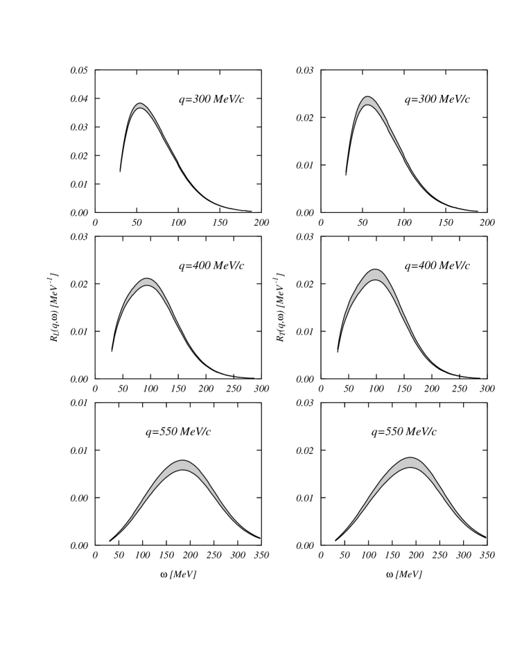
Figure 3: ¹²C response functions. The bands show the uncertainty related to the choice of the the nucleon electromagnetic form factors.

In the standard derivation, the nuclear current has been obtained under the assumption of pointlike nucleons. In the QE excitation the values of the energies and momenta involved are such that the nucleon internal structure plays a noticeable role. This fact is taken into account by inserting nucleon electromagnetic form factors in the expression of the current. For a nucleon of type $\tau$ (either proton or neutron) with mass $M$, eq. (25) becomes:

$$J^{\mu}_{\tau}(P_{f}S_{f},P_{i}S_{i})\,=\,\overline{u}(P_{f},S_{f})\left[F^{\tau}_{1}(q^{2})\gamma^{\mu}+i\kappa^{\tau}\frac{F^{\tau}_{2}(q^{2})}{2M}\sigma^{\mu\nu}q_{\nu}\right]u(P_{i},S_{i})$$ (27)

where

$$\sigma^{\mu\nu}=\frac{i}{2}(\gamma^{\mu}\gamma^{\nu}-\gamma^{\nu}\gamma^{\mu})$$ (28)

and $\kappa^{\tau}$ is set equal to the anomalous part of the magnetic moment in units of nucleon magnetons (1.79 for proton and -1.91 for neutron). The terms $F^{\tau}_{1}$ and $F^{\tau}_{2}$ are the Dirac form factors and they are normalized such as:

$$F^{p}_{1}(0)=1\,\,\,\, \,\,\,\,F^{p}_{2}(0)=1$$ (29)

$$F^{n}_{1}(0)=0\,\,\,\, \,\,\,\,F^{n}_{2}(0)=1\,.$$ (30)

For a more direct comparison with the experiment it is convenient to use the Sachs form factors related to the Dirac ones by the expressions:

$$G^{\tau}_{\rm E} = F^{\tau}_{1}+\kappa^{\tau}\frac{q_{\nu}q^{\nu}}{4M^{2}}F^{\tau}_{2}$$ (31)

$$G^{\tau}_{\rm M} = F^{\tau}_{1}+\kappa^{\tau}F^{\tau}_{2}\,.$$ (32)

The effect of the nucleon finite size is implemented by means of a convolution of the pointlike currents (22)-(24) with these nucleon form factors. Then, it is more convenient to work in $q$ space where the nucleon form factors are simply multiplicative factors.

The problem is now to find a functional dependence of the form factor in terms of $q$ and $\omega$ which is able to reproduce the elastic electron-nucleon data. Unfortunately the data are not selective enough to define a unique parameterization of this functional dependence. Different type of form factors can reproduce the elastic scattering data with the same degree of accuracy.

The sensitivity of the nuclear responses to the different choices of the electromagnetic nucleon form factors has been studied in ref. [Ama93b]. In that article we performed calculations of the QE responses with the same nuclear structure input but considering the nucleon form factors of refs. [Jan66, Ber72, Iac73, Hoe76, Sim80]. We found that the momentum and energy domain of the QE peak lies in a region of strong variations of the nucleon electromagnetic form factors, and the changes of the nuclear responses can be as big as 12% at the peak values (see fig. 3).

Some of the parametrizations we have used are old and have been ruled out by more modern measurements. Probably the 12% uncertainty we have quoted slightly overestimates the actual uncertainty on the form factor. In any case the study quoted above points out the need of specifying the nucleon form factor used when one compares the results of QE calculations with the experimental data. The ambiguities in the choice of the nucleon form factors set an intrinsic uncertainty threshold of the theoretical calculations.

2.4 Relativistic corrections

We have already said that the expressions of the one-body operators (22)-(24) are obtained by expanding the relativistic operator (25) in powers of $q$, $\omega$ and $P$, and retaining the zero and first order terms.

In ref. [Voy62] it has been pointed out that a consistent treatment of both the charge and the current operators, up to the same order in the expansion, produces a correction factor for the charge operator. This factor is called the Darwin-Foldy term

$$f_{\rm DF}\,=\,\left(1+\frac{q^{2}-\omega^{2}}{4M^{2}}\right)^{-1/2}$$ (33)

and it multiplies the electric Sachs form factor in the calculation of $R_{L}$. This correction reduces the longitudinal response as is shown in fig. 4.

Figure 4: The lines in this figure have all been obtained using the non relativistic FG model. The dashed lines present the result obtained by using the usual non relativistic one-body operators. The dotted curves include the Darwin-Foldy term (only in the longitudinal response). The full lines have been obtained considering the relativistic corrections to the operators.

A new non relativistic expansion of the on-shell electromagnetic one-body current has been proposed in ref. [Ama96a] for use in the region of the QE peak at high $q$ values. The idea of this approach is to obtain expressions of the current operators which are not truncated in powers of $q$ and $\omega$ and hence applicable at high values of energy and momentum transfer.

In a FG model the value of the momentum of a bound nucleon is at most of the order of the Fermi momentum $P\sim k_{\rm F}$. Therefore for a typical value of $k_{\rm F}=250$ MeV/$c$ we have $P/M\leq 1/4$ and hence an expansion of the current in powers of $P/M$ is justified.

The details of the calculation can be found in refs. [Ama96a, Ama96b, Jes98] and the final expressions of the charge and transverse current operators up to first order in $P/M$ are:

$$\rho({\bf q},\omega) = \frac{q}{\sqrt{q^{2}-\omega^{2}}}\,G_{\rm E}+i\,\frac{\left(G_{\rm M}-\frac{1}{2}G_{\rm E}\right)}{M\sqrt{4M^{2}+q^{2}-\omega^{2}}}({\bf q}\times{\bf P})\cdot\mbox{\boldmath$\sigma$}\,,$$ (34)

$${\bf J}^{T}({\bf q},\omega) = \frac{\sqrt{q^{2}-\omega^{2}}}{q}\left\{i\frac{G_{\rm M}}{2M}(\mbox{\boldmath$\sigma$}\times{\bf q})+\frac{G_{\rm E}}{M}\left({\bf P}-\frac{{\bf q}\cdot{\bf P}}{q^{2}}{\bf q}\right)\right\}\,.$$ (35)

The first piece of the charge operator is the usual non relativistic contribution $G_{\rm E}$ multiplied by a factor larger than one. This factor produces (see fig. 4) an increase of the non relativistic result which goes in the opposite direction with respect to the traditional Darwin-Foldy correction, and it can be directly implemented as a multiplicative factor in the non-relativistic models of the reaction. The second piece is the charge of the spin-orbit operator, which is slightly different from the one arising in the usual expansions. Finally, the transverse current operator contains the two traditional pieces, the magnetization and convection current operators, but both are corrected by a multiplicative factor smaller than one.

The results presented in fig. 4 show big relativistic effects at momentum transfer larger than 500 MeV/$c$. In these situations the value of the momentum of the emitted nucleon is comparable with its rest mass $M$, therefore a relativistic treatment of the motion of the emitted nucleon is necessary. This involves the nuclear structure part of the problem and we shall discuss this point more in detail in section 3.2.

2.5 Two-body currents

We have treated the problem of the electron excitation considering the nuclear current produced only by individual nucleons. This limitation is inconsistent already at the level of the standard derivation. Inserting the expression (6) into the continuity equation (9) one obtains:

$$\nabla\cdot{\bf J}({\bf r})\,=\,-i\left[H,\rho\right]\,=\,-i\left[T+V,\rho\right]\,,$$ (36)

where $T$ is the kinetic energy and $V$ the interaction term.

It can be shown that by using the expressions (22) and (23) for the charge and convection current operators the equation

$$\nabla\cdot{\bf j}^{\rm C}({\bf r})\,=\,-i\left[T,\rho\right]$$ (37)

is satisfied. It is obvious that a new term must be added to the one-body current in order to verify the continuity equation with the full hamiltonian. This new term, ${\bf J}^{\rm TB}$, must satisfy the equation

$$\nabla\cdot{\bf J}^{\rm TB}({\bf r})\,=\,-i\left[V,\rho\right]$$ (38)

and it is a two-body operator.

The continuity equation shows the theoretical needs for including two-body currents, but it does not define them in an unique way, because all the operators which are divergenceless, for example the one-body magnetization current (24), are not restricted by this equation.

Since there is not a unique way to derive these two-body current operators, different approaches have been proposed in the literature. In any case, it is commonly accepted that the most important terms are those related to the exchange of mesons and more specifically to the exchange of a single pion.

We have calculated the contribution of the Meson Exchange Currents (MEC) following the approach of refs. [Gar76, Fri77, Van81]. Using the Feynman rules we have evaluated the contributions of the three diagrams of fig. 5 which we call seagull (a), pionic (b) and $\Delta$-isobar (c) terms.

Figure 5: Feynman diagrams of the three MEC operators we consider: (a) seagull, (b) pionic and (c) $\Delta$-isobar.

For the evaluation of the MEC terms we need a model for the pion-nucleon, photon-nucleon-$\Delta$ and pion-nucleon-$\Delta$ interactions. The models of the pion-nucleon interaction commonly used (pseudo-scalar and pseudo-vector couplings) produce the same result in the non-relativistic limit.

We define a function $h({\bf r})$ as the Fourier transform of the dynamical pion propagator

$$h({\bf r}-{\bf r}_{l})=\int\frac{{\rm d}^{3}k}{(2\pi)^{3}}\,\frac{F_{\pi\rm N}(k,\varepsilon)\,{\rm e}^{i{\bf k}\cdot({\bf r}-{\bf r}_{l})}}{k^{2}+m_{\pi}^{2}-\varepsilon^{2}}\,,$$ (39)

where we have indicated with $F_{\pi\rm N}$ the pion-nucleon form factor and with $\varepsilon=(\Delta E)_{l}$ the energy of the exchanged pion obtained as the difference between the energies of the final and initial single states of the $l$-th nucleon.

In momentum space we express the seagull and pionic currents respectively as:

$${\bf j}^{\rm S}({\bf q},\omega)=4\pi\frac{f_{\pi}^{2}}{m_{\pi}^{2}}\,F_{\rm S}(q,\omega)\sum_{k,l=1\atop k\neq l}^{A}\,[\mbox{\boldmath$\tau$}_{k}\times\mbox{\boldmath$\tau$}_{l}]_{{}_{3}}\,{\rm e}^{i{\bf q}\cdot{\bf r}_{k}}\mbox{\boldmath$\sigma$}_{k}\,\mbox{\boldmath$\sigma$}_{l}\cdot\nabla_{k}h({\bf r}_{k}-{\bf r}_{l})$$ (40)

and

$${\bf j}^{\pi}({\bf q},\omega) = -4\pi\frac{f_{\pi}^{2}}{m_{\pi}^{2}}\,F_{\pi}(q,\omega)\,\sum_{k,l=1\atop k\neq l}^{A}\,[\mbox{\boldmath$\tau$}_{k}\times\mbox{\boldmath$\tau$}_{l}]_{3}\,\,\int{\rm d}^{3}r\,{\rm e}^{i{\bf q}\cdot{\bf r}}\,$$ (41)

$$\mbox{\boldmath$\sigma$}_{k}\cdot\nabla h({\bf r}-{\bf r}_{k})\,\nabla\left[\mbox{\boldmath$\sigma$}_{l}\cdot\nabla h({\bf r-r}_{l})\right]\,.$$

The situation for the $\Delta$-isobar current is not so well defined because formulations based upon static quark models [Che71, Hoc73, Loc75, Ris79] or chiral lagrangian [Pec69, Van81, Alb90] give different expressions. We have adopted the point of view of the first group of authors and use the following expression:

$${\bf j}^{\Delta}({\bf q},r) = -iC_{\Delta}F_{\Delta}(q,\omega)\sum_{k,l=1\atop k\neq l}^{A}\,{\rm e}^{i{\bf q}\cdot{\bf r}_{k}}{\bf q}$$

$$\times\displaystyle\left\{[\mbox{\boldmath$\tau$}_{k}\times\mbox{\boldmath$\tau$}_{l}]_{3}\,\,\mbox{\boldmath$\sigma$}_{k}\times\nabla_{k}\mbox{\boldmath$\sigma$}_{l}\cdot\nabla_{k}h({\bf r}_{k}-{\bf r}_{l})\,-\,4\tau^{3}_{l}\nabla_{k}\mbox{\boldmath$\sigma$}_{l}\cdot\nabla_{k}h({\bf r}_{k}-{\bf r}_{l})\right\}\,.$$

In the above equations $f_{\pi}=0.079$ is the effective pion-nucleon coupling constant, $m_{\pi}$ is the pion mass and

$$C_{\Delta}=4\pi\frac{f_{\pi}^{2}}{m_{\pi}^{2}}\frac{4}{25M(M_{\Delta}-M)}\,,$$ (42)

with $M_{\Delta}$ the $\Delta$ mass. Finally, $F_{\rm S}$, $F_{\pi}$, $F_{\Delta}$ show the dependence on the electromagnetic nucleon, delta and pion form factors. As we have already discussed there are theoretical ambiguities in the choice of these form factors. In table 1 we show the effect of these ambiguities on the values of the peak of the MEC responses [Ama93a]. For the seagull current, the possible functional dependence of the $F_{\rm S}$ form factor, generate an appreciable uncertainty at the peak energy. For $q=550$ MeV/$c$, the uncertainty on the maximum is $\simeq 40\%$ of its value. A similar situation is found for the electromagnetic pion form factor $F_{\pi}$ included in the pionic current even if the uncertainty is considerably smaller than in the seagull case. Table 1 shows for example that, at $q=550$ MeV/$c$, the uncertainty of the peak value is $\sim 12\%$.

$q$ [MeV/$c$]	$\omega$ [MeV]	$\Delta F_{S}$ [%]	$\Delta F_{\pi}$ [%]
300	50	15.7	5.3
400	90	25.6	8.3
500	100	40.2	12.3

Table 1: Percentile uncertainty on the value of the peak of the response produced by the different choices of form factors on seagull and pionic currents [Ama93a].

For consistency with the one-body currents, we use in our calculations the following expressions for $F_{\rm S}$ and $F_{\pi}$:

$$F_{\rm S} = G_{\rm E}^{\rm P}-G_{\rm E}^{\rm N},$$ (43)

$$F_{\pi} = F_{\pi\gamma}=\frac{1}{1+(q^{2}-\omega^{2})/m_{\rho}^{2}}\,,$$ (44)

where $m_{\rho}$ is the mass of the $\rho$-meson.

The situation is even more complicated for the $\Delta$ current since the electromagnetic form factor $F_{\Delta}$ and the constant $C_{\Delta}$ are model dependent. The major uncertainty is related to $C_{\Delta}$, but a discussion of this problem is beyond the aim of the present work. The expression (42) of $C_{\Delta}$ we have chosen is widely used in the literature [Hoc73, Ris79, Ris84, Sch89]. For the form factor $F_{\Delta}$, following the static quark model, we use:

$$F_{\Delta}=2G_{\rm M}^{V}=G_{\rm M}^{\rm P}-G_{\rm M}^{\rm N}\,.$$ (45)

Finally, we would like to comment on the pion-nucleon form factor

$$F_{\pi\rm N}(k,\varepsilon)=\frac{\Lambda^{2}-m_{\pi}^{2}}{\Lambda^{2}+k^{2}-\varepsilon^{2}}$$ (46)

present in the pion propagator of eq. (39). We have verified [Ama93a, Ama93b] that, in the QE peak region, for the values of $\Lambda$ commonly accepted ($\sim 1$ GeV), the results are very close to those obtained considering simply $F_{\pi\rm N}=1$, which is the value we have adopted.

The MEC we have presented above act only on the transverse response. In principle MEC contributions are present also in the longitudinal response, but it has been shown [Lal97] that their effects are very small, of the order of 3% at the energy of the peak. For this reason in the following we shall neglect the corrections to the longitudinal response and we shall discuss only the effect of MEC on the transverse one.

The MEC are two-body operators, therefore they can produce the excitation of 1p-1h or 2p-2h pairs. In the excitation of 1p-1h pairs, the transition amplitudes of MEC and those of one-body currents interfere. These interference terms produce the larger contribution of the MEC to the 1p-1h response.

Figure 6: 1p-1h MEC contributions to the excitation of the ⁴⁰Ca transverse response at $q$=550 MeV/$c$. The full line shows the interference term between one-body current and MEC. The dashed line represents the pure MEC contribution.

Figure 7: 1p-1h transverse responses of ⁴⁰Ca. The dashed-dotted lines are the one-body responses. The remaining lines show the results obtained by adding the various parts of MEC: seagull (dashed-doubly-dotted), pionic (dashed), $\Delta$ isobar (dotted), seagull+pionic+$\Delta$ isobar (solid).

In fig. 6 we show the contribution of the MEC to the transverse response of ⁴⁰Ca for $q$=550 MeV/$c$. While the contributions of pure MEC are positive for all excitation energies, the contribution of the interference term between one-body current and MEC is positive at small energies and become negative at energies above 80 MeV.

Figure 8: 2p-2h responses of ¹²C for $q=550$ MeV/$c$. Panel (a): Seagull plus pionic contributions. The dashed line is the term corresponding to the two particle emission while the dotted line has been obtained for the case of one particle in the continuum and the other one on an excited bound state. The full curve represents the total 2p-2h response. Panel (b): Two nucleon emission contributions induced by the $\Delta$ isobar current. The dashed-dotted line corresponds to the emission of a proton-neutron pair. The dotted and dashed lines give the contribution of the two-proton and two-neutron emission, respectively, and are overlapping in the scale of the figure. The solid line is the total response.

Figure 9: Transverse responses calculated in ¹²C and ⁴⁰Ca. The solid lines represent the total responses including 1p-1h and 2p-2h final states. The dotted lines give the one-body response and the dashed lines the 2p-2h contributions. The dashed-dotted lines have been obtained with one-body operators only.

In agreement with [Koh81] we find that the effect of the pionic and seagull currents on the responses have opposite sign. The pionic current diminishes the pure one-body response, while the seagull increases it. In fig. 7 we show this fact for the ⁴⁰Ca nucleus, but we found analogous results also for the ¹²C response [Ama93a]. Considering only seagull and pionic currents we obtain an increase of the transverse response in the peak region [Ama92, Ama93b]. The inclusion of the $\Delta$ isobar current gives a negative contribution. The final results consists in a lowering of the one-body responses. The effect of the seagull and pionic currents becomes smaller as $q$ increases while that of the $\Delta$ isobar current remains roughly constant. For this reason, the total lowering effect of the MEC increases its magnitude with $q$.

In all the nuclear models we have used to calculate the response, the nuclear 1p-1h final states are orthogonal to the 2p-2h final states. This means that in our approach there is not interference between 1p-1h and 2p-2h excitation amplitudes and, as a consequence, the 2p-2h responses add to the 1p-1h ones.

The two body MEC operators can lead to different kinds of 2p-2h final states. A first classification concerns the number of particles which are in the continuum. A first type of 2p-2h state is produced when none of the two particles is in the continuum. These are low energy excitation and they do not contribute in the QE region. A second kind of excited state is formed when one particle is in the continuum and the other one is lying on a bound single particle state. Finally the last type of excited 2p-2h state is the one which has both particles in the continuum.

In the panel (a) of fig. 8 we show the behavior of the 2p-2h responses for the various types of final states. In this calculation only the seagull and pionic currents have been used. The contribution of the response where only one particle is in the continuum rapidly reaches a plateau value and it remains roughly constant with the increase of the excitation energy. Since the number of particle-hole configurations entering in the excitation of this part of the response remains constant even if the energy increases. The two-nucleon emission contribution behaves quite differently: its value increases steadily with the value of the excitation energy. This is related to the enlarging of the phase space available for the final states of this reaction.

The other possible classification of 2p-2h final states is related to the kind of particles which are emitted. Seagull and pionic currents are generated by the exchange of charged pions. The $\Delta$ isobar current is active also when a neutral pion is exchanged. Then, while the seagull and pionic currents can lead to final 2p-2h states where only a proton and a neutron pair is emitted, the $\Delta$ isobar current can emit also a pair of like nucleons.

The contribution of these different kind of excited states on the 2p-2h response of the $\Delta$ isobar current is shown in panel (b) of fig. 8. The two-proton and two-neutron emission responses are indistinguishable at the scale of the figure. This is due to the fact that ¹²C nucleus is practically symmetric in terms of proton-neutron single-particle structure. The number of protons and neutrons is the same, and the small differences in the single-particle energies and in the wave functions affect very little the response. The dominant emission channel remains the proton-neutron one, and its relative contribution becomes more important with increasing energies.

In fig. 9 we present the total QE transverse responses for ¹²C and ⁴⁰Ca. The 2p-2h responses are rather small below the peak but become important at higher energies.

A detailed analysis of the MEC contribution [Ama94a] shows that the pionic and seagull currents produce an increase of the values of the responses in the peak. The inclusion of the $\Delta$ isobar current has an opposite effect. If for $q$=300 MeV/$c$ the total responses are similar to the one-body responses, for higher values of $q$ they are even smaller. There is not big difference between the two nuclei, though in ⁴⁰Ca the modifications are slightly bigger. The greater effect we found is less than 5%, certainly within the range of uncertainty related to the choice of the nucleon and mesons form factors.

3 The nuclear excitation

In this section we shall present some of the models commonly used to describe the nuclear QE excitation. In this region the excitation energy of the nucleus is well above the continuum threshold, therefore at least one particle is emitted from the nucleus. Due to the relatively high values of energy and momentum transfer the QE excitation is not of collective type like vibrations or rotations, but the process is dominated by the single particle dynamics. The MF model is the obvious starting point of any description of this excitation. We shall first present the basic ideas of the MF model and in subsequent subsections we shall discuss the validity of the approximations made in this treatment.

3.1 Mean field models

In the MF model the many-body nuclear states are Slater determinants of sp wave functions. In the ground state all the sp states below the Fermi level are occupied and all the states above it are empty. The excited states of the system are generated by promoting nucleons from below to above the Fermi level. These basic ideas of the MF approach can be used with different set of sp bases, and this differentiate the various MF models. In our presentation we shall treat the shell model where the sp basis is generated considering the finite size of the nucleus and the FG model where the system is considered to be infinite and translationally invariant.

3.1.1 The Continuum Shell Model

The basis commonly used to describe finite nuclear systems is composed of sp states characterized by the orbital angular momentum $l$, the total angular momentum $j$, its projection $m$ on the $z$ axis and the isospin $z$ axis projection, $t$. For discrete sp states it is also necessary to specify the principal quantum number $n$,

$$|nljmt\rangle\equiv\psi^{t}_{nljm}({\bf r})\equiv R^{t}_{nlj}(r)\,{\cal Y}_{ljm}(\hat{r})\,\chi_{t}\,$$ (47)

where

$${\cal Y}_{ljm}(\hat{r})\,=\,\sum_{\mu s}\,\langle l\mu\frac{1}{2}s|jm\rangle\,Y_{l\mu}(\hat{r})\,\chi_{s}\,.$$ (48)

Here $\langle l\mu\frac{1}{2}s|jm\rangle$ is a Clebsh-Gordan coefficient, $\chi_{s}$ is the spin function, with $s$ the spin $z$ axis projection, and $\chi_{t}$ is the isospin function. For continuum sp states their energy $\epsilon$ must be given

$$|\epsilon ljmt\rangle\equiv\psi^{t}_{ljm}({\bf r},\epsilon)\equiv R^{t}_{lj}(r,\epsilon)\,{\cal Y}_{ljm}\,\chi_{t}\,.$$ (49)

One possibility of generating the set of sp states is to use a Hartree-Fock procedure as is done in ref. [Koh83]. This implies the choice of an effective nucleon-nucleon interaction and the solution of a system of non linear Schrödinger-like differential equations.

We use a different approach called Continuum Shell Model (CSM). We fix a central real potential $V(r)$ acting on all the nucleons, and we generate the sp states (47) and (49) by solving the traditional radial sp Schrödinger equation with the appropriate boundary conditions on the radial parts. The solutions of this equation should be regular at the origin. At high $r$ values bound states have exponential decay, while continuum states have oscillating behavior.

Figure 10: Sensitivity of the responses to the choice of the single particle wave functions. Full lines represent the results obtained with the Woods-Saxon set of refs. [Co’84, Co’85, Co’87b]. Dashed lines correspond to a new parameterization aiming to reproduce the charge density distributions. Thick full lines represents the empirical charge density distributions reconstructed using the Fourier-Bessel parameters given in ref. [DeJ87].

As we deal with one- and two-body operators, the only possible final states are of 1p-1h and 2p-2h types, with the particles in the continuum, which in this model are, respectively, given by:

$$|\beta,JM_{J}\rangle\,=\,|(\epsilon_{p}l_{p}j_{p}),(n_{h}l_{h}j_{h});JM_{J}\rangle\,,$$ (50)

$$|\beta,JM_{J}\rangle\,=\,|\left[(\epsilon_{p_{1}}l_{p_{1}}j_{p_{1}}),(\epsilon_{p_{1}}l_{p_{2}}j_{p_{2}});J_{p}\right],\left[(n_{h_{1}}l_{h_{1}}j_{h_{1}}),(n_{h_{1}}l_{h_{2}}j_{h_{2}});J_{h}\right];JM_{J}\rangle\,.$$ (51)

In the case of one-body operators, only the 1p-1h final states can be excited. The sum over $(\beta J)$ in eqs. (20) and (21) goes on all the possible 1p-1h configurations allowed by the angular momentum and parity composition rules. This means that $|j_{p}-j_{h}|\leq J\leq j_{p}+j_{h}$ and $(-1)^{l_{p}+l_{h}}$ should be equal to the parity of the corresponding electromagnetic transition. The transition amplitudes can be written as:

$$\langle\beta,J\parallel O^{\rm OB}_{J}(q)\parallel 0\rangle\,=\,\langle\epsilon_{p}l_{p}j_{p}\parallel O^{OB}_{J}(q)\parallel n_{h}l_{h}j_{h}\rangle\,\delta(\omega-\epsilon_{p}+\epsilon_{h})\,.$$ (52)

In case of two-body operators the expressions are slightly more complicated, and it is possible to excite both 1p-1h and 2p-2h final states. In the first case the same angular momentum, parity and energy rules as before apply and the transition amplitudes can be written as:

$$\langle\beta,J\parallel O^{\rm TB}_{J}(q)\parallel 0\rangle\,=\,\sum_{\alpha<\epsilon_{F}}\,\sum_{J_{1}J_{2}}\,(-1)^{J_{1}+J_{2}+J+1}\,\sqrt{(2J_{1}+1)(2J_{2}+1)}\,\left\{\begin{array}[]{ccc}J_{1}&J_{2}&J\\ j_{h}&j_{p}&j_{\alpha}\end{array}\right\}$$

$$\left[\,\langle(n_{\alpha}l_{\alpha}j_{\alpha}),(\epsilon_{p}l_{p}j_{p});J_{1}\parallel O^{\rm TB}_{J}(q)\parallel(n_{h}l_{h}j_{h}),(n_{\alpha}l_{\alpha}j_{\alpha});J_{2}\rangle\,+\right.$$

$$\hskip 2.84544pt\left.(-1)^{j_{\alpha}+j_{h}+J_{2}+1}\,\langle(n_{\alpha}l_{\alpha}j_{\alpha}),(\epsilon_{p}l_{p}j_{p});J_{1}\parallel O^{\rm TB}_{J}(q)\parallel(n_{\alpha}l_{\alpha}j_{\alpha}),(n_{h}l_{h}j_{h});J_{2}\rangle\,\right]\,$$

$$\delta(\omega-\epsilon_{p}+\epsilon_{h})\,,$$ (53)

where we have used a 6j coefficient.

If the final state has two particles in the continuum the transition amplitude is:

$$\langle\beta,J\parallel O^{\rm TB}_{J}(q)\parallel 0\rangle\,=\,(-1)^{j_{p_{1}}+j_{p_{2}}+J_{p}}\,\delta(\omega-\epsilon_{p_{1}}-\epsilon_{p_{2}}+\epsilon_{h_{1}}+\epsilon_{h_{2}})$$

$$\left[\,\langle(\epsilon_{p_{2}}l_{p_{2}}j_{p_{2}}),(\epsilon_{p_{1}}l_{p_{1}}j_{p_{1}});J_{p}\parallel O^{\rm TB}_{J}(q)\parallel(n_{h_{1}}l_{h_{1}}j_{h_{1}}),(n_{h_{2}}l_{h_{2}}j_{h_{2}});J_{h}\rangle\,+\right.$$ (54)

$$\left.(-1)^{j_{h_{1}}+j_{h_{2}}+J_{h}+1}\,\langle(\epsilon_{p_{2}}l_{p_{2}}j_{p_{2}}),(\epsilon_{p_{1}}l_{p_{1}}j_{p_{1}});J_{p}\parallel O^{\rm TB}_{J}(q)\parallel(n_{h_{2}}l_{h_{2}}j_{h_{2}}),(n_{h_{1}}l_{h_{1}}j_{h_{1}});J_{h}\rangle\,\right]\,,$$

where now $|J_{p}-J_{h}|\leq J\leq J_{p}+J_{h}$.

The above expressions show that in the MF model, the complicated problem of evaluating many-body transition matrix elements has been reduced to the much simple problem of calculating sums of one- and two-body transition matrix elements. The calculation of the sp transition matrix elements is long and tedious, but it does not present fundamental difficulties and it can be carried on without any further hypothesis or approximation. The explicit expressions of the matrix elements can be found in ref. [Ama93a].

We have studied the sensitivity of the CSM results to the choice of the potential parameters [Ama93a, Ama93b], the only input of the model. We have performed CSM calculations with two sets of parameters. The first one taken from the literature has been fixed to reproduce the sp energies around the Fermi level and it has been used to describe low-lying and giant resonance excitations [Co’84, Co’85, Co’87b]. The second set of parameters has been fixed to have good description of the empirical charge density distribution [Ama93a, Ama93b]. The comparison of the results obtained for one-body responses is shown in fig. 10. The difference between the results obtained with the two parametrizations becomes smaller at high values of $q$ and $\omega$. This indicates that in the QE peak the surface effects are not important. The differences between the two results are compatible with the uncertainty related to the choice of the nucleon form factors. All the CSM results we shall present have been obtained with the set of parameters of refs. [Co’84, Co’85, Co’87b].

3.1.2 Fermi gas model

An alternative MF model often used [Czy63, Mon69, Koh81, Van81, Bou91, Gar92, Gil97] to describe the QE excitation is the FG model. In this model the nucleus is treated as an infinite system of non-interacting fermions. Both the volume $\Omega$ of the system and number of particles $A$ are infinite, but the density $\rho=\Omega/A$ remains finite. In this model the meaningful quantities are the responses per nucleon.

Since the nuclear system is translationally invariant, the adequate set of sp wave functions is formed by eigenstates of the momentum

$$|kst\rangle\equiv\psi^{t}_{ks}({\bf r})\equiv\sqrt{\frac{1}{\Omega}}\,\,\,e^{i{\bf k}\cdot{\bf r}}\chi_{s}\chi_{t}\,.$$ (55)

In the nuclear ground state all the sp states with $k<k_{\rm F}$ are occupied. The Fermi momentum $k_{\rm F}$ is related to the constant density of the system by the expression:

$$k_{\rm F}\,=\,\left(\frac{3}{2}\pi^{2}\rho\right)^{1/3}\,.$$ (56)

from which, assuming a hard sphere model of the nucleus, $\rho=\left(\frac{4}{3}\pi r^{3}_{0}\right)^{-1}$ and for $r_{0}$ = 1.12 fm, one obtains the well known values $k_{\rm F}$ = 1.36 fm^-1 or 268 MeV/$c$.

In analogy with the CSM the excited states are generated by promoting a particle from a level below to above the Fermi level. While in the CSM model the angular momentum of the system should be conserved, in the FG model the total momentum of the system is conserved. This means that the relation ${\bf q}+{\bf p}_{i}={\bf p}_{f}$, where ${\bf p}_{i}$ and ${\bf p}_{f}$ are respectively the initial and final nucleon momenta, should always be satisfied. For the Pauli exclusion principle $|{\bf p}_{f}|$ should be greater than $k_{\rm F}$, and therefore those excitations such that $|{\bf q}+{\bf p}_{i}|<k_{\rm F}$ are forbidden. If $|{\bf q}|>2k_{\rm F}$ there are no forbidden excitations, i.e. every nucleon can be emitted to the continuum.

In the FG model there are not discrete sp states, therefore it cannot be used to study low-lying nuclear excited states. Furthermore the excitation spectrum of this model does not predict the giant resonances, since they are collective surface vibrations of the nucleus in the continuum and the FG does not have surface. The QE region is however well suited to be studied with the FG model. The excitation energy is such that the nuclear finite state is always in the continuum and the nuclear dynamics is of single-particle type which one expects to be more related to the volume than surface effects.

The expression (55) of the sp states allows one to perform a large part of the calculation of the responses in an analytic way. The final expressions for the responses to be handled numerically are much simpler than those obtained in the CSM. These expressions can be found in [Ama93a, Ama94b].

The shape of $R_{L}$ and $R_{T}$ changes when $q$ become larger that $2k_{\rm F}$. For $q<2k_{\rm F}$ the response as a function of the excitation energy $\omega$ has first a linear increase then it decreases as a parabola. For $q>2k_{\rm F}$ the response has a parabolic behavior with a maximum in $\omega=q^{2}/2M$. The energy and momentum conservation implies that for a fixed value of $q$ there is a maximum value of $\omega$ where the response is different from zero. Of course the experimental data do not show these behaviors.

We have studied the reliability of this model in the description of the QE excitation by comparing the nuclear responses obtained with CSM calculations with those obtained with the FG model. The only input in the FG calculations is the value of $k_{\rm F}$, therefore of the nuclear density. The results we have obtained for the traditional nuclear matter value of $k_{\rm F}$, are represented by the dotted lines of fig. 11. These responses are quite different from those calculated within the CSM (full lines). The maxima are smaller and the widths are broader. It is remarkable that the positions of the peaks are roughly the same for both calculations.

Figure 11: Comparison between shell model responses in ¹²C (full lines) and FG responses. The dotted lines have been calculated using the Fermi momentum value extracted from the nuclear central density $k_{\rm F}$=268 MeV/$c$, the dashed lines with $k_{\rm F}$=215 MeV/$c$ calculated with eq. (57) and the dashed-dotted lines with the LDA, eq. (58).

Figure 12: Interference terms between pionic and seagull MEC and one-body currents for $12$C (left panels) and $40$Ca (right panels). The full lines have been calculated within the shell model, while the dashed lines show the FG results obtained using the average values $k_{\rm F}$=215 MeV/$c$ and $k_{\rm F}$=235 MeV/$c$ for the two nuclei, respectively. The pionic contribution is negative and that of the seagull current positive.

The value of $k_{\rm F}$ used in these calculations has been obtained under the assumption that the density of the FG system corresponds to the central density of the nucleus. A better approximation consists in considering an average nuclear density by using a value of the Fermi momentum evaluated as:

$$\langle k_{\rm F}\rangle\,=\,\displaystyle\left(\frac{3}{2}\pi^{2}\right)^{1/3}\,\frac{\displaystyle\int\,{\rm d}r\,r^{2}\,\left[\rho(r)\right]^{4/3}}{\displaystyle\int\,{\rm d}r\,r^{2}\,\rho(r)}$$ (57)

In our calculations the effective momenta for ¹²C and ⁴⁰Ca have been obtain using the proton density produced by the Woods-Saxon potential (see fig. 10). We found $\langle k_{\rm F}\rangle$=215 MeV/$c$ for ¹²C and $\langle k_{\rm F}\rangle$=235 MeV/$c$ for ⁴⁰Ca. The use of the effective Fermi momentum greatly improves the agreement with the CSM results as is shown in fig. 11. As expected the agreement is better the heavier the nucleus is and the higher the momentum transfer becomes. This is a further indication that, under these conditions, the QE excitation is mainly a volume effect and the nuclear surface plays a minor role.

The Local Density Approximation (LDA) is a prescription commonly used [Gil97] to correct the FG calculations for the fact that the nuclear density is not constant. The philosophy underlying the LDA is that, at any point of the finite nuclear volume, the response can be described by the nuclear matter response calculated at the corresponding density. Using eq. (56) we evaluated the LDA responses as:

$$R^{\rm LDA}(q,\omega) \equiv \int\,{\rm d}^{3}r\,\frac{R^{\rm FG}(q,\omega,k_{\rm F}(r))}{\Omega(r)}$$ (58)

$$= \frac{2}{3\pi^{2}A}\int\,{\rm d}^{3}r\,k^{3}(r)\,R^{\rm FG}(q,\omega,k_{\rm F}(r))$$

where we have indicated with $R^{\rm FG}$ the FG response, and with $\Omega(r)$ the nuclear volume defined as $\Omega(r)=A/\rho(r)$.

The dashed-dotted lines of fig. 11 are the LDA responses calculated using the shell model proton density. The shapes of the LDA responses are more similar to those of the CSM than those obtained with the FG. While these latter have a sharp cut in energy, the LDA produces a tail, as in the CSM calculations. In spite of the qualitative similarity between LDA and CSM responses, from the quantitative point of view the agreement between these two results is rather poor.

We have discussed so far the FG results obtained for one-body operators only. We have also calculated the MEC contribution in this model, by considering the most important terms, i.e. those produced by the interference with the one-body currents. In fig. 12 we compare the interference terms of pionic and seagull currents with the one-body currents calculated in the CSM and in the FG model (using effective momenta). Also in this case the FG gas model produces results very similar to those obtained in CSM, especially for high values of $q$.

3.2 Relativistic corrections

In section 2.4 we discussed the relativistic corrections to the expressions of the one-body electromagnetic operators. The results presented there have been obtained using the relativistic energy-momentum relation $E^{2}-p^{2}=M^{2}$. The CSM and the FG model are non relativistic, therefore the use of the expressions (34) and (35) is not correct within these models.

Figure 13: The full lines show the results of the exact relativistic FG model. The dotted lines have been obtained considering the relativistic corrections to the one-body operators together with the relativistic kinematics describing the motion of the emitted nucleon. The dashed lines show the non relativistic FG results.

A prescription to consistently implement the expressions (34) and (35) within a non relativistic description of the nucleus has been presented in ref. [Ama96a]. The basic idea consists in calculating the wave function of the emitted particle of energy $\epsilon_{p}=\epsilon_{h}+\omega$ by inserting in the Schrödinger equation the relativistic version of the kinetic energy operator. This is equivalent to solving the Klein-Gordon equation instead of the Schrödinger one. The asymptotic momentum of the ejected nucleon is given by:

$$p^{2}=(\epsilon_{p}+M)^{2}-M^{2}=\epsilon_{p}(\epsilon_{p}+2M)=2M\left[\omega\left(1+\frac{\omega}{2M}\right)+\epsilon_{h}\left(1+\frac{2\omega+\epsilon_{h}}{2M}\right)\right]$$ (59)

In the non-relativistic regime $\omega$ is much smaller than the nucleon mass, therefore the $1/M$ terms can be neglected and the non relativistic relation $p^{2}=2M(\omega+\epsilon_{h})$ is recovered. A better approximation is obtained by neglecting only the $\epsilon_{h}\displaystyle\frac{2\omega+\epsilon_{h}}{2M}$ term. This approximation can be implemented in a non relativistic model by making the substitution $\omega\rightarrow\omega(1+\omega/2M)$. This modification of $\omega$ should be used only for the calculations of the the responses [Alb90], but not in the nucleon form factors, because the energy and momentum transfer are still $q$ and $\omega$ (the only difference is that the momentum of the ejected particle is calculated by using the relativistic energy-momentum relation).

It is possible to test the validity of this prescription by comparing the results obtained with those of the relativistic FG model. In this last model the sp wave functions are free solutions of the Dirac equation and the relativistic expressions of the current operators can be used without doing any approximation in the calculations of the responses. We show in fig. 13 this comparison and we see that, even at high values of $q$ where the relativistic effects are more important, the agreement between the results obtained with the prescription presented above and those of the relativistic FG is excellent. The prescription can also be used in CMS calculations and, for high $q$ where surface effects are negligible, good agreement with the relativistic FG model results has been found [Ama96a].

This procedure for including relativistic effects has been successfully applied to the study (e,e’p) processes from polarized deuterium [Jes98] and heavier nuclei [Ama96b, Ama98a]. More recently the same expansion procedure has been applied to the MEC, although in this case the complexity of these current operators make the calculations more involved. The first results [Ama98c] indicate a simple way of correcting the MEC for relativistic effects by using meanly multiplicative factors which depend on $q$ and $\omega$.

From the above investigation it turns out that the relativistic kinematics produce a reduction of the width of the inclusive one-body responses and a shift of the peak positions towards smaller values of $\omega$. In fact, the peak position is located at $\omega=(q^{2}-\omega^{2})/2M$, which for $\omega\ll M$ can be approximated by $\omega=q^{2}/2M$, a larger value. The reduction of the width of the QE responses is noticeable in the upper limit of the $\omega$ region already for $q=500$ MeV. For instance, for a value of $k_{\rm F}=235$ MeV, about the average density of ⁴⁰Ca the maximum allowed value of $\omega$ is $\sim 225$ MeV in the relativistic FG, against $\sim 260$ MeV in the non relativistic FG (see ref. [Ama96a] for details).

In summary, the relativistic corrections to the electromagnetic nuclear responses are important for high $q$ and the model developed for “relativizing” the currents can account for these corrections in a way which is easy to implement in already existing non-relativistic models.

3.3 Random Phase Approximation

In the MF model the many-body hamiltonian is a sum of single particle hamiltonians. This assumption neglects part of the interaction between nucleons which, for this reason, is called residual interaction. Under certain approximations, the effects of the residual interaction on the description of the exited states of the many-body systems are considered within the Random Phase Approximation (RPA).

The basic hypothesis of the RPA is that the nuclear excited state $|f\rangle$ can be described as a linear combination of particle-hole (p-h) and hole-particle (h-p) excitation of the ground state $|i\rangle$:

$$|f\rangle=\sum_{ph}\left(X^{f}_{ph}a^{+}_{p}a_{h}-Y^{f}_{ph}a^{+}_{h}a_{p}\right)|i\rangle\,,$$ (60)

where $a^{+}$ and $a$ are the creation and annihilation operators and $p$ ($h$) indicates a particle (hole) state. The RPA amplitudes $X$ and $Y$ are provided by the theory and are normalized such as:

$$\sum_{ph}\left[(X^{f}_{ph})^{2}-(Y^{f}_{ph})^{2}\right]=1.$$ (61)

Once the $X$ and $Y$ RPA amplitudes are known, the expression (60) is used in the eqs. (15) and (16) to calculate the transition amplitudes and the responses. In analogy to what happens in the shell model case, the evaluation of the complicated many-body transition matrix element is reduced to the calculation of a set of one-body transition matrix elements whose contributions for a specific transition are weighted by $X$ and $Y$.

The RPA has been implemented in nuclear physics in various ways, but for the application to the QE region it is necessary to consider excitations to the continuum. This means that in eq. (60) the sum on $p$ should be understood as a sum on the $l_{p}j_{p}$ and $t_{p}$ quantum numbers characterizing the particle state and an integral on its energy $\epsilon_{p}$.

The RPA can be applied also to an infinite system of fermions, and in fact it is in such a system that the RPA was first formulated [Boh53]. Whence the quantum numbers characterizing the sp states are the momenta. Thus the two sums of eq. (60) become three dimensional integrals on the momenta.

Following the approach of Section 3.1 we shall discuss separately the RPA results in finite and infinite systems.

3.3.1 Finite systems

The various implementations of the RPA to study nuclear excitations in the continuum, the Continuum RPA (CRPA), can be classified in two different approaches.

In a first approach, the nucleon-nucleon effective interaction, used first in a Hartree-Fock calculation to generate the set of sp wave functions, is also used to perform the CRPA calculation. This approach, called self-consistent, is usually based upon the zero-range Skyrme interaction [Sky56]. In QE [Cav84, Cav90, Van95] calculations various parametrizations of this interaction have been used. All of them reproduce quite well the ground state properties of the doubly closed shell nuclei, and give a reasonable description of the giant resonances [Vau72, War87, Sar93].

The second approach is based upon the Landau-Migdal theory of finite Fermi systems [Mig57]. This theory assumes a good knowledge of the ground state of the system and the RPA equations describe density fluctuations around the equilibrium. In the case of nuclei the ground state is usually described by means of a Woods-Saxon potential. Within this approach various kind of interactions have been used: from the traditional Landau-Migdal interaction of zero-range type up to finite range interactions [Bri87] like the polarization potential [Co’88] and the G-matrix [Bub91, Jes94].

Figure 14: Responses calculated in CSM (full lines) and with Continumm RPA. The dotted lines have been obtained with a zero range Landau-Midgal interaction [Co’84, Co’85] while the dashed lines have been obtained using the finite range polarization potential [Pin88a, Pin88b].

In fig. 14 we show a comparison between MF longitudinal responses (full lines) and CRPA responses calculated with the Landau-Migdal interaction (dotted lines). The peaks of the CRPA responses are about 10% smaller with respect to the peaks of the MF responses. Furthermore their position is moved towards higher values of the excitation energy. This effect is more pronounced at high $q$ values. Similar effects have been found also in self-consistent calculations with the Skyrme interaction [Cav84, Cav90, Van95].

The applicability of zero-range interactions in the QE region is quite doubtful because of the high values of $q$ and $\omega$. The zero-range interactions are constant in momentum space, while finite-range interactions go to zero at high $q$. For this reason calculations done with zero-range interactions overestimate the RPA effects in excited states at high $q$ and $\omega$. The implementation of finite-range interactions in CRPA calculation is quite complicated because of the need of including exchange diagrams which cannot be easily handled in RPA.

The polarization potential Pines et al. [Pin88a, Pin88b] has the nice feature of being a finite-range interaction constructed to be used in RPA calculations with only direct terms. The effect of the exchange terms is considered in an effective manner with an appropriate choice of the parameters of the interaction. The dashed lines of fig. 14 show CRPA results obtained with the polarization potential [Co’88]. As expected the RPA effects are smaller than those obtained with the zero-range interaction and they become negligible with increasing values of $q$. More elaborated CRPA calculations which consider finite-range interactions in both direct and exchange terms [Del85, Bri87, Shi89, Bub91, Jes98] produce analogous results.

In spite of the differences in the technology of the solution of the CRPA equations and in the input, the various calculations in the QE region show that the RPA correlations lower the longitudinal responses and enhance the transverse ones (see right panels in fig. 14). When a finite-range interaction is used, the RPA corrections to the MF results are quite small, within the uncertainty band related to the choice of the nucleon form factors.

3.3.2 Infinite systems

In infinite systems the QE excitations are often calculated [Alb84, Alb87a, Alb87b, Alb89, Alb90, DeP93, Gil97] using the so-called Ring Approximation (RA). The RA is a RPA where the exchange diagrams are neglected. This allows one to obtain very compact expressions. In RA, the polarization propagator $\Pi$, whose imaginary part is proportional to the response, can be calculated as:

$$\Pi^{\rm RA}({\bf q},\omega)=\frac{\Pi^{0}({\bf q},\omega)}{1-V_{ph}({\bf q},\omega)\Pi^{0}({\bf q},\omega)},$$ (62)

where $V_{ph}$ is the effective nucleon-nucleon interaction and $\Pi^{0}$ the free propagator.

Since the RA calculations in an infinite system are rather easy, it has been commonly accepted that RPA results can be simulated by RA by properly changing the parameters of the effective interaction. This issue has been investigated in refs. [Bau98a, Bau98b] where RPA and RA transverse responses have been compared. The RPA responses have been calculated using a residual interaction containing a finite range term produced by the exchange of the $\pi$ and $\rho$ meson plus a zero-range term of Landau–Migdal type. The RA calculations have been done using the same interaction but modifying the spin–isospin term of the zero range part, the $g_{0}^{\prime}$ parameter, in order to best approximate the RPA results. The comparison of the two calculations has been done for various values of the momentum transfer $q$. The values of $g_{0}^{\prime}$ needed to reproduce the peak positions of the RPA responses (squares) and those needed to reproduce the non energy weighted sum rule (triangles) are shown in fig. 15. Only around $q=$400 MeV/c it is possible to find a value of $g_{0}^{\prime}$ able to reproduce both properties, but in general the results of the two theories are incompatible.

Figure 15: Momentum dependence of the values of the parameter $g_{0}^{\prime}$ to be used in RA calculations in order to reproduce the peak positions (squares) and the non-energy weighted sum rule (triangles) corresponding to the RPA responses. The dotted line gives the value $g_{0}^{\prime}=0.76$ used in the RPA calculation. The dashed-dotted line shows the value $g_{0}^{\prime}=0.717$ which reproduces some low-energy properties by means of a RA calculation.

The choice of the effective nucleon-nucleon interaction remains a major problem even in full RPA calculations for infinite systems. In finite system RPA calculations the interaction is fixed to reproduce properties of low-lying excited states and, within the same RPA approach, it is afterwards used to calculate the QE response. This procedure cannot be used in infinite systems and therefore the interaction is taken from finite systems RPA calculations. From the theoretical point of view this procedure is inconsistent since the effective interaction is properly defined only within the framework of the effective theory where it is used. Usually the situation is even worse since the interaction taken from finite systems RPA calculations is used to perform RA calculations in infinite systems. A detailed study of these inconsistencies has been done in refs. [Bau98a, Bau98b].

In spite of these theoretical inconsistencies the RA results show effects rather similar to those of the CRPA calculations. The reason of this agreement is due to the small influence of the effect investigated especially at high $q$ values.

3.4 Final state interaction

In any nuclear disintegration process the emitted nucleons interact with the residual nucleus. This obvious physical effect, which takes the name of Final State Interaction (FSI), is not considered in a FG model where the wave function of the emitted nucleon is a plane wave. In the CSM the emitted particles interact with the rest nucleus through the average nuclear potential. Strictly speaking this is part of the FSI. The CRPA calculations consider the mixing of the various nucleon emission channels and this is another part of the FSI. In the literature, the name FSI has been used to indicate those effects on the final state of the system which are beyond the MF and RPA descriptions. In this section we shall discuss them.

Figure 16: Representative low-order diagrams iterated in the second RPA theory. The (a) diagrams are the usual RPA diagrams. The (b),(c) and (d) diagrams are produced by the 2p-2h excitations. In addition to the self-energy insertions on a single particle line (b), there are ph linked diagrams of bubble (c) and ladder (d) type.

Figure 17: Longitudinal response at q=300 MeV/$c$ in ¹²C. The full line shows the full second RPA result. The dashed line has been obtained by neglecting the ph linked diagrams, the (c) and (d) diagrams of fig. 16.

A microscopic description of the FSI should be done with theories beyond the RPA. One of these theories is the second RPA [Yan82, Yan83, Dro90] which describes the nuclear excited state as a linear combination of 1p-1h and 2p-2h excitations. In ref. [Dro87] second RPA calculations in the QE region have been performed in the ¹²C nucleus for low values of the momentum transfer. In these calculations the continuum has been discretized. The excessive numerical effort needed imposed a limitation of the configuration space used, which turned out to be too small to provide a realistic description of the QE excitation. In spite of this limitation, the results obtained produced important information from the theoretical point of view.

In fig. 16 the low-order diagrams iterated in the second RPA calculation are shown. The diagrams (a) are the usual RPA diagrams, while the other ones are present only in a second RPA calculation. The (b) diagrams correspond to a correction of the sp wave function, both hole and particle, produced by a self-energy insertion. The effects produced by these diagrams can be simulated by inserting an imaginary part in the MF potential.

In fig. 17 we present the ¹²C longitudinal response at q=300 MeV/$c$ obtained with a complete second RPA calculation (full line) and by neglecting the (c) and (d) diagrams of fig. 16 (dashed line). The similarity of the two curves in the QE region indicates that the most important diagrams beyond RPA are those of the self-energy insertion. This result is not valid in the giant resonance region [Dro90] as it is shown by the low energy part of fig. 17. In ref. [Dro89] the effect of the (c) and (d) diagrams has also been investigated on the transverse response and it has been found to be slightly greater than in the longitudinal response.

In spite of this difference the results of refs. [Dro87, Dro89] indicate that the second RPA effects in the QE region can be simulated reasonably well by a complex optical potential. This approach has been used in MF [Hor80, Chi89, Cap91] as well as in RPA [Del85, Bri87, Bou89, Sag89, Bou91, Jes94] calculations. The imaginary part of the optical potential removes part of the flux of the emitted particles and therefore this reduces the responses. The use of a complex, and energy dependent, optical potential has the disadvantage that the sp wave functions are no longer orthogonal, thus they do not form an orthonormal basis and cannot be used in many-body calculations like RPA. Furthermore the sum rules, controlling the total excitation strength, are no longer satisfied. These problems are usually neglected under the assumption that non-orthogonality effects are small.

Figure 18: ¹²C responses obtained with CSM (dashed lines). The full lines have been obtained applying the FSI corrections.

A different procedure to treat the FSI has been proposed in ref. [Co’88]. The basic assumption is to consider the self-energy of the system independent from the sp states: $\Sigma(\omega)=\Delta(\omega)+i\Gamma(\omega)/2$. The response containing FSI effects, $R^{FSI}$, can be obtained by a folding procedure:

$$R^{\rm FSI}(q,\omega)=\int_{0}^{\infty}\,{\rm d}E\,R(q,E)\,\left[\rho(E,\omega)+\rho(E,-\omega)\right]$$ (63)

where the function $\rho$ is related to the real and imaginary parts self-energy as follows:

$$\rho(E,\omega)=\frac{1}{2\pi}\,\frac{\Gamma(\omega)}{\left[E-\omega-\Delta(\omega)\right]^{2}+\left[\Gamma(\omega)/2\right]^{2}}.$$ (64)

The $\Gamma$ and $\Delta$ functions are fixed to reproduce the empirical values of the volume integrals of the optical potential [Mah82]. In this treatment of the FSI the sum rules are conserved since the strength of the response is not reduced but it is redistributed on the energy spectrum. The general effect of FSI is a widening of the response width and a lowering of the peak value.

In ref. [Co’88] a $q$ dependent nucleon effective mass $m^{*}$ such that $m^{*}/m<1$, has been introduced to consider the non-locality of the static mean field. For a given $m^{*}/m$ value the following scaling relation holds:

$$R_{m^{*}}(q,\omega)=\frac{m^{*}}{m}\,R\left(q,\frac{m^{*}}{m}\omega\right)\,,$$ (65)

which shows that the response is lowered and that its maximum is shifted to higher energy.

The inclusion of the effective mass still conserves the non-energy weighted sum rule, but it violates the energy weighted one. The size of this violation can be quantified by a relative enhancement factor which is of about 0.2 at $q$=300 MeV/$c$ and 0.13 at $q$=550 MeV/$c$ [Co’88].

The total effect of FSI and effective mass on the CSM responses of ¹²C is shown in fig. 18. These results are rather similar to those obtained using the optical potential.

It is worth remarking that among the various corrections to the MF responses the FSI produces the biggest ones. It is curious, and unexpected, that effects related to the many-particles many-hole excitations of the nucleus are more important than those related to 1p-1h excitations (like RPA). This fact can be understood by considering the strength of the residual interaction and the density of nuclear final states. The residual interaction in the QE region is very weak, therefore RPA effects are small. On the other hand, the great number of 2p-2h states available in this region compensates the weakness of the residual interaction and this produces sizeable effects on the response.

4 Comparison with experimental data

Electron scattering experiments in the QE region have been performed at different laboratories for various nuclear targets. Longitudinal and transverse responses have been separated in ²H [Ber87], ³H [Ber87, Dow88], ⁴He [Ber87, Zgh94], ¹²C [Bar83], ⁴⁰Ca [Dea83, Mez84, Mez85, Dea86, Yat93, Wil97], ⁴⁸Ca [Mez84, Mez85, Dea86], ⁵⁶Fe [Alt80, Mez84, Hot84, Mez85], ²⁰⁸Pb [Zgh94] and ²³⁸U [Bla86].

The comparison between theory and experiments is satisfactory in few-body systems, but for medium-heavy nuclei it is not possible to reproduce at the same time both responses. As example we show in figs. 19 and 20 the comparison between the results of our calculations with the available data on ¹²C and ⁴⁰Ca. Each panel shows two curves, a dashed one corresponding to the standard treatment, i.e. CSM calculation with one body currents only, and a continuum curve containing all the corrections discussed in this paper excluding the relativistic effects.

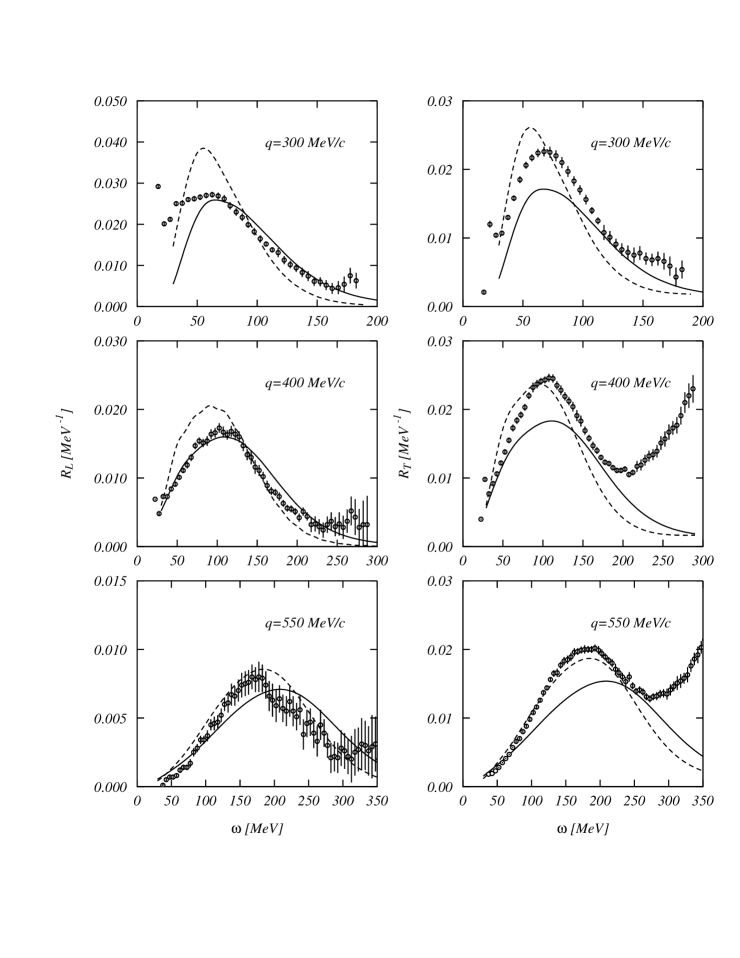
Figure 19: Comparison of the ¹²C experimental data of ref. [Bar83] with the CSM responses (dashed lines) and those obtained including the various corrections discussed in this paper, excluding the relativistic corrections.

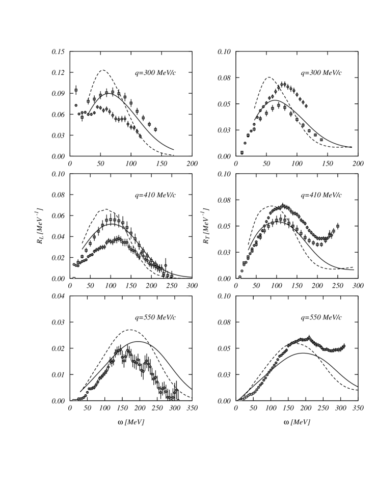
Figure 20: The same as the previous figure for ⁴⁰Ca. The data are from refs. [Mez84, Mez85] (circles) and [Yat93, Wil97] (squared).

In the standard treatment the longitudinal responses are overestimated while the transverse ones are reasonably well reproduced. This fact provoked disconcern since the electromagnetic operator generating the longitudinal response, the charge operator, is supposed to be better understood than the current operator.

A great theoretical effort has been done to explain the reduction of the longitudinal response. Various possibilities have been investigated, from relativistic effects [Cel85, Bro89a, Weh89, Hor90] to modifications of nucleon properties in the medium [Nob81, Nob83, Bro89b]. It is now generally accepted that the FSI is the mechanism responsible for the lowering of the longitudinal response. The same effect acts also on the transverse response destroying the previous agreement (as is shown by the full lines of the figs. 19 and 20. The problem now has been moved from the longitudinal to the transverse response whose empirical values are larger than those predicted.

A word of caution is necessary at this point. The responses are not directly measured but they are extracted from a set of cross section measurements. The extraction procedure is rather complicated and it is based upon various theoretical hypotheses on the structure and the behavior of the cross section. Some of the published data have been modified after a reanalysis [Jou95, Jou96]. The discussion on the reliability of the existing data and on the need of acquiring new ones is still open. It is not our intention to discuss this issue here.

We would like to remark however that the new set of ⁴⁰Ca data [Yat93, Wil97] (squares in fig. 20) agrees rather well with our calculations.

5 Conclusions

In this article we have discussed the validity of the approximations made in what we have called the standard description of the QE excitation. This is a PWBA calculation done within non relativistic MF nuclear model and using one-body currents only.

The PWBA is usually adopted because it leads to a simple expression of the cross section, which allows the separation of longitudinal and transverse responses through a Rosenbluth procedure. Distortion effects produced by the Coulomb field of the nucleus are not very big. For nuclei with $Z<20$ they can be rather well simulated by the effective momentum transfer prescription (26). For heavier nuclei the focusing of the electron wave function onto the nucleus becomes relevant and DWBA calculations are necessary [Co’87a, Tra88].

A major source of uncertainty in the electron-nucleus interaction is related to the choice of the electromagnetic nucleon form factors [Ama93a]. We have shown in fig. 3 the uncertainty band produced by the various possible choices.

The size of the two-body currents effects is within this uncertainty band. We have studied two-body currents produced by the exchange of one pion. We have seen that the total effect of these MEC on the response is small because of the cancelation between the seagull and pionic current contributions [Ama93b]. Seagull and pionic currents modify the response in opposite directions and the final effect is rather small. We have also evaluated the contribution of the currents associated to the excitation of a virtual $\Delta$ which has been found to lower the transverse response [Ama94a] but to be rather small.

An estimate of the effects produced by relativistic corrections shows that their size is within the form factor uncertainty band as long as the momentum transfer value remains smaller than 500 MeV/$c$ [Ama96a, Ama96b, Ama98a].

We started our investigation of the nuclear excitation mechanism by testing the need of using a finite system description for the QE excitation. We have compared CSM and FG responses and we found that they are rather similar if the value of the Fermi momentum is evaluated by considering the average nuclear density (see eq. (57)). The agreement worsen by using the LDA [Ama94b].

We have seen that RPA corrections are not important when a finite-range interaction is used [Co’88, Ama93b]. Zero-range interactions overestimate RPA effects, especially at high values of the momentum transfer. In infinite nuclear systems the choice of the residual interaction is inconsistent with the effective theory where it is used [Bau98a, Bau98b]. From a pragmatic point of view these uncertainties are irrelevant since RPA effects are small.

The largest correction to the standard description of the QE excitation is produced by the FSI. Microscopic calculations done within the second RPA framework indicates that, in the QE region, the FSI can be rather well described in terms of an imaginary part of the optical potential [Dro87]. We have developed an alternative approach to deal with FSI [Co’88]. Our results are similar to those obtained using the optical potential. The FSI enlarges the widths of the responses and lowers the peak values [Ama93b].

The comparison with the experimental ¹²C data [Bar83] shows that, when the FSI corrections are included, the longitudinal responses are reasonably well reproduced while the transverse one are underestimated [Ama94a]. The same kind of calculation in ⁴⁰Ca does not reproduce the Saclay data [Mez84, Mez85] while the new MIT data [Yat93, Wil97] are rather well described in both longitudinal and transverse responses.

There are various problems still unsolved in the study of the QE excitation. At present the longitudinal responses seem rather well understood but the transverse ones are underestimates. There are exclusive data [Ulm87, Ber90] indicating that the two-nucleon emission in the QE region could be larger than that predicted by the MEC [Ama93b]. This suggest the need of considering short-range correlations in the nuclear model [Fan87, Fab89, Lei90, Orl91, Fab94, Fab97, Ama98b, Co’98]. Also the so-called dip region, the region between the QE peak and the peak of the $\Delta$ resonance, is at present not well described.

The QE excitation of nuclei is a good testing ground of our knowledge of the electron-nucleus interaction and our understanding of the nuclear excitation mechanism. Since surface effects are not important [Ama94b] it is meaningful to compare directly the experimental data with the results of complicated many-body theories developed in infinite systems [Fan87, Alb89, Fab89, Cen94, Fab94, Cen97, Fab97].

We believe that the solution of the problems mentioned above and the interest of the theoreticians in comparing the results of their models with QE data require new accurate and reliable data which could be rather straightforwardly obtained at the new electron accelerator facilities.

References

- [Alb84] W. Alberico, M. Ericson and A. Molinari, Ann. Phys. (N.Y.) 154 (1984), 356.
- [Alb87a] W.M. Alberico, P. Czerski, M. Ericson and A. Molinari, Nucl. Phys. A 462 (1987), 269.
- [Alb87b] W.M. Alberico, G. Chanfray, M. Ericson and A. Molinari, Nucl. Phys. A 475 (1987), 233.
- [Alb89] W.M. Alberico, R. Cenni and A. Molinari, Prog. Part. Nucl. Phys. 23 (1989), 171.
- [Alb90] W.M. Alberico, T.W. Donnelly and A. Molinari, Nucl. Phys. A 512 (1990), 541.
- [Alt80] R. Altemus et al., Phys. Rev. Lett. 44 (1980), 965.
- [Ama92] J.E. Amaro, G. Co’, E.M.V. Fasanelli and A.M. Lallena, Phys. Lett. B 277 (1992), 249.
- [Ama93a] J.E. Amaro, “Efecto de los grados subnucleares de libertad en la respuesta cuasielástica nuclear”, Ph.D. Thesis , Universidad de Granada, 1993.
- [Ama93b] J.E. Amaro, G. Co’, and A.M. Lallena, Ann. Phys. (N.Y.) 221 (1993), 306.
- [Ama94a] J.E. Amaro, G. Co’, and A.M. Lallena, Nucl. Phys. A 578 (1994), 365.
- [Ama94b] J.E. Amaro, A.M. Lallena and G. Co’ Int. Jour. Mod. Phys. E 3 (1994), 735.
- [Ama96a] J.E. Amaro, J.A. Caballero, T.W. Donnelly, A.M. Lallena, E. Moya de Guerra and J.M. Udías, Nucl. Phys. A 602 (1996), 263.
- [Ama96b] J.E. Amaro, J.A. Caballero, T.W. Donnelly and E. Moya de Guerra, Nucl. Phys. A 611 (1996), 163.
- [Ama98a] J.E. Amaro and T.W. Donnelly, Ann. Phys. (NY) 263 (1998), 56.
- [Ama98b] J.E. Amaro, A.M. Lallena, G. Co’ and A. Fabrocini Phys. Rev. C 57 (1998) 3473.
- [Ama98c] J.E. Amaro, M.B. Barbaro, J.A. Caballero, T.W. Donnelly and A. Molinari, Nucl. Phys. A 643 (1998) 349
- [Bar83] P. Barreau et al., Nucl. Phys. A 402 (1983), 515; Note CEA-N-2334, Saclay (1983).
- [Bau98a] E. Bauer and A.M. Lallena, Phys. Rev. C 57 (1998) 1681.
- [Bau98b] E. Bauer and A.M. Lallena, submitted to Phys. Rev. C
- [Ber72] W. Bertozzi, J. Friar, J. Heisenberg and J.W. Negele, Phys. Lett. B 41 (1972), 408.
- [Ber87] A.M. Bernstein, Proceedings of the 3rd. Workshop on Perspectives in Nuclear Physics at Intermediate Energies (S. Boffi, C. Ciofi degli Atti and M. Giannini, Eds.), World Scientific, Singapore, 1987.
- [Ber90] W. Bertozzi , Proceedings of the Workshop on Two Nucleon Emission Reaction (O. Benhar and A. Fabrocini, Eds.), ETS Editrice, Pisa, 1990. , p.25
- [Bjo64] J.D. Bjorken and S.D. Drell, “Relativistic Quantum Mechanics”, McGraw-Hill, New York 1964.
- [Bla86] C. Blatchey et al., Phys. Rev. C 34 (1986), 1243.
- [Bof96] S. Boffi, C. Giusti, F.D. Pacati and M. Radici, Electromagnetic Response of Atomic Nuclei ,Clarendon Press, Oxford, 1996
- [Boh53] D. Bohm and D. Pines Phys. Rev92 (1953) 609.
- [Bou89] P.M. Boucher, B. Castel, Y. Okuhara and H. Sagawa, Ann. Phys. (N.Y.) 196 (1989), 150.
- [Bou91] P.M. Boucher and J.W. Van Orden, Phys. Rev. C 43 (1991), 582.
- [Bri87] F.A. Brieva and A. Dellafiore, Phys. Rev. C 36 (1987), 899.
- [Bro89a] R. Brokmann, D. Drechsel, J. Frank and P.G. Reinhard, Z. Phys. A 332 (1989), 51.
- [Bro89b] G.E. Brown and M. Rho, Phys. Lett. B 222 (1989), 324.
- [Bub91] M. Buballa, S. Drożdż, S. Krewald and J. Speth, Ann. Phys. (N.Y.) 208 (1991), 346.
- [Cap91] F. Capuzzi, C. Giusti and F.D. Pacati, Nucl. Phys. A 524 (1991), 681.
- [Cav84] M. Cavinato et al., Nucl. Phys. A 423 (1984), 376.
- [Cav90] M. Cavinato, M. Marangoni and A.M. Saruis, Phys. Lett. B 235 (1990), 346.
- [Cel85] L.S. Celenza, A. Harindranath and C.M. Shakin, Phys. Rev. C 32 (1985), 248.
- [Cen94] R. Cenni and P. Saracco, Phys. Rev. C 50 (1994) 1851.
- [Cen97] R. Cenni, F. Conte and P. Saracco, Nucl. Phys. A 623 (1997) 391.
- [Che71] M. Chemtob and M. Rho, Nucl. Phys. A 163 (1971), 1.
- [Chi89] C.R. Chinn, A. Picklesimer and J.W. Van Orden, Phys. Rev. C 40 (1989), 790; 1159.
- [Cio80] C. Ciofi degli Atti, Prog. Part. Nucl. Phys. 3 (1980), 163.
- [Co’84] G. Co’ and S. Krewald, Phys. Lett. B 137 (1984), 145.
- [Co’85] G. Co’ and S. Krewald, Nucl. Phys A 433 (1985), 392.
- [Co’87a] G. Co’ and J. Heisenberg, Phys. Lett. B 197 (1987), 489.
- [Co’87b] G. Co’, A.M. Lallena and T.W. Donnelly, Nucl. Phys. A 469 (1987), 684.
- [Co’88] G. Co’, K.Q. Quader, R. Smith and J. Wambach, Nucl. Phys. A 485 (1988), 61.
- [Co’98] G. Co’ and A.M. Lallena, Phys. Rev. C 57 (1998) 145.
- [Czy63] W. Czyż, Phys. Rev. 131 (1963), 2141.
- [Dea83] M. Deady et al., Phys. Rev. C 28 (1983), 631.
- [Dea86] M. Deady et al., Phys. Rev. C 33 (1986), 1897.
- [deF66] T. deForest and J.D. Walecka, Adv. Phys. 15 (1966), 57.
- [DeJ87] C.W. DeJager and C. DeVries, At. Data and Nucl. Data Tables 36 (1987), 495.
- [Del85] A. Dellafiore, F. Lenz and F.A. Brieva, Phys. Rev. C 31 (1985), 1088.
- [DeP93] A. DePace and M. Viviani, Phys. Rev. C 48 (1993) 2931.
- [Don75] T.W. Donnelly and J.D. Walecka, Ann. Rev. Nucl. Science 25 (1975), 329.
- [Dow88] K. Dow et al., Phys. Rev. Lett. 61 (1988), 1706.
- [Dre89] D. Drechsel and M.M. Giannini, Rep. Prog. Phys. 52 (1989) 1083.
- [Dro87] S. Drożdż, G. Co’, J. Wambach and J. Speth, Phys. Lett. B 185 (1987), 287.
- [Dro89] S. Drożdż, M. Buballa, S. Krewald and J. Speth, Nucl. Phys. A 501 (1989), 487.
- [Dro90] S. Drożdż, S. Nishizaki, J. Speth and J. Wambach Phys. Rep.197 (1990) 1.
- [Edm57] A.R. Edmonds,“Angular momentum in quantum mechanics”, Princeton University Press, Princeton, 1957.
- [Fan87] S. Fantoni and V.R. Pandharipande, Nucl. Phys. A 473 (1987), 234.
- [Fab89] A. Fabrocini and S. Fantoni, Nucl. Phys. A 503 (1989), 375.
- [Fab94] A. Fabrocini, Phys. Lett. B 322 (1994) 171.
- [Fab97] A. Fabrocini, Phys. Rev. C 55 (1997) 338.
- [Fri77] J.L.Friar, Phys. Lett. B 69 (1977), 51.
- [Gar76] M. Gari and H. Hyuga, Z. Phys. A 277 (1976), 291; Nucl. Phys. A 274 (1976), 333.
- [Gar92] C. Garcia-Recio, J. Navarro, N. Van Giai and L.L. Salcedo, Ann. Phys. (NY) 214 (1992) 293.
- [Gil97] A. Gil, J. Nieves and E. Oset, Nucl. Phys. A 627 (1997) 543.
- [Hei83] J. Heisenberg and H.P. Blok, Ann. Rev. Nucl. Part. Sc. 33 (1983), 569
- [Hoc73] J. Hockert, D.O. Riska, M. Gari and A. Huffman, Nucl.Phys. A 217 (1973), 14.
- [Hoe76] G. Hoehler et al., Nucl. Phys. B 114 (1976), 505.
- [Hor80] Y. Horikawa, F. Lenz and N.C. Mukhopadhyay, Phys. Rev. C22 (1980) 461.
- [Hor90] C.J. Horowitz and J. Piekarewicz, Nucl. Phys. A 511 (1990), 461.
- [Hot84] A. Hotta et al., Phys. Rev. C 30 (1984), 87.
- [Iac73] F. Iachello, A.D. Jackson and A. Lande, Phys. Lett. B 43 (1973), 191.
- [Jan66] T. Janssens, R. Hofstadter, E.B. Hughes and M.R. Yearian, Phys. Rev. 142 (1966), 922.
- [Jes94] S. Jeschonnek, A. Szczurek, G. Co’ and S. Krewald, Nucl. Phys. A 570 (1994) 599.
- [Jes98] S. Jeschonnek and T. W. Donnelly, Phys. Rev. CC57 (1998) 2438.
- [Jou95] J. Jourdan, Phys. Lett. B 353 (1995) 189.
- [Jou96] J. Jourdan, Nucl. Phys. A 603 (1996) 117.
- [Koh81] M. Kohno and N. Ohtsuka, Phys. Lett. B 98 (1981), 335.
- [Koh83] M. Kohno, Nucl. Phys. A 410 (1983), 349.
- [Lal97] A.M. Lallena, Nucl. Phys. A 615, (1997) 325.
- [Lei90] W. Leidemann and G. Orlandini, Nucl. Phys. A506 (1990) 447.
- [Loc75] J.A. Lock and L.L. Foldy, Ann. Phys. 93 (1975), 276.
- [Mah82] C. Mahaux and N. Ngô, Nucl. Phys. A 378 (1982), 205. Note CEA-N-2439, Saclay (1985).
- [Mez84] Z.E. Meziani et al., Phys. Rev. Lett. 52 (1984), 2130.
- [Mez85] Z.E. Meziani et al., Phys. Rev. Lett. 54 (1985), 1233; DPhN n0 2292, Saclay (1984).
- [Mig57] A.B. Migdal,Theory of Finite Fermi Systems and Applications to Atomic Nuclei, Interscience, New York, 1957.
- [Mon69] E.J. Moniz, Phys. Rev. 184 (1969), 1154.
- [Mon71] E.J. Moniz et al., Phys. Rev. Lett. 26 (1971), 445.
- [Nob81] J.V. Noble, Phys. Rev. Lett. 46 (1981), 412.
- [Nob83] J.V. Noble, Phys. Rev. C 27 (1983), 423.
- [Orl91] G. Orlandini and M. Traini, Rep. Prog. Phys. 54 (1991), 257.
- [Pec69] R.D. Peccei, Phys. Rev. 181 (1969), 1902.
- [Pin88a] D. Pines, K.Q. Quader and J. Wambach, Nucl. Phys. A 469 (1988), 365
- [Pin88b] D. Pines, K.Q. Quader and J. Wambach, Nucl. Phys. A 477 (1988), 365.
- [Ris79] D.O. Riska, en “Mesons in nuclei, Vol.II” (M. Rho and D. Wilkinson, Eds.), North-Holland, Amsterdam, 1979.
- [Ris84] D.O. Riska, Prog. Part. Nucl. Phys., 11 (1984), 199.
- [Ros50] M.N. Rosenbluth, Phys. Rev. 79 (1950), 615.
- [Sag89] H. Sagawa, P.M. Boucher, B. Castel and Y. Okuhara, Phys. Lett. B 219 (1989), 10.
- [Sar93] A.M. Saruis, Phys. Rep. 235 (1993) 57.
- [Sch89] R. Schiavilla, V.R. Pandharipande and D.O. Riska, Phys. Rev. C 40 (1989), 2224.
- [Shi89] T. Shigehara, K. Shimizu and A. Arima, Nucl. Phys. A 492 (1989), 388.
- [Sim80] G.G. Simon, Ch. Schmitt, F. Borkowski and V.H. Walther, Nucl. Phys. A 333 (1980), 381.
- [Sky56] T.H.R. Skyrme, Phil. Mag.1 (1956) 1043.
- [Tra88] M. Traini, S. Turck-Chièze and A. Zghiche Phys. Rev. C38 (1988), 2799.
- [Tra93] M. Traini, G. Orlandini and W. Leidemann, Phys. Rev. C 48 (1993) 172.
- [Ulm87] P.E. Ulmer et al, Phys. Rev. Lett. 59 (1987) 2259.
- [Vau72] D. Vautherin and D. Brink, Phys. Rev. C 5 (1972) 626.
- [Van81] J.W. Van Orden and T.W. Donnelly, Ann. Phys. (N.Y.) 131 (1981), 451.
- [Van95] V. Van der Sluys, J. Ryckebush and M. Waroquier, Phys. Rev. C 51 (1995) 2664.
- [Voy62] K.W. McVoy and L. Van Hove, Phys. Rev. 125 (1962) 1034.
- [War87] M. Waroquier et al., Phys. Rep. 148 (1987) 249.
- [Weh89] K. Wehrberger and F. Beck, Nucl. Phys. A 491 (1989), 587.
- [Wil97] C.F.Wiliamson et al., Phys. Rev. C 56 (1997) 3152.
- [Yat93] T.C.Yates et al., Phys. Lett. B 312 (1993), 382.
- [Yan82] C. Yannouleas, M. Dworrzecka and J.J. Griffin, Nucl. Phys. A 379 (1982) 256.
- [Yan83] C. Yannouleas, M. Dworrzecka and J.J. Griffin, Nucl. Phys. A 397 (1983) 239.
- [Yen54] D.R. Yennie, D.G. Ravenhall and R.N. Wilson, Phys. Rev. 95 (1954), 500.
- [Zgh94] A. Zghiche et al., Nucl. Phys. A 572 (1994) 513.