Proton-Proton Fusion in Leading Order of

Effective Field Theory

Xinwei Kong¹ and Finn Ravndal

Department of Physics and Institute of Nuclear Theory,

University of Washington, Seattle, WA 98195, U.S.A

Abstract: Using a recently developed effective field theory for the interactions of nucleons at non-relativistic energies, we calculate the rate for the fusion process $p+p\rightarrow d+e^{+}+\nu_{e}$ to leading order in the momentum expansion. Coulomb effects are included non-perturbatively in a systematic way. The resulting rate is independent of specific models for the strong interactions at short distances and is in agreement with the standard result in the zero-range approximation.

The first step in the different nuclear processes in the Sun which generate the observed luminosity is proton-proton fusion $p+p\rightarrow d+e^{+}+\nu_{e}$[1]. It was explained more than sixty years ago by Bethe and Critchfield[2] when nuclear physics was still in its infancy. When the field had more matured, it was reconsidered in the light of more modern developments by Salpeter[3] and later by Bahcall and May[4]. But in spite of the enormous progress in nuclear physics during this time, the methods and approximations made in these different calculations were essentially the same. The obtained accuracy in the obtained fusion rate was just a few percent. Including higher order electromagnetic and strong corrections the uncertainty in the rate is now around one percent[5][6]. This is very impressive for a strongly interacting process at low energies very ordinary perturbation theory cannot be used.

In the light of the importance this fundamental process plays in connection with the solar neutrino problem and possible neutrino oscillations[1], it is natural to reconsider this process from the point of view of modern quantum field theory instead of the old potential models used previously. A first attempt in this direction was made by Ivanov et al.[7]. They obtained then a result which was significantly different from the standard result based upon potential models. Subsequently it was pointed out by Bahcall and Kamionowski[8] that their effective nuclear interaction was not consistent with what is known about proton-proton scattering at low energies where Coulomb effects are important.

The approach of Ivanov et al.[7] is based upon relativistic field theory and should in principle yield reliable results. But it is well known that in particular for bound states like the deuteron it is very difficult to use consistently a relativistic formulation. Also the uncertain nuclear physics part of the fusion process under consideration takes place at low energies and should therefore be described within a non-relativistic framework. Then all the large-momentum degrees of freedom are integrated out and one is left with an effective theory involving only the physically important field variables. The underlying, relativistic interactions are then replaced by non-renormalizable local interactions with coupling constants which must be determined from experiments at low energies. In such a non-relativistic theory the important Coulomb effects can also systematically be included.

A step in this direction has recently been taken by Park et al. using chiral perturbation theory in the low-energy limit[9]. They obtain results in very good agreement with previous potential calculations which is not so surprising since they make use of phenomenological nucleon wavefunctions which fit low-energy scattering data very well. A more fundamental approach to the same problem has recently been formulated by Kaplan, Savage and Wise in terms of an effective theory for non-relativistic nucleons[10]. It involves a few basic coupling constants which have been determined from nucleon scattering data at low energies. With no more free parameters it can then be used to make predictions for the deuteron form factor and quadrupole moment[11], deuteron polarizabilities and Compton scattering on deuterons[12]. The obtained results are in good agreement with experimental data. In this approach higher order corrections can also be derived in a systematic way. Going to higher energies, the effects of pions must be included using the established counting rules. These will cause the well-known $D$-mixture into the deuteron wavefunction.

Most recently, proton-neutron fusion $p+n\rightarrow d+\gamma$ has been calculated in this theory by Savage, Scaldeferri and Wise[13] including the effects of virtual pions. When the process is taking place at very low energies, one can omit the effects of pions and replace them by slightly different couplings of the nucleons alone. From a field-theoretic point of view this process is very similar to $p+p\rightarrow d+e^{+}+\nu_{e}$. The main difference is the strong Coulomb effects which is present in the proton-proton channel. These have now been calculated and shown to give both a scattering length and an effective range for $pp$ low-energy scattering in agreement with data[15]. Based upon these results, we will here derive the rate for the corresponding $pp$ fusion reaction. This same process is also being considered by Savage and Wise[14]. At this stage we are only interested in the dominant contributions to the fusion rate in order to provide a rough comparison with results based upon potential models. This corresponds to the zero-range approximation in the potential model approach. In light of previous applications, we expect the resulting accuracy to be around 20% or better in the resulting rate. In this leading order approximation we ignore effective-range corrections, $D$-wave admixture, vacuum polarization, two-body current interactions and unknown counterterms.

The strong interactions among the nucleons are now described by the effective Lagrangian of Kaplan, Savage and Wise[10]. Denoting the nucleon field of mass $M$ by $N(x)$ and including only the lowest order interaction term in the $S$-channel, it can be written as

$${\cal L}=N^{\dagger}\left(\partial_{t}+{\nabla^{2}\over 2M}\right)N-C_{0}(N^{T}{\mbox{\boldmath$\Pi$}}N)\cdot(N^{T}{\mbox{\boldmath$\Pi$}}N)^{\dagger}$$ (1)

where the $\Pi_{i}$ are projection operators into specific spin and isospin states. More specifically, for spin-singlet interactions $\Pi_{i}=\sigma_{2}\tau_{2}\tau_{i}/\sqrt{8}$ while for spin-triplet interactions $\Pi_{i}=\sigma_{2}\sigma_{i}\tau_{2}/\sqrt{8}$. Calculating now the scattering amplitude for two nucleons, one finds that the coupling constant $C_{0}$ is determined by the scattering length $a_{NN}$ in this channel[10].

For neutron-proton interactions in the spin-triplet channel there is pole in the corresponding Green’s function corresponding to the deuteron. The residue of the pole gives the bound state wavefunction. With only the lowest order contact interaction in (1) it is found to be of the form

$$\psi_{d}({\bf k})={\sqrt{8\pi\gamma}\over{\bf k}^{2}+\gamma^{2}}$$ (2)

in momentum space. This corresponds to the standard Yukawa form in coordinate space where $1/\gamma$ represents the size of the deuteron. It determines the value of the corresponding coupling constant $C_{0}$ in this channel[11].

In the absence of strong interactions, the incoming proton-proton state with center-of-mass momentum ${\bf p}$ is given by the Coulomb wavefunction[16]

$$\psi_{\bf p}({\bf r})={1\over\rho}\sum_{\ell=0}^{\infty}(2\ell+1)i^{\ell}e^{i\sigma_{\ell}}F_{\ell}(\rho)P_{\ell}(\cos(\theta)$$ (3)

Here $\rho=pr$ and $\sigma_{\ell}=\arg{\Gamma(1+\ell+i\eta)}$ is the Coulomb phaseshift where the parameter $\eta=\alpha M/2p$ characterizes the strength of the Coulomb interaction. At low energies only the $S$-wave will contribute. It is given in terms of the confluent hypergeometric or Kummer function $M(a,b;z)$ as

$$F_{0}(\rho)=C_{\eta}\rho e^{-i\rho}M(1-i\eta,2;2i\rho)$$ (4)

where the normalization factor $C_{\eta}=e^{-\pi\eta/2}|\Gamma(1+i\eta)|$. The probability $|\psi_{\bf p}(0)|^{2}$ to find the two protons at the same point is thus equal to the Sommerfeld factor[17]

$$C_{\eta}^{2}={2\pi\eta\over e^{2\pi\eta}-1}$$ (5)

At very low energies when $\eta$ gets large it becomes exponentially small and is the dominant effect in the fusion reaction.

The available energy in the process is set by the neutron-proton mass difference and the deuteron binding energy $B$ = 2.225 MeV. It corresponds to a momentum $\gamma=\sqrt{BM}$ of the bound nucleons equal to 45.71 MeV. The temperature in the core of the Sun is approximately $15\times 10^{6}$ K which corresponds to an average proton momentum around $p=1.5$  MeV. The kinetic energy of the lepton pair will therefore be much smaller than $\gamma$ and it is a very good approximation to just ignore it. In the following the weak current is therefore assumed to carry zero momentum and the evaluation of the different Feynman diagrams will much simplify.

To lowest order in the strong interaction between the protons, the transition matrix $T_{fi}$ is given by the first diagram in Fig.1. After being hit by the weak current, the proton-proton system is transformed into a bound deuteron. The value of the diagram is thus seen to be

$$A(p)=\sqrt{8\pi\gamma}\int\!{d^{3}k\over(2\pi)^{3}}{1\over{\bf k}^{2}+\gamma^{2}}\psi_{\bf p}({\bf k})$$ (6)

where $\psi_{\bf p}({\bf k})$ is the Fourier transformed wavefunction of the incoming proton-proton scattering state. To first order in the four-proton ${}^{1}S_{1}$ coupling $C_{0}$ we have the diagram in Fig. 1b.

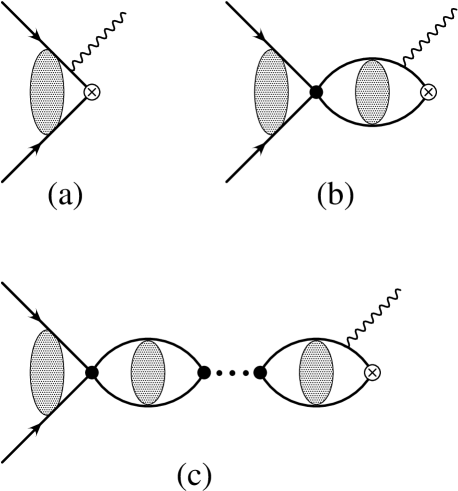
Figure 1: Feynman diagrams which contribute in leading order to proton-proton fusion. The solid lines are nucleons and the wiggly line represents the weak current. Between the protons there are exchanged Coulomb photons represented by the shaded blobs while the crossed circles represents the deuteron wavefunctions.

Within the loop the protons move in the Coulomb field of each other. This motion is described by the standard Coulomb propagator $G_{C}(E)=1/(E-H_{0}-V_{C}+i\epsilon)$ where $H_{0}$ is the free, non-relativistic Hamiltonian and $V_{C}$ is the Coulomb potential. In momentum space it takes the form

$$G_{C}(E;{\bf k},{\bf k}^{\prime})=M\!\int\!{d^{3}q\over(2\pi)^{3}}{\psi_{\bf q}({\bf k})\psi_{\bf q}^{*}({\bf k}^{\prime})\over{\bf p}^{2}-{\bf q}^{2}+i\epsilon}$$ (7)

when expressed in terms of the Coulomb wavefunctions for the center-of-mass energy $E=p^{2}/M$. As illustrated in Fig.2 it includes the free propagator plus the effects

Figure 2: The full Coulomb propagator is formed from the infinite sum of exchanged static photons.

of one, two and more exchanged static photons. In this way we find for the diagram in Fig.1b the value $C_{0}B(p)$ where

$$B(p)=\sqrt{8\pi\gamma}\int\!{d^{3}k\over(2\pi)^{3}}{d^{3}k^{\prime}\over(2\pi)^{3}}{1\over{\bf k}^{2}+\gamma^{2}}G_{C}(E;{\bf k},{\bf k}^{\prime})$$ (8)

is a convergent integral.

The protons can suffer another rescattering as in Fig.1c before they are converted to a deuteron by the weak interaction. Denoting this extra bubble in the diagram by $J_{0}(p)$, the full diagram is then just $C_{0}J_{0}$ times the previous diagram. The magnitude of the bubble equals the probability amplitude for the two protons to propagate from zero spatial separation back to zero separation, i.e. $J_{0}(p)=G_{C}(E;0,0)$. In terms of the representation (7) of the Coulomb propagator it is given by the integral

$$J_{0}(p)=M\!\int\!{d^{3}q\over(2\pi)^{3}}{2\pi\eta(q)\over e^{2\pi\eta(q)}-1}{1\over p^{2}-q^{2}+i\epsilon}$$ (9)

which has an ultraviolet divergence. After regularization, it will give a renormalization of the coupling constant $C_{0}$.

We can now continue to add in more such rescattering diagrams in Fig.1c. They form a geometric series which sums up to $C_{0}/(1-C_{0}J_{0})$. All the diagrams including the first then gives for the hadronic part of the full transition amplitude

$$T_{fi}(p)=A(p)+B(p){C_{0}\over 1-C_{0}J_{0}(p)}\psi_{\bf p}(0)$$ (10)

where the last factor $\psi_{\bf p}(0)=C_{\eta}e^{i\sigma_{0}}$ gives the amplitude for the two incoming protons to meet at the first vertex. It can be written in a more compact and recognizable form by introducing the proton-proton scattering state

$$\mbox{$\mid\!\Psi_{\bf p}\rangle$}=[1+\sum_{n=1}^{\infty}(G_{C}V_{0})^{n}]\mbox{$\mid\!\psi_{\bf p}\rangle$}$$ (11)

where the strong interaction potential $\mbox{$\langle{\bf p}\!\mid$}V_{0}\mbox{$\mid\!{\bf q}\rangle$}=C_{0}$ is included to all orders in addition to the Coulomb interaction. Then we see that the matrix element (10) is just the overlap integral between this wavefunction and the deuteron wavefunction (2),

$$T_{fi}(p)=\int\!{d^{3}k\over(2\pi)^{3}}\psi_{d}^{*}({\bf k})\Psi_{\bf p}({\bf k})$$ (12)

as follows from the expressions in (6) and (8). This form of the transition matrix element was written down first by Bethe and Chritchfield[2] and used subsequently by everyone considering the process in potential models.

We can now evaluate the different parts of the transition matrix element (10). The first part (6) is most easily found in coordinate space where we have the Coulomb wavefunction (4). It gives

$$A(p) = \sqrt{8\pi\gamma}C_{\eta}e^{i\sigma_{0}}\int_{0}^{\infty}\!drre^{-(\gamma+ip)r}M(1-i\eta,2;2ipr)$$

$$= {\sqrt{8\pi\gamma}C_{\eta}e^{i\sigma_{0}}\over(\gamma+ip)^{2}}{{}_{2}F_{1}}\left(1-i\eta,2;2;{2ip\over\gamma+ip}\right)$$

Now the hypergeometric function ${}_{2}F_{1}(a,b,b;z)=(1-z)^{-a}$ so that the final result can be written as

$$A(p)=C_{\eta}e^{i\sigma_{0}}{\sqrt{8\pi\gamma}\over p^{2}+\gamma^{2}}e^{2\eta\arctan({p\over\gamma})}$$ (14)

In the expression (8) for $B(p)$ we notice that the integral over ${\bf k}^{\prime}$ gives the complex conjugate value of the Coulomb wavefunction at the origin. It therefore takes the form

$$B(p)=M\int\!{d^{3}k\over(2\pi)^{3}}\int\!{d^{3}q\over(2\pi)^{3}}{\sqrt{8\pi\gamma}\over{\bf k}^{2}+\gamma^{2}}{\psi_{\bf q}({\bf k})\over{\bf p}^{2}-{\bf q}^{2}+i\epsilon}\psi_{\bf q}^{*}(0)$$

The integral over ${\bf k}$ is just the previous result for $A(q)$ so that

$$B(p)=M\int\!{d^{3}q\over(2\pi)^{3}}{\sqrt{8\pi\gamma}\over q^{2}+\gamma^{2}}{e^{2\eta\arctan({q\over\gamma})}\over p^{2}-q^{2}+i\epsilon}{2\pi\eta(q)\over e^{2\pi\eta(q)}-1}$$ (15)

It is seen that when the momentum of the incoming protons is non-zero the integral yields a complex result.

The infinite sum over proton bubble diagrams in Fig.1 is just the proton-proton strong scattering amplitude modified by Coulomb corrections[15]. It is given by the bubble integral (9). In order to regularize it we use the special PDS scheme constructed by Kaplan, Savage and Wise for this effective theory[10]. It is based on ordinary dimensional regularization around $d=3$ dimensions. The difference lies in that poles in $d=2$ dimensions are subtracted. This gives rise to terms which depend on the regularization point $\mu$. In the present case we obtain with $\epsilon=3-d$

$$J_{0}(p)={\alpha M^{2}\over 4\pi}\left[{1\over\epsilon}+\ln{\mu\sqrt{\pi}\over\alpha M}+1-{3\over 2}C_{E}-H(\eta)\right]-{\mu M\over 4\pi}$$ (16)

Here $C_{E}=0.5772\ldots$ is Euler’s constant and the function

$$H(\eta)=\psi(i\eta)+{1\over 2i\eta}-\ln(i\eta)$$ (17)

The divergent $1/\epsilon$ piece will be absorbed in counterterms representing electromagnetic interactions at shorter scales. This replaces the bare coupling constant $C_{0}$ with the renormalized value $C_{0}(\mu)$. Matching the calculated proton-proton scattering amplitude to the experimental one, we can determine this coupling constant in terms of the measured scattering length $a_{p}$ which gives the cross-section in the zero-energy limit[15],

$${4\pi\over MC_{0}(\mu)}={1\over a_{p}}-\mu+\alpha M\left[\ln{\mu\sqrt{\pi}\over\alpha M}+1-{3\over 2}C_{E}\right]$$ (18)

The part of the scattering amplitude which is needed in (10) is therefore

$$C_{0}^{-1}(\mu)-J_{0}(p)={M\over 4\pi}\left[{1\over a_{p}}+\alpha MH(\eta)\right]$$ (19)

This is in general complex because of the function (17). Its real part is the more phenomenologically relevant function $h(\eta)=\mbox{Re}\,\psi(i\eta)-\ln\eta$ while the imaginary part is simply $C_{\eta}^{2}/2\eta$. At very low energies the real part $h(\eta)=1/(12\eta^{2})+{\cal O}(\eta^{-4})$ dominates since the imaginary part is then exponentially small. These functions are well-known in the context of proton-proton scattering[18].

For the very small proton momenta we have in the Sun, one evaluates the transition matrix element just as well at zero momentum[4]. The first term (14) is then simply

$$|A(p\rightarrow 0)|=\sqrt{\frac{8\pi C_{\eta}^{2}}{\gamma^{3}}}\,e^{\chi}$$ (20)

where the parameter $\chi=\alpha M/\gamma$. It is therefore natural to introduce the standard reduced matrix element[3]

$$\Lambda(p)=\sqrt{{\gamma^{3}\over 8\pi C_{\eta}^{2}}}\,|T_{fi}(p)|$$ (21)

Using $2\pi\eta(q)$ as a new integration variable in the expression (15) for $B(p\rightarrow 0)$, it becomes proportional to the integral

$$I(\chi)=\int_{0}^{\infty}\!dx{2x\over e^{x}-1}{e^{{x\over\pi}\arctan({\pi\chi\over x})}\over x^{2}+\pi^{2}\chi^{2}}$$ (22)

which we can only do numerically. We thus have the result

$$\Lambda(0)=e^{\chi}-\alpha Ma_{p}\,I(\chi)$$ (23)

The first part is identical with what one obtains in potential models[4] while the second part seems to have a different dependence on the parameter $\chi$. However, by numerical integration, we find that it is in fact exactly the same. So far we have been unable to show this equality by analytical methods.

However, it can be demonstrated by taking first the zero energy limit of the proton-proton wavefunction in the integrand of the transition matrix element (12) and then afterwards integrate. The regular Coulomb wavefunction (4) simplifies then to[16]

$$F_{0}(\rho)\simeq{C_{\eta}\over\sqrt{2\eta}}\rho^{1/2}I_{1}(2\sqrt{2\eta\rho})$$ (24)

when $2\eta\gg\rho$. The first part (6) of the matrix element will now be given by the integral

$$A(p\rightarrow 0)=C_{\eta}e^{i\sigma_{0}}\sqrt{\frac{4\pi\gamma}{\eta}}{1\over p^{2}}\int_{0}^{\infty}\!d\rho\rho^{1/2}e^{-\gamma\rho/p}I_{1}(2\sqrt{2\eta\rho})$$

which can be expressed in terms of a Whittaker function,

$$|A(p\rightarrow 0)|=\sqrt{\frac{8\pi C_{\eta}^{2}}{\gamma^{3}}}\frac{e^{\chi/2}}{\chi}M_{-1,{1\over 2}}(\chi)$$

Now $M_{-1,{1\over 2}}(\chi)=\chi e^{\chi/2}$ and thus we reproduce the first part of (23).

In order to calculate $B(p\rightarrow 0)$ we go back to the result (8). Now we use a different representation of the Coulomb propagator constructed from the regular $F_{\ell}(\rho)$ and the irregular $G_{\ell}(\rho)$ eigenfunctions[19]. We only need the radial part in the $S$-channel

$$G_{C}(E;r,r^{\prime})_{\ell=0}=-{Mp\over 4\pi}{F_{0}(\rho_{<})\over\rho_{<}}{G_{0}(\rho_{>})\over\rho_{>}}$$ (25)

where $r_{<}$ and $r_{>}$ are the smallest and largest of $r$ and $r^{\prime}$ respectively. The irregular solution $G_{\ell}(\rho)$ is normalized so that the Wronskian $G_{0}F_{0}^{{}^{\prime}}-F_{0}G_{0}^{{}^{\prime}}=1$. In (8) this Green’s function is seen to enter with the argument $r^{\prime}=0$. Since $F_{0}(\rho)/\rho=C_{\eta}$ in the limit $\rho\rightarrow 0$, it then simplifies to

$$G_{C}(E;r,0)_{\ell=0}=-C_{\eta}{MpG_{0}(\rho)\over 4\pi\rho}$$

In the zero-energy limit $2\eta\gg\rho$ we can then use

$$G_{0}(\rho)\simeq{2\over C_{\eta}}\sqrt{2\eta\rho}K_{1}(2\sqrt{2\eta\rho})$$ (26)

For the function $B(p)$ we thus find in this limit

$$B(p\rightarrow 0)=-{M\over p}\sqrt{4\gamma\eta\over\pi}\int_{0}^{\infty}\!d\rho\rho^{1/2}e^{-\gamma\rho/p}K_{1}(2\sqrt{2\eta\rho})$$

This integral is now given by the other Whittaker function,

$$B(p\rightarrow 0)=-\frac{M^{2}\alpha}{4\pi}\sqrt{\frac{8\pi}{\gamma^{3}}}\frac{e^{\chi/2}}{\chi}W_{-1,{1\over 2}}(\chi)$$

Since $W_{-1,{1\over 2}}(\chi)=W_{-1,-{1\over 2}}(\chi)$ we can thus express the result by the simpler integral

$$W_{-1,-{1\over 2}}(\chi)=\chi e^{\chi/2}\int_{\chi}^{\infty}\!dt{e^{-t}\over t^{2}}$$ (27)

By partial integration it can be written in terms of the exponential integral function $E_{1}(\chi)$. In this way we finally obtain for the original integral (22)

$$I(\chi)={1\over\chi}-e^{\chi}E_{1}(\chi)$$ (28)

in agreement with the standard result[4].

With the previous value $\gamma=45.71\,$MeV for the deuteron, we have $\chi=0.15$ and the integral $I(0.15)=4.96$. Combined with the measured value $a_{p}=-7.82$ fm for the scattering length we then have $\Lambda(0)=2.51$ for the reduced matrix element. A recent and most accurate calculation including higher order corrections based on a potential model[6] gives a value $\Lambda^{2}(0)=7.05\pm 0.02$. This corresponds to $\Lambda(0)=2.66$. Our leading order result from effective field theory which we have found to agree with the zero-range approximation of potential models, is thus accurate to within 6% percent of the full result.

In next order of the momentum expansion of the underlying effective field theory it is not clear if the transition matrix element can still be given as a simple overlap integral of the two wavefunctions as in (12). The corresponding Feynman diagrams for the transition matrix element are also technically more difficult to evaluate because they involve the Coulomb propagator in new ways. But it is important to calculate these corrections and verify that they are as small as is found in potential models.

We want to thank John Bahcall, Jiunn-Wei Chen, Harald Griesshammer, Daniel Phillips, Martin Savage and Mark Wise for many helpful discussions and comments. In addition, we want to thank the Department of Physics and the INT for generous support and hospitality. Xinwei Kong is supported by the Research Council of Norway.

References

- [1] J.N. Bahcall, Neutrino Astrophysics, Cambridge University Press, Cambridge, 1989.
- [2] H.A. Bethe and C.L. Chritchfield, Phys. Rev. 54, 248 (1938).
- [3] E.E. Salpeter, Phys. Rev. 88, 547 (1952).
- [4] J.N. Bahcall and R.M. May, Ap. J. 155, 501 (1969).
- [5] M. Kamionkowski and J.N. Bahcall Ap. J. 420, 884 (1994).
- [6] R. Schiavilla, V.G.J. Stoks, W. Glöckle, H. Kamada, A. Nogga, J. Carlson, R. Machleidt, V.R. Pandharipande, R.B. Wiringa, A. Kievsky, S. Rosati and M. Viviani, Phys. Rev. C58, 1263 (1998).
- [7] A.N. Ivanov, N.I. Troitskaya, M. Faber and H. Oberhummer, Nucl. Phys. A617, 414 (1997); Errata ibid. A618, 509 and A625 896; H. Oberhummer, A.N. Ivanov, N.I. Troitskaya and M. Faber, astro-ph/9705119.
- [8] J.N. Bahcall and M. Kamionkowski, Nucl. Phys. A625, 893 (1997).
- [9] T.-S. Park, K. Kubodera, D.-P. Min and M. Rho, astro-ph/9804144.
- [10] D.B. Kaplan, M.J. Savage and M.B. Wise, Phys. Lett. B424, 390 (1998); Nucl. Phys. B534, 329 (1998).
- [11] D.B. Kaplan, M.J. Savage and M.B. Wise, Phys. Rev. C59, 617 (1999).
- [12] J.-W. Chen, H.W. Griesshammer, M.J. Savage and R.P. Springer, Nucl. Phys. A644, 221 (1998); ibid. A644, 245 (1998).
- [13] M.J. Savage, K.A. Scaldeferri and M.B. Wise, nucl-th/9811029.
- [14] M.J. Savage and M.B. Wise, unpublished.
- [15] X. Kong and F. Ravndal, nucl-th/9811076, to be published in Phys. Lett. B.
- [16] M. Abramowitz and I.A. Stegun, Handbook of Mathematical Functions, Dover Publications, Inc., New York, 1972.
- [17] A. Sommerfeld, Atombau und Spektrallinien, Vol. II, Vieweg, Braunschweig, 1939; L.D. Landau and E.M. Lifschitz, Quantum Mechanics, Pergamon Press, London, 1958.
- [18] J.D. Jackson and J.M. Blatt, Rev. Mod. Phys. 22, 77 (1950).
- [19] L.S. Brown and R.F. Sawyer, Ap. J. 489, 968 (1987); J.D. Jackson, Classical Electrodynamics, John Wiley & Sons, New York, 1975.