Particle Interferometry
for Relativistic Heavy-Ion Collisionsthanks: Columbia University preprint CU-TP-931, CERN report CERN-TH/99-15;   submitted to Physics Reports

Urs Achim Wiedemanna and Ulrich Heinzb,c

aPhysics Department, Columbia University,
New York, NY 10027, USA
bTheory Division, CERN, CH-1211 Geneva 23, Switzerland
cInstitut für Theoretische Physik, Universität Regensburg,
D-93040 Regensburg, Germany
Abstract

In this report we give a detailed account on Hanbury Brown/Twiss (HBT) particle interferometric methods for relativistic heavy-ion collisions. These exploit identical two-particle correlations to gain access to the space-time geometry and dynamics of the final freeze-out stage. The connection between the measured correlations in momentum space and the phase-space structure of the particle emitter is established, both with and without final state interactions. Suitable Gaussian parametrizations for the two-particle correlation function are derived and the physical interpretation of their parameters is explained. After reviewing various model studies, we show how a combined analysis of single- and two-particle spectra allows to reconstruct the final state of relativistic heavy-ion collisions.

Chapter 1 Introduction

By now, a large collection of experimental data exists from the first relativistic collisions between truly heavy ions [135], using the 11 GeV/nucleon gold beams from the Brookhaven AGS and the 160 GeV/nucleon lead beams from the CERN SPS. The first relativistic heavy-ion collider RHIC at BNL will soon start taking data at $\sqrt{s}=200$ $A$ GeV, and in the next decade, the already approved LHC program at CERN will explore relativistic heavy-ion collisions at even higher energies ($\sqrt{s}=5.5\,A$ TeV). The aim of this large scale experimental effort is to investigate the equilibration processes of hadronic matter and to test in this way the hadronic partition function at extreme energy densities and temperatures. Especially, one expects under sufficiently extreme conditions the transition to a new state of hadronic matter, the quark gluon plasma (QGP) in which the physical degrees of freedom of equilibration processes are partonic rather than hadronic [151, 66, 139, 109]. QCD lattice simulations predict this transition to occur at a temperature of approximately 150 MeV [97]. The experimental confirmation of a possibly created QGP is, however, difficult, since only very few particle species, mainly leptons, can provide direct information about the initial partonic stage of the collision. The much more abundant hadrons are substantially affected by secondary interactions and decouple from the collision region only during the final ‘freeze-out’ stage. A successful dynamical model of relativistic heavy-ion collisions should finally explain all these different observables, their dependence on the incident energy, impact parameter, and atomic number of the projectile and target nuclei.

At the present stage, theoretical efforts concentrate on discriminating between different models by comparing them with characteristic observables [135, 136, 76, 19]. The observed enhancement of strange hadron and low-mass dilepton yields and the measured $J/\Psi$-suppression provide strong indications that a dense system was created in the collision whose extreme condition has significantly affected particle production mechanisms. Furthermore, various observations signal collective (hydro)dynamical behaviour in the collision region which in turn indicates the importance of equilibration processes for the understanding of the collision dynamics. Especially, the hadronic momentum spectra show signs of both radial and azimuthally directed flow, and two-particle correlations indicate a strong transverse expansion of the source before freeze-out. Despite the rich body of these and other observations, it remains however controversial to what extent these data are indicative for the creation of a QGP or can also be explained in purely hadronic scenarios.

To make further progress on this central issue, a more detailed understanding of the space-time geometry and dynamics of the evolving reaction zone is required. The systems created in relativistic heavy-ion collisions are mesoscopic and shortlived, and the geometrical and dynamical conditions of the cauldron play an essential role for the particle production processes. For example, the maximal energy density attained in the collision, the time-dependence of its decrease, and the momenta of the produced particles relative to the collectively expanding hadronic system will affect the observed particle ratios. Two-particle correlations provide the only known way to obtain directly information about the space-time structure of the source from the measured particle momenta. The size and shape of the reaction zone and the emission duration become thus accessible. In combination with the analysis of single particle spectra and yields, it is furthermore possible to separate the random and collective contributions to the observed particle momenta. This permits to also reconstruct the collective dynamical state of the collision at freeze-out. These new pieces of information give powerful constraints for dynamical model calculations; they can also be taken as an experimental starting point for a dynamical back extrapolation into the hot and dense initial stages of the collision. The present work reviews the foundations of HBT interferometry in particle physics and discusses the technical tools for its quantitative application to relativistic heavy-ion collisions.

1.1 Historical overview

HBT intensity interferometry was proposed and developed by the radio astronomer Robert Hanbury Brown in the fifties, who was joined by Richard Twiss for the mathematical analysis of intensity correlations. Their original aim was to bypass the major constraint of Michelson amplitude interferometry at that time: in amplitude interferometry, the resolution at a given wavelength is limited by the separation over which amplitudes can be compared. Hanbury Brown started from the observation that ”if the radiation received at two places is mutually coherent, then the fluctuation in the intensity of the signals received at those two places is also correlated” [74]. More explicitly, amplitude interferometry measures the square of the sum of the two amplitudes $A_{1}$ and $A_{2}$ falling on two detectors 1 and 2:

$$|A_{1}+A_{2}|^{2}=|A_{1}|^{2}+|A_{2}|^{2}+(A_{1}^{*}\,A_{2}+A_{1}\,A_{2}^{*})\,.$$ (1.1)

The last term, the ‘fringe visibility’ $V$, is the part of the signal which is sensitive to the separation between the emission points. Averaged over random variations, its square is given by the product of the intensities landing on the two detectors [22],

$$\langle V^{2}\rangle=2\,\langle|A_{1}|^{2}|A_{2}|^{2}\rangle+\langle{A_{1}^{*}}^{2}A_{2}^{2}\rangle+\langle A_{1}^{2}{A_{2}^{*}}^{2}\rangle\longrightarrow 2\langle I_{1}\,I_{2}\rangle\,.$$ (1.2)

The last two terms of this expression vary rapidly and average to zero. According to (1.2), intensity correlations between different detectors contain information about the fringe visibility and hence about the spatial extension of the source. To demonstrate the technique, Hanbury Brown and Twiss measured in 1950 the diameter of the sun, using two radio telescopes operating at 2.4 m wavelength, and determined in 1956 the angular diameters of the radio sources Cas A and Cyg A. Furthermore, they measured in a highly influential experiment intensity correlations between two beams separated from a mercury vapor lamp. They thus demonstrated [75] that photons in an apparently uncorrelated thermal beam tend to be detected in close-by pairs. This photon bunching or HBT-effect, first explained theoretically by Purcell [134], is one of the key experiments of quantum optics [62]. However, with the advent of modern techniques which allow to compare radio amplitudes of separated radio telescopes, Michelson interferometry has again completely replaced intensity interferometry in astronomy.

In particle physics, the HBT-effect was independently discovered by G. Goldhaber, S. Goldhaber, W.Y. Lee and A. Pais [63]. In 1960, they studied at the Bevatron the angular correlations between identical pions in $p\bar{p}$-annihilations. Their observation (the “GGLP-effect”), an enhancement of pion pairs at small relative momenta, was explained in terms of the finite spatial extension of the decaying $p\bar{p}$-system and the finite quantum mechanical localization of the decay pions [63]. In the sequel of this work, it was gradually realized that the correlations of identical particles emitted by highly excited nuclei are sensitive not only to the geometry of the system, but also to its lifetime [95, 150]. This point has become increasingly more important, and it was supplemented by the later insight that the pair momentum dependence of the correlations measured for relativistic heavy-ion collisions contains information about the collision dynamics [125]. The origins of the wide field of applications to relativistic heavy-ion collisions can be dated back to the works of Shuryak [150], Cocconi [46], Grishin, Kopylov and Podgoretskiĭ [65, 95, 96], and to the seminal paper of Gyulassy, Kauffmann and Wilson [68]. Important contributions in the eighties include a more detailed analysis of the role of final state interactions [94, 69, 126, 34, 35], the development of a parametrization [123] taking into account the longitudinal expansion of the system created in the collision [125, 126] and the first implementation of the HBT-effect in prescriptions for event generator studies [185]. Also, the effect was seen in and analyzed for high energy collisions (see the recent review by Lörstad [103]). In addition, there is a wealth of experimental data and theoretical work on correlations between protons and heavier fragments (pp, pd, p4He) in lower energy ($<1$ GeV) nuclear collisions, which are summarized in the review article of Boal, Gelbke and Jennings [32].

With the advent of relativistic heavy-ion beams at CERN and Brookhaven, many of these concepts had to be refined and extended to the rapidly expanding particle emitting systems created in heavy-ion collisions. The relativistic collision dynamics plays an important role in the derivation of the HBT two-particle correlator and of its modern parametrizations. It is adequately reflected in recent model discussions of the particle phase-space density from which the two-particle correlator is calculated. Several smaller reviews [103, 20, 77, 132, 78, 22] as well as a selected reprint volume [170] exist by now. The present work aims at a unified presentation of the underlying concepts and calculational techniques, and of the phenomenological applications of HBT interferometry to the rapidly expanding sources created in these relativistic heavy-ion collisions. It does not provide a comprehensive review of the experimental data, for which we refer to the overview given in [82].

1.2 Outline

We start by discussing the relation between the single-particle Wigner phase-space density $S(x,K)$ of the particle emitting source, the triple-differential one-particle spectrum $E_{p}\,dN/d^{3}p$ and the two-particle correlation function $C(\leavevmode\mathchoice{\hbox{\rm tensysevensyfivesy\boldmath{$\displaystyle q$}}}{\hbox{\rm tensysevensyfivesy\boldmath{$\textstyle q$}}}{\hbox{\rm tensysevensyfivesy\boldmath{$\scriptstyle q$}}}{\hbox{\rm tensysevensyfivesy\boldmath{$\scriptscriptstyle q$}}},\leavevmode\mathchoice{\hbox{\rm tensysevensyfivesy\boldmath{$\displaystyle K$}}}{\hbox{\rm tensysevensyfivesy\boldmath{$\textstyle K$}}}{\hbox{\rm tensysevensyfivesy\boldmath{$\scriptstyle K$}}}{\hbox{\rm tensysevensyfivesy\boldmath{$\scriptscriptstyle K$}}})$ for pairs of identical bosons:

$\displaystyle E_{p}{dN\over d^{3}p}$ $\displaystyle=$ $\displaystyle\int d^{4}x\,S(x,p)\,,$ (1.3)
$\displaystyle C(\leavevmode\mathchoice{\hbox{\rm tensysevensyfivesy\boldmath{$\displaystyle q$}}}{\hbox{\rm tensysevensyfivesy\boldmath{$\textstyle q$}}}{\hbox{\rm tensysevensyfivesy\boldmath{$\scriptstyle q$}}}{\hbox{\rm tensysevensyfivesy\boldmath{$\scriptscriptstyle q$}}},\leavevmode\mathchoice{\hbox{\rm tensysevensyfivesy\boldmath{$\displaystyle K$}}}{\hbox{\rm tensysevensyfivesy\boldmath{$\textstyle K$}}}{\hbox{\rm tensysevensyfivesy\boldmath{$\scriptstyle K$}}}{\hbox{\rm tensysevensyfivesy\boldmath{$\scriptscriptstyle K$}}})$ $\displaystyle\approx$ $\displaystyle 1+{\left|\int d^{4}x\,S(x,K)\,e^{iq{\cdot}x}\right|^{2}\over\left|\int d^{4}x\,S(x,K)\right|^{2}}$ (1.4)
$\displaystyle\approx$ $\displaystyle 1+\lambda(\leavevmode\mathchoice{\hbox{\rm tensysevensyfivesy\boldmath{$\displaystyle K$}}}{\hbox{\rm tensysevensyfivesy\boldmath{$\textstyle K$}}}{\hbox{\rm tensysevensyfivesy\boldmath{$\scriptstyle K$}}}{\hbox{\rm tensysevensyfivesy\boldmath{$\scriptscriptstyle K$}}})\,\exp\left[-\sum_{ij}R_{ij}^{2}(\leavevmode\mathchoice{\hbox{\rm tensysevensyfivesy\boldmath{$\displaystyle K$}}}{\hbox{\rm tensysevensyfivesy\boldmath{$\textstyle K$}}}{\hbox{\rm tensysevensyfivesy\boldmath{$\scriptstyle K$}}}{\hbox{\rm tensysevensyfivesy\boldmath{$\scriptscriptstyle K$}}})\,\leavevmode\mathchoice{\hbox{\rm tensysevensyfivesy\boldmath{$\displaystyle q$}}}{\hbox{\rm tensysevensyfivesy\boldmath{$\textstyle q$}}}{\hbox{\rm tensysevensyfivesy\boldmath{$\scriptstyle q$}}}{\hbox{\rm tensysevensyfivesy\boldmath{$\scriptscriptstyle q$}}}_{i}\,\leavevmode\mathchoice{\hbox{\rm tensysevensyfivesy\boldmath{$\displaystyle q$}}}{\hbox{\rm tensysevensyfivesy\boldmath{$\textstyle q$}}}{\hbox{\rm tensysevensyfivesy\boldmath{$\scriptstyle q$}}}{\hbox{\rm tensysevensyfivesy\boldmath{$\scriptscriptstyle q$}}}_{j}\right]\,.$ (1.5)

The approximations are discussed in the main text; the notation used here and throughout this review is compiled at the end of this introduction. The main aim of particle interferometric methods is to extract as much information as possible about the emission function $S(x,K)$, which characterizes the particle emitting source created in the heavy-ion collision. We discuss how the above expressions are modified to include final state interactions and multiparticle symmetrization effects and how they apply to numerical event simulations of relativistic heavy-ion collisions. Contact between theory and experiment is made with the help of Gaussian parametrizations (1.5) of the correlator which we review in chapter 3. We discuss the Cartesian Pratt-Bertsch parametrization as well as the Yano-Koonin-Podgoretskiĭ (YKP) parametrization where the latter is particularly adapted to the description of systems with strong longitudinal expansion. We then turn to estimates of the pion phase space density based on such Gaussian fits. Our main focus is on the space-time interpretation of the HBT radius parameters $R_{ij}^{2}(\leavevmode\mathchoice{\hbox{\rm tensysevensyfivesy\boldmath{$\displaystyle K$}}}{\hbox{\rm tensysevensyfivesy\boldmath{$\textstyle K$}}}{\hbox{\rm tensysevensyfivesy\boldmath{$\scriptstyle K$}}}{\hbox{\rm tensysevensyfivesy\boldmath{$\scriptscriptstyle K$}}})$ which we establish in terms of space-time variances of the Wigner phase-space density $S(x,K)$. Particle emission duration, average particle emission time, transverse and longitudinal extension of the source as well as position-momentum correlations in the source due to dynamical flow patterns are seen to be typical source characteristics to which identical particle correlations are sensitive. While most of our discussion is carried out for central collisions, we also review how this framework can be extended to collisions at finite impact parameter where the HBT radius parameters depend on the azimuthal angle of the emitted particles with respect to the reaction plane. Furthermore, we discuss more advanced techniques which do not rely on a Gaussian parametrization of the correlation function but require better statistics of the experimental data. This concludes our review of existing analysis tools.

Chapter 5 is devoted to applications of the presented framework within concrete model studies. We introduce a simple but flexible class of models for particle emission in relativistic heavy-ion collisions. These are motivated by hydrodynamical and thermodynamical considerations and allow to illustrate the main techniques discussed before. Different analytical and numerical calculation schemes for the HBT radius parameters are contrasted, and we explain which geometrical and dynamical model features are reflected by which observables. Then we discuss how resonance decay contributions to pion spectra modify these calculations, and we compare the results of this model with various other model studies, focussing on the qualitative and quantitative differences. All these results are finally combined into an analysis strategy for the reconstruction of the particle emitting source from the measured one- and two-particle spectra. The method is illustrated on Pb+Pb data taken by the NA49 Collaboration at the CERN SPS.

1.3 Notation and conventions

We use natural units $\hbar=c=k_{B}=1$. Unless explicitly stated otherwise, pairs or sets of N particles are meant to be pairs or sets of identical spinless bosons. In particular, we think of like-sign pions or kaons, the most abundant mesons in heavy-ion collisions. Most of our discussion carries over to fermionic particles by replacing the $+$ signs in (1.4) and (1.5) by $-$ signs and changing from symmetrized to anti-symmetrized $N$-particle states whereever they appear in derivations. In what follows, we do not mention the fermionic case explicitly.

Most of our notation is introduced during the discussion. Variables in bold face denote 3-vectors. For simpler reference, we list here some of the variables used most frequently.

$p_{i}=(E_{i},\leavevmode\mathchoice{\hbox{\rm tensysevensyfivesy\boldmath{$\displaystyle p$}}}{\hbox{\rm tensysevensyfivesy\boldmath{$\textstyle p$}}}{\hbox{\rm tensysevensyfivesy\boldmath{$\scriptstyle p$}}}{\hbox{\rm tensysevensyfivesy\boldmath{$\scriptscriptstyle p$}}}_{i})$ detected final state particle momenta, on-shell
$m_{\perp}{=}{\textstyle{\sqrt{m^{2}+\leavevmode\mathchoice{\hbox{\rm tensysevensyfivesy\boldmath{$\displaystyle p$}}}{\hbox{\rm tensysevensyfivesy\boldmath{$\textstyle p$}}}{\hbox{\rm tensysevensyfivesy\boldmath{$\scriptstyle p$}}}{\hbox{\rm tensysevensyfivesy\boldmath{$\scriptscriptstyle p$}}}_{\perp}^{2}}}}$ single particle transverse mass
$\phi$ azimuthal angle of $\leavevmode\mathchoice{\hbox{\rm tensysevensyfivesy\boldmath{$\displaystyle p$}}}{\hbox{\rm tensysevensyfivesy\boldmath{$\textstyle p$}}}{\hbox{\rm tensysevensyfivesy\boldmath{$\scriptstyle p$}}}{\hbox{\rm tensysevensyfivesy\boldmath{$\scriptscriptstyle p$}}}_{\perp}$
${\rm y}{=}{\textstyle{1\over 2}}\ln{{E_{p}+p_{l}}\over{E_{p}-p_{l}}}$ (roman y) single particle rapidity
$y$ (italic $y$) coordinate in configuration space
$\check{\leavevmode\mathchoice{\hbox{\rm tensysevensyfivesy\boldmath{$\displaystyle p$}}}{\hbox{\rm tensysevensyfivesy\boldmath{$\textstyle p$}}}{\hbox{\rm tensysevensyfivesy\boldmath{$\scriptstyle p$}}}{\hbox{\rm tensysevensyfivesy\boldmath{$\scriptscriptstyle p$}}}}_{i}$ simulated particle momenta, e.g. from Monte
Carlo simulations
$\hat{\leavevmode\mathchoice{\hbox{\rm tensysevensyfivesy\boldmath{$\displaystyle p$}}}{\hbox{\rm tensysevensyfivesy\boldmath{$\textstyle p$}}}{\hbox{\rm tensysevensyfivesy\boldmath{$\scriptstyle p$}}}{\hbox{\rm tensysevensyfivesy\boldmath{$\scriptscriptstyle p$}}}}_{i}$ particle momentum operator
$\check{\leavevmode\mathchoice{\hbox{\rm tensysevensyfivesy\boldmath{$\displaystyle r$}}}{\hbox{\rm tensysevensyfivesy\boldmath{$\textstyle r$}}}{\hbox{\rm tensysevensyfivesy\boldmath{$\scriptstyle r$}}}{\hbox{\rm tensysevensyfivesy\boldmath{$\scriptscriptstyle r$}}}}_{i}$ simulated particle positions
$\check{t}_{i}$ simulated particle emission times
$K{=}{\textstyle{1\over 2}}(p_{1}+p_{2})$ average pair momentum, off-shell
$M_{\perp}{=}{\textstyle{\sqrt{m^{2}+\leavevmode\mathchoice{\hbox{\rm tensysevensyfivesy\boldmath{$\displaystyle K$}}}{\hbox{\rm tensysevensyfivesy\boldmath{$\textstyle K$}}}{\hbox{\rm tensysevensyfivesy\boldmath{$\scriptstyle K$}}}{\hbox{\rm tensysevensyfivesy\boldmath{$\scriptscriptstyle K$}}}_{\perp}^{2}}}}$ transverse mass associated with $K$
$\Phi$ azimuthal angle of $\leavevmode\mathchoice{\hbox{\rm tensysevensyfivesy\boldmath{$\displaystyle K$}}}{\hbox{\rm tensysevensyfivesy\boldmath{$\textstyle K$}}}{\hbox{\rm tensysevensyfivesy\boldmath{$\scriptstyle K$}}}{\hbox{\rm tensysevensyfivesy\boldmath{$\scriptscriptstyle K$}}}_{\perp}$
$Y{=}{\textstyle{1\over 2}}\ln{{E_{K}+K_{l}}\over{E_{K}-K_{l}}}$ rapidity associated with $K$
$q=(p_{1}-p_{2})$ relative pair momentum, off-shell
$\leavevmode\mathchoice{\hbox{\rm tensysevensyfivesy\boldmath{$\displaystyle\beta$}}}{\hbox{\rm tensysevensyfivesy\boldmath{$\textstyle\beta$}}}{\hbox{\rm tensysevensyfivesy\boldmath{$\scriptstyle\beta$}}}{\hbox{\rm tensysevensyfivesy\boldmath{$\scriptscriptstyle\beta$}}}=\leavevmode\mathchoice{\hbox{\rm tensysevensyfivesy\boldmath{$\displaystyle K$}}}{\hbox{\rm tensysevensyfivesy\boldmath{$\textstyle K$}}}{\hbox{\rm tensysevensyfivesy\boldmath{$\scriptstyle K$}}}{\hbox{\rm tensysevensyfivesy\boldmath{$\scriptscriptstyle K$}}}/K^{0}$ velocity of particle pair (approximately)
$C(\leavevmode\mathchoice{\hbox{\rm tensysevensyfivesy\boldmath{$\displaystyle q$}}}{\hbox{\rm tensysevensyfivesy\boldmath{$\textstyle q$}}}{\hbox{\rm tensysevensyfivesy\boldmath{$\scriptstyle q$}}}{\hbox{\rm tensysevensyfivesy\boldmath{$\scriptscriptstyle q$}}},\leavevmode\mathchoice{\hbox{\rm tensysevensyfivesy\boldmath{$\displaystyle K$}}}{\hbox{\rm tensysevensyfivesy\boldmath{$\textstyle K$}}}{\hbox{\rm tensysevensyfivesy\boldmath{$\scriptstyle K$}}}{\hbox{\rm tensysevensyfivesy\boldmath{$\scriptscriptstyle K$}}})$ two-particle correlation function, also denoted
by $C(\leavevmode\mathchoice{\hbox{\rm tensysevensyfivesy\boldmath{$\displaystyle p$}}}{\hbox{\rm tensysevensyfivesy\boldmath{$\textstyle p$}}}{\hbox{\rm tensysevensyfivesy\boldmath{$\scriptstyle p$}}}{\hbox{\rm tensysevensyfivesy\boldmath{$\scriptscriptstyle p$}}}_{1},\leavevmode\mathchoice{\hbox{\rm tensysevensyfivesy\boldmath{$\displaystyle p$}}}{\hbox{\rm tensysevensyfivesy\boldmath{$\textstyle p$}}}{\hbox{\rm tensysevensyfivesy\boldmath{$\scriptstyle p$}}}{\hbox{\rm tensysevensyfivesy\boldmath{$\scriptscriptstyle p$}}}_{2})$
$S(x,K)$ single-particle Wigner density, emission function
$\rho(x,\leavevmode\mathchoice{\hbox{\rm tensysevensyfivesy\boldmath{$\displaystyle p$}}}{\hbox{\rm tensysevensyfivesy\boldmath{$\textstyle p$}}}{\hbox{\rm tensysevensyfivesy\boldmath{$\scriptstyle p$}}}{\hbox{\rm tensysevensyfivesy\boldmath{$\scriptscriptstyle p$}}})$ classical phase-space density
${\cal P}_{1}(\leavevmode\mathchoice{\hbox{\rm tensysevensyfivesy\boldmath{$\displaystyle p$}}}{\hbox{\rm tensysevensyfivesy\boldmath{$\textstyle p$}}}{\hbox{\rm tensysevensyfivesy\boldmath{$\scriptstyle p$}}}{\hbox{\rm tensysevensyfivesy\boldmath{$\scriptscriptstyle p$}}})$ covariant one-particle spectrum
${\cal P}_{2}(\leavevmode\mathchoice{\hbox{\rm tensysevensyfivesy\boldmath{$\displaystyle p$}}}{\hbox{\rm tensysevensyfivesy\boldmath{$\textstyle p$}}}{\hbox{\rm tensysevensyfivesy\boldmath{$\scriptstyle p$}}}{\hbox{\rm tensysevensyfivesy\boldmath{$\scriptscriptstyle p$}}}_{1},\leavevmode\mathchoice{\hbox{\rm tensysevensyfivesy\boldmath{$\displaystyle p$}}}{\hbox{\rm tensysevensyfivesy\boldmath{$\textstyle p$}}}{\hbox{\rm tensysevensyfivesy\boldmath{$\scriptstyle p$}}}{\hbox{\rm tensysevensyfivesy\boldmath{$\scriptscriptstyle p$}}}_{2})$ covariant two-particle spectrum
${\cal N}$ normalization of the correlator
$\hat{N}$ number operator
$\sigma$ quantum mechanical wave packet width

Chapter 2 Particle correlations from phase-space distributions

There are numerous derivations of identical two-particle correlations from a given boson emitting source. An (over)simplified argument starts from the observation that, after weighting the emission points of a two-particle Bose-Einstein symmetrized plane wave $\Psi_{12}(\leavevmode\mathchoice{\hbox{\rm tensysevensyfivesy\boldmath{$\displaystyle x$}}}{\hbox{\rm tensysevensyfivesy\boldmath{$\textstyle x$}}}{\hbox{\rm tensysevensyfivesy\boldmath{$\scriptstyle x$}}}{\hbox{\rm tensysevensyfivesy\boldmath{$\scriptscriptstyle x$}}}_{1},\leavevmode\mathchoice{\hbox{\rm tensysevensyfivesy\boldmath{$\displaystyle x$}}}{\hbox{\rm tensysevensyfivesy\boldmath{$\textstyle x$}}}{\hbox{\rm tensysevensyfivesy\boldmath{$\scriptstyle x$}}}{\hbox{\rm tensysevensyfivesy\boldmath{$\scriptscriptstyle x$}}}_{2},\leavevmode\mathchoice{\hbox{\rm tensysevensyfivesy\boldmath{$\displaystyle p$}}}{\hbox{\rm tensysevensyfivesy\boldmath{$\textstyle p$}}}{\hbox{\rm tensysevensyfivesy\boldmath{$\scriptstyle p$}}}{\hbox{\rm tensysevensyfivesy\boldmath{$\scriptscriptstyle p$}}}_{1},\leavevmode\mathchoice{\hbox{\rm tensysevensyfivesy\boldmath{$\displaystyle p$}}}{\hbox{\rm tensysevensyfivesy\boldmath{$\textstyle p$}}}{\hbox{\rm tensysevensyfivesy\boldmath{$\scriptstyle p$}}}{\hbox{\rm tensysevensyfivesy\boldmath{$\scriptscriptstyle p$}}}_{2})=\textstyle{1\over 2}\left(e^{i\leavevmode\mathchoice{\hbox{\rm tensysevensyfivesy\boldmath{$\displaystyle p$}}}{\hbox{\rm tensysevensyfivesy\boldmath{$\textstyle p$}}}{\hbox{\rm tensysevensyfivesy\boldmath{$\scriptstyle p$}}}{\hbox{\rm tensysevensyfivesy\boldmath{$\scriptscriptstyle p$}}}_{1}{\cdot}\leavevmode\mathchoice{\hbox{\rm tensysevensyfivesy\boldmath{$\displaystyle x$}}}{\hbox{\rm tensysevensyfivesy\boldmath{$\textstyle x$}}}{\hbox{\rm tensysevensyfivesy\boldmath{$\scriptstyle x$}}}{\hbox{\rm tensysevensyfivesy\boldmath{$\scriptscriptstyle x$}}}_{1}+i\leavevmode\mathchoice{\hbox{\rm tensysevensyfivesy\boldmath{$\displaystyle p$}}}{\hbox{\rm tensysevensyfivesy\boldmath{$\textstyle p$}}}{\hbox{\rm tensysevensyfivesy\boldmath{$\scriptstyle p$}}}{\hbox{\rm tensysevensyfivesy\boldmath{$\scriptscriptstyle p$}}}_{2}{\cdot}\leavevmode\mathchoice{\hbox{\rm tensysevensyfivesy\boldmath{$\displaystyle x$}}}{\hbox{\rm tensysevensyfivesy\boldmath{$\textstyle x$}}}{\hbox{\rm tensysevensyfivesy\boldmath{$\scriptstyle x$}}}{\hbox{\rm tensysevensyfivesy\boldmath{$\scriptscriptstyle x$}}}_{2}}\right.$ $+\left.e^{i\leavevmode\mathchoice{\hbox{\rm tensysevensyfivesy\boldmath{$\displaystyle p$}}}{\hbox{\rm tensysevensyfivesy\boldmath{$\textstyle p$}}}{\hbox{\rm tensysevensyfivesy\boldmath{$\scriptstyle p$}}}{\hbox{\rm tensysevensyfivesy\boldmath{$\scriptscriptstyle p$}}}_{1}{\cdot}\leavevmode\mathchoice{\hbox{\rm tensysevensyfivesy\boldmath{$\displaystyle x$}}}{\hbox{\rm tensysevensyfivesy\boldmath{$\textstyle x$}}}{\hbox{\rm tensysevensyfivesy\boldmath{$\scriptstyle x$}}}{\hbox{\rm tensysevensyfivesy\boldmath{$\scriptscriptstyle x$}}}_{2}+i\leavevmode\mathchoice{\hbox{\rm tensysevensyfivesy\boldmath{$\displaystyle p$}}}{\hbox{\rm tensysevensyfivesy\boldmath{$\textstyle p$}}}{\hbox{\rm tensysevensyfivesy\boldmath{$\scriptstyle p$}}}{\hbox{\rm tensysevensyfivesy\boldmath{$\scriptscriptstyle p$}}}_{2}{\cdot}\leavevmode\mathchoice{\hbox{\rm tensysevensyfivesy\boldmath{$\displaystyle x$}}}{\hbox{\rm tensysevensyfivesy\boldmath{$\textstyle x$}}}{\hbox{\rm tensysevensyfivesy\boldmath{$\scriptstyle x$}}}{\hbox{\rm tensysevensyfivesy\boldmath{$\scriptscriptstyle x$}}}_{1}}\right)$ by a normalized spatial distribution of emission points $\rho(\leavevmode\mathchoice{\hbox{\rm tensysevensyfivesy\boldmath{$\displaystyle x$}}}{\hbox{\rm tensysevensyfivesy\boldmath{$\textstyle x$}}}{\hbox{\rm tensysevensyfivesy\boldmath{$\scriptstyle x$}}}{\hbox{\rm tensysevensyfivesy\boldmath{$\scriptscriptstyle x$}}})$, the two-particle correlator $C(\leavevmode\mathchoice{\hbox{\rm tensysevensyfivesy\boldmath{$\displaystyle q$}}}{\hbox{\rm tensysevensyfivesy\boldmath{$\textstyle q$}}}{\hbox{\rm tensysevensyfivesy\boldmath{$\scriptstyle q$}}}{\hbox{\rm tensysevensyfivesy\boldmath{$\scriptscriptstyle q$}}})$ is given by the Fourier transform of the spatial distribution:

$\displaystyle C(\leavevmode\mathchoice{\hbox{\rm tensysevensyfivesy\boldmath{$\displaystyle q$}}}{\hbox{\rm tensysevensyfivesy\boldmath{$\textstyle q$}}}{\hbox{\rm tensysevensyfivesy\boldmath{$\scriptstyle q$}}}{\hbox{\rm tensysevensyfivesy\boldmath{$\scriptscriptstyle q$}}})$ $\displaystyle=$ $\displaystyle\int d^{3}x_{1}\,d^{3}x_{2}\,\rho(\leavevmode\mathchoice{\hbox{\rm tensysevensyfivesy\boldmath{$\displaystyle x$}}}{\hbox{\rm tensysevensyfivesy\boldmath{$\textstyle x$}}}{\hbox{\rm tensysevensyfivesy\boldmath{$\scriptstyle x$}}}{\hbox{\rm tensysevensyfivesy\boldmath{$\scriptscriptstyle x$}}}_{1})\,\rho(\leavevmode\mathchoice{\hbox{\rm tensysevensyfivesy\boldmath{$\displaystyle x$}}}{\hbox{\rm tensysevensyfivesy\boldmath{$\textstyle x$}}}{\hbox{\rm tensysevensyfivesy\boldmath{$\scriptstyle x$}}}{\hbox{\rm tensysevensyfivesy\boldmath{$\scriptscriptstyle x$}}}_{2})\,|\Psi_{12}|^{2}$ (2.1)
$\displaystyle=$ $\displaystyle 1+|\tilde{\rho}(\leavevmode\mathchoice{\hbox{\rm tensysevensyfivesy\boldmath{$\displaystyle p$}}}{\hbox{\rm tensysevensyfivesy\boldmath{$\textstyle p$}}}{\hbox{\rm tensysevensyfivesy\boldmath{$\scriptstyle p$}}}{\hbox{\rm tensysevensyfivesy\boldmath{$\scriptscriptstyle p$}}}_{1}-\leavevmode\mathchoice{\hbox{\rm tensysevensyfivesy\boldmath{$\displaystyle p$}}}{\hbox{\rm tensysevensyfivesy\boldmath{$\textstyle p$}}}{\hbox{\rm tensysevensyfivesy\boldmath{$\scriptstyle p$}}}{\hbox{\rm tensysevensyfivesy\boldmath{$\scriptscriptstyle p$}}}_{2})|^{2}\,.$

Extracting the spatial information $\rho(\leavevmode\mathchoice{\hbox{\rm tensysevensyfivesy\boldmath{$\displaystyle x$}}}{\hbox{\rm tensysevensyfivesy\boldmath{$\textstyle x$}}}{\hbox{\rm tensysevensyfivesy\boldmath{$\scriptstyle x$}}}{\hbox{\rm tensysevensyfivesy\boldmath{$\scriptscriptstyle x$}}})$ from the measured momentum spectra is then a Fourier inversion problem. The solution is unique if we assume $\rho(\leavevmode\mathchoice{\hbox{\rm tensysevensyfivesy\boldmath{$\displaystyle x$}}}{\hbox{\rm tensysevensyfivesy\boldmath{$\textstyle x$}}}{\hbox{\rm tensysevensyfivesy\boldmath{$\scriptstyle x$}}}{\hbox{\rm tensysevensyfivesy\boldmath{$\scriptscriptstyle x$}}})$ to be real and positive.

Equation (2.1) remains, however, unsatisfactory since it does not allow for a possible time-dependence of the emitter and cannot be easily extended to sources with position-momentum correlations. Both properties are indispensable for an analysis of the boson emitting sources created in heavy-ion collisions. A sound starting point is provided by the Lorentz invariant one- and two-particle distributions for each particle species

$\displaystyle{\cal P}_{1}(\leavevmode\mathchoice{\hbox{\rm tensysevensyfivesy\boldmath{$\displaystyle p$}}}{\hbox{\rm tensysevensyfivesy\boldmath{$\textstyle p$}}}{\hbox{\rm tensysevensyfivesy\boldmath{$\scriptstyle p$}}}{\hbox{\rm tensysevensyfivesy\boldmath{$\scriptscriptstyle p$}}})$ $\displaystyle=$ $\displaystyle E\,\frac{dN}{d^{3}p}=E\,\langle\hat{a}^{+}_{\leavevmode\mathchoice{\hbox{\rm tensysevensyfivesy\boldmath{$\displaystyle p$}}}{\hbox{\rm tensysevensyfivesy\boldmath{$\textstyle p$}}}{\hbox{\rm tensysevensyfivesy\boldmath{$\scriptstyle p$}}}{\hbox{\rm tensysevensyfivesy\boldmath{$\scriptscriptstyle p$}}}}\hat{a}_{\leavevmode\mathchoice{\hbox{\rm tensysevensyfivesy\boldmath{$\displaystyle p$}}}{\hbox{\rm tensysevensyfivesy\boldmath{$\textstyle p$}}}{\hbox{\rm tensysevensyfivesy\boldmath{$\scriptstyle p$}}}{\hbox{\rm tensysevensyfivesy\boldmath{$\scriptscriptstyle p$}}}}\rangle\,,$ (2.2)
$\displaystyle{\cal P}_{2}(\leavevmode\mathchoice{\hbox{\rm tensysevensyfivesy\boldmath{$\displaystyle p$}}}{\hbox{\rm tensysevensyfivesy\boldmath{$\textstyle p$}}}{\hbox{\rm tensysevensyfivesy\boldmath{$\scriptstyle p$}}}{\hbox{\rm tensysevensyfivesy\boldmath{$\scriptscriptstyle p$}}}_{1},\leavevmode\mathchoice{\hbox{\rm tensysevensyfivesy\boldmath{$\displaystyle p$}}}{\hbox{\rm tensysevensyfivesy\boldmath{$\textstyle p$}}}{\hbox{\rm tensysevensyfivesy\boldmath{$\scriptstyle p$}}}{\hbox{\rm tensysevensyfivesy\boldmath{$\scriptscriptstyle p$}}}_{2})$ $\displaystyle=$ $\displaystyle E_{1}\,E_{2}\,\frac{dN}{d^{3}p_{1}\,d^{3}p_{2}}=E_{1}\,E_{2}\,\langle\hat{a}^{+}_{\leavevmode\mathchoice{\hbox{\rm tensysevensyfivesy\boldmath{$\displaystyle p$}}}{\hbox{\rm tensysevensyfivesy\boldmath{$\textstyle p$}}}{\hbox{\rm tensysevensyfivesy\boldmath{$\scriptstyle p$}}}{\hbox{\rm tensysevensyfivesy\boldmath{$\scriptscriptstyle p$}}}_{1}}\hat{a}^{+}_{\leavevmode\mathchoice{\hbox{\rm tensysevensyfivesy\boldmath{$\displaystyle p$}}}{\hbox{\rm tensysevensyfivesy\boldmath{$\textstyle p$}}}{\hbox{\rm tensysevensyfivesy\boldmath{$\scriptstyle p$}}}{\hbox{\rm tensysevensyfivesy\boldmath{$\scriptscriptstyle p$}}}_{2}}\hat{a}_{\leavevmode\mathchoice{\hbox{\rm tensysevensyfivesy\boldmath{$\displaystyle p$}}}{\hbox{\rm tensysevensyfivesy\boldmath{$\textstyle p$}}}{\hbox{\rm tensysevensyfivesy\boldmath{$\scriptstyle p$}}}{\hbox{\rm tensysevensyfivesy\boldmath{$\scriptscriptstyle p$}}}_{2}}\hat{a}_{\leavevmode\mathchoice{\hbox{\rm tensysevensyfivesy\boldmath{$\displaystyle p$}}}{\hbox{\rm tensysevensyfivesy\boldmath{$\textstyle p$}}}{\hbox{\rm tensysevensyfivesy\boldmath{$\scriptstyle p$}}}{\hbox{\rm tensysevensyfivesy\boldmath{$\scriptscriptstyle p$}}}_{1}}\rangle\,.$ (2.3)

These distributions involve expectation values $\langle\,...\,\rangle$ which can be specified in terms of a density operator characterizing the collision process. In most applications, $\langle\,...\,\rangle$ involves an average over an ensemble of events. The two-particle correlation function of identical particles is defined, up to a proportionality factor ${\cal N}$, as the ratio of the one- and two-particle spectra:

$$C(\leavevmode\mathchoice{\hbox{\rm tensysevensyfivesy\boldmath{$\displaystyle p$}}}{\hbox{\rm tensysevensyfivesy\boldmath{$\textstyle p$}}}{\hbox{\rm tensysevensyfivesy\boldmath{$\scriptstyle p$}}}{\hbox{\rm tensysevensyfivesy\boldmath{$\scriptscriptstyle p$}}}_{1},\leavevmode\mathchoice{\hbox{\rm tensysevensyfivesy\boldmath{$\displaystyle p$}}}{\hbox{\rm tensysevensyfivesy\boldmath{$\textstyle p$}}}{\hbox{\rm tensysevensyfivesy\boldmath{$\scriptstyle p$}}}{\hbox{\rm tensysevensyfivesy\boldmath{$\scriptscriptstyle p$}}}_{2})={\cal N}{{\cal P}_{2}(\leavevmode\mathchoice{\hbox{\rm tensysevensyfivesy\boldmath{$\displaystyle p$}}}{\hbox{\rm tensysevensyfivesy\boldmath{$\textstyle p$}}}{\hbox{\rm tensysevensyfivesy\boldmath{$\scriptstyle p$}}}{\hbox{\rm tensysevensyfivesy\boldmath{$\scriptscriptstyle p$}}}_{1},\leavevmode\mathchoice{\hbox{\rm tensysevensyfivesy\boldmath{$\displaystyle p$}}}{\hbox{\rm tensysevensyfivesy\boldmath{$\textstyle p$}}}{\hbox{\rm tensysevensyfivesy\boldmath{$\scriptstyle p$}}}{\hbox{\rm tensysevensyfivesy\boldmath{$\scriptscriptstyle p$}}}_{2})\over{\cal P}_{1}(\leavevmode\mathchoice{\hbox{\rm tensysevensyfivesy\boldmath{$\displaystyle p$}}}{\hbox{\rm tensysevensyfivesy\boldmath{$\textstyle p$}}}{\hbox{\rm tensysevensyfivesy\boldmath{$\scriptstyle p$}}}{\hbox{\rm tensysevensyfivesy\boldmath{$\scriptscriptstyle p$}}}_{1})\,{\cal P}_{1}(\leavevmode\mathchoice{\hbox{\rm tensysevensyfivesy\boldmath{$\displaystyle p$}}}{\hbox{\rm tensysevensyfivesy\boldmath{$\textstyle p$}}}{\hbox{\rm tensysevensyfivesy\boldmath{$\scriptstyle p$}}}{\hbox{\rm tensysevensyfivesy\boldmath{$\scriptscriptstyle p$}}}_{2})}\,.$$ (2.4)

In section 2.1, we discuss its normalization as well as the experimentally used method of “normalization by mixed pairs”. Sections 2.2 and  2.3 then deal with two different derivations of the basic relation (1.4) between the two-particle correlation function and the Wigner phase-space density. Final state interactions and multiparticle symmetrization effects are discussed subsequently in sections 2.4 and  2.5. We conclude this chapter by discussing the implementation of this formalism into event generators.

2.1 Normalization

The normalization ${\cal N}$ of the two-particle correlator (2.4) can be specified by relating the particle spectra to inclusive differential cross sections, or by requiring a particular behaviour for the correlator (2.4) at large relative pair momentum tensysevensyfivesy$\textstyle q$. Pair mixing algorithms used for the analysis of experimental data approximate these normalizations.

2.1.1 Differential and total one- and two-particle cross sections

The one- and two-particle spectra (2.2/2.3) are given in terms of the one- and two-particle inclusive differential cross sections as

$\displaystyle{\cal P}_{1}(\leavevmode\mathchoice{\hbox{\rm tensysevensyfivesy\boldmath{$\displaystyle p$}}}{\hbox{\rm tensysevensyfivesy\boldmath{$\textstyle p$}}}{\hbox{\rm tensysevensyfivesy\boldmath{$\scriptstyle p$}}}{\hbox{\rm tensysevensyfivesy\boldmath{$\scriptscriptstyle p$}}})$ $\displaystyle=$ $\displaystyle E\,{1\over\sigma}\,{d\sigma_{\pi}\over d^{3}\leavevmode\mathchoice{\hbox{\rm tensysevensyfivesy\boldmath{$\displaystyle p$}}}{\hbox{\rm tensysevensyfivesy\boldmath{$\textstyle p$}}}{\hbox{\rm tensysevensyfivesy\boldmath{$\scriptstyle p$}}}{\hbox{\rm tensysevensyfivesy\boldmath{$\scriptscriptstyle p$}}}}\,,$ (2.5)
$\displaystyle{\cal P}_{2}(\leavevmode\mathchoice{\hbox{\rm tensysevensyfivesy\boldmath{$\displaystyle p$}}}{\hbox{\rm tensysevensyfivesy\boldmath{$\textstyle p$}}}{\hbox{\rm tensysevensyfivesy\boldmath{$\scriptstyle p$}}}{\hbox{\rm tensysevensyfivesy\boldmath{$\scriptscriptstyle p$}}}_{1},\leavevmode\mathchoice{\hbox{\rm tensysevensyfivesy\boldmath{$\displaystyle p$}}}{\hbox{\rm tensysevensyfivesy\boldmath{$\textstyle p$}}}{\hbox{\rm tensysevensyfivesy\boldmath{$\scriptstyle p$}}}{\hbox{\rm tensysevensyfivesy\boldmath{$\scriptscriptstyle p$}}}_{2})$ $\displaystyle=$ $\displaystyle E_{1}\,E_{2}\,{1\over\sigma}\,{d\sigma_{\pi\pi}\over d^{3}\leavevmode\mathchoice{\hbox{\rm tensysevensyfivesy\boldmath{$\displaystyle p$}}}{\hbox{\rm tensysevensyfivesy\boldmath{$\textstyle p$}}}{\hbox{\rm tensysevensyfivesy\boldmath{$\scriptstyle p$}}}{\hbox{\rm tensysevensyfivesy\boldmath{$\scriptscriptstyle p$}}}_{1}\,d^{3}\leavevmode\mathchoice{\hbox{\rm tensysevensyfivesy\boldmath{$\displaystyle p$}}}{\hbox{\rm tensysevensyfivesy\boldmath{$\textstyle p$}}}{\hbox{\rm tensysevensyfivesy\boldmath{$\scriptstyle p$}}}{\hbox{\rm tensysevensyfivesy\boldmath{$\scriptscriptstyle p$}}}_{2}}\,.$ (2.6)

They are normalized by

$\displaystyle\int{d^{3}p\over E}\,{\cal P}_{1}(\leavevmode\mathchoice{\hbox{\rm tensysevensyfivesy\boldmath{$\displaystyle p$}}}{\hbox{\rm tensysevensyfivesy\boldmath{$\textstyle p$}}}{\hbox{\rm tensysevensyfivesy\boldmath{$\scriptstyle p$}}}{\hbox{\rm tensysevensyfivesy\boldmath{$\scriptscriptstyle p$}}})$ $\displaystyle=$ $\displaystyle\langle\hat{N}\rangle\,,$ (2.7)
$\displaystyle\int{d^{3}p_{1}\over E_{1}}\,{d^{3}p_{2}\over E_{2}}\,{\cal P}_{2}(\leavevmode\mathchoice{\hbox{\rm tensysevensyfivesy\boldmath{$\displaystyle p$}}}{\hbox{\rm tensysevensyfivesy\boldmath{$\textstyle p$}}}{\hbox{\rm tensysevensyfivesy\boldmath{$\scriptstyle p$}}}{\hbox{\rm tensysevensyfivesy\boldmath{$\scriptscriptstyle p$}}}_{1},\leavevmode\mathchoice{\hbox{\rm tensysevensyfivesy\boldmath{$\displaystyle p$}}}{\hbox{\rm tensysevensyfivesy\boldmath{$\textstyle p$}}}{\hbox{\rm tensysevensyfivesy\boldmath{$\scriptstyle p$}}}{\hbox{\rm tensysevensyfivesy\boldmath{$\scriptscriptstyle p$}}}_{2})$ $\displaystyle=$ $\displaystyle\langle\hat{N}(\hat{N}-1)\rangle\,,$ (2.8)

where $\hat{N}=\int d^{3}k\,a_{\bf k}^{\dagger}a_{\bf k}$ is the number operator. Two natural choices for the normalization ${\cal N}$ in (2.4) arise [68, 113, 192, 176, 191] by either taking directly the ratio of the measured spectra (2.7) and (2.8), which results in

$${\cal N}=1\,,$$ (2.9)

or by first normalizing the numerator and denominator of (2.4) separately to unity, which gives

$${\cal N}=\frac{\langle\hat{N}\rangle^{2}}{\langle\hat{N}(\hat{N}-1)\rangle}\,.$$ (2.10)

Since in either case ${\cal N}$ is momentum-independent, it does not affect the space-time interpretation of the correlation function, with which we will focus primarily.

For ${\cal N}=1$, the correlator equals 1 whenever ${\cal P}_{2}(\leavevmode\mathchoice{\hbox{\rm tensysevensyfivesy\boldmath{$\displaystyle p$}}}{\hbox{\rm tensysevensyfivesy\boldmath{$\textstyle p$}}}{\hbox{\rm tensysevensyfivesy\boldmath{$\scriptstyle p$}}}{\hbox{\rm tensysevensyfivesy\boldmath{$\scriptscriptstyle p$}}}_{1},\leavevmode\mathchoice{\hbox{\rm tensysevensyfivesy\boldmath{$\displaystyle p$}}}{\hbox{\rm tensysevensyfivesy\boldmath{$\textstyle p$}}}{\hbox{\rm tensysevensyfivesy\boldmath{$\scriptstyle p$}}}{\hbox{\rm tensysevensyfivesy\boldmath{$\scriptscriptstyle p$}}}_{2}){=}{\cal P}_{1}(\leavevmode\mathchoice{\hbox{\rm tensysevensyfivesy\boldmath{$\displaystyle p$}}}{\hbox{\rm tensysevensyfivesy\boldmath{$\textstyle p$}}}{\hbox{\rm tensysevensyfivesy\boldmath{$\scriptstyle p$}}}{\hbox{\rm tensysevensyfivesy\boldmath{$\scriptscriptstyle p$}}}_{1}){\cal P}_{1}(\leavevmode\mathchoice{\hbox{\rm tensysevensyfivesy\boldmath{$\displaystyle p$}}}{\hbox{\rm tensysevensyfivesy\boldmath{$\textstyle p$}}}{\hbox{\rm tensysevensyfivesy\boldmath{$\scriptstyle p$}}}{\hbox{\rm tensysevensyfivesy\boldmath{$\scriptscriptstyle p$}}}_{2})$. Neglecting kinematical constraints resulting from finite event multiplicities, one can often assume this factorization property to be valid for large relative momenta tensysevensyfivesy$\textstyle q$. Since at small values of tensysevensyfivesy$\textstyle q$ the correlation function is larger than unity, this generally implies ${\langle\hat{N}(\hat{N}-1)\rangle}>{\langle\hat{N}^{2}\rangle}$, i.e., larger than Poissonian multiplicity fluctuations. This is a natural consequence of Bose-Einstein correlations.

The second choice (2.10) permits to view the correlator as a factor which relates the two-particle differential cross section $d\sigma_{\pi\pi}^{\rm BE}/d^{3}p_{1}d^{3}p_{2}$ of the real world (where Bose-Einstein symmetrization exists) to an idealized world in which Bose-Einstein final state correlations are absent,

$$d\sigma_{\pi\pi}^{\rm BE}/d^{3}p_{1}\,d^{3}p_{2}=C(\leavevmode\mathchoice{\hbox{\rm tensysevensyfivesy\boldmath{$\displaystyle q$}}}{\hbox{\rm tensysevensyfivesy\boldmath{$\textstyle q$}}}{\hbox{\rm tensysevensyfivesy\boldmath{$\scriptstyle q$}}}{\hbox{\rm tensysevensyfivesy\boldmath{$\scriptscriptstyle q$}}},\leavevmode\mathchoice{\hbox{\rm tensysevensyfivesy\boldmath{$\displaystyle K$}}}{\hbox{\rm tensysevensyfivesy\boldmath{$\textstyle K$}}}{\hbox{\rm tensysevensyfivesy\boldmath{$\scriptstyle K$}}}{\hbox{\rm tensysevensyfivesy\boldmath{$\scriptscriptstyle K$}}})\,d\sigma_{\pi\pi}^{\rm NO}/d^{3}p_{1}\,d^{3}p_{2}\,,$$ (2.11)

without changing the event multiplicities. Such an idealized world is a natural concept in event generator studies which simulate essentially the two-particle cross sections $d\sigma_{\pi\pi}^{\rm NO}/d^{3}p_{1}\,d^{3}p_{2}$. They are typically tuned to reproduce the measured multiplicity distributions and thereby account heuristically for the effects of Bose-Einstein statistics on particle production; the quantum statistical symmetrization of the final state, however, is not a part of the code. With the normalization (2.10), the factor $C(\leavevmode\mathchoice{\hbox{\rm tensysevensyfivesy\boldmath{$\displaystyle q$}}}{\hbox{\rm tensysevensyfivesy\boldmath{$\textstyle q$}}}{\hbox{\rm tensysevensyfivesy\boldmath{$\scriptstyle q$}}}{\hbox{\rm tensysevensyfivesy\boldmath{$\scriptscriptstyle q$}}},\leavevmode\mathchoice{\hbox{\rm tensysevensyfivesy\boldmath{$\displaystyle K$}}}{\hbox{\rm tensysevensyfivesy\boldmath{$\textstyle K$}}}{\hbox{\rm tensysevensyfivesy\boldmath{$\scriptstyle K$}}}{\hbox{\rm tensysevensyfivesy\boldmath{$\scriptscriptstyle K$}}})$ in (2.11) preserves the total cross sections, $\sigma_{\pi\pi}^{\rm BE,tot}=\sigma_{\pi\pi}^{\rm NO,tot}$.

2.1.2 Experimental construction of the correlator

From the data of relativistic heavy-ion experiments, the two-particle correlator is usually constructed as a quotient of samples of so-called actual pairs and ‘mixed’ pairs or reference pairs.

One starts by selecting events from the primary data set. Actual pairs are pairs of particles that belong to the same event. Reference pair partners are picked randomly from different events within the set of events that yielded the actual pairs. The correlation function is then constructed by taking the ratio, bin by bin, of the distribution $D_{A}$ of these actual pairs with the distribution $D_{R}$ of the reference pairs [183, 184],

$\displaystyle D_{A}(\Delta\leavevmode\mathchoice{\hbox{\rm tensysevensyfivesy\boldmath{$\displaystyle q$}}}{\hbox{\rm tensysevensyfivesy\boldmath{$\textstyle q$}}}{\hbox{\rm tensysevensyfivesy\boldmath{$\scriptstyle q$}}}{\hbox{\rm tensysevensyfivesy\boldmath{$\scriptscriptstyle q$}}},\Delta\leavevmode\mathchoice{\hbox{\rm tensysevensyfivesy\boldmath{$\displaystyle K$}}}{\hbox{\rm tensysevensyfivesy\boldmath{$\textstyle K$}}}{\hbox{\rm tensysevensyfivesy\boldmath{$\scriptstyle K$}}}{\hbox{\rm tensysevensyfivesy\boldmath{$\scriptscriptstyle K$}}})$ $\displaystyle=$  $\displaystyle{\hbox{ number of actual pairs in bin $(\Delta\leavevmode\mathchoice{\hbox{\rm tensysevensyfivesy\boldmath{$\displaystyle q$}}}{\hbox{\rm tensysevensyfivesy\boldmath{$\textstyle q$}}}{\hbox{\rm tensysevensyfivesy\boldmath{$\scriptstyle q$}}}{\hbox{\rm tensysevensyfivesy\boldmath{$\scriptscriptstyle q$}}},\Delta\leavevmode\mathchoice{\hbox{\rm tensysevensyfivesy\boldmath{$\displaystyle K$}}}{\hbox{\rm tensysevensyfivesy\boldmath{$\textstyle K$}}}{\hbox{\rm tensysevensyfivesy\boldmath{$\scriptstyle K$}}}{\hbox{\rm tensysevensyfivesy\boldmath{$\scriptscriptstyle K$}}})$}\over\hbox{ number of actual pairs in sample}}\,,$ (2.12)
$\displaystyle D_{R}(\Delta\leavevmode\mathchoice{\hbox{\rm tensysevensyfivesy\boldmath{$\displaystyle q$}}}{\hbox{\rm tensysevensyfivesy\boldmath{$\textstyle q$}}}{\hbox{\rm tensysevensyfivesy\boldmath{$\scriptstyle q$}}}{\hbox{\rm tensysevensyfivesy\boldmath{$\scriptscriptstyle q$}}},\Delta\leavevmode\mathchoice{\hbox{\rm tensysevensyfivesy\boldmath{$\displaystyle K$}}}{\hbox{\rm tensysevensyfivesy\boldmath{$\textstyle K$}}}{\hbox{\rm tensysevensyfivesy\boldmath{$\scriptstyle K$}}}{\hbox{\rm tensysevensyfivesy\boldmath{$\scriptscriptstyle K$}}})$ $\displaystyle=$  $\displaystyle{\hbox{ number of reference pairs in bin $(\Delta\leavevmode\mathchoice{\hbox{\rm tensysevensyfivesy\boldmath{$\displaystyle q$}}}{\hbox{\rm tensysevensyfivesy\boldmath{$\textstyle q$}}}{\hbox{\rm tensysevensyfivesy\boldmath{$\scriptstyle q$}}}{\hbox{\rm tensysevensyfivesy\boldmath{$\scriptscriptstyle q$}}},\Delta\leavevmode\mathchoice{\hbox{\rm tensysevensyfivesy\boldmath{$\displaystyle K$}}}{\hbox{\rm tensysevensyfivesy\boldmath{$\textstyle K$}}}{\hbox{\rm tensysevensyfivesy\boldmath{$\scriptstyle K$}}}{\hbox{\rm tensysevensyfivesy\boldmath{$\scriptscriptstyle K$}}})$}\over\hbox{ number of reference pairs in sample}}\,,$ (2.13)
$\displaystyle C(\Delta\leavevmode\mathchoice{\hbox{\rm tensysevensyfivesy\boldmath{$\displaystyle q$}}}{\hbox{\rm tensysevensyfivesy\boldmath{$\textstyle q$}}}{\hbox{\rm tensysevensyfivesy\boldmath{$\scriptstyle q$}}}{\hbox{\rm tensysevensyfivesy\boldmath{$\scriptscriptstyle q$}}},\Delta\leavevmode\mathchoice{\hbox{\rm tensysevensyfivesy\boldmath{$\displaystyle K$}}}{\hbox{\rm tensysevensyfivesy\boldmath{$\textstyle K$}}}{\hbox{\rm tensysevensyfivesy\boldmath{$\scriptstyle K$}}}{\hbox{\rm tensysevensyfivesy\boldmath{$\scriptscriptstyle K$}}})$ $\displaystyle=$ $\displaystyle{D_{A}(\Delta\leavevmode\mathchoice{\hbox{\rm tensysevensyfivesy\boldmath{$\displaystyle q$}}}{\hbox{\rm tensysevensyfivesy\boldmath{$\textstyle q$}}}{\hbox{\rm tensysevensyfivesy\boldmath{$\scriptstyle q$}}}{\hbox{\rm tensysevensyfivesy\boldmath{$\scriptscriptstyle q$}}},\Delta\leavevmode\mathchoice{\hbox{\rm tensysevensyfivesy\boldmath{$\displaystyle K$}}}{\hbox{\rm tensysevensyfivesy\boldmath{$\textstyle K$}}}{\hbox{\rm tensysevensyfivesy\boldmath{$\scriptstyle K$}}}{\hbox{\rm tensysevensyfivesy\boldmath{$\scriptscriptstyle K$}}})\over D_{R}(\Delta\leavevmode\mathchoice{\hbox{\rm tensysevensyfivesy\boldmath{$\displaystyle q$}}}{\hbox{\rm tensysevensyfivesy\boldmath{$\textstyle q$}}}{\hbox{\rm tensysevensyfivesy\boldmath{$\scriptstyle q$}}}{\hbox{\rm tensysevensyfivesy\boldmath{$\scriptscriptstyle q$}}},\Delta\leavevmode\mathchoice{\hbox{\rm tensysevensyfivesy\boldmath{$\displaystyle K$}}}{\hbox{\rm tensysevensyfivesy\boldmath{$\textstyle K$}}}{\hbox{\rm tensysevensyfivesy\boldmath{$\scriptstyle K$}}}{\hbox{\rm tensysevensyfivesy\boldmath{$\scriptscriptstyle K$}}})}\,.$ (2.14)

The number of reference pairs for each actual pair, the so-called mixing factor, is typically between $10$ and $50$. It has to be chosen sufficiently large to ensure a statistically independent reference pair sample while for numerical implementations it is of course favourable to keep the size of this sample as small as possible. The two-particle correlator constructed in (2.14) coincides with the theoretical definition (2.4) only if the reference pair distribution $D_{R}$ coincides with an appropriately normalized product of one-particle spectra. Since both actual and reference pair distributions are normalized to the corresponding total particle multiplicity, this normalization of (2.14) coincides with the normalization ${\cal N}=\langle\hat{N}\rangle^{2}$ $/\langle\hat{N}(\hat{N}-1)\rangle$. A different construction of the correlator from experimental data has been proposed by Miśkowiec and Voloshin [113] (see also [191]). Their proposal amounts to a modification of the number of pairs in the sample by which (2.12) and (2.13) is normalized and coincides with ${\cal N}=1$.

In general, the reference sample contains residual correlations, which are not of physical origin but stem typically from the restricted acceptance of experiments. For these residual correlations, corrections can be employed [183, 184].

2.2 Classical current parametrization

How does one calculate the momentum correlations for identical pions produced in a heavy-ion collision? The pion production in a nuclear collision is described by the field equations for the pion field $\phi(x)$ [68],

$$\Bigl{(}\Box+m^{2}\Bigr{)}\hat{\phi}(x)=\hat{J}(x)\,.$$ (2.15)

This equation is obviously intractable since the nuclear current operator $\hat{J}(x)$ couples back to the pion field and is not explicitly known. The classical current parametrization [68] approximates the nuclear current $\hat{J}(x)$ by a classical commuting space-time function $J(x)$. The underlying picture is that at freeze-out, when the pions stop interacting, the emitting source is assumed not to be affected by the emission of a single pion. This approximation can be justified for high event multiplicities [68]. For a classical source $J(x)$, the final pion state is then a coherent state $|J\rangle$ which is an eigenstate of the annihilation operator

$$\hat{a}_{\leavevmode\mathchoice{\hbox{\rm tensysevensyfivesy\boldmath{$\displaystyle p$}}}{\hbox{\rm tensysevensyfivesy\boldmath{$\textstyle p$}}}{\hbox{\rm tensysevensyfivesy\boldmath{$\scriptstyle p$}}}{\hbox{\rm tensysevensyfivesy\boldmath{$\scriptscriptstyle p$}}}}|J\rangle=i\tilde{J}(\leavevmode\mathchoice{\hbox{\rm tensysevensyfivesy\boldmath{$\displaystyle p$}}}{\hbox{\rm tensysevensyfivesy\boldmath{$\textstyle p$}}}{\hbox{\rm tensysevensyfivesy\boldmath{$\scriptstyle p$}}}{\hbox{\rm tensysevensyfivesy\boldmath{$\scriptscriptstyle p$}}})|J\rangle\,.$$ (2.16)

The Fourier transformed classical currents $\tilde{J}$ are on-shell. Using (2.16), the one- and two-particle spectra (2.2) and (2.3) are then readily calculated. Usually, the classical current is taken to be a superposition of independent elementary source functions $J_{0}$:

$$\tilde{J}(\leavevmode\mathchoice{\hbox{\rm tensysevensyfivesy\boldmath{$\displaystyle p$}}}{\hbox{\rm tensysevensyfivesy\boldmath{$\textstyle p$}}}{\hbox{\rm tensysevensyfivesy\boldmath{$\scriptstyle p$}}}{\hbox{\rm tensysevensyfivesy\boldmath{$\scriptscriptstyle p$}}})=\sum_{i=1}^{N}e^{i\phi_{i}}\,e^{ip{\cdot}x_{i}}\tilde{J}_{0}(p-p_{i})\,.$$ (2.17)

If the phases $\phi_{i}$ are random, then this ansatz characterizes uncorrelated “chaotic” particle emission, and the intercept $\lambda$ in (1.5) equals one. In more general settings, where the phases $\phi_{i}$ are not random, the intercept drops below unity. One distinguishes accordingly between a formalism for chaotic and partially chaotic sources.

2.2.1 Chaotic sources

Chaotic sources are given by a superposition (2.17) of elementary sources $J_{0}$, centered around phase-space points $x_{i}$, $p_{i}$ with random phases $\phi_{i}$. The corresponding ensemble average specifying the particle spectra (2.2/2.3) is [40]

$$\langle\,\hat{O}\rangle=\sum_{N=0}^{\infty}P_{N}\prod_{i=1}^{N}\int d^{4}x_{i}\,d^{4}p_{i}\,\rho(x_{i},p_{i})\int_{0}^{2\pi}\frac{d\phi_{i}}{2\pi}\,\big{\langle}J\big{|}\hat{O}\big{|}J\big{\rangle}\,,$$ (2.18)

where $P_{N}$ is the probability distribution for the number $N$ of sources, $\sum_{N=0}^{\infty}$ $P_{N}=1$ and the normalized probability $\rho(x_{i},p_{i})$ describes the distribution of the elementary sources in phase space. A direct consequence of the ensemble average (2.18) is the factorization of the two-particle distribution into two-point functions [40, 78]

$\displaystyle{\cal P}_{2}(\leavevmode\mathchoice{\hbox{\rm tensysevensyfivesy\boldmath{$\displaystyle p$}}}{\hbox{\rm tensysevensyfivesy\boldmath{$\textstyle p$}}}{\hbox{\rm tensysevensyfivesy\boldmath{$\scriptstyle p$}}}{\hbox{\rm tensysevensyfivesy\boldmath{$\scriptscriptstyle p$}}}_{1},\leavevmode\mathchoice{\hbox{\rm tensysevensyfivesy\boldmath{$\displaystyle p$}}}{\hbox{\rm tensysevensyfivesy\boldmath{$\textstyle p$}}}{\hbox{\rm tensysevensyfivesy\boldmath{$\scriptstyle p$}}}{\hbox{\rm tensysevensyfivesy\boldmath{$\scriptscriptstyle p$}}}_{2})$ $\displaystyle=$ $\displaystyle{{\langle N(N-1)\rangle}_{P}\over{\langle N\rangle}_{P}^{2}}\left({\cal P}_{1}(\leavevmode\mathchoice{\hbox{\rm tensysevensyfivesy\boldmath{$\displaystyle p$}}}{\hbox{\rm tensysevensyfivesy\boldmath{$\textstyle p$}}}{\hbox{\rm tensysevensyfivesy\boldmath{$\scriptstyle p$}}}{\hbox{\rm tensysevensyfivesy\boldmath{$\scriptscriptstyle p$}}}_{1}){\cal P}_{1}(\leavevmode\mathchoice{\hbox{\rm tensysevensyfivesy\boldmath{$\displaystyle p$}}}{\hbox{\rm tensysevensyfivesy\boldmath{$\textstyle p$}}}{\hbox{\rm tensysevensyfivesy\boldmath{$\scriptstyle p$}}}{\hbox{\rm tensysevensyfivesy\boldmath{$\scriptscriptstyle p$}}}_{2})+|\bar{S}_{J}(\leavevmode\mathchoice{\hbox{\rm tensysevensyfivesy\boldmath{$\displaystyle p$}}}{\hbox{\rm tensysevensyfivesy\boldmath{$\textstyle p$}}}{\hbox{\rm tensysevensyfivesy\boldmath{$\scriptstyle p$}}}{\hbox{\rm tensysevensyfivesy\boldmath{$\scriptscriptstyle p$}}}_{1},\leavevmode\mathchoice{\hbox{\rm tensysevensyfivesy\boldmath{$\displaystyle p$}}}{\hbox{\rm tensysevensyfivesy\boldmath{$\textstyle p$}}}{\hbox{\rm tensysevensyfivesy\boldmath{$\scriptstyle p$}}}{\hbox{\rm tensysevensyfivesy\boldmath{$\scriptscriptstyle p$}}}_{2})|^{2}\right)\,,$ (2.19)
$\displaystyle\bar{S}_{J}(\leavevmode\mathchoice{\hbox{\rm tensysevensyfivesy\boldmath{$\displaystyle p$}}}{\hbox{\rm tensysevensyfivesy\boldmath{$\textstyle p$}}}{\hbox{\rm tensysevensyfivesy\boldmath{$\scriptstyle p$}}}{\hbox{\rm tensysevensyfivesy\boldmath{$\scriptscriptstyle p$}}}_{1},\leavevmode\mathchoice{\hbox{\rm tensysevensyfivesy\boldmath{$\displaystyle p$}}}{\hbox{\rm tensysevensyfivesy\boldmath{$\textstyle p$}}}{\hbox{\rm tensysevensyfivesy\boldmath{$\scriptstyle p$}}}{\hbox{\rm tensysevensyfivesy\boldmath{$\scriptscriptstyle p$}}}_{2})$ $\displaystyle\equiv$ $\displaystyle\sqrt{E_{1}E_{2}}\,\langle\hat{a}^{+}_{\leavevmode\mathchoice{\hbox{\rm tensysevensyfivesy\boldmath{$\displaystyle p$}}}{\hbox{\rm tensysevensyfivesy\boldmath{$\textstyle p$}}}{\hbox{\rm tensysevensyfivesy\boldmath{$\scriptstyle p$}}}{\hbox{\rm tensysevensyfivesy\boldmath{$\scriptscriptstyle p$}}}_{1}}\hat{a}_{\leavevmode\mathchoice{\hbox{\rm tensysevensyfivesy\boldmath{$\displaystyle p$}}}{\hbox{\rm tensysevensyfivesy\boldmath{$\textstyle p$}}}{\hbox{\rm tensysevensyfivesy\boldmath{$\scriptstyle p$}}}{\hbox{\rm tensysevensyfivesy\boldmath{$\scriptscriptstyle p$}}}_{2}}\rangle=\sqrt{E_{1}E_{2}}\,\langle\tilde{J}^{*}(\leavevmode\mathchoice{\hbox{\rm tensysevensyfivesy\boldmath{$\displaystyle p$}}}{\hbox{\rm tensysevensyfivesy\boldmath{$\textstyle p$}}}{\hbox{\rm tensysevensyfivesy\boldmath{$\scriptstyle p$}}}{\hbox{\rm tensysevensyfivesy\boldmath{$\scriptscriptstyle p$}}}_{1})\tilde{J}(\leavevmode\mathchoice{\hbox{\rm tensysevensyfivesy\boldmath{$\displaystyle p$}}}{\hbox{\rm tensysevensyfivesy\boldmath{$\textstyle p$}}}{\hbox{\rm tensysevensyfivesy\boldmath{$\scriptstyle p$}}}{\hbox{\rm tensysevensyfivesy\boldmath{$\scriptscriptstyle p$}}}_{2})\rangle\,,$ (2.20)

where ${\langle N(N-1)\rangle}_{P}$ $=\sum_{N=0}^{\infty}P_{N}\,N(N-1)$, ${\langle N\rangle}_{P}=$ $\sum_{N=0}^{\infty}P_{N}\,N$ and the expectation value in (2.20) is evaluated according to the prescription (2.18). Here, the integer $N$ denotes the number of sources, not the number of emitted pions. For a Poissonian source multiplicity distribution the prefactor in (2.19) equals unity. In the derivation of (2.19) a term is dropped in which both final state particles come from the same source. This term vanishes in the large $N$ limit [68, 78].

The factorization in (2.19) follows from the commutation relations, once independent particle emission and the absence of final state interactions is assumed. Due to its generality, it is sometimes referred to as “generalized Wick theorem”. The emission function $S(x,K)$ which enters the basic relation (1.4) can then be identified with the Fourier transform of the covariant quantity $\bar{S}_{J}(\leavevmode\mathchoice{\hbox{\rm tensysevensyfivesy\boldmath{$\displaystyle p$}}}{\hbox{\rm tensysevensyfivesy\boldmath{$\textstyle p$}}}{\hbox{\rm tensysevensyfivesy\boldmath{$\scriptstyle p$}}}{\hbox{\rm tensysevensyfivesy\boldmath{$\scriptscriptstyle p$}}}_{1},\leavevmode\mathchoice{\hbox{\rm tensysevensyfivesy\boldmath{$\displaystyle p$}}}{\hbox{\rm tensysevensyfivesy\boldmath{$\textstyle p$}}}{\hbox{\rm tensysevensyfivesy\boldmath{$\scriptstyle p$}}}{\hbox{\rm tensysevensyfivesy\boldmath{$\scriptscriptstyle p$}}}_{2})$ [40, 78]. The latter is given by the Wigner transform of the density matrix associated with the classical currents,

$$S_{J}(x,K)=\int\frac{d^{4}y}{2(2\pi)^{3}}\,e^{-iK{\cdot}y}\langle J^{*}(x+\textstyle{1\over 2}y)J(x-\textstyle{1\over 2}y)\rangle\,,$$ (2.21)

for which the following folding relation can be derived [40]

$\displaystyle S_{J}(x,K)$ $\displaystyle=$ $\displaystyle\langle{N}\rangle_{P}\int d^{4}z\,d^{4}q\,\rho(z,q)\,S_{0}(x-z,K-q)\,,$ (2.22)
$\displaystyle S_{0}(x,K)$ $\displaystyle=$ $\displaystyle\int\frac{d^{4}y}{2(2\pi)^{3}}\,e^{-iK{\cdot}y}J_{0}^{*}(x+\textstyle{1\over 2}y)J_{0}(x-\textstyle{1\over 2}y)\,.$ (2.23)

Here $\langle{N}\rangle_{P}$ is fixed by normalizing the one-particle spectrum to the mean pion multiplicity $\langle{N}\rangle_{P}=\langle\hat{N}\rangle$; the distribution $\rho$ and elementary source function $S_{0}$ are normalized to unity. The full emission function is hence given by folding the distribution $\rho$ of the elementary currents $J_{0}$ in phase-space with the Wigner density $S_{0}(x,K)$ of the elementary sources. Wigner functions are quantum mechanical analogues of classical phase-space distributions [90]. In general they are real but not positive definite, but when integrated over $x$ or $K$ they yield the observable particle distributions in coordinate or momentum space, respectively. Averaging the quantum mechanical Wigner function $S(x,K)$ over phase-space volumes which are large compared to the volume $(2\pi\hbar)^{3}$ of an elementary phase-space cell, one obtains a smooth and positive function which can be interpreted as a classical phase-space density.

From the particle distributions (2.19/2.20) one finds the two-particle correlator [150, 68, 125, 27, 40]

$$C(\leavevmode\mathchoice{\hbox{\rm tensysevensyfivesy\boldmath{$\displaystyle q$}}}{\hbox{\rm tensysevensyfivesy\boldmath{$\textstyle q$}}}{\hbox{\rm tensysevensyfivesy\boldmath{$\scriptstyle q$}}}{\hbox{\rm tensysevensyfivesy\boldmath{$\scriptscriptstyle q$}}},\leavevmode\mathchoice{\hbox{\rm tensysevensyfivesy\boldmath{$\displaystyle K$}}}{\hbox{\rm tensysevensyfivesy\boldmath{$\textstyle K$}}}{\hbox{\rm tensysevensyfivesy\boldmath{$\scriptstyle K$}}}{\hbox{\rm tensysevensyfivesy\boldmath{$\scriptscriptstyle K$}}})=1+{{|\int d^{4}x\,S(x,K)\,e^{iq\cdot x}|^{2}}\over\int d^{4}x\,S(x,p_{1})\,\int d^{4}y\,S(y,p_{2})}\,,$$ (2.24)

if the normalization ${\cal N}$ in (2.4) is chosen to cancel the prefactor in (2.19). Adopting instead the normalization prescription (2.10) leads to a normalization of $C(\leavevmode\mathchoice{\hbox{\rm tensysevensyfivesy\boldmath{$\displaystyle q$}}}{\hbox{\rm tensysevensyfivesy\boldmath{$\textstyle q$}}}{\hbox{\rm tensysevensyfivesy\boldmath{$\scriptstyle q$}}}{\hbox{\rm tensysevensyfivesy\boldmath{$\scriptscriptstyle q$}}},\leavevmode\mathchoice{\hbox{\rm tensysevensyfivesy\boldmath{$\displaystyle K$}}}{\hbox{\rm tensysevensyfivesy\boldmath{$\textstyle K$}}}{\hbox{\rm tensysevensyfivesy\boldmath{$\scriptstyle K$}}}{\hbox{\rm tensysevensyfivesy\boldmath{$\scriptscriptstyle K$}}})$ at $\leavevmode\mathchoice{\hbox{\rm tensysevensyfivesy\boldmath{$\displaystyle q$}}}{\hbox{\rm tensysevensyfivesy\boldmath{$\textstyle q$}}}{\hbox{\rm tensysevensyfivesy\boldmath{$\scriptstyle q$}}}{\hbox{\rm tensysevensyfivesy\boldmath{$\scriptscriptstyle q$}}}\to\infty$ which is smaller than unity, since (2.10) is not the inverse of the prefactor in (2.19).

2.2.2 The smoothness and on-shell approximation

The smoothness approximation assumes that the emission function has a sufficiently smooth momentum dependence such that one can replace

$$S(x,K-\textstyle{1\over 2}q)\,S(y,K+\textstyle{1\over 2}q)\,\approx S(x,K)\,S(y,K)\,.$$ (2.25)

Deviations caused by this approximation are proportional to the curvature of the single-particle distribution in logarithmic representation [42] and were shown to be negligible for typical hadronic emission functions. Using this smoothness approximation, the two-particle correlator (2.24) reduces to the expression on the r.h.s. in (1.4).

Eq. (1.4) which uses the smoothness approximation, forms the basis for the interpretation of correlation measurements in terms of space-time variances of the source as will be explained in section 3. For the calculation of the correlator from a given emission function, the smoothness approximation can be released by staring directly from (2.24). In an analysis of measured correlation functions in terms of space-time variances of the source, one can correct for it systematically [42] using information from the single particle spectra.

The emission function $S(x,K)$ depends in principle on the off-shell momentum $K$, where $K^{0}=\textstyle{1\over 2}(E_{1}+E_{2})$. In many applications one uses the on-shell approximation

$$S(x,K^{0},\leavevmode\mathchoice{\hbox{\rm tensysevensyfivesy\boldmath{$\displaystyle K$}}}{\hbox{\rm tensysevensyfivesy\boldmath{$\textstyle K$}}}{\hbox{\rm tensysevensyfivesy\boldmath{$\scriptstyle K$}}}{\hbox{\rm tensysevensyfivesy\boldmath{$\scriptscriptstyle K$}}})\approx S(x,E_{K},\leavevmode\mathchoice{\hbox{\rm tensysevensyfivesy\boldmath{$\displaystyle K$}}}{\hbox{\rm tensysevensyfivesy\boldmath{$\textstyle K$}}}{\hbox{\rm tensysevensyfivesy\boldmath{$\scriptstyle K$}}}{\hbox{\rm tensysevensyfivesy\boldmath{$\scriptscriptstyle K$}}})\,,\qquad\qquad\,E_{K}=\sqrt{m^{2}+\leavevmode\mathchoice{\hbox{\rm tensysevensyfivesy\boldmath{$\displaystyle K$}}}{\hbox{\rm tensysevensyfivesy\boldmath{$\textstyle K$}}}{\hbox{\rm tensysevensyfivesy\boldmath{$\scriptstyle K$}}}{\hbox{\rm tensysevensyfivesy\boldmath{$\scriptscriptstyle K$}}}^{2}}\,.$$ (2.26)

Again, the corrections can be calculated systematically [42] but were shown to be small for typical model emission functions for pions and heavier hadrons. The on-shell approximation (2.26) is instrumental in event generator studies, where one aims at associating the emission function $S(x,K)$ with the simulated on-shell particle phase-space distribution at freeze-out, see section 2.6. It is also used heavily in analytical model studies, see section 5.

2.2.3 The mass-shell constraint

Although the correlator (2.24) is obtained as a Fourier transform of the emission function $S(x,K)$, this emission function cannot be reconstructed uniquely from the momentum correlator (2.24). Note that since the Wigner density $S(x,K)$ is always real, the reconstruction of its phase is not the issue. The reason is rather the mass-shell constraint

$$K\cdot q=p_{1}^{2}-p_{2}^{2}=m_{1}^{2}-m_{2}^{2}=0\,,$$ (2.27)

which implies that only three of the four relative momentum components are kinematically independent. Hence, the $q$-dependence of $C(\leavevmode\mathchoice{\hbox{\rm tensysevensyfivesy\boldmath{$\displaystyle q$}}}{\hbox{\rm tensysevensyfivesy\boldmath{$\textstyle q$}}}{\hbox{\rm tensysevensyfivesy\boldmath{$\scriptstyle q$}}}{\hbox{\rm tensysevensyfivesy\boldmath{$\scriptscriptstyle q$}}},\leavevmode\mathchoice{\hbox{\rm tensysevensyfivesy\boldmath{$\displaystyle K$}}}{\hbox{\rm tensysevensyfivesy\boldmath{$\textstyle K$}}}{\hbox{\rm tensysevensyfivesy\boldmath{$\scriptstyle K$}}}{\hbox{\rm tensysevensyfivesy\boldmath{$\scriptscriptstyle K$}}})$ allows to test only three of the four independent $x$-directions of the emission function. This introduces an unavoidable model-dependence in the reconstruction of $S(x,K)$, which can only be removed by additional information not encoded in the two-particle correlations between identical particles. Eq. (2.27) suggests that this ambiguity may be resolvable by combining correlation data from unlike particles with different mass combinations, if they are emitted from the same source. Unlike particles do not exhibit Bose-Einstein correlations, but are correlated via final state interactions and therefore also contain information about the source emission function. In this review, we do not discuss unlike particle correlations, although this is presently a very active field of research [99, 6, 100, 101, 168, 156, 114]. It is still an open question to what extent a combined analysis of like and unlike particles allows to bypass the mass-shell constraint (2.27).

The consequences of the mass-shell constraint are discussed extensively in sections 3 and  5.

2.2.4 The relative distance distribution

For several applications of two-particle interferometry it is useful to reformulate the correlator (1.4) in terms of the so-called normalized relative distance distribution

$\displaystyle d(x,K)$ $\displaystyle=$ $\displaystyle\int d^{4}X\,s(X+{\textstyle{x\over 2}},K)\,s(X-{\textstyle{x\over 2}},K)\,,$ (2.28)
$\displaystyle s(x,K)$ $\displaystyle=$ $\displaystyle{S(x,K)\over\int d^{4}x\,S(x,K)}\,,$ (2.29)

constructed from the normalized emission function $s(x,K)$. Note that $d(x,K)$ $=d(-x,K)$ is an even function of $x$. This allows to rewrite the correlator (1.4) as

$$C(\leavevmode\mathchoice{\hbox{\rm tensysevensyfivesy\boldmath{$\displaystyle q$}}}{\hbox{\rm tensysevensyfivesy\boldmath{$\textstyle q$}}}{\hbox{\rm tensysevensyfivesy\boldmath{$\scriptstyle q$}}}{\hbox{\rm tensysevensyfivesy\boldmath{$\scriptscriptstyle q$}}},\leavevmode\mathchoice{\hbox{\rm tensysevensyfivesy\boldmath{$\displaystyle K$}}}{\hbox{\rm tensysevensyfivesy\boldmath{$\textstyle K$}}}{\hbox{\rm tensysevensyfivesy\boldmath{$\scriptstyle K$}}}{\hbox{\rm tensysevensyfivesy\boldmath{$\scriptscriptstyle K$}}})-1=\int d^{4}x\,\cos(q\cdot x)\,d(x,K)\,,$$ (2.30)

where the smoothness and on-shell approximations were used. With the mass-shell constraint in the form $q^{0}=\leavevmode\mathchoice{\hbox{\rm tensysevensyfivesy\boldmath{$\displaystyle\beta$}}}{\hbox{\rm tensysevensyfivesy\boldmath{$\textstyle\beta$}}}{\hbox{\rm tensysevensyfivesy\boldmath{$\scriptstyle\beta$}}}{\hbox{\rm tensysevensyfivesy\boldmath{$\scriptscriptstyle\beta$}}}\cdot\leavevmode\mathchoice{\hbox{\rm tensysevensyfivesy\boldmath{$\displaystyle q$}}}{\hbox{\rm tensysevensyfivesy\boldmath{$\textstyle q$}}}{\hbox{\rm tensysevensyfivesy\boldmath{$\scriptstyle q$}}}{\hbox{\rm tensysevensyfivesy\boldmath{$\scriptscriptstyle q$}}}$ this can be further rewritten in terms of the “relative source function” $S_{\leavevmode\mathchoice{\hbox{\rm tensysevensyfivesy\boldmath{$\displaystyle K$}}}{\hbox{\rm tensysevensyfivesy\boldmath{$\textstyle K$}}}{\hbox{\rm tensysevensyfivesy\boldmath{$\scriptstyle K$}}}{\hbox{\rm tensysevensyfivesy\boldmath{$\scriptscriptstyle K$}}}}(\leavevmode\mathchoice{\hbox{\rm tensysevensyfivesy\boldmath{$\displaystyle r$}}}{\hbox{\rm tensysevensyfivesy\boldmath{$\textstyle r$}}}{\hbox{\rm tensysevensyfivesy\boldmath{$\scriptstyle r$}}}{\hbox{\rm tensysevensyfivesy\boldmath{$\scriptscriptstyle r$}}})$:

$\displaystyle C(\leavevmode\mathchoice{\hbox{\rm tensysevensyfivesy\boldmath{$\displaystyle q$}}}{\hbox{\rm tensysevensyfivesy\boldmath{$\textstyle q$}}}{\hbox{\rm tensysevensyfivesy\boldmath{$\scriptstyle q$}}}{\hbox{\rm tensysevensyfivesy\boldmath{$\scriptscriptstyle q$}}},\leavevmode\mathchoice{\hbox{\rm tensysevensyfivesy\boldmath{$\displaystyle K$}}}{\hbox{\rm tensysevensyfivesy\boldmath{$\textstyle K$}}}{\hbox{\rm tensysevensyfivesy\boldmath{$\scriptstyle K$}}}{\hbox{\rm tensysevensyfivesy\boldmath{$\scriptscriptstyle K$}}})-1$ $\displaystyle=$ $\displaystyle\int d^{3}x\,\cos(\leavevmode\mathchoice{\hbox{\rm tensysevensyfivesy\boldmath{$\displaystyle q$}}}{\hbox{\rm tensysevensyfivesy\boldmath{$\textstyle q$}}}{\hbox{\rm tensysevensyfivesy\boldmath{$\scriptstyle q$}}}{\hbox{\rm tensysevensyfivesy\boldmath{$\scriptscriptstyle q$}}}\cdot\leavevmode\mathchoice{\hbox{\rm tensysevensyfivesy\boldmath{$\displaystyle x$}}}{\hbox{\rm tensysevensyfivesy\boldmath{$\textstyle x$}}}{\hbox{\rm tensysevensyfivesy\boldmath{$\scriptstyle x$}}}{\hbox{\rm tensysevensyfivesy\boldmath{$\scriptscriptstyle x$}}})\,\int dt\,d(\leavevmode\mathchoice{\hbox{\rm tensysevensyfivesy\boldmath{$\displaystyle x$}}}{\hbox{\rm tensysevensyfivesy\boldmath{$\textstyle x$}}}{\hbox{\rm tensysevensyfivesy\boldmath{$\scriptstyle x$}}}{\hbox{\rm tensysevensyfivesy\boldmath{$\scriptscriptstyle x$}}}+\leavevmode\mathchoice{\hbox{\rm tensysevensyfivesy\boldmath{$\displaystyle\beta$}}}{\hbox{\rm tensysevensyfivesy\boldmath{$\textstyle\beta$}}}{\hbox{\rm tensysevensyfivesy\boldmath{$\scriptstyle\beta$}}}{\hbox{\rm tensysevensyfivesy\boldmath{$\scriptscriptstyle\beta$}}}t,t;K)$ (2.31)
$\displaystyle=$ $\displaystyle\int d^{3}x\,\cos(\leavevmode\mathchoice{\hbox{\rm tensysevensyfivesy\boldmath{$\displaystyle q$}}}{\hbox{\rm tensysevensyfivesy\boldmath{$\textstyle q$}}}{\hbox{\rm tensysevensyfivesy\boldmath{$\scriptstyle q$}}}{\hbox{\rm tensysevensyfivesy\boldmath{$\scriptscriptstyle q$}}}\cdot\leavevmode\mathchoice{\hbox{\rm tensysevensyfivesy\boldmath{$\displaystyle x$}}}{\hbox{\rm tensysevensyfivesy\boldmath{$\textstyle x$}}}{\hbox{\rm tensysevensyfivesy\boldmath{$\scriptstyle x$}}}{\hbox{\rm tensysevensyfivesy\boldmath{$\scriptscriptstyle x$}}})\,S_{\leavevmode\mathchoice{\hbox{\rm tensysevensyfivesy\boldmath{$\displaystyle K$}}}{\hbox{\rm tensysevensyfivesy\boldmath{$\textstyle K$}}}{\hbox{\rm tensysevensyfivesy\boldmath{$\scriptstyle K$}}}{\hbox{\rm tensysevensyfivesy\boldmath{$\scriptscriptstyle K$}}}}(\leavevmode\mathchoice{\hbox{\rm tensysevensyfivesy\boldmath{$\displaystyle x$}}}{\hbox{\rm tensysevensyfivesy\boldmath{$\textstyle x$}}}{\hbox{\rm tensysevensyfivesy\boldmath{$\scriptstyle x$}}}{\hbox{\rm tensysevensyfivesy\boldmath{$\scriptscriptstyle x$}}})\,.$

In the rest frame of the particle pair where $\leavevmode\mathchoice{\hbox{\rm tensysevensyfivesy\boldmath{$\displaystyle\beta$}}}{\hbox{\rm tensysevensyfivesy\boldmath{$\textstyle\beta$}}}{\hbox{\rm tensysevensyfivesy\boldmath{$\scriptstyle\beta$}}}{\hbox{\rm tensysevensyfivesy\boldmath{$\scriptscriptstyle\beta$}}}=0$, the relative source function $S_{\leavevmode\mathchoice{\hbox{\rm tensysevensyfivesy\boldmath{$\displaystyle K$}}}{\hbox{\rm tensysevensyfivesy\boldmath{$\textstyle K$}}}{\hbox{\rm tensysevensyfivesy\boldmath{$\scriptstyle K$}}}{\hbox{\rm tensysevensyfivesy\boldmath{$\scriptscriptstyle K$}}}}(\leavevmode\mathchoice{\hbox{\rm tensysevensyfivesy\boldmath{$\displaystyle x$}}}{\hbox{\rm tensysevensyfivesy\boldmath{$\textstyle x$}}}{\hbox{\rm tensysevensyfivesy\boldmath{$\scriptstyle x$}}}{\hbox{\rm tensysevensyfivesy\boldmath{$\scriptscriptstyle x$}}})$ is a simple integral over the time argument of the relative distance distribution $d(\leavevmode\mathchoice{\hbox{\rm tensysevensyfivesy\boldmath{$\displaystyle x$}}}{\hbox{\rm tensysevensyfivesy\boldmath{$\textstyle x$}}}{\hbox{\rm tensysevensyfivesy\boldmath{$\scriptstyle x$}}}{\hbox{\rm tensysevensyfivesy\boldmath{$\scriptscriptstyle x$}}},t;K)$. In this particular frame the time structure of the source is completely integrated out. This illustrates in the most direct way the basic limitations of any attempt to reconstruct the space-time structure of the source from the correlation function.

2.2.5 Partially coherent sources

It is well-known from quantum optics [62] that, in spite of Bose-Einstein statistics, the HBT-effect does not exist for particles emitted with phase coherence, but only for chaotic sources. This is why in (2.17) a chaotic superposition of independent elementary source functions $J_{0}(x)$ was adopted. The question of possible phase coherence in pion emission from high energy collisions was raised by Fowler and Weiner in the seventies [57, 58, 59]; so far the dynamical origin of such phase coherence effects has however remained speculative. Their consequences for HBT interferometry can be studied by adding a coherent component to the classical current discussed above,

$$J(\leavevmode\mathchoice{\hbox{\rm tensysevensyfivesy\boldmath{$\displaystyle p$}}}{\hbox{\rm tensysevensyfivesy\boldmath{$\textstyle p$}}}{\hbox{\rm tensysevensyfivesy\boldmath{$\scriptstyle p$}}}{\hbox{\rm tensysevensyfivesy\boldmath{$\scriptscriptstyle p$}}})=J_{\rm coh}(\leavevmode\mathchoice{\hbox{\rm tensysevensyfivesy\boldmath{$\displaystyle p$}}}{\hbox{\rm tensysevensyfivesy\boldmath{$\textstyle p$}}}{\hbox{\rm tensysevensyfivesy\boldmath{$\scriptstyle p$}}}{\hbox{\rm tensysevensyfivesy\boldmath{$\scriptscriptstyle p$}}})+J_{\rm cha}(\leavevmode\mathchoice{\hbox{\rm tensysevensyfivesy\boldmath{$\displaystyle p$}}}{\hbox{\rm tensysevensyfivesy\boldmath{$\textstyle p$}}}{\hbox{\rm tensysevensyfivesy\boldmath{$\scriptstyle p$}}}{\hbox{\rm tensysevensyfivesy\boldmath{$\scriptscriptstyle p$}}})\,.$$ (2.32)

An analysis similar to the one presented in section 2.2.1 shows that as the number $n_{\rm coh}(\leavevmode\mathchoice{\hbox{\rm tensysevensyfivesy\boldmath{$\displaystyle p$}}}{\hbox{\rm tensysevensyfivesy\boldmath{$\textstyle p$}}}{\hbox{\rm tensysevensyfivesy\boldmath{$\scriptstyle p$}}}{\hbox{\rm tensysevensyfivesy\boldmath{$\scriptscriptstyle p$}}})$ of coherently emitted particles increases, the strength of the correlation is reduced [68]:

$\displaystyle\lambda(\leavevmode\mathchoice{\hbox{\rm tensysevensyfivesy\boldmath{$\displaystyle K$}}}{\hbox{\rm tensysevensyfivesy\boldmath{$\textstyle K$}}}{\hbox{\rm tensysevensyfivesy\boldmath{$\scriptstyle K$}}}{\hbox{\rm tensysevensyfivesy\boldmath{$\scriptscriptstyle K$}}})$ $\displaystyle=$ $\displaystyle 1-D^{2}(\leavevmode\mathchoice{\hbox{\rm tensysevensyfivesy\boldmath{$\displaystyle K$}}}{\hbox{\rm tensysevensyfivesy\boldmath{$\textstyle K$}}}{\hbox{\rm tensysevensyfivesy\boldmath{$\scriptstyle K$}}}{\hbox{\rm tensysevensyfivesy\boldmath{$\scriptscriptstyle K$}}})\,,$ (2.33)
$\displaystyle D(\leavevmode\mathchoice{\hbox{\rm tensysevensyfivesy\boldmath{$\displaystyle K$}}}{\hbox{\rm tensysevensyfivesy\boldmath{$\textstyle K$}}}{\hbox{\rm tensysevensyfivesy\boldmath{$\scriptstyle K$}}}{\hbox{\rm tensysevensyfivesy\boldmath{$\scriptscriptstyle K$}}})$ $\displaystyle=$ $\displaystyle{n_{\rm coh}(\leavevmode\mathchoice{\hbox{\rm tensysevensyfivesy\boldmath{$\displaystyle K$}}}{\hbox{\rm tensysevensyfivesy\boldmath{$\textstyle K$}}}{\hbox{\rm tensysevensyfivesy\boldmath{$\scriptstyle K$}}}{\hbox{\rm tensysevensyfivesy\boldmath{$\scriptscriptstyle K$}}})\over{n_{\rm coh}(\leavevmode\mathchoice{\hbox{\rm tensysevensyfivesy\boldmath{$\displaystyle K$}}}{\hbox{\rm tensysevensyfivesy\boldmath{$\textstyle K$}}}{\hbox{\rm tensysevensyfivesy\boldmath{$\scriptstyle K$}}}{\hbox{\rm tensysevensyfivesy\boldmath{$\scriptscriptstyle K$}}})+n_{\rm cha}(\leavevmode\mathchoice{\hbox{\rm tensysevensyfivesy\boldmath{$\displaystyle K$}}}{\hbox{\rm tensysevensyfivesy\boldmath{$\textstyle K$}}}{\hbox{\rm tensysevensyfivesy\boldmath{$\scriptstyle K$}}}{\hbox{\rm tensysevensyfivesy\boldmath{$\scriptscriptstyle K$}}})}}\,.$ (2.34)

For this reason the intercept parameter $\lambda(\leavevmode\mathchoice{\hbox{\rm tensysevensyfivesy\boldmath{$\displaystyle K$}}}{\hbox{\rm tensysevensyfivesy\boldmath{$\textstyle K$}}}{\hbox{\rm tensysevensyfivesy\boldmath{$\scriptstyle K$}}}{\hbox{\rm tensysevensyfivesy\boldmath{$\scriptscriptstyle K$}}})$ is often referred to as the coherence parameter. In practice various other effects (e.g. particle misidentification, resonance decay contributions, final state Coulomb interactions) can decrease the measured intercept parameter significantly. Although experimentally it is always found smaller than unity, $0<\lambda(\leavevmode\mathchoice{\hbox{\rm tensysevensyfivesy\boldmath{$\displaystyle K$}}}{\hbox{\rm tensysevensyfivesy\boldmath{$\textstyle K$}}}{\hbox{\rm tensysevensyfivesy\boldmath{$\scriptstyle K$}}}{\hbox{\rm tensysevensyfivesy\boldmath{$\scriptscriptstyle K$}}})<1$, this can thus not be directly attributed to a coherent field component. For a detailed account of the search for coherent particle emission in high energy physics we refer to the reprint collection [170]. Recent work [80] shows that the strength $D(\leavevmode\mathchoice{\hbox{\rm tensysevensyfivesy\boldmath{$\displaystyle K$}}}{\hbox{\rm tensysevensyfivesy\boldmath{$\textstyle K$}}}{\hbox{\rm tensysevensyfivesy\boldmath{$\scriptstyle K$}}}{\hbox{\rm tensysevensyfivesy\boldmath{$\scriptscriptstyle K$}}})$ of the coherent component can be determined independent of resonance decay contributions and contaminations from misidentified particles if two- and three-pion correlations are compared, see section 4.3. A coherent component would also affect the size of the HBT radius parameters and their momentum dependence [68, 169, 11, 12, 80]. The ansatz (2.32) is only one possibility to describe partially coherent emission. Alternatively, one may e.g. choose a distribution of the phases $\phi_{i}$ in (2.17) which is not completely random, thereby mimicking partial coherence [148]. The equivalence of these two approaches still remains to be studied.

2.3 Gaussian wave packets

It has been suggested repeatedly [119, 120, 110, 107, 174, 190, 51, 192, 176] that due to the smallness of the source in high energy and relativistic heavy-ion physics, particle interferometry should be based on finite size wave packets rather than plane waves. This leads to an alternative derivation of the basic relations (1.3), (1.4) which replaces the classical currents from the previous section by the more intuitive notion of quantum mechanical wave packets, at the expense of giving up manifest Lorentz covariance in intermediate steps of the derivation. One starts from a definition of the boson emitting source by a discrete set of $N$ phase-space points $(\check{\leavevmode\mathchoice{\hbox{\rm tensysevensyfivesy\boldmath{$\displaystyle r$}}}{\hbox{\rm tensysevensyfivesy\boldmath{$\textstyle r$}}}{\hbox{\rm tensysevensyfivesy\boldmath{$\scriptstyle r$}}}{\hbox{\rm tensysevensyfivesy\boldmath{$\scriptscriptstyle r$}}}}_{i},\check{t}_{i},\check{\leavevmode\mathchoice{\hbox{\rm tensysevensyfivesy\boldmath{$\displaystyle p$}}}{\hbox{\rm tensysevensyfivesy\boldmath{$\textstyle p$}}}{\hbox{\rm tensysevensyfivesy\boldmath{$\scriptstyle p$}}}{\hbox{\rm tensysevensyfivesy\boldmath{$\scriptscriptstyle p$}}}}_{i})$ or by a continuous distribution $\rho(\check{\leavevmode\mathchoice{\hbox{\rm tensysevensyfivesy\boldmath{$\displaystyle r$}}}{\hbox{\rm tensysevensyfivesy\boldmath{$\textstyle r$}}}{\hbox{\rm tensysevensyfivesy\boldmath{$\scriptstyle r$}}}{\hbox{\rm tensysevensyfivesy\boldmath{$\scriptscriptstyle r$}}}}_{i},\check{t}_{i},\check{\leavevmode\mathchoice{\hbox{\rm tensysevensyfivesy\boldmath{$\displaystyle p$}}}{\hbox{\rm tensysevensyfivesy\boldmath{$\textstyle p$}}}{\hbox{\rm tensysevensyfivesy\boldmath{$\scriptstyle p$}}}{\hbox{\rm tensysevensyfivesy\boldmath{$\scriptscriptstyle p$}}}}_{i})$. These emission points are associated with the centers of $N$ Gaussian one-particle wave packets $f_{i}$[110, 174, 192]

$$(\check{\leavevmode\mathchoice{\hbox{\rm tensysevensyfivesy\boldmath{$\displaystyle r$}}}{\hbox{\rm tensysevensyfivesy\boldmath{$\textstyle r$}}}{\hbox{\rm tensysevensyfivesy\boldmath{$\scriptstyle r$}}}{\hbox{\rm tensysevensyfivesy\boldmath{$\scriptscriptstyle r$}}}}_{i},\check{t}_{i},\check{\leavevmode\mathchoice{\hbox{\rm tensysevensyfivesy\boldmath{$\displaystyle p$}}}{\hbox{\rm tensysevensyfivesy\boldmath{$\textstyle p$}}}{\hbox{\rm tensysevensyfivesy\boldmath{$\scriptstyle p$}}}{\hbox{\rm tensysevensyfivesy\boldmath{$\scriptscriptstyle p$}}}}_{i})\longrightarrow f_{i}(\leavevmode\mathchoice{\hbox{\rm tensysevensyfivesy\boldmath{$\displaystyle x$}}}{\hbox{\rm tensysevensyfivesy\boldmath{$\textstyle x$}}}{\hbox{\rm tensysevensyfivesy\boldmath{$\scriptstyle x$}}}{\hbox{\rm tensysevensyfivesy\boldmath{$\scriptscriptstyle x$}}},\check{t}_{i})={1\over(\pi\sigma^{2})^{3/4}}e^{-{1\over 2\sigma^{2}}(\leavevmode\mathchoice{\hbox{\rm tensysevensyfivesy\boldmath{$\displaystyle x$}}}{\hbox{\rm tensysevensyfivesy\boldmath{$\textstyle x$}}}{\hbox{\rm tensysevensyfivesy\boldmath{$\scriptstyle x$}}}{\hbox{\rm tensysevensyfivesy\boldmath{$\scriptscriptstyle x$}}}-\check{\leavevmode\mathchoice{\hbox{\rm tensysevensyfivesy\boldmath{$\displaystyle r$}}}{\hbox{\rm tensysevensyfivesy\boldmath{$\textstyle r$}}}{\hbox{\rm tensysevensyfivesy\boldmath{$\scriptstyle r$}}}{\hbox{\rm tensysevensyfivesy\boldmath{$\scriptscriptstyle r$}}}}_{i})^{2}}\,e^{i\leavevmode\mathchoice{\hbox{\rm tensysevensyfivesy\boldmath{$\displaystyle x$}}}{\hbox{\rm tensysevensyfivesy\boldmath{$\textstyle x$}}}{\hbox{\rm tensysevensyfivesy\boldmath{$\scriptstyle x$}}}{\hbox{\rm tensysevensyfivesy\boldmath{$\scriptscriptstyle x$}}}\cdot\check{\leavevmode\mathchoice{\hbox{\rm tensysevensyfivesy\boldmath{$\displaystyle p$}}}{\hbox{\rm tensysevensyfivesy\boldmath{$\textstyle p$}}}{\hbox{\rm tensysevensyfivesy\boldmath{$\scriptstyle p$}}}{\hbox{\rm tensysevensyfivesy\boldmath{$\scriptscriptstyle p$}}}}_{i}}\,.$$ (2.35)

The wave packets $f_{i}$ are quantum mechanically best localized states, i.e., they saturate the Heisenberg uncertainty relation with $\Delta x_{l}=\sigma/\sqrt{2}$ and $\Delta p_{l}=1/\sqrt{2}\sigma$ for all three spatial components $l=1,2,3$. Here, $(\Delta x_{l})^{2}\equiv$ $\langle f_{i},\hat{x}_{l}^{2}f_{i}\rangle$ $-\langle f_{i},\hat{x}_{l}f_{i}\rangle^{2}$, $\hat{x}_{l}$ being the position operator, and analogously for $\Delta p_{l}$. We consider the free time evolution of these wave packets determined by the single particle hamiltonian $\hat{H}_{0}$,

$\displaystyle f_{i}(\leavevmode\mathchoice{\hbox{\rm tensysevensyfivesy\boldmath{$\displaystyle x$}}}{\hbox{\rm tensysevensyfivesy\boldmath{$\textstyle x$}}}{\hbox{\rm tensysevensyfivesy\boldmath{$\scriptstyle x$}}}{\hbox{\rm tensysevensyfivesy\boldmath{$\scriptscriptstyle x$}}},t)$ $\displaystyle=$ $\displaystyle\left(e^{-i\hat{H}_{0}(t-\check{t}_{i})}f_{i}\right)(\leavevmode\mathchoice{\hbox{\rm tensysevensyfivesy\boldmath{$\displaystyle x$}}}{\hbox{\rm tensysevensyfivesy\boldmath{$\textstyle x$}}}{\hbox{\rm tensysevensyfivesy\boldmath{$\scriptstyle x$}}}{\hbox{\rm tensysevensyfivesy\boldmath{$\scriptscriptstyle x$}}},t)$ (2.36)
$\displaystyle=$ $\displaystyle{1\over(2\pi)^{3}}\int d^{3}k\,\tilde{f}_{i}(\leavevmode\mathchoice{\hbox{\rm tensysevensyfivesy\boldmath{$\displaystyle k$}}}{\hbox{\rm tensysevensyfivesy\boldmath{$\textstyle k$}}}{\hbox{\rm tensysevensyfivesy\boldmath{$\scriptstyle k$}}}{\hbox{\rm tensysevensyfivesy\boldmath{$\scriptscriptstyle k$}}})\,e^{i(\leavevmode\mathchoice{\hbox{\rm tensysevensyfivesy\boldmath{$\displaystyle k$}}}{\hbox{\rm tensysevensyfivesy\boldmath{$\textstyle k$}}}{\hbox{\rm tensysevensyfivesy\boldmath{$\scriptstyle k$}}}{\hbox{\rm tensysevensyfivesy\boldmath{$\scriptscriptstyle k$}}}\cdot\leavevmode\mathchoice{\hbox{\rm tensysevensyfivesy\boldmath{$\displaystyle x$}}}{\hbox{\rm tensysevensyfivesy\boldmath{$\textstyle x$}}}{\hbox{\rm tensysevensyfivesy\boldmath{$\scriptstyle x$}}}{\hbox{\rm tensysevensyfivesy\boldmath{$\scriptscriptstyle x$}}}-E_{k}(t-\check{t}_{i}))}\,.$

In momentum space, the free non-relativistic and relativistic time evolutions differ only by the choices $E_{k}=\leavevmode\mathchoice{\hbox{\rm tensysevensyfivesy\boldmath{$\displaystyle k$}}}{\hbox{\rm tensysevensyfivesy\boldmath{$\textstyle k$}}}{\hbox{\rm tensysevensyfivesy\boldmath{$\scriptstyle k$}}}{\hbox{\rm tensysevensyfivesy\boldmath{$\scriptscriptstyle k$}}}^{2}/2m$ and $E_{k}=\sqrt{\leavevmode\mathchoice{\hbox{\rm tensysevensyfivesy\boldmath{$\displaystyle k$}}}{\hbox{\rm tensysevensyfivesy\boldmath{$\textstyle k$}}}{\hbox{\rm tensysevensyfivesy\boldmath{$\scriptstyle k$}}}{\hbox{\rm tensysevensyfivesy\boldmath{$\scriptscriptstyle k$}}}^{2}+m^{2}}$, respectively. For the non-relativistic case, the integral (2.36) can be done analytically.

2.3.1 The pair approximation

Here, we derive the correlator in the so-called pair approximation in which two-particle symmetrized wave functions $\Phi_{ij}(\leavevmode\mathchoice{\hbox{\rm tensysevensyfivesy\boldmath{$\displaystyle x$}}}{\hbox{\rm tensysevensyfivesy\boldmath{$\textstyle x$}}}{\hbox{\rm tensysevensyfivesy\boldmath{$\scriptstyle x$}}}{\hbox{\rm tensysevensyfivesy\boldmath{$\scriptscriptstyle x$}}},\leavevmode\mathchoice{\hbox{\rm tensysevensyfivesy\boldmath{$\displaystyle y$}}}{\hbox{\rm tensysevensyfivesy\boldmath{$\textstyle y$}}}{\hbox{\rm tensysevensyfivesy\boldmath{$\scriptstyle y$}}}{\hbox{\rm tensysevensyfivesy\boldmath{$\scriptscriptstyle y$}}},t)$ are associated with all boson pairs $(i,j)$ constructed from the set of emission points [174, 176]:

$$\Phi_{ij}(\leavevmode\mathchoice{\hbox{\rm tensysevensyfivesy\boldmath{$\displaystyle x$}}}{\hbox{\rm tensysevensyfivesy\boldmath{$\textstyle x$}}}{\hbox{\rm tensysevensyfivesy\boldmath{$\scriptstyle x$}}}{\hbox{\rm tensysevensyfivesy\boldmath{$\scriptscriptstyle x$}}},\leavevmode\mathchoice{\hbox{\rm tensysevensyfivesy\boldmath{$\displaystyle y$}}}{\hbox{\rm tensysevensyfivesy\boldmath{$\textstyle y$}}}{\hbox{\rm tensysevensyfivesy\boldmath{$\scriptstyle y$}}}{\hbox{\rm tensysevensyfivesy\boldmath{$\scriptscriptstyle y$}}},t)={1\over\sqrt{2}}\Big{(}f_{i}(\leavevmode\mathchoice{\hbox{\rm tensysevensyfivesy\boldmath{$\displaystyle x$}}}{\hbox{\rm tensysevensyfivesy\boldmath{$\textstyle x$}}}{\hbox{\rm tensysevensyfivesy\boldmath{$\scriptstyle x$}}}{\hbox{\rm tensysevensyfivesy\boldmath{$\scriptscriptstyle x$}}},t)f_{j}(\leavevmode\mathchoice{\hbox{\rm tensysevensyfivesy\boldmath{$\displaystyle y$}}}{\hbox{\rm tensysevensyfivesy\boldmath{$\textstyle y$}}}{\hbox{\rm tensysevensyfivesy\boldmath{$\scriptstyle y$}}}{\hbox{\rm tensysevensyfivesy\boldmath{$\scriptscriptstyle y$}}},t)+f_{i}(\leavevmode\mathchoice{\hbox{\rm tensysevensyfivesy\boldmath{$\displaystyle y$}}}{\hbox{\rm tensysevensyfivesy\boldmath{$\textstyle y$}}}{\hbox{\rm tensysevensyfivesy\boldmath{$\scriptstyle y$}}}{\hbox{\rm tensysevensyfivesy\boldmath{$\scriptscriptstyle y$}}},t)\,f_{j}(\leavevmode\mathchoice{\hbox{\rm tensysevensyfivesy\boldmath{$\displaystyle x$}}}{\hbox{\rm tensysevensyfivesy\boldmath{$\textstyle x$}}}{\hbox{\rm tensysevensyfivesy\boldmath{$\scriptstyle x$}}}{\hbox{\rm tensysevensyfivesy\boldmath{$\scriptscriptstyle x$}}},t)\Big{)}\,.$$ (2.37)

The norm of this two-particle state differs from unity by terms proportional to the wave packet overlaps $\langle f_{i},f_{j}\rangle$, but in the pair approximation this difference is neglected, $\langle f_{i},f_{j}\rangle\approx\delta_{ij}$. In section 2.4 we will release this approximation and instead start from properly normalized $N$-particle wavefunctions. It is then seen that the pair approximation is equivalent to approximating the two-particle correlator from an $N$-particle symmetrized wavefunction by a sum of contributions involving only two-particle terms $\Phi_{ij}$.

The two-particle Wigner phase-space density ${\cal W}_{ij}(\leavevmode\mathchoice{\hbox{\rm tensysevensyfivesy\boldmath{$\displaystyle x$}}}{\hbox{\rm tensysevensyfivesy\boldmath{$\textstyle x$}}}{\hbox{\rm tensysevensyfivesy\boldmath{$\scriptstyle x$}}}{\hbox{\rm tensysevensyfivesy\boldmath{$\scriptscriptstyle x$}}},\leavevmode\mathchoice{\hbox{\rm tensysevensyfivesy\boldmath{$\displaystyle y$}}}{\hbox{\rm tensysevensyfivesy\boldmath{$\textstyle y$}}}{\hbox{\rm tensysevensyfivesy\boldmath{$\scriptstyle y$}}}{\hbox{\rm tensysevensyfivesy\boldmath{$\scriptscriptstyle y$}}},\leavevmode\mathchoice{\hbox{\rm tensysevensyfivesy\boldmath{$\displaystyle p$}}}{\hbox{\rm tensysevensyfivesy\boldmath{$\textstyle p$}}}{\hbox{\rm tensysevensyfivesy\boldmath{$\scriptstyle p$}}}{\hbox{\rm tensysevensyfivesy\boldmath{$\scriptscriptstyle p$}}}_{1},\leavevmode\mathchoice{\hbox{\rm tensysevensyfivesy\boldmath{$\displaystyle p$}}}{\hbox{\rm tensysevensyfivesy\boldmath{$\textstyle p$}}}{\hbox{\rm tensysevensyfivesy\boldmath{$\scriptstyle p$}}}{\hbox{\rm tensysevensyfivesy\boldmath{$\scriptscriptstyle p$}}}_{2},t)$ associated with $\Phi_{ij}$ reads [90]

$\displaystyle{\cal W}_{ij}(\leavevmode\mathchoice{\hbox{\rm tensysevensyfivesy\boldmath{$\displaystyle x$}}}{\hbox{\rm tensysevensyfivesy\boldmath{$\textstyle x$}}}{\hbox{\rm tensysevensyfivesy\boldmath{$\scriptstyle x$}}}{\hbox{\rm tensysevensyfivesy\boldmath{$\scriptscriptstyle x$}}},\leavevmode\mathchoice{\hbox{\rm tensysevensyfivesy\boldmath{$\displaystyle y$}}}{\hbox{\rm tensysevensyfivesy\boldmath{$\textstyle y$}}}{\hbox{\rm tensysevensyfivesy\boldmath{$\scriptstyle y$}}}{\hbox{\rm tensysevensyfivesy\boldmath{$\scriptscriptstyle y$}}},\leavevmode\mathchoice{\hbox{\rm tensysevensyfivesy\boldmath{$\displaystyle p$}}}{\hbox{\rm tensysevensyfivesy\boldmath{$\textstyle p$}}}{\hbox{\rm tensysevensyfivesy\boldmath{$\scriptstyle p$}}}{\hbox{\rm tensysevensyfivesy\boldmath{$\scriptscriptstyle p$}}}_{1},\leavevmode\mathchoice{\hbox{\rm tensysevensyfivesy\boldmath{$\displaystyle p$}}}{\hbox{\rm tensysevensyfivesy\boldmath{$\textstyle p$}}}{\hbox{\rm tensysevensyfivesy\boldmath{$\scriptstyle p$}}}{\hbox{\rm tensysevensyfivesy\boldmath{$\scriptscriptstyle p$}}}_{2},t)$ $\displaystyle=$ $\displaystyle\int d^{3}x^{\prime}\,d^{3}y^{\prime}\,\Phi_{ij}\left(\leavevmode\mathchoice{\hbox{\rm tensysevensyfivesy\boldmath{$\displaystyle x$}}}{\hbox{\rm tensysevensyfivesy\boldmath{$\textstyle x$}}}{\hbox{\rm tensysevensyfivesy\boldmath{$\scriptstyle x$}}}{\hbox{\rm tensysevensyfivesy\boldmath{$\scriptscriptstyle x$}}}+{\textstyle{{\leavevmode\mathchoice{\hbox{\rm tensysevensyfivesy\boldmath{$\displaystyle x$}}}{\hbox{\rm tensysevensyfivesy\boldmath{$\textstyle x$}}}{\hbox{\rm tensysevensyfivesy\boldmath{$\scriptstyle x$}}}{\hbox{\rm tensysevensyfivesy\boldmath{$\scriptscriptstyle x$}}}}^{\prime}\over 2}},\leavevmode\mathchoice{\hbox{\rm tensysevensyfivesy\boldmath{$\displaystyle y$}}}{\hbox{\rm tensysevensyfivesy\boldmath{$\textstyle y$}}}{\hbox{\rm tensysevensyfivesy\boldmath{$\scriptstyle y$}}}{\hbox{\rm tensysevensyfivesy\boldmath{$\scriptscriptstyle y$}}}+{\textstyle{{\leavevmode\mathchoice{\hbox{\rm tensysevensyfivesy\boldmath{$\displaystyle y$}}}{\hbox{\rm tensysevensyfivesy\boldmath{$\textstyle y$}}}{\hbox{\rm tensysevensyfivesy\boldmath{$\scriptstyle y$}}}{\hbox{\rm tensysevensyfivesy\boldmath{$\scriptscriptstyle y$}}}}^{\prime}\over 2}},t\right)\,e^{i\leavevmode\mathchoice{\hbox{\rm tensysevensyfivesy\boldmath{$\displaystyle p$}}}{\hbox{\rm tensysevensyfivesy\boldmath{$\textstyle p$}}}{\hbox{\rm tensysevensyfivesy\boldmath{$\scriptstyle p$}}}{\hbox{\rm tensysevensyfivesy\boldmath{$\scriptscriptstyle p$}}}_{1}{\cdot}{\leavevmode\mathchoice{\hbox{\rm tensysevensyfivesy\boldmath{$\displaystyle x$}}}{\hbox{\rm tensysevensyfivesy\boldmath{$\textstyle x$}}}{\hbox{\rm tensysevensyfivesy\boldmath{$\scriptstyle x$}}}{\hbox{\rm tensysevensyfivesy\boldmath{$\scriptscriptstyle x$}}}}^{\prime}}\,$ (2.38)
$\displaystyle\quad\times\,e^{i\leavevmode\mathchoice{\hbox{\rm tensysevensyfivesy\boldmath{$\displaystyle p$}}}{\hbox{\rm tensysevensyfivesy\boldmath{$\textstyle p$}}}{\hbox{\rm tensysevensyfivesy\boldmath{$\scriptstyle p$}}}{\hbox{\rm tensysevensyfivesy\boldmath{$\scriptscriptstyle p$}}}_{2}{\cdot}{\leavevmode\mathchoice{\hbox{\rm tensysevensyfivesy\boldmath{$\displaystyle y$}}}{\hbox{\rm tensysevensyfivesy\boldmath{$\textstyle y$}}}{\hbox{\rm tensysevensyfivesy\boldmath{$\scriptstyle y$}}}{\hbox{\rm tensysevensyfivesy\boldmath{$\scriptscriptstyle y$}}}}^{\prime}}\,\Phi_{ij}^{*}\left(\leavevmode\mathchoice{\hbox{\rm tensysevensyfivesy\boldmath{$\displaystyle x$}}}{\hbox{\rm tensysevensyfivesy\boldmath{$\textstyle x$}}}{\hbox{\rm tensysevensyfivesy\boldmath{$\scriptstyle x$}}}{\hbox{\rm tensysevensyfivesy\boldmath{$\scriptscriptstyle x$}}}-{\textstyle{{\leavevmode\mathchoice{\hbox{\rm tensysevensyfivesy\boldmath{$\displaystyle x$}}}{\hbox{\rm tensysevensyfivesy\boldmath{$\textstyle x$}}}{\hbox{\rm tensysevensyfivesy\boldmath{$\scriptstyle x$}}}{\hbox{\rm tensysevensyfivesy\boldmath{$\scriptscriptstyle x$}}}}^{\prime}\over 2}},\leavevmode\mathchoice{\hbox{\rm tensysevensyfivesy\boldmath{$\displaystyle y$}}}{\hbox{\rm tensysevensyfivesy\boldmath{$\textstyle y$}}}{\hbox{\rm tensysevensyfivesy\boldmath{$\scriptstyle y$}}}{\hbox{\rm tensysevensyfivesy\boldmath{$\scriptscriptstyle y$}}}-{\textstyle{{\leavevmode\mathchoice{\hbox{\rm tensysevensyfivesy\boldmath{$\displaystyle y$}}}{\hbox{\rm tensysevensyfivesy\boldmath{$\textstyle y$}}}{\hbox{\rm tensysevensyfivesy\boldmath{$\scriptstyle y$}}}{\hbox{\rm tensysevensyfivesy\boldmath{$\scriptscriptstyle y$}}}}^{\prime}\over 2}},t\right).$

Integrating this Wigner function over the positions tensysevensyfivesy$\textstyle x$, tensysevensyfivesy$\textstyle y$, we obtain the positive definite probability ${\cal P}_{ij}(\leavevmode\mathchoice{\hbox{\rm tensysevensyfivesy\boldmath{$\displaystyle p$}}}{\hbox{\rm tensysevensyfivesy\boldmath{$\textstyle p$}}}{\hbox{\rm tensysevensyfivesy\boldmath{$\scriptstyle p$}}}{\hbox{\rm tensysevensyfivesy\boldmath{$\scriptscriptstyle p$}}}_{1},\leavevmode\mathchoice{\hbox{\rm tensysevensyfivesy\boldmath{$\displaystyle p$}}}{\hbox{\rm tensysevensyfivesy\boldmath{$\textstyle p$}}}{\hbox{\rm tensysevensyfivesy\boldmath{$\scriptstyle p$}}}{\hbox{\rm tensysevensyfivesy\boldmath{$\scriptscriptstyle p$}}}_{2},t)$ to measure the bosons of the state $\Phi_{ij}$ at time $t$ with momenta $\leavevmode\mathchoice{\hbox{\rm tensysevensyfivesy\boldmath{$\displaystyle p$}}}{\hbox{\rm tensysevensyfivesy\boldmath{$\textstyle p$}}}{\hbox{\rm tensysevensyfivesy\boldmath{$\scriptstyle p$}}}{\hbox{\rm tensysevensyfivesy\boldmath{$\scriptscriptstyle p$}}}_{1}$, $\leavevmode\mathchoice{\hbox{\rm tensysevensyfivesy\boldmath{$\displaystyle p$}}}{\hbox{\rm tensysevensyfivesy\boldmath{$\textstyle p$}}}{\hbox{\rm tensysevensyfivesy\boldmath{$\scriptstyle p$}}}{\hbox{\rm tensysevensyfivesy\boldmath{$\scriptscriptstyle p$}}}_{2}$. As long as final state interactions are ignored, this probability is independent of the detection time. For Gaussian wave packets it takes the explicit form (the energy factors ensure that ${\cal P}_{ij}$ transforms covariantly)

$\displaystyle{{\cal P}_{ij}(\leavevmode\mathchoice{\hbox{\rm tensysevensyfivesy\boldmath{$\displaystyle p$}}}{\hbox{\rm tensysevensyfivesy\boldmath{$\textstyle p$}}}{\hbox{\rm tensysevensyfivesy\boldmath{$\scriptstyle p$}}}{\hbox{\rm tensysevensyfivesy\boldmath{$\scriptscriptstyle p$}}}_{1},\leavevmode\mathchoice{\hbox{\rm tensysevensyfivesy\boldmath{$\displaystyle p$}}}{\hbox{\rm tensysevensyfivesy\boldmath{$\textstyle p$}}}{\hbox{\rm tensysevensyfivesy\boldmath{$\scriptstyle p$}}}{\hbox{\rm tensysevensyfivesy\boldmath{$\scriptscriptstyle p$}}}_{2})\over E_{1}\,E_{2}}$ $\displaystyle=$ $\displaystyle{1\over(2\pi)^{6}}\,\int d^{3}x\,d^{3}y\,{\cal W}_{ij}(\leavevmode\mathchoice{\hbox{\rm tensysevensyfivesy\boldmath{$\displaystyle x$}}}{\hbox{\rm tensysevensyfivesy\boldmath{$\textstyle x$}}}{\hbox{\rm tensysevensyfivesy\boldmath{$\scriptstyle x$}}}{\hbox{\rm tensysevensyfivesy\boldmath{$\scriptscriptstyle x$}}},\leavevmode\mathchoice{\hbox{\rm tensysevensyfivesy\boldmath{$\displaystyle y$}}}{\hbox{\rm tensysevensyfivesy\boldmath{$\textstyle y$}}}{\hbox{\rm tensysevensyfivesy\boldmath{$\scriptstyle y$}}}{\hbox{\rm tensysevensyfivesy\boldmath{$\scriptscriptstyle y$}}},\leavevmode\mathchoice{\hbox{\rm tensysevensyfivesy\boldmath{$\displaystyle p$}}}{\hbox{\rm tensysevensyfivesy\boldmath{$\textstyle p$}}}{\hbox{\rm tensysevensyfivesy\boldmath{$\scriptstyle p$}}}{\hbox{\rm tensysevensyfivesy\boldmath{$\scriptscriptstyle p$}}}_{1},\leavevmode\mathchoice{\hbox{\rm tensysevensyfivesy\boldmath{$\displaystyle p$}}}{\hbox{\rm tensysevensyfivesy\boldmath{$\textstyle p$}}}{\hbox{\rm tensysevensyfivesy\boldmath{$\scriptstyle p$}}}{\hbox{\rm tensysevensyfivesy\boldmath{$\scriptscriptstyle p$}}}_{2},t)$ (2.39)
$\displaystyle=$ $\displaystyle{\textstyle{1\over 2}}w_{i}(\leavevmode\mathchoice{\hbox{\rm tensysevensyfivesy\boldmath{$\displaystyle p$}}}{\hbox{\rm tensysevensyfivesy\boldmath{$\textstyle p$}}}{\hbox{\rm tensysevensyfivesy\boldmath{$\scriptstyle p$}}}{\hbox{\rm tensysevensyfivesy\boldmath{$\scriptscriptstyle p$}}}_{1},\leavevmode\mathchoice{\hbox{\rm tensysevensyfivesy\boldmath{$\displaystyle p$}}}{\hbox{\rm tensysevensyfivesy\boldmath{$\textstyle p$}}}{\hbox{\rm tensysevensyfivesy\boldmath{$\scriptstyle p$}}}{\hbox{\rm tensysevensyfivesy\boldmath{$\scriptscriptstyle p$}}}_{1})\,w_{j}(\leavevmode\mathchoice{\hbox{\rm tensysevensyfivesy\boldmath{$\displaystyle p$}}}{\hbox{\rm tensysevensyfivesy\boldmath{$\textstyle p$}}}{\hbox{\rm tensysevensyfivesy\boldmath{$\scriptstyle p$}}}{\hbox{\rm tensysevensyfivesy\boldmath{$\scriptscriptstyle p$}}}_{2},\leavevmode\mathchoice{\hbox{\rm tensysevensyfivesy\boldmath{$\displaystyle p$}}}{\hbox{\rm tensysevensyfivesy\boldmath{$\textstyle p$}}}{\hbox{\rm tensysevensyfivesy\boldmath{$\scriptstyle p$}}}{\hbox{\rm tensysevensyfivesy\boldmath{$\scriptscriptstyle p$}}}_{2})+{\textstyle{1\over 2}}w_{i}(\leavevmode\mathchoice{\hbox{\rm tensysevensyfivesy\boldmath{$\displaystyle p$}}}{\hbox{\rm tensysevensyfivesy\boldmath{$\textstyle p$}}}{\hbox{\rm tensysevensyfivesy\boldmath{$\scriptstyle p$}}}{\hbox{\rm tensysevensyfivesy\boldmath{$\scriptscriptstyle p$}}}_{2},\leavevmode\mathchoice{\hbox{\rm tensysevensyfivesy\boldmath{$\displaystyle p$}}}{\hbox{\rm tensysevensyfivesy\boldmath{$\textstyle p$}}}{\hbox{\rm tensysevensyfivesy\boldmath{$\scriptstyle p$}}}{\hbox{\rm tensysevensyfivesy\boldmath{$\scriptscriptstyle p$}}}_{2})\,w_{j}(\leavevmode\mathchoice{\hbox{\rm tensysevensyfivesy\boldmath{$\displaystyle p$}}}{\hbox{\rm tensysevensyfivesy\boldmath{$\textstyle p$}}}{\hbox{\rm tensysevensyfivesy\boldmath{$\scriptstyle p$}}}{\hbox{\rm tensysevensyfivesy\boldmath{$\scriptscriptstyle p$}}}_{1},\leavevmode\mathchoice{\hbox{\rm tensysevensyfivesy\boldmath{$\displaystyle p$}}}{\hbox{\rm tensysevensyfivesy\boldmath{$\textstyle p$}}}{\hbox{\rm tensysevensyfivesy\boldmath{$\scriptstyle p$}}}{\hbox{\rm tensysevensyfivesy\boldmath{$\scriptscriptstyle p$}}}_{1})$
$\displaystyle+w_{i}(\leavevmode\mathchoice{\hbox{\rm tensysevensyfivesy\boldmath{$\displaystyle p$}}}{\hbox{\rm tensysevensyfivesy\boldmath{$\textstyle p$}}}{\hbox{\rm tensysevensyfivesy\boldmath{$\scriptstyle p$}}}{\hbox{\rm tensysevensyfivesy\boldmath{$\scriptscriptstyle p$}}}_{1},\leavevmode\mathchoice{\hbox{\rm tensysevensyfivesy\boldmath{$\displaystyle p$}}}{\hbox{\rm tensysevensyfivesy\boldmath{$\textstyle p$}}}{\hbox{\rm tensysevensyfivesy\boldmath{$\scriptstyle p$}}}{\hbox{\rm tensysevensyfivesy\boldmath{$\scriptscriptstyle p$}}}_{2})\,w_{j}(\leavevmode\mathchoice{\hbox{\rm tensysevensyfivesy\boldmath{$\displaystyle p$}}}{\hbox{\rm tensysevensyfivesy\boldmath{$\textstyle p$}}}{\hbox{\rm tensysevensyfivesy\boldmath{$\scriptstyle p$}}}{\hbox{\rm tensysevensyfivesy\boldmath{$\scriptscriptstyle p$}}}_{1},\leavevmode\mathchoice{\hbox{\rm tensysevensyfivesy\boldmath{$\displaystyle p$}}}{\hbox{\rm tensysevensyfivesy\boldmath{$\textstyle p$}}}{\hbox{\rm tensysevensyfivesy\boldmath{$\scriptstyle p$}}}{\hbox{\rm tensysevensyfivesy\boldmath{$\scriptscriptstyle p$}}}_{2})\,$
$\displaystyle\ \ \times\cos\left((\check{\leavevmode\mathchoice{\hbox{\rm tensysevensyfivesy\boldmath{$\displaystyle r$}}}{\hbox{\rm tensysevensyfivesy\boldmath{$\textstyle r$}}}{\hbox{\rm tensysevensyfivesy\boldmath{$\scriptstyle r$}}}{\hbox{\rm tensysevensyfivesy\boldmath{$\scriptscriptstyle r$}}}}_{i}{-}\check{\leavevmode\mathchoice{\hbox{\rm tensysevensyfivesy\boldmath{$\displaystyle r$}}}{\hbox{\rm tensysevensyfivesy\boldmath{$\textstyle r$}}}{\hbox{\rm tensysevensyfivesy\boldmath{$\scriptstyle r$}}}{\hbox{\rm tensysevensyfivesy\boldmath{$\scriptscriptstyle r$}}}}_{j})\cdot(\leavevmode\mathchoice{\hbox{\rm tensysevensyfivesy\boldmath{$\displaystyle p$}}}{\hbox{\rm tensysevensyfivesy\boldmath{$\textstyle p$}}}{\hbox{\rm tensysevensyfivesy\boldmath{$\scriptstyle p$}}}{\hbox{\rm tensysevensyfivesy\boldmath{$\scriptscriptstyle p$}}}_{1}{-}\leavevmode\mathchoice{\hbox{\rm tensysevensyfivesy\boldmath{$\displaystyle p$}}}{\hbox{\rm tensysevensyfivesy\boldmath{$\textstyle p$}}}{\hbox{\rm tensysevensyfivesy\boldmath{$\scriptstyle p$}}}{\hbox{\rm tensysevensyfivesy\boldmath{$\scriptscriptstyle p$}}}_{2})-(\check{t}_{i}{-}\check{t}_{j})(E_{1}{-}E_{2})\right),$
$\displaystyle w_{i}(\leavevmode\mathchoice{\hbox{\rm tensysevensyfivesy\boldmath{$\displaystyle p$}}}{\hbox{\rm tensysevensyfivesy\boldmath{$\textstyle p$}}}{\hbox{\rm tensysevensyfivesy\boldmath{$\scriptstyle p$}}}{\hbox{\rm tensysevensyfivesy\boldmath{$\scriptscriptstyle p$}}}_{1},\leavevmode\mathchoice{\hbox{\rm tensysevensyfivesy\boldmath{$\displaystyle p$}}}{\hbox{\rm tensysevensyfivesy\boldmath{$\textstyle p$}}}{\hbox{\rm tensysevensyfivesy\boldmath{$\scriptstyle p$}}}{\hbox{\rm tensysevensyfivesy\boldmath{$\scriptscriptstyle p$}}}_{2})$ $\displaystyle=$ $\displaystyle s_{i}\left({\textstyle{1\over 2}}(\leavevmode\mathchoice{\hbox{\rm tensysevensyfivesy\boldmath{$\displaystyle p$}}}{\hbox{\rm tensysevensyfivesy\boldmath{$\textstyle p$}}}{\hbox{\rm tensysevensyfivesy\boldmath{$\scriptstyle p$}}}{\hbox{\rm tensysevensyfivesy\boldmath{$\scriptscriptstyle p$}}}_{1}+\leavevmode\mathchoice{\hbox{\rm tensysevensyfivesy\boldmath{$\displaystyle p$}}}{\hbox{\rm tensysevensyfivesy\boldmath{$\textstyle p$}}}{\hbox{\rm tensysevensyfivesy\boldmath{$\scriptstyle p$}}}{\hbox{\rm tensysevensyfivesy\boldmath{$\scriptscriptstyle p$}}}_{2})\right)\,\exp\left[-{\sigma^{2}\over 4}(\leavevmode\mathchoice{\hbox{\rm tensysevensyfivesy\boldmath{$\displaystyle p$}}}{\hbox{\rm tensysevensyfivesy\boldmath{$\textstyle p$}}}{\hbox{\rm tensysevensyfivesy\boldmath{$\scriptstyle p$}}}{\hbox{\rm tensysevensyfivesy\boldmath{$\scriptscriptstyle p$}}}_{1}-\leavevmode\mathchoice{\hbox{\rm tensysevensyfivesy\boldmath{$\displaystyle p$}}}{\hbox{\rm tensysevensyfivesy\boldmath{$\textstyle p$}}}{\hbox{\rm tensysevensyfivesy\boldmath{$\scriptstyle p$}}}{\hbox{\rm tensysevensyfivesy\boldmath{$\scriptscriptstyle p$}}}_{2})^{2}\right]\,,$ (2.40)
$\displaystyle s_{i}(\leavevmode\mathchoice{\hbox{\rm tensysevensyfivesy\boldmath{$\displaystyle K$}}}{\hbox{\rm tensysevensyfivesy\boldmath{$\textstyle K$}}}{\hbox{\rm tensysevensyfivesy\boldmath{$\scriptstyle K$}}}{\hbox{\rm tensysevensyfivesy\boldmath{$\scriptscriptstyle K$}}})$ $\displaystyle=$ $\displaystyle\pi^{-3/2}\,\sigma^{3}\,\exp\left[-\sigma^{2}(\check{\leavevmode\mathchoice{\hbox{\rm tensysevensyfivesy\boldmath{$\displaystyle p$}}}{\hbox{\rm tensysevensyfivesy\boldmath{$\textstyle p$}}}{\hbox{\rm tensysevensyfivesy\boldmath{$\scriptstyle p$}}}{\hbox{\rm tensysevensyfivesy\boldmath{$\scriptscriptstyle p$}}}}_{i}-\leavevmode\mathchoice{\hbox{\rm tensysevensyfivesy\boldmath{$\displaystyle K$}}}{\hbox{\rm tensysevensyfivesy\boldmath{$\textstyle K$}}}{\hbox{\rm tensysevensyfivesy\boldmath{$\scriptstyle K$}}}{\hbox{\rm tensysevensyfivesy\boldmath{$\scriptscriptstyle K$}}})^{2}\right]\,.$ (2.41)

Here, the integral over $s_{i}(\leavevmode\mathchoice{\hbox{\rm tensysevensyfivesy\boldmath{$\displaystyle K$}}}{\hbox{\rm tensysevensyfivesy\boldmath{$\textstyle K$}}}{\hbox{\rm tensysevensyfivesy\boldmath{$\scriptstyle K$}}}{\hbox{\rm tensysevensyfivesy\boldmath{$\scriptscriptstyle K$}}})$ is normalized to unity, and the two-particle probability is normalized such that its momentum integral equals one for pairs which are well-separated in phase-space. To relate this formalism to the emission function (2.22/2.23) of the classical current parametrization, we rewrite the two-particle probability (2.39) in terms of the Wigner densities $s_{i}(x,\leavevmode\mathchoice{\hbox{\rm tensysevensyfivesy\boldmath{$\displaystyle K$}}}{\hbox{\rm tensysevensyfivesy\boldmath{$\textstyle K$}}}{\hbox{\rm tensysevensyfivesy\boldmath{$\scriptstyle K$}}}{\hbox{\rm tensysevensyfivesy\boldmath{$\scriptscriptstyle K$}}})$ of the wave packets,

$\displaystyle s_{i}(x,\leavevmode\mathchoice{\hbox{\rm tensysevensyfivesy\boldmath{$\displaystyle K$}}}{\hbox{\rm tensysevensyfivesy\boldmath{$\textstyle K$}}}{\hbox{\rm tensysevensyfivesy\boldmath{$\scriptstyle K$}}}{\hbox{\rm tensysevensyfivesy\boldmath{$\scriptscriptstyle K$}}})$ $\displaystyle=$ $\displaystyle\delta(t-\check{t}_{i})\,\int{d^{3}y\over(2\pi)^{3}}\,e^{-i\leavevmode\mathchoice{\hbox{\rm tensysevensyfivesy\boldmath{$\displaystyle K$}}}{\hbox{\rm tensysevensyfivesy\boldmath{$\textstyle K$}}}{\hbox{\rm tensysevensyfivesy\boldmath{$\scriptstyle K$}}}{\hbox{\rm tensysevensyfivesy\boldmath{$\scriptscriptstyle K$}}}\cdot\leavevmode\mathchoice{\hbox{\rm tensysevensyfivesy\boldmath{$\displaystyle y$}}}{\hbox{\rm tensysevensyfivesy\boldmath{$\textstyle y$}}}{\hbox{\rm tensysevensyfivesy\boldmath{$\scriptstyle y$}}}{\hbox{\rm tensysevensyfivesy\boldmath{$\scriptscriptstyle y$}}}}\,f_{i}(\leavevmode\mathchoice{\hbox{\rm tensysevensyfivesy\boldmath{$\displaystyle x$}}}{\hbox{\rm tensysevensyfivesy\boldmath{$\textstyle x$}}}{\hbox{\rm tensysevensyfivesy\boldmath{$\scriptstyle x$}}}{\hbox{\rm tensysevensyfivesy\boldmath{$\scriptscriptstyle x$}}}+{\textstyle{\leavevmode\mathchoice{\hbox{\rm tensysevensyfivesy\boldmath{$\displaystyle y$}}}{\hbox{\rm tensysevensyfivesy\boldmath{$\textstyle y$}}}{\hbox{\rm tensysevensyfivesy\boldmath{$\scriptstyle y$}}}{\hbox{\rm tensysevensyfivesy\boldmath{$\scriptscriptstyle y$}}}\over 2}},\check{t}_{i})\,f_{i}^{*}(\leavevmode\mathchoice{\hbox{\rm tensysevensyfivesy\boldmath{$\displaystyle x$}}}{\hbox{\rm tensysevensyfivesy\boldmath{$\textstyle x$}}}{\hbox{\rm tensysevensyfivesy\boldmath{$\scriptstyle x$}}}{\hbox{\rm tensysevensyfivesy\boldmath{$\scriptscriptstyle x$}}}-{\textstyle{\leavevmode\mathchoice{\hbox{\rm tensysevensyfivesy\boldmath{$\displaystyle y$}}}{\hbox{\rm tensysevensyfivesy\boldmath{$\textstyle y$}}}{\hbox{\rm tensysevensyfivesy\boldmath{$\scriptstyle y$}}}{\hbox{\rm tensysevensyfivesy\boldmath{$\scriptscriptstyle y$}}}\over 2}},\check{t}_{i})$ (2.42)
$\displaystyle=$ $\displaystyle{1\over\pi^{3}}\,\delta(t-\check{t}_{i})\,e^{-(\leavevmode\mathchoice{\hbox{\rm tensysevensyfivesy\boldmath{$\displaystyle x$}}}{\hbox{\rm tensysevensyfivesy\boldmath{$\textstyle x$}}}{\hbox{\rm tensysevensyfivesy\boldmath{$\scriptstyle x$}}}{\hbox{\rm tensysevensyfivesy\boldmath{$\scriptscriptstyle x$}}}-\check{\leavevmode\mathchoice{\hbox{\rm tensysevensyfivesy\boldmath{$\displaystyle r$}}}{\hbox{\rm tensysevensyfivesy\boldmath{$\textstyle r$}}}{\hbox{\rm tensysevensyfivesy\boldmath{$\scriptstyle r$}}}{\hbox{\rm tensysevensyfivesy\boldmath{$\scriptscriptstyle r$}}}}_{i})^{2}/\sigma^{2}-\sigma^{2}(\leavevmode\mathchoice{\hbox{\rm tensysevensyfivesy\boldmath{$\displaystyle K$}}}{\hbox{\rm tensysevensyfivesy\boldmath{$\textstyle K$}}}{\hbox{\rm tensysevensyfivesy\boldmath{$\scriptstyle K$}}}{\hbox{\rm tensysevensyfivesy\boldmath{$\scriptscriptstyle K$}}}-\check{\leavevmode\mathchoice{\hbox{\rm tensysevensyfivesy\boldmath{$\displaystyle p$}}}{\hbox{\rm tensysevensyfivesy\boldmath{$\textstyle p$}}}{\hbox{\rm tensysevensyfivesy\boldmath{$\scriptstyle p$}}}{\hbox{\rm tensysevensyfivesy\boldmath{$\scriptscriptstyle p$}}}}_{i})^{2}}\,,$
$\displaystyle{{\cal P}_{ij}(\leavevmode\mathchoice{\hbox{\rm tensysevensyfivesy\boldmath{$\displaystyle p$}}}{\hbox{\rm tensysevensyfivesy\boldmath{$\textstyle p$}}}{\hbox{\rm tensysevensyfivesy\boldmath{$\scriptstyle p$}}}{\hbox{\rm tensysevensyfivesy\boldmath{$\scriptscriptstyle p$}}}_{1},\leavevmode\mathchoice{\hbox{\rm tensysevensyfivesy\boldmath{$\displaystyle p$}}}{\hbox{\rm tensysevensyfivesy\boldmath{$\textstyle p$}}}{\hbox{\rm tensysevensyfivesy\boldmath{$\scriptstyle p$}}}{\hbox{\rm tensysevensyfivesy\boldmath{$\scriptscriptstyle p$}}}_{2})\over E_{p_{1}}\,E_{p_{2}}}$ $\displaystyle=$ $\displaystyle\phantom{+}{1\over 2}\int d^{4}x\,s_{i}(x,\leavevmode\mathchoice{\hbox{\rm tensysevensyfivesy\boldmath{$\displaystyle p$}}}{\hbox{\rm tensysevensyfivesy\boldmath{$\textstyle p$}}}{\hbox{\rm tensysevensyfivesy\boldmath{$\scriptstyle p$}}}{\hbox{\rm tensysevensyfivesy\boldmath{$\scriptscriptstyle p$}}}_{1})\int d^{4}y\,s_{j}(y,\leavevmode\mathchoice{\hbox{\rm tensysevensyfivesy\boldmath{$\displaystyle p$}}}{\hbox{\rm tensysevensyfivesy\boldmath{$\textstyle p$}}}{\hbox{\rm tensysevensyfivesy\boldmath{$\scriptstyle p$}}}{\hbox{\rm tensysevensyfivesy\boldmath{$\scriptscriptstyle p$}}}_{2})$ (2.43)
$\displaystyle+{1\over 2}\int d^{4}x\,s_{i}(x,\leavevmode\mathchoice{\hbox{\rm tensysevensyfivesy\boldmath{$\displaystyle p$}}}{\hbox{\rm tensysevensyfivesy\boldmath{$\textstyle p$}}}{\hbox{\rm tensysevensyfivesy\boldmath{$\scriptstyle p$}}}{\hbox{\rm tensysevensyfivesy\boldmath{$\scriptscriptstyle p$}}}_{2})\int d^{4}y\,s_{j}(y,\leavevmode\mathchoice{\hbox{\rm tensysevensyfivesy\boldmath{$\displaystyle p$}}}{\hbox{\rm tensysevensyfivesy\boldmath{$\textstyle p$}}}{\hbox{\rm tensysevensyfivesy\boldmath{$\scriptstyle p$}}}{\hbox{\rm tensysevensyfivesy\boldmath{$\scriptscriptstyle p$}}}_{1})$
$\displaystyle+{1\over 2}\int d^{4}x\,s_{i}(x,\leavevmode\mathchoice{\hbox{\rm tensysevensyfivesy\boldmath{$\displaystyle K$}}}{\hbox{\rm tensysevensyfivesy\boldmath{$\textstyle K$}}}{\hbox{\rm tensysevensyfivesy\boldmath{$\scriptstyle K$}}}{\hbox{\rm tensysevensyfivesy\boldmath{$\scriptscriptstyle K$}}})\,e^{iq\cdot x}\int d^{4}y\,s_{j}(y,\leavevmode\mathchoice{\hbox{\rm tensysevensyfivesy\boldmath{$\displaystyle K$}}}{\hbox{\rm tensysevensyfivesy\boldmath{$\textstyle K$}}}{\hbox{\rm tensysevensyfivesy\boldmath{$\scriptstyle K$}}}{\hbox{\rm tensysevensyfivesy\boldmath{$\scriptscriptstyle K$}}})\,e^{-iq\cdot y}$
$\displaystyle+{1\over 2}\int d^{4}x\,s_{i}(x,\leavevmode\mathchoice{\hbox{\rm tensysevensyfivesy\boldmath{$\displaystyle K$}}}{\hbox{\rm tensysevensyfivesy\boldmath{$\textstyle K$}}}{\hbox{\rm tensysevensyfivesy\boldmath{$\scriptstyle K$}}}{\hbox{\rm tensysevensyfivesy\boldmath{$\scriptscriptstyle K$}}})\,e^{-iq\cdot x}\int d^{4}y\,s_{j}(y,\leavevmode\mathchoice{\hbox{\rm tensysevensyfivesy\boldmath{$\displaystyle K$}}}{\hbox{\rm tensysevensyfivesy\boldmath{$\textstyle K$}}}{\hbox{\rm tensysevensyfivesy\boldmath{$\scriptstyle K$}}}{\hbox{\rm tensysevensyfivesy\boldmath{$\scriptscriptstyle K$}}})\,e^{iq\cdot y}\,.$

In the pair approximation, the two pion spectrum ${\cal P}_{2}(\leavevmode\mathchoice{\hbox{\rm tensysevensyfivesy\boldmath{$\displaystyle p$}}}{\hbox{\rm tensysevensyfivesy\boldmath{$\textstyle p$}}}{\hbox{\rm tensysevensyfivesy\boldmath{$\scriptstyle p$}}}{\hbox{\rm tensysevensyfivesy\boldmath{$\scriptscriptstyle p$}}}_{1},\leavevmode\mathchoice{\hbox{\rm tensysevensyfivesy\boldmath{$\displaystyle p$}}}{\hbox{\rm tensysevensyfivesy\boldmath{$\textstyle p$}}}{\hbox{\rm tensysevensyfivesy\boldmath{$\scriptstyle p$}}}{\hbox{\rm tensysevensyfivesy\boldmath{$\scriptscriptstyle p$}}}_{2})$ for an event with $N$ pions emitted from phase-space points $(\check{\leavevmode\mathchoice{\hbox{\rm tensysevensyfivesy\boldmath{$\displaystyle r$}}}{\hbox{\rm tensysevensyfivesy\boldmath{$\textstyle r$}}}{\hbox{\rm tensysevensyfivesy\boldmath{$\scriptstyle r$}}}{\hbox{\rm tensysevensyfivesy\boldmath{$\scriptscriptstyle r$}}}}_{i},\check{t}_{i},\check{\leavevmode\mathchoice{\hbox{\rm tensysevensyfivesy\boldmath{$\displaystyle p$}}}{\hbox{\rm tensysevensyfivesy\boldmath{$\textstyle p$}}}{\hbox{\rm tensysevensyfivesy\boldmath{$\scriptstyle p$}}}{\hbox{\rm tensysevensyfivesy\boldmath{$\scriptscriptstyle p$}}}}_{i})$ is a sum over the probabilities ${\cal P}_{ij}$ of all $\textstyle{1\over 2}N(N-1)$ pairs $(i,j)$. The corresponding expression for a continuous distribution $\rho(\check{\leavevmode\mathchoice{\hbox{\rm tensysevensyfivesy\boldmath{$\displaystyle r$}}}{\hbox{\rm tensysevensyfivesy\boldmath{$\textstyle r$}}}{\hbox{\rm tensysevensyfivesy\boldmath{$\scriptstyle r$}}}{\hbox{\rm tensysevensyfivesy\boldmath{$\scriptscriptstyle r$}}}}_{i},\check{t}_{i},\check{\leavevmode\mathchoice{\hbox{\rm tensysevensyfivesy\boldmath{$\displaystyle p$}}}{\hbox{\rm tensysevensyfivesy\boldmath{$\textstyle p$}}}{\hbox{\rm tensysevensyfivesy\boldmath{$\scriptstyle p$}}}{\hbox{\rm tensysevensyfivesy\boldmath{$\scriptscriptstyle p$}}}}_{i})$ of wave packet centers is obtained by an integral over (2.43). Defining

$${\cal D}\rho_{i}=d^{3}\check{p}_{i}\,d^{3}\check{r}_{i}\,d\check{t}_{i}\,\rho(\check{\leavevmode\mathchoice{\hbox{\rm tensysevensyfivesy\boldmath{$\displaystyle r$}}}{\hbox{\rm tensysevensyfivesy\boldmath{$\textstyle r$}}}{\hbox{\rm tensysevensyfivesy\boldmath{$\scriptstyle r$}}}{\hbox{\rm tensysevensyfivesy\boldmath{$\scriptscriptstyle r$}}}}_{i},\check{t_{i}},\check{\leavevmode\mathchoice{\hbox{\rm tensysevensyfivesy\boldmath{$\displaystyle p$}}}{\hbox{\rm tensysevensyfivesy\boldmath{$\textstyle p$}}}{\hbox{\rm tensysevensyfivesy\boldmath{$\scriptstyle p$}}}{\hbox{\rm tensysevensyfivesy\boldmath{$\scriptscriptstyle p$}}}}_{i})\,,\qquad\int{\cal D}\rho_{i}=1\,,$$ (2.44)

we find

$\displaystyle{\cal P}_{2}(\leavevmode\mathchoice{\hbox{\rm tensysevensyfivesy\boldmath{$\displaystyle p$}}}{\hbox{\rm tensysevensyfivesy\boldmath{$\textstyle p$}}}{\hbox{\rm tensysevensyfivesy\boldmath{$\scriptstyle p$}}}{\hbox{\rm tensysevensyfivesy\boldmath{$\scriptscriptstyle p$}}}_{1},\leavevmode\mathchoice{\hbox{\rm tensysevensyfivesy\boldmath{$\displaystyle p$}}}{\hbox{\rm tensysevensyfivesy\boldmath{$\textstyle p$}}}{\hbox{\rm tensysevensyfivesy\boldmath{$\scriptstyle p$}}}{\hbox{\rm tensysevensyfivesy\boldmath{$\scriptscriptstyle p$}}}_{2})=\int{\cal D}\rho_{i}\,{\cal D}\rho_{j}\,{\cal P}_{ij}(\leavevmode\mathchoice{\hbox{\rm tensysevensyfivesy\boldmath{$\displaystyle p$}}}{\hbox{\rm tensysevensyfivesy\boldmath{$\textstyle p$}}}{\hbox{\rm tensysevensyfivesy\boldmath{$\scriptstyle p$}}}{\hbox{\rm tensysevensyfivesy\boldmath{$\scriptscriptstyle p$}}}_{1},\leavevmode\mathchoice{\hbox{\rm tensysevensyfivesy\boldmath{$\displaystyle p$}}}{\hbox{\rm tensysevensyfivesy\boldmath{$\textstyle p$}}}{\hbox{\rm tensysevensyfivesy\boldmath{$\scriptstyle p$}}}{\hbox{\rm tensysevensyfivesy\boldmath{$\scriptscriptstyle p$}}}_{2})$
$\displaystyle=\int d^{4}x\,S_{\rm wp}(x,\leavevmode\mathchoice{\hbox{\rm tensysevensyfivesy\boldmath{$\displaystyle p$}}}{\hbox{\rm tensysevensyfivesy\boldmath{$\textstyle p$}}}{\hbox{\rm tensysevensyfivesy\boldmath{$\scriptstyle p$}}}{\hbox{\rm tensysevensyfivesy\boldmath{$\scriptscriptstyle p$}}}_{1})\,\int d^{4}y\,S_{\rm wp}(y,\leavevmode\mathchoice{\hbox{\rm tensysevensyfivesy\boldmath{$\displaystyle p$}}}{\hbox{\rm tensysevensyfivesy\boldmath{$\textstyle p$}}}{\hbox{\rm tensysevensyfivesy\boldmath{$\scriptstyle p$}}}{\hbox{\rm tensysevensyfivesy\boldmath{$\scriptscriptstyle p$}}}_{2})+\left|\int d^{4}x\,S_{\rm wp}(x,\leavevmode\mathchoice{\hbox{\rm tensysevensyfivesy\boldmath{$\displaystyle K$}}}{\hbox{\rm tensysevensyfivesy\boldmath{$\textstyle K$}}}{\hbox{\rm tensysevensyfivesy\boldmath{$\scriptstyle K$}}}{\hbox{\rm tensysevensyfivesy\boldmath{$\scriptscriptstyle K$}}})\,e^{iq\cdot x}\right|^{2}\!\!.$ (2.45)

The index on $S_{\rm wp}$ indicates that this emission function is constructed from a superposition of wavepackets while the emission function $S_{J}$ in (2.22) was generated from the classical source currents. Similar to (2.22/2.23), $S_{\rm wp}(x,\leavevmode\mathchoice{\hbox{\rm tensysevensyfivesy\boldmath{$\displaystyle K$}}}{\hbox{\rm tensysevensyfivesy\boldmath{$\textstyle K$}}}{\hbox{\rm tensysevensyfivesy\boldmath{$\scriptstyle K$}}}{\hbox{\rm tensysevensyfivesy\boldmath{$\scriptscriptstyle K$}}})$ is given by a folding relation between the classical distribution $\rho$ of wave packet centers and the elementary source Wigner function $s_{0}(x,\leavevmode\mathchoice{\hbox{\rm tensysevensyfivesy\boldmath{$\displaystyle K$}}}{\hbox{\rm tensysevensyfivesy\boldmath{$\textstyle K$}}}{\hbox{\rm tensysevensyfivesy\boldmath{$\scriptstyle K$}}}{\hbox{\rm tensysevensyfivesy\boldmath{$\scriptscriptstyle K$}}})$,

$\displaystyle S_{\rm wp}(x,\leavevmode\mathchoice{\hbox{\rm tensysevensyfivesy\boldmath{$\displaystyle K$}}}{\hbox{\rm tensysevensyfivesy\boldmath{$\textstyle K$}}}{\hbox{\rm tensysevensyfivesy\boldmath{$\scriptstyle K$}}}{\hbox{\rm tensysevensyfivesy\boldmath{$\scriptscriptstyle K$}}})$ $\displaystyle=$ $\displaystyle\int d^{3}\check{p}_{i}\,d^{3}\check{r}_{i}\,d\check{t}_{i}\,\rho(\check{\leavevmode\mathchoice{\hbox{\rm tensysevensyfivesy\boldmath{$\displaystyle r$}}}{\hbox{\rm tensysevensyfivesy\boldmath{$\textstyle r$}}}{\hbox{\rm tensysevensyfivesy\boldmath{$\scriptstyle r$}}}{\hbox{\rm tensysevensyfivesy\boldmath{$\scriptscriptstyle r$}}}}_{i},\check{t}_{i},\check{\leavevmode\mathchoice{\hbox{\rm tensysevensyfivesy\boldmath{$\displaystyle p$}}}{\hbox{\rm tensysevensyfivesy\boldmath{$\textstyle p$}}}{\hbox{\rm tensysevensyfivesy\boldmath{$\scriptstyle p$}}}{\hbox{\rm tensysevensyfivesy\boldmath{$\scriptscriptstyle p$}}}}_{i})\,s_{0}(\leavevmode\mathchoice{\hbox{\rm tensysevensyfivesy\boldmath{$\displaystyle x$}}}{\hbox{\rm tensysevensyfivesy\boldmath{$\textstyle x$}}}{\hbox{\rm tensysevensyfivesy\boldmath{$\scriptstyle x$}}}{\hbox{\rm tensysevensyfivesy\boldmath{$\scriptscriptstyle x$}}}{-}\check{\leavevmode\mathchoice{\hbox{\rm tensysevensyfivesy\boldmath{$\displaystyle r$}}}{\hbox{\rm tensysevensyfivesy\boldmath{$\textstyle r$}}}{\hbox{\rm tensysevensyfivesy\boldmath{$\scriptstyle r$}}}{\hbox{\rm tensysevensyfivesy\boldmath{$\scriptscriptstyle r$}}}}_{i},t{-}\check{t}_{i},\leavevmode\mathchoice{\hbox{\rm tensysevensyfivesy\boldmath{$\displaystyle K$}}}{\hbox{\rm tensysevensyfivesy\boldmath{$\textstyle K$}}}{\hbox{\rm tensysevensyfivesy\boldmath{$\scriptstyle K$}}}{\hbox{\rm tensysevensyfivesy\boldmath{$\scriptscriptstyle K$}}}{-}\check{\leavevmode\mathchoice{\hbox{\rm tensysevensyfivesy\boldmath{$\displaystyle p$}}}{\hbox{\rm tensysevensyfivesy\boldmath{$\textstyle p$}}}{\hbox{\rm tensysevensyfivesy\boldmath{$\scriptstyle p$}}}{\hbox{\rm tensysevensyfivesy\boldmath{$\scriptscriptstyle p$}}}}_{i})\,,$ (2.46)
$\displaystyle s_{0}(x,\leavevmode\mathchoice{\hbox{\rm tensysevensyfivesy\boldmath{$\displaystyle K$}}}{\hbox{\rm tensysevensyfivesy\boldmath{$\textstyle K$}}}{\hbox{\rm tensysevensyfivesy\boldmath{$\scriptstyle K$}}}{\hbox{\rm tensysevensyfivesy\boldmath{$\scriptscriptstyle K$}}})$ $\displaystyle=$ $\displaystyle{E_{K}\over\pi^{3}}\,\exp\left(-{\leavevmode\mathchoice{\hbox{\rm tensysevensyfivesy\boldmath{$\displaystyle x$}}}{\hbox{\rm tensysevensyfivesy\boldmath{$\textstyle x$}}}{\hbox{\rm tensysevensyfivesy\boldmath{$\scriptstyle x$}}}{\hbox{\rm tensysevensyfivesy\boldmath{$\scriptscriptstyle x$}}}^{2}\over\sigma^{2}}-{\sigma^{2}}\leavevmode\mathchoice{\hbox{\rm tensysevensyfivesy\boldmath{$\displaystyle K$}}}{\hbox{\rm tensysevensyfivesy\boldmath{$\textstyle K$}}}{\hbox{\rm tensysevensyfivesy\boldmath{$\scriptstyle K$}}}{\hbox{\rm tensysevensyfivesy\boldmath{$\scriptscriptstyle K$}}}^{2}\right)\,\delta(t)\,.$ (2.47)

The normalization of (2.46) is consistent with the interpretation of the integral (1.3) as the one-particle spectrum.

To determine the normalization $N(\leavevmode\mathchoice{\hbox{\rm tensysevensyfivesy\boldmath{$\displaystyle p$}}}{\hbox{\rm tensysevensyfivesy\boldmath{$\textstyle p$}}}{\hbox{\rm tensysevensyfivesy\boldmath{$\scriptstyle p$}}}{\hbox{\rm tensysevensyfivesy\boldmath{$\scriptscriptstyle p$}}}_{1},\leavevmode\mathchoice{\hbox{\rm tensysevensyfivesy\boldmath{$\displaystyle p$}}}{\hbox{\rm tensysevensyfivesy\boldmath{$\textstyle p$}}}{\hbox{\rm tensysevensyfivesy\boldmath{$\scriptstyle p$}}}{\hbox{\rm tensysevensyfivesy\boldmath{$\scriptscriptstyle p$}}}_{2})$ of the two-particle correlation function

$$C(\leavevmode\mathchoice{\hbox{\rm tensysevensyfivesy\boldmath{$\displaystyle p$}}}{\hbox{\rm tensysevensyfivesy\boldmath{$\textstyle p$}}}{\hbox{\rm tensysevensyfivesy\boldmath{$\scriptstyle p$}}}{\hbox{\rm tensysevensyfivesy\boldmath{$\scriptscriptstyle p$}}}_{1},\leavevmode\mathchoice{\hbox{\rm tensysevensyfivesy\boldmath{$\displaystyle p$}}}{\hbox{\rm tensysevensyfivesy\boldmath{$\textstyle p$}}}{\hbox{\rm tensysevensyfivesy\boldmath{$\scriptstyle p$}}}{\hbox{\rm tensysevensyfivesy\boldmath{$\scriptscriptstyle p$}}}_{2})={{\cal P}_{2}(\leavevmode\mathchoice{\hbox{\rm tensysevensyfivesy\boldmath{$\displaystyle p$}}}{\hbox{\rm tensysevensyfivesy\boldmath{$\textstyle p$}}}{\hbox{\rm tensysevensyfivesy\boldmath{$\scriptstyle p$}}}{\hbox{\rm tensysevensyfivesy\boldmath{$\scriptscriptstyle p$}}}_{1},\leavevmode\mathchoice{\hbox{\rm tensysevensyfivesy\boldmath{$\displaystyle p$}}}{\hbox{\rm tensysevensyfivesy\boldmath{$\textstyle p$}}}{\hbox{\rm tensysevensyfivesy\boldmath{$\scriptstyle p$}}}{\hbox{\rm tensysevensyfivesy\boldmath{$\scriptscriptstyle p$}}}_{2})\over N(\leavevmode\mathchoice{\hbox{\rm tensysevensyfivesy\boldmath{$\displaystyle p$}}}{\hbox{\rm tensysevensyfivesy\boldmath{$\textstyle p$}}}{\hbox{\rm tensysevensyfivesy\boldmath{$\scriptstyle p$}}}{\hbox{\rm tensysevensyfivesy\boldmath{$\scriptscriptstyle p$}}}_{1},\leavevmode\mathchoice{\hbox{\rm tensysevensyfivesy\boldmath{$\displaystyle p$}}}{\hbox{\rm tensysevensyfivesy\boldmath{$\textstyle p$}}}{\hbox{\rm tensysevensyfivesy\boldmath{$\scriptstyle p$}}}{\hbox{\rm tensysevensyfivesy\boldmath{$\scriptscriptstyle p$}}}_{2})}\,,$$ (2.48)

we proceed in analogy to the experimental practice of “normalization by mixed pairs”: An uncorrelated (mixed) pair is described by an unsymmetrized product state

$$\Phi_{ij}^{\rm uncorr}(\leavevmode\mathchoice{\hbox{\rm tensysevensyfivesy\boldmath{$\displaystyle x$}}}{\hbox{\rm tensysevensyfivesy\boldmath{$\textstyle x$}}}{\hbox{\rm tensysevensyfivesy\boldmath{$\scriptstyle x$}}}{\hbox{\rm tensysevensyfivesy\boldmath{$\scriptscriptstyle x$}}},\leavevmode\mathchoice{\hbox{\rm tensysevensyfivesy\boldmath{$\displaystyle y$}}}{\hbox{\rm tensysevensyfivesy\boldmath{$\textstyle y$}}}{\hbox{\rm tensysevensyfivesy\boldmath{$\scriptstyle y$}}}{\hbox{\rm tensysevensyfivesy\boldmath{$\scriptscriptstyle y$}}},t)=f_{i}(\leavevmode\mathchoice{\hbox{\rm tensysevensyfivesy\boldmath{$\displaystyle x$}}}{\hbox{\rm tensysevensyfivesy\boldmath{$\textstyle x$}}}{\hbox{\rm tensysevensyfivesy\boldmath{$\scriptstyle x$}}}{\hbox{\rm tensysevensyfivesy\boldmath{$\scriptscriptstyle x$}}},t)f_{j}(\leavevmode\mathchoice{\hbox{\rm tensysevensyfivesy\boldmath{$\displaystyle y$}}}{\hbox{\rm tensysevensyfivesy\boldmath{$\textstyle y$}}}{\hbox{\rm tensysevensyfivesy\boldmath{$\scriptstyle y$}}}{\hbox{\rm tensysevensyfivesy\boldmath{$\scriptscriptstyle y$}}},t)\,,$$ (2.49)

for which the two particle Wigner phase-space density and the corresponding detection probability ${\cal P}_{ij}^{\rm uncorr}(\leavevmode\mathchoice{\hbox{\rm tensysevensyfivesy\boldmath{$\displaystyle p$}}}{\hbox{\rm tensysevensyfivesy\boldmath{$\textstyle p$}}}{\hbox{\rm tensysevensyfivesy\boldmath{$\scriptstyle p$}}}{\hbox{\rm tensysevensyfivesy\boldmath{$\scriptscriptstyle p$}}}_{1},\leavevmode\mathchoice{\hbox{\rm tensysevensyfivesy\boldmath{$\displaystyle p$}}}{\hbox{\rm tensysevensyfivesy\boldmath{$\textstyle p$}}}{\hbox{\rm tensysevensyfivesy\boldmath{$\scriptstyle p$}}}{\hbox{\rm tensysevensyfivesy\boldmath{$\scriptscriptstyle p$}}}_{2})$ can be calculated [174] according to (2.38)-(2.41). Taking both distinguishable states $\Phi_{ij}^{\rm uncorr}$ and $\Phi_{ji}^{\rm uncorr}$ into account and averaging over the distribution $\rho$ of wave packet centers, the normalization $N(\leavevmode\mathchoice{\hbox{\rm tensysevensyfivesy\boldmath{$\displaystyle p$}}}{\hbox{\rm tensysevensyfivesy\boldmath{$\textstyle p$}}}{\hbox{\rm tensysevensyfivesy\boldmath{$\scriptstyle p$}}}{\hbox{\rm tensysevensyfivesy\boldmath{$\scriptscriptstyle p$}}}_{1},\leavevmode\mathchoice{\hbox{\rm tensysevensyfivesy\boldmath{$\displaystyle p$}}}{\hbox{\rm tensysevensyfivesy\boldmath{$\textstyle p$}}}{\hbox{\rm tensysevensyfivesy\boldmath{$\scriptstyle p$}}}{\hbox{\rm tensysevensyfivesy\boldmath{$\scriptscriptstyle p$}}}_{2})$ coincides with the first two terms in (2.45),

$$N(\leavevmode\mathchoice{\hbox{\rm tensysevensyfivesy\boldmath{$\displaystyle p$}}}{\hbox{\rm tensysevensyfivesy\boldmath{$\textstyle p$}}}{\hbox{\rm tensysevensyfivesy\boldmath{$\scriptstyle p$}}}{\hbox{\rm tensysevensyfivesy\boldmath{$\scriptscriptstyle p$}}}_{1},\leavevmode\mathchoice{\hbox{\rm tensysevensyfivesy\boldmath{$\displaystyle p$}}}{\hbox{\rm tensysevensyfivesy\boldmath{$\textstyle p$}}}{\hbox{\rm tensysevensyfivesy\boldmath{$\scriptstyle p$}}}{\hbox{\rm tensysevensyfivesy\boldmath{$\scriptscriptstyle p$}}}_{2})=\int d^{4}x\,S_{\rm wp}(x,\leavevmode\mathchoice{\hbox{\rm tensysevensyfivesy\boldmath{$\displaystyle p$}}}{\hbox{\rm tensysevensyfivesy\boldmath{$\textstyle p$}}}{\hbox{\rm tensysevensyfivesy\boldmath{$\scriptstyle p$}}}{\hbox{\rm tensysevensyfivesy\boldmath{$\scriptscriptstyle p$}}}_{1})\,\int d^{4}y\,S_{\rm wp}(y,\leavevmode\mathchoice{\hbox{\rm tensysevensyfivesy\boldmath{$\displaystyle p$}}}{\hbox{\rm tensysevensyfivesy\boldmath{$\textstyle p$}}}{\hbox{\rm tensysevensyfivesy\boldmath{$\scriptstyle p$}}}{\hbox{\rm tensysevensyfivesy\boldmath{$\scriptscriptstyle p$}}}_{2})\,.$$ (2.50)

The two-particle correlator then coincides with the basic relation (2.24) after identifying $S_{\rm wp}\equiv S$. We note already here that starting from a discrete finite set of $N$ emission points $\{(\check{\leavevmode\mathchoice{\hbox{\rm tensysevensyfivesy\boldmath{$\displaystyle p$}}}{\hbox{\rm tensysevensyfivesy\boldmath{$\textstyle p$}}}{\hbox{\rm tensysevensyfivesy\boldmath{$\scriptstyle p$}}}{\hbox{\rm tensysevensyfivesy\boldmath{$\scriptscriptstyle p$}}}}_{i},\check{\leavevmode\mathchoice{\hbox{\rm tensysevensyfivesy\boldmath{$\displaystyle r$}}}{\hbox{\rm tensysevensyfivesy\boldmath{$\textstyle r$}}}{\hbox{\rm tensysevensyfivesy\boldmath{$\scriptstyle r$}}}{\hbox{\rm tensysevensyfivesy\boldmath{$\scriptscriptstyle r$}}}}_{i},\check{t}_{i})\}_{i\in[1,N]}$, rather than averaging over a smooth distribution $\rho$, the expression for the two-particle correlator (2.24) receives finite multiplicity corrections [174]. These will be discussed in section 2.6.

2.3.2 An example: the Zajc model

We illustrate the consequences of the above folding relation (2.46/2.47) with a simple model emission function first proposed by Zajc [186]:

$\displaystyle S(\leavevmode\mathchoice{\hbox{\rm tensysevensyfivesy\boldmath{$\displaystyle r$}}}{\hbox{\rm tensysevensyfivesy\boldmath{$\textstyle r$}}}{\hbox{\rm tensysevensyfivesy\boldmath{$\scriptstyle r$}}}{\hbox{\rm tensysevensyfivesy\boldmath{$\scriptscriptstyle r$}}},t,\leavevmode\mathchoice{\hbox{\rm tensysevensyfivesy\boldmath{$\displaystyle p$}}}{\hbox{\rm tensysevensyfivesy\boldmath{$\textstyle p$}}}{\hbox{\rm tensysevensyfivesy\boldmath{$\scriptstyle p$}}}{\hbox{\rm tensysevensyfivesy\boldmath{$\scriptscriptstyle p$}}})$ $\displaystyle=$ $\displaystyle{\cal N}_{s}\,\exp\left[-\frac{1}{2(1-s^{2})}\left(\frac{\leavevmode\mathchoice{\hbox{\rm tensysevensyfivesy\boldmath{$\displaystyle r$}}}{\hbox{\rm tensysevensyfivesy\boldmath{$\textstyle r$}}}{\hbox{\rm tensysevensyfivesy\boldmath{$\scriptstyle r$}}}{\hbox{\rm tensysevensyfivesy\boldmath{$\scriptscriptstyle r$}}}^{2}}{R_{0}^{2}}-2s\frac{\leavevmode\mathchoice{\hbox{\rm tensysevensyfivesy\boldmath{$\displaystyle r$}}}{\hbox{\rm tensysevensyfivesy\boldmath{$\textstyle r$}}}{\hbox{\rm tensysevensyfivesy\boldmath{$\scriptstyle r$}}}{\hbox{\rm tensysevensyfivesy\boldmath{$\scriptscriptstyle r$}}}\cdot\leavevmode\mathchoice{\hbox{\rm tensysevensyfivesy\boldmath{$\displaystyle p$}}}{\hbox{\rm tensysevensyfivesy\boldmath{$\textstyle p$}}}{\hbox{\rm tensysevensyfivesy\boldmath{$\scriptstyle p$}}}{\hbox{\rm tensysevensyfivesy\boldmath{$\scriptscriptstyle p$}}}}{R_{0}P_{0}}+\frac{\leavevmode\mathchoice{\hbox{\rm tensysevensyfivesy\boldmath{$\displaystyle p$}}}{\hbox{\rm tensysevensyfivesy\boldmath{$\textstyle p$}}}{\hbox{\rm tensysevensyfivesy\boldmath{$\scriptstyle p$}}}{\hbox{\rm tensysevensyfivesy\boldmath{$\scriptscriptstyle p$}}}^{2}}{P_{0}^{2}}\right)\right]\,\delta(t)\,,$
$\displaystyle{\cal N}_{s}$ $\displaystyle=$ $\displaystyle E_{p}\,{N\over(2\pi R_{s}P_{0})^{3}},\quad R_{s}\equiv R_{0}\sqrt{1-s^{2}}\,.$ (2.51)

This emission function is normalized to a total event multiplicity $N$. The parameter $s$ smoothly interpolates between completely uncorrelated ($s\to 0$) and completely position-momentum correlated ($s\to 1$) sources. In the limit $s\to 0$, this emission function can be considered as a quantum mechanically allowed Wigner function as long as $R_{0}\,P_{0}\geq\hbar/2$. In the opposite limit,

$$\lim_{s\to 1}S(x,\leavevmode\mathchoice{\hbox{\rm tensysevensyfivesy\boldmath{$\displaystyle p$}}}{\hbox{\rm tensysevensyfivesy\boldmath{$\textstyle p$}}}{\hbox{\rm tensysevensyfivesy\boldmath{$\scriptstyle p$}}}{\hbox{\rm tensysevensyfivesy\boldmath{$\scriptscriptstyle p$}}})\sim\delta^{(3)}\left(\frac{\leavevmode\mathchoice{\hbox{\rm tensysevensyfivesy\boldmath{$\displaystyle x$}}}{\hbox{\rm tensysevensyfivesy\boldmath{$\textstyle x$}}}{\hbox{\rm tensysevensyfivesy\boldmath{$\scriptstyle x$}}}{\hbox{\rm tensysevensyfivesy\boldmath{$\scriptscriptstyle x$}}}}{R_{0}}-\frac{\leavevmode\mathchoice{\hbox{\rm tensysevensyfivesy\boldmath{$\displaystyle p$}}}{\hbox{\rm tensysevensyfivesy\boldmath{$\textstyle p$}}}{\hbox{\rm tensysevensyfivesy\boldmath{$\scriptstyle p$}}}{\hbox{\rm tensysevensyfivesy\boldmath{$\scriptscriptstyle p$}}}}{P_{0}}\right)\,\delta(t)\,,$$ (2.52)

the position-momentum correlation is perfect, and the phase-space localization described by the model is no longer consistent with the Heisenberg uncertainty relation. Inserting the model emission function (2.3.2) into the general expression (2.24) for the two-particle correlator one finds [186]

$\displaystyle C(\leavevmode\mathchoice{\hbox{\rm tensysevensyfivesy\boldmath{$\displaystyle q$}}}{\hbox{\rm tensysevensyfivesy\boldmath{$\textstyle q$}}}{\hbox{\rm tensysevensyfivesy\boldmath{$\scriptstyle q$}}}{\hbox{\rm tensysevensyfivesy\boldmath{$\scriptscriptstyle q$}}},\leavevmode\mathchoice{\hbox{\rm tensysevensyfivesy\boldmath{$\displaystyle K$}}}{\hbox{\rm tensysevensyfivesy\boldmath{$\textstyle K$}}}{\hbox{\rm tensysevensyfivesy\boldmath{$\scriptstyle K$}}}{\hbox{\rm tensysevensyfivesy\boldmath{$\scriptscriptstyle K$}}})$ $\displaystyle=$ $\displaystyle 1+\exp\Bigl{(}-R_{\rm HBT}^{2}\,\leavevmode\mathchoice{\hbox{\rm tensysevensyfivesy\boldmath{$\displaystyle q$}}}{\hbox{\rm tensysevensyfivesy\boldmath{$\textstyle q$}}}{\hbox{\rm tensysevensyfivesy\boldmath{$\scriptstyle q$}}}{\hbox{\rm tensysevensyfivesy\boldmath{$\scriptscriptstyle q$}}}^{2}\Bigr{)}\,,$ (2.53)
$\displaystyle R_{\rm HBT}^{2}$ $\displaystyle=$ $\displaystyle R_{s}^{2}\left(1-{1\over(2R_{s}P_{0})^{2}}\right)\,.$ (2.54)

For sufficiently large $s$ this leads to an unphysical rise of the correlation function with increasing $\leavevmode\mathchoice{\hbox{\rm tensysevensyfivesy\boldmath{$\displaystyle q$}}}{\hbox{\rm tensysevensyfivesy\boldmath{$\textstyle q$}}}{\hbox{\rm tensysevensyfivesy\boldmath{$\scriptstyle q$}}}{\hbox{\rm tensysevensyfivesy\boldmath{$\scriptscriptstyle q$}}}^{2}$. One can argue [190, 61] that the sign change in (2.54) is directly related to the violation of the uncertainty relation by the emission function (2.3.2).

If one does not interpret (2.3.2) directly as the emission function $S(x,\leavevmode\mathchoice{\hbox{\rm tensysevensyfivesy\boldmath{$\displaystyle p$}}}{\hbox{\rm tensysevensyfivesy\boldmath{$\textstyle p$}}}{\hbox{\rm tensysevensyfivesy\boldmath{$\scriptstyle p$}}}{\hbox{\rm tensysevensyfivesy\boldmath{$\scriptscriptstyle p$}}})$, but as a classical phase-space distribution $\rho(\check{\leavevmode\mathchoice{\hbox{\rm tensysevensyfivesy\boldmath{$\displaystyle r$}}}{\hbox{\rm tensysevensyfivesy\boldmath{$\textstyle r$}}}{\hbox{\rm tensysevensyfivesy\boldmath{$\scriptstyle r$}}}{\hbox{\rm tensysevensyfivesy\boldmath{$\scriptscriptstyle r$}}}},\check{\leavevmode\mathchoice{\hbox{\rm tensysevensyfivesy\boldmath{$\displaystyle p$}}}{\hbox{\rm tensysevensyfivesy\boldmath{$\textstyle p$}}}{\hbox{\rm tensysevensyfivesy\boldmath{$\scriptstyle p$}}}{\hbox{\rm tensysevensyfivesy\boldmath{$\scriptscriptstyle p$}}}})$ of Gaussian wave packets centers, then the correlator is readily calculated via (2.46) [61]:

$\displaystyle C(\leavevmode\mathchoice{\hbox{\rm tensysevensyfivesy\boldmath{$\displaystyle q$}}}{\hbox{\rm tensysevensyfivesy\boldmath{$\textstyle q$}}}{\hbox{\rm tensysevensyfivesy\boldmath{$\scriptstyle q$}}}{\hbox{\rm tensysevensyfivesy\boldmath{$\scriptscriptstyle q$}}},\leavevmode\mathchoice{\hbox{\rm tensysevensyfivesy\boldmath{$\displaystyle K$}}}{\hbox{\rm tensysevensyfivesy\boldmath{$\textstyle K$}}}{\hbox{\rm tensysevensyfivesy\boldmath{$\scriptstyle K$}}}{\hbox{\rm tensysevensyfivesy\boldmath{$\scriptscriptstyle K$}}})$ $\displaystyle=$ $\displaystyle 1+\exp\Bigl{(}-R_{\rm HBT,\sigma}^{2}\,\leavevmode\mathchoice{\hbox{\rm tensysevensyfivesy\boldmath{$\displaystyle q$}}}{\hbox{\rm tensysevensyfivesy\boldmath{$\textstyle q$}}}{\hbox{\rm tensysevensyfivesy\boldmath{$\scriptstyle q$}}}{\hbox{\rm tensysevensyfivesy\boldmath{$\scriptscriptstyle q$}}}^{2}\Bigr{)}\,,$ (2.55)
$\displaystyle R_{\rm HBT,\sigma}^{2}$ $\displaystyle=$ $\displaystyle R^{2}\left(1-{1\over(2RP)^{2}}\right)\,,$ (2.56)
$\displaystyle R^{2}$ $\displaystyle\equiv$ $\displaystyle R_{s}^{2}+{\sigma^{2}\over 2},\quad P^{2}\equiv P_{0}^{2}+{1\over 2\sigma^{2}}\,.$ (2.57)

Now $2RP\geq 1$ independent of the value of $\sigma$, and the radius parameter is always positive. Even if the classical distribution $\rho(\check{\leavevmode\mathchoice{\hbox{\rm tensysevensyfivesy\boldmath{$\displaystyle r$}}}{\hbox{\rm tensysevensyfivesy\boldmath{$\textstyle r$}}}{\hbox{\rm tensysevensyfivesy\boldmath{$\scriptstyle r$}}}{\hbox{\rm tensysevensyfivesy\boldmath{$\scriptscriptstyle r$}}}},\check{\leavevmode\mathchoice{\hbox{\rm tensysevensyfivesy\boldmath{$\displaystyle p$}}}{\hbox{\rm tensysevensyfivesy\boldmath{$\textstyle p$}}}{\hbox{\rm tensysevensyfivesy\boldmath{$\scriptstyle p$}}}{\hbox{\rm tensysevensyfivesy\boldmath{$\scriptscriptstyle p$}}}})$ is sharply localized in phase-space, its folding with minimum-uncertainty wave packets leads to a quantum mechanically allowed emission function $S(x,\leavevmode\mathchoice{\hbox{\rm tensysevensyfivesy\boldmath{$\displaystyle p$}}}{\hbox{\rm tensysevensyfivesy\boldmath{$\textstyle p$}}}{\hbox{\rm tensysevensyfivesy\boldmath{$\scriptstyle p$}}}{\hbox{\rm tensysevensyfivesy\boldmath{$\scriptscriptstyle p$}}})$ and a correlator with a realistic fall-off in tensysevensyfivesy$\textstyle q$.

2.3.3 Spatial localization of wave packets

Both the two-particle correlator and the one-particle spectrum calculated from (2.46) depend on the initial spatial localization $\sigma$ which is a free parameter. One easily sees that both limits $\sigma\to 0$ and $\sigma\to\infty$ lead to unrealistic physical situations:

In the limit $\sigma\to 0$, the wave-packets is sharply localized in coordinate space, and the momenta $\check{\leavevmode\mathchoice{\hbox{\rm tensysevensyfivesy\boldmath{$\displaystyle p$}}}{\hbox{\rm tensysevensyfivesy\boldmath{$\textstyle p$}}}{\hbox{\rm tensysevensyfivesy\boldmath{$\scriptstyle p$}}}{\hbox{\rm tensysevensyfivesy\boldmath{$\scriptscriptstyle p$}}}}_{i}$ drop out of all physical observables. The one-particle spectrum $E_{p}\,dN/d^{3}p$ comes out momentum-independent irrespective of the range of the wave packet momenta $\check{p}_{i}$. The momentum correlations read [174, 190]

$\displaystyle\lim_{\sigma\to 0}C(\leavevmode\mathchoice{\hbox{\rm tensysevensyfivesy\boldmath{$\displaystyle p$}}}{\hbox{\rm tensysevensyfivesy\boldmath{$\textstyle p$}}}{\hbox{\rm tensysevensyfivesy\boldmath{$\scriptstyle p$}}}{\hbox{\rm tensysevensyfivesy\boldmath{$\scriptscriptstyle p$}}}_{1},\leavevmode\mathchoice{\hbox{\rm tensysevensyfivesy\boldmath{$\displaystyle p$}}}{\hbox{\rm tensysevensyfivesy\boldmath{$\textstyle p$}}}{\hbox{\rm tensysevensyfivesy\boldmath{$\scriptstyle p$}}}{\hbox{\rm tensysevensyfivesy\boldmath{$\scriptscriptstyle p$}}}_{2})=1+$
$\displaystyle\int{\cal D}\rho_{i}\,{\cal D}\rho_{j}\cos{\left[{(\check{\leavevmode\mathchoice{\hbox{\rm tensysevensyfivesy\boldmath{$\displaystyle r$}}}{\hbox{\rm tensysevensyfivesy\boldmath{$\textstyle r$}}}{\hbox{\rm tensysevensyfivesy\boldmath{$\scriptstyle r$}}}{\hbox{\rm tensysevensyfivesy\boldmath{$\scriptscriptstyle r$}}}}_{i}{-}\check{\leavevmode\mathchoice{\hbox{\rm tensysevensyfivesy\boldmath{$\displaystyle r$}}}{\hbox{\rm tensysevensyfivesy\boldmath{$\textstyle r$}}}{\hbox{\rm tensysevensyfivesy\boldmath{$\scriptstyle r$}}}{\hbox{\rm tensysevensyfivesy\boldmath{$\scriptscriptstyle r$}}}}_{j})\cdot(\leavevmode\mathchoice{\hbox{\rm tensysevensyfivesy\boldmath{$\displaystyle p$}}}{\hbox{\rm tensysevensyfivesy\boldmath{$\textstyle p$}}}{\hbox{\rm tensysevensyfivesy\boldmath{$\scriptstyle p$}}}{\hbox{\rm tensysevensyfivesy\boldmath{$\scriptscriptstyle p$}}}_{1}{-}\leavevmode\mathchoice{\hbox{\rm tensysevensyfivesy\boldmath{$\displaystyle p$}}}{\hbox{\rm tensysevensyfivesy\boldmath{$\textstyle p$}}}{\hbox{\rm tensysevensyfivesy\boldmath{$\scriptstyle p$}}}{\hbox{\rm tensysevensyfivesy\boldmath{$\scriptscriptstyle p$}}}_{2})-(\check{t}_{i}{-}\check{t}_{j})\cdot(E_{1}{-}E_{2})}\right]}\,.$ (2.58)

Due to the cosine term, the dependence of the two-particle correlator on the measured relative energy $E_{1}-E_{2}$ and momentum $\leavevmode\mathchoice{\hbox{\rm tensysevensyfivesy\boldmath{$\displaystyle p$}}}{\hbox{\rm tensysevensyfivesy\boldmath{$\textstyle p$}}}{\hbox{\rm tensysevensyfivesy\boldmath{$\scriptstyle p$}}}{\hbox{\rm tensysevensyfivesy\boldmath{$\scriptscriptstyle p$}}}_{1}-\leavevmode\mathchoice{\hbox{\rm tensysevensyfivesy\boldmath{$\displaystyle p$}}}{\hbox{\rm tensysevensyfivesy\boldmath{$\textstyle p$}}}{\hbox{\rm tensysevensyfivesy\boldmath{$\scriptstyle p$}}}{\hbox{\rm tensysevensyfivesy\boldmath{$\scriptscriptstyle p$}}}_{2}$ gives information on the initial spatial and temporal relative distances in the source. This is the HBT effect. On the other hand (2.58 shows that in this limit the correlator does not depend on the pair momentum tensysevensyfivesy$\textstyle K$, since position eigenstates cannot carry momentum information.

In the other limiting case $\sigma\to\infty$, the wave packets are momentum eigenstates which contain no information about the emission points $\check{\leavevmode\mathchoice{\hbox{\rm tensysevensyfivesy\boldmath{$\displaystyle r$}}}{\hbox{\rm tensysevensyfivesy\boldmath{$\textstyle r$}}}{\hbox{\rm tensysevensyfivesy\boldmath{$\scriptstyle r$}}}{\hbox{\rm tensysevensyfivesy\boldmath{$\scriptscriptstyle r$}}}}_{i}$. In this limit, nothing can be said about the spatial extension of the source, since the wave packets show an infinite spatial delocalization. A calculation shows that also the temporal information is lost in this case:

$$\lim_{\sigma\to\infty}C(\leavevmode\mathchoice{\hbox{\rm tensysevensyfivesy\boldmath{$\displaystyle p$}}}{\hbox{\rm tensysevensyfivesy\boldmath{$\textstyle p$}}}{\hbox{\rm tensysevensyfivesy\boldmath{$\scriptstyle p$}}}{\hbox{\rm tensysevensyfivesy\boldmath{$\scriptscriptstyle p$}}}_{1},\leavevmode\mathchoice{\hbox{\rm tensysevensyfivesy\boldmath{$\displaystyle p$}}}{\hbox{\rm tensysevensyfivesy\boldmath{$\textstyle p$}}}{\hbox{\rm tensysevensyfivesy\boldmath{$\scriptstyle p$}}}{\hbox{\rm tensysevensyfivesy\boldmath{$\scriptscriptstyle p$}}}_{2})=1+\delta_{\leavevmode\mathchoice{\hbox{\rm tensysevensyfivesy\boldmath{$\displaystyle p$}}}{\hbox{\rm tensysevensyfivesy\boldmath{$\textstyle p$}}}{\hbox{\rm tensysevensyfivesy\boldmath{$\scriptstyle p$}}}{\hbox{\rm tensysevensyfivesy\boldmath{$\scriptscriptstyle p$}}}_{1},\leavevmode\mathchoice{\hbox{\rm tensysevensyfivesy\boldmath{$\displaystyle p$}}}{\hbox{\rm tensysevensyfivesy\boldmath{$\textstyle p$}}}{\hbox{\rm tensysevensyfivesy\boldmath{$\scriptstyle p$}}}{\hbox{\rm tensysevensyfivesy\boldmath{$\scriptscriptstyle p$}}}_{2}}\,.$$ (2.59)

Clearly, physical applications of the wave packet formalism require finite values of $\sigma$. For example, one can use the Gaussian (2.3.2) with $s=0$ to generate the distribution of wave packet centers. Writing $P_{0}^{2}=2mT$ to allow for an intuitive interpretation of its momentum dependence in terms of a non-relativistic thermal distribution of temperature $T$, the one-particle spectrum shows again thermal behaviour $\sim\exp\left(-\leavevmode\mathchoice{\hbox{\rm tensysevensyfivesy\boldmath{$\displaystyle p$}}}{\hbox{\rm tensysevensyfivesy\boldmath{$\textstyle p$}}}{\hbox{\rm tensysevensyfivesy\boldmath{$\scriptstyle p$}}}{\hbox{\rm tensysevensyfivesy\boldmath{$\scriptscriptstyle p$}}}^{2}/2mT_{\rm eff}\right)$, but with a shifted temperature [110, 174, 190]

$$T_{\rm eff}=T+{1\over 2m\sigma^{2}}\,.$$ (2.60)

The corresponding HBT radius parameter reads

$$R_{\rm HBT,\sigma}^{2}=R_{0}^{2}+{\sigma^{2}\over 2}{2mT\sigma^{2}\over{1+2mT\sigma^{2}}}\,.$$ (2.61)

The second terms in these equations reflect the contributions from the intrinsic momenta and spatial extension of the wave packets.

This shows that repairing possible violations of the uncertainty relation in a given classical phase space distribution by smearing it with Gaussian wave packets of finite size $\sigma$, one changes both the single-particle momentum spectra and two-particle correlations. While large values of $\sigma$ strongly affect the source size and thereby the HBT-radii but have little effect on the slope of the single-particle spectrum, the opposite is true for small values of $\sigma$. With both quantities fixed by experiment, one has therefore limited freedom in the choice of $\sigma$.

Different attempts to give physical meaning to the parameters $\sigma$ can be found in the literature. For example, Goldhaber et al. [63] argued that the HBT-radius measured in $p\bar{p}$ annihilation at rest can be interpreted in terms of the pion Compton wavelength. Baym recently tried to associate $\sigma$ with the coherence length for phase coherence in the source [22]. On the other hand, (2.60), (2.61) show that (at least in Gaussian models) the physical observables have a functional dependence on only two independent combinations of the three paramters $T$, $R_{0}$ and $\sigma$. In practice, this allows to reabsorb the wave packet width in a redefinition of the source parameters [81, 179].

2.4 Multiparticle symmetrization effects

Multiparticle symmetrization effects are contributions to the spectra of Bose-Einstein symmetrized $N$-particle states which cannot be written in terms of simpler pairwise ones. In many-particle systems with high phase-space density, the single- and two-particle spectra receive non-negligible contributions from multiparticle symmetrization effects. This complicates the interpretation of the emission function $S(x,K)$ as reconstructed from the data.

Based on strategies proposed by Zajc [184, 185] and Pratt [128, 130], there exists by now an extensive literature on these effects consisting of numerical [128, 130, 184, 185, 187] and analytical [29, 6, 53, 181, 188, 176, 191] model studies. Multiparticle symmetrization effects have been considered essentially in two different settings. Either one starts from events which at freeze-out have a fixed particle multiplicity $N$ [185, 176, 189], encoded e.g. in the model assumptions by choosing sets of $N$ phase-space points $(\check{\leavevmode\mathchoice{\hbox{\rm tensysevensyfivesy\boldmath{$\displaystyle p$}}}{\hbox{\rm tensysevensyfivesy\boldmath{$\textstyle p$}}}{\hbox{\rm tensysevensyfivesy\boldmath{$\scriptstyle p$}}}{\hbox{\rm tensysevensyfivesy\boldmath{$\scriptscriptstyle p$}}}}_{i},\check{\leavevmode\mathchoice{\hbox{\rm tensysevensyfivesy\boldmath{$\displaystyle r$}}}{\hbox{\rm tensysevensyfivesy\boldmath{$\textstyle r$}}}{\hbox{\rm tensysevensyfivesy\boldmath{$\scriptstyle r$}}}{\hbox{\rm tensysevensyfivesy\boldmath{$\scriptscriptstyle r$}}}}_{i},\check{t}_{i})$. Bose-Einstein correlations in the final state then lead to an enhancement of the two-particle correlator at small relative pair momentum, but they do not affect the particle multiplicity. A second approach [128, 39, 51, 192, 188] does not only calculate the HBT enhancement effect of identical particles, but aims at accounting for the effects of Bose-Einstein statistics during the particle production processes as well. As a result, modifications of the multiplicity distribution of event samples are calculated.

Here, we first review the formalism for fixed event multiplicities, which is tailored to calculate the final state HBT effect only. Then we discuss shortly how this formalism can be adapted to calculate changes of multiplicity distributions.

2.4.1 The Pratt formalism

In his original calculation [128, 132], Pratt starts from the (unnormalized) probability $\tilde{\cal P}_{N}(\vec{\leavevmode\mathchoice{\hbox{\rm tensysevensyfivesy\boldmath{$\displaystyle p$}}}{\hbox{\rm tensysevensyfivesy\boldmath{$\textstyle p$}}}{\hbox{\rm tensysevensyfivesy\boldmath{$\scriptstyle p$}}}{\hbox{\rm tensysevensyfivesy\boldmath{$\scriptscriptstyle p$}}}})$ for detecting $N$ particles with momenta $\vec{\leavevmode\mathchoice{\hbox{\rm tensysevensyfivesy\boldmath{$\displaystyle p$}}}{\hbox{\rm tensysevensyfivesy\boldmath{$\textstyle p$}}}{\hbox{\rm tensysevensyfivesy\boldmath{$\scriptstyle p$}}}{\hbox{\rm tensysevensyfivesy\boldmath{$\scriptscriptstyle p$}}}}=(\leavevmode\mathchoice{\hbox{\rm tensysevensyfivesy\boldmath{$\displaystyle p$}}}{\hbox{\rm tensysevensyfivesy\boldmath{$\textstyle p$}}}{\hbox{\rm tensysevensyfivesy\boldmath{$\scriptstyle p$}}}{\hbox{\rm tensysevensyfivesy\boldmath{$\scriptscriptstyle p$}}}_{1},\dots,\leavevmode\mathchoice{\hbox{\rm tensysevensyfivesy\boldmath{$\displaystyle p$}}}{\hbox{\rm tensysevensyfivesy\boldmath{$\textstyle p$}}}{\hbox{\rm tensysevensyfivesy\boldmath{$\scriptstyle p$}}}{\hbox{\rm tensysevensyfivesy\boldmath{$\scriptscriptstyle p$}}}_{N})$. It is expressed through single particle production amplitudes $T_{a}(x)$ for particles with quantum numbers $a$ and $N$-particle symmetrized plane waves $U(x_{1},\dots,x_{N};p_{1},\dots,p_{N})$ as follows:

$\displaystyle\tilde{\cal P}_{N}(\vec{\leavevmode\mathchoice{\hbox{\rm tensysevensyfivesy\boldmath{$\displaystyle p$}}}{\hbox{\rm tensysevensyfivesy\boldmath{$\textstyle p$}}}{\hbox{\rm tensysevensyfivesy\boldmath{$\scriptstyle p$}}}{\hbox{\rm tensysevensyfivesy\boldmath{$\scriptscriptstyle p$}}}})=$ (2.62)
$\displaystyle\quad\sum_{\{a_{i}\}}\left|\int d^{4}x_{1}\cdots d^{4}x_{N}\,T_{a_{1}}(x_{1})\cdots T_{a_{N}}(x_{N})\,U(x_{1},\dots,x_{N};p_{1},\dots,p_{N})\right|^{2},$
$\displaystyle U(x_{1},\dots,x_{N};p_{1},\dots,p_{N})={1\over\sqrt{N!}}\,\sum_{s\in{\cal S}_{N}}\prod_{j=1}^{N}\exp\left[i\,p_{j}\cdot x_{s_{j}}\right]\,.$ (2.63)

The sum runs over all permutations $s$ of $N$ particles. The main assumptions entering here are (i) the absence of final state interactions which allows the plane wave ansatz (2.63), and (ii) the assumption of independent particle emission which allows to factorize the $N$-particle production amplitude into $N$ one-particle production amplitudes $T_{a}(x)$. It is technically convenient to change from these to the corresponding Wigner transformed emission function [128, 132]

$$S_{T}(x,p)=\sum_{a}\int d^{4}y\,e^{ip{\cdot}y}\,T_{a}^{*}(x+\textstyle{y\over 2})\,T_{a}(x-\textstyle{y\over 2})\,.$$ (2.64)

Calculating $\tilde{\cal P}_{2}(\leavevmode\mathchoice{\hbox{\rm tensysevensyfivesy\boldmath{$\displaystyle p$}}}{\hbox{\rm tensysevensyfivesy\boldmath{$\textstyle p$}}}{\hbox{\rm tensysevensyfivesy\boldmath{$\scriptstyle p$}}}{\hbox{\rm tensysevensyfivesy\boldmath{$\scriptscriptstyle p$}}}_{1},\leavevmode\mathchoice{\hbox{\rm tensysevensyfivesy\boldmath{$\displaystyle p$}}}{\hbox{\rm tensysevensyfivesy\boldmath{$\textstyle p$}}}{\hbox{\rm tensysevensyfivesy\boldmath{$\scriptstyle p$}}}{\hbox{\rm tensysevensyfivesy\boldmath{$\scriptscriptstyle p$}}}_{2})$, one recovers in this formalism up to a normalization factor the usual expression (2.19) for the two-particle spectrum. This is, however, not the relevant calculation because it gives only the two-particle spectrum from events with exactly two particles. The aim of Pratt’s formalism is to compute the one- and two-particle spectra for events with multiplicity $N$, including all multiparticle symmetrization effects. They are obtained by integrating (2.62/2.63) over $N-1$ or $N-2$ momenta, respectively. We use the notation $\overline{\cal P}_{N}$ for $N$-particle momentum distributions which, in contrast to (2.5/2.6), are normalized to unity. Using the following building blocks [128]

$\displaystyle G_{1}(p_{1},p_{2})$ $\displaystyle=$ $\displaystyle\int d^{4}x\,S_{T}(x,K)\,e^{-iq\cdot x}\,,$ (2.65)
$\displaystyle G_{n}(p_{1},p_{2})$ $\displaystyle=$ $\displaystyle\int{d^{3}k_{2}\over E_{2}}\cdots{d^{3}k_{n}\over E_{n}}\,G_{1}(p_{1},k_{2})\,G_{1}(k_{2},k_{3})\cdots G_{1}(k_{n},p_{2})\,,$ (2.66)
$\displaystyle C_{n}$ $\displaystyle=$ $\displaystyle\int{d^{3}p\over E_{p}}\,G_{n}(p,p)\,,$ (2.67)

one obtains the desired spectra by the following algorithm [185, 128, 38, 51, 192, 176]:

$\displaystyle\overline{\cal P}_{N}^{1}(\leavevmode\mathchoice{\hbox{\rm tensysevensyfivesy\boldmath{$\displaystyle p$}}}{\hbox{\rm tensysevensyfivesy\boldmath{$\textstyle p$}}}{\hbox{\rm tensysevensyfivesy\boldmath{$\scriptstyle p$}}}{\hbox{\rm tensysevensyfivesy\boldmath{$\scriptscriptstyle p$}}})={1\over N}{1\over\omega(N)}\sum_{m=1}^{N}\omega(N-m)\,G_{m}(p,p)\,,$ (2.68)
$\displaystyle\overline{\cal P}_{N}^{2}(\leavevmode\mathchoice{\hbox{\rm tensysevensyfivesy\boldmath{$\displaystyle p$}}}{\hbox{\rm tensysevensyfivesy\boldmath{$\textstyle p$}}}{\hbox{\rm tensysevensyfivesy\boldmath{$\scriptstyle p$}}}{\hbox{\rm tensysevensyfivesy\boldmath{$\scriptscriptstyle p$}}}_{1},\leavevmode\mathchoice{\hbox{\rm tensysevensyfivesy\boldmath{$\displaystyle p$}}}{\hbox{\rm tensysevensyfivesy\boldmath{$\textstyle p$}}}{\hbox{\rm tensysevensyfivesy\boldmath{$\scriptstyle p$}}}{\hbox{\rm tensysevensyfivesy\boldmath{$\scriptscriptstyle p$}}}_{2})={1\over N(N-1)}{1\over\omega(N)}\sum_{J=2}^{N}\omega(N-J)$
$\displaystyle\ \ \times\sum_{i=1}^{J-1}\Big{[}G_{i}(p_{1},p_{1})G_{J-i}(p_{2},p_{2})+G_{i}(p_{1},p_{2})G_{J-i}(p_{2},p_{1})\Big{]}\,,$ (2.69)
$\displaystyle\omega(N)={1\over N!}\int d^{3}p_{1}\cdots d^{3}p_{N}\,\tilde{\cal P}_{N}(\vec{\leavevmode\mathchoice{\hbox{\rm tensysevensyfivesy\boldmath{$\displaystyle p$}}}{\hbox{\rm tensysevensyfivesy\boldmath{$\textstyle p$}}}{\hbox{\rm tensysevensyfivesy\boldmath{$\scriptstyle p$}}}{\hbox{\rm tensysevensyfivesy\boldmath{$\scriptscriptstyle p$}}}})=\sum_{(n,l_{n})_{N}}{C_{1}^{l_{1}}\,C_{2}^{l_{2}}\cdots C_{n}^{l_{n}}\over{\prod_{n}n^{l_{n}}(l_{n}!)}}$
$\displaystyle\quad\quad={1\over N}\sum_{m=1}^{N}\omega(N-m)\,C_{m}\,.$ (2.70)

While the sum in (2.63) runs over $N!$ terms, this algorithm involves only sums over all partitions $(n,l_{n})_{N}$ of $N$ elements; this reduces the complexity of the problem considerably. The algorithm (2.68)-(2.70) is sometimes referred to as “ring algebra” [51, 192], since the building blocks $C_{m}$ and $G_{m}$ have a very simple diagrammatic representation in terms of closed and open rings [128, 137, 176]. It is also referred to as Zajc-Pratt algorithm, since Zajc had analyzed essential parts of the above combinatorics in [185]. The definition of the $C_{m}$ sometimes differs by a factor $m$ from the one given here, which results in appropriately modified combinatorial factors in (2.68)-(2.70).

While the set of equations (2.68) - (2.70) constitutes a great simplification over a direct evaluation of (2.62), the high-dimensional integrations required to determine $G_{m}$ in (2.66) still limit its applications significantly. Numerical Monte Carlo techniques have been proposed [128, 130, 55] to calculate (2.66). An alternative strategy can be applied to a small class of simple (Gaussian) models, where one can control the $m$-dependence of $G_{m}$ analytically or via simple recursion schemes. Especially for Gaussian emission functions, (2.66) allows for simple one-step recursion relations [128, 130, 39, 188] between $G_{n+1}$ and $G_{n}$ which can be solved analytically [192].

2.4.2 Multiparticle correlations for wave packets

There have been several recent attempts to combine the Pratt formalism with an explicit parametrization of the source in terms of $N$-particle Gaussian wave packets [192, 51, 176]. The strategy in these studies is to associate with each event $\{(\check{\leavevmode\mathchoice{\hbox{\rm tensysevensyfivesy\boldmath{$\displaystyle r$}}}{\hbox{\rm tensysevensyfivesy\boldmath{$\textstyle r$}}}{\hbox{\rm tensysevensyfivesy\boldmath{$\scriptstyle r$}}}{\hbox{\rm tensysevensyfivesy\boldmath{$\scriptscriptstyle r$}}}}_{i},\check{t}_{i},\check{\leavevmode\mathchoice{\hbox{\rm tensysevensyfivesy\boldmath{$\displaystyle p$}}}{\hbox{\rm tensysevensyfivesy\boldmath{$\textstyle p$}}}{\hbox{\rm tensysevensyfivesy\boldmath{$\scriptstyle p$}}}{\hbox{\rm tensysevensyfivesy\boldmath{$\scriptscriptstyle p$}}}}_{i})\}_{i\in[1,N]}$ a properly symmetrized $N$-particle wave function [192, 51, 176]

$$\{(\check{\leavevmode\mathchoice{\hbox{\rm tensysevensyfivesy\boldmath{$\displaystyle r$}}}{\hbox{\rm tensysevensyfivesy\boldmath{$\textstyle r$}}}{\hbox{\rm tensysevensyfivesy\boldmath{$\scriptstyle r$}}}{\hbox{\rm tensysevensyfivesy\boldmath{$\scriptscriptstyle r$}}}}_{i},\check{t}_{i},\check{\leavevmode\mathchoice{\hbox{\rm tensysevensyfivesy\boldmath{$\displaystyle p$}}}{\hbox{\rm tensysevensyfivesy\boldmath{$\textstyle p$}}}{\hbox{\rm tensysevensyfivesy\boldmath{$\scriptstyle p$}}}{\hbox{\rm tensysevensyfivesy\boldmath{$\scriptscriptstyle p$}}}}_{i})\}_{i\in[1,N]}\longrightarrow\Psi_{N}(\vec{\leavevmode\mathchoice{\hbox{\rm tensysevensyfivesy\boldmath{$\displaystyle x$}}}{\hbox{\rm tensysevensyfivesy\boldmath{$\textstyle x$}}}{\hbox{\rm tensysevensyfivesy\boldmath{$\scriptstyle x$}}}{\hbox{\rm tensysevensyfivesy\boldmath{$\scriptscriptstyle x$}}}},t)={1\over\sqrt{N!}}\,\sum_{s\in{\cal S}_{N}}{\left({\prod_{i=1}^{N}f_{s_{i}}(\leavevmode\mathchoice{\hbox{\rm tensysevensyfivesy\boldmath{$\displaystyle x$}}}{\hbox{\rm tensysevensyfivesy\boldmath{$\textstyle x$}}}{\hbox{\rm tensysevensyfivesy\boldmath{$\scriptstyle x$}}}{\hbox{\rm tensysevensyfivesy\boldmath{$\scriptscriptstyle x$}}}_{i},t)}\right)}\,,$$ (2.71)

where the $f_{i}$ are the Gaussian wave packets of (2.35). Note that the normalization ${\cal N}_{\Psi}=1/{\langle{\Psi_{N}|\Psi_{N}}\rangle}$ of $\Psi_{N}$ depends on the positions $\{(\check{\leavevmode\mathchoice{\hbox{\rm tensysevensyfivesy\boldmath{$\displaystyle r$}}}{\hbox{\rm tensysevensyfivesy\boldmath{$\textstyle r$}}}{\hbox{\rm tensysevensyfivesy\boldmath{$\scriptstyle r$}}}{\hbox{\rm tensysevensyfivesy\boldmath{$\scriptscriptstyle r$}}}}_{i},\check{t}_{i},\check{\leavevmode\mathchoice{\hbox{\rm tensysevensyfivesy\boldmath{$\displaystyle p$}}}{\hbox{\rm tensysevensyfivesy\boldmath{$\textstyle p$}}}{\hbox{\rm tensysevensyfivesy\boldmath{$\scriptstyle p$}}}{\hbox{\rm tensysevensyfivesy\boldmath{$\scriptscriptstyle p$}}}}_{i})\}_{i\in[1,N]}$ of the wave packet centers in phase-space. As we shall see, this prevents a straightforward application of the Pratt formalism.

The normalized probability $\overline{\cal P}_{N}(\vec{\leavevmode\mathchoice{\hbox{\rm tensysevensyfivesy\boldmath{$\displaystyle p$}}}{\hbox{\rm tensysevensyfivesy\boldmath{$\textstyle p$}}}{\hbox{\rm tensysevensyfivesy\boldmath{$\scriptstyle p$}}}{\hbox{\rm tensysevensyfivesy\boldmath{$\scriptscriptstyle p$}}}};{\{\check{z}\}})$ for detecting $N$ particles with momenta $\vec{\leavevmode\mathchoice{\hbox{\rm tensysevensyfivesy\boldmath{$\displaystyle p$}}}{\hbox{\rm tensysevensyfivesy\boldmath{$\textstyle p$}}}{\hbox{\rm tensysevensyfivesy\boldmath{$\scriptstyle p$}}}{\hbox{\rm tensysevensyfivesy\boldmath{$\scriptscriptstyle p$}}}}=(\leavevmode\mathchoice{\hbox{\rm tensysevensyfivesy\boldmath{$\displaystyle p$}}}{\hbox{\rm tensysevensyfivesy\boldmath{$\textstyle p$}}}{\hbox{\rm tensysevensyfivesy\boldmath{$\scriptstyle p$}}}{\hbox{\rm tensysevensyfivesy\boldmath{$\scriptscriptstyle p$}}}_{1},\dots,\leavevmode\mathchoice{\hbox{\rm tensysevensyfivesy\boldmath{$\displaystyle p$}}}{\hbox{\rm tensysevensyfivesy\boldmath{$\textstyle p$}}}{\hbox{\rm tensysevensyfivesy\boldmath{$\scriptstyle p$}}}{\hbox{\rm tensysevensyfivesy\boldmath{$\scriptscriptstyle p$}}}_{N})$ in the specific wave packet configuration $\{\check{z}\}\equiv\{(\check{\leavevmode\mathchoice{\hbox{\rm tensysevensyfivesy\boldmath{$\displaystyle r$}}}{\hbox{\rm tensysevensyfivesy\boldmath{$\textstyle r$}}}{\hbox{\rm tensysevensyfivesy\boldmath{$\scriptstyle r$}}}{\hbox{\rm tensysevensyfivesy\boldmath{$\scriptscriptstyle r$}}}}_{i},\check{t}_{i},\check{\leavevmode\mathchoice{\hbox{\rm tensysevensyfivesy\boldmath{$\displaystyle p$}}}{\hbox{\rm tensysevensyfivesy\boldmath{$\textstyle p$}}}{\hbox{\rm tensysevensyfivesy\boldmath{$\scriptstyle p$}}}{\hbox{\rm tensysevensyfivesy\boldmath{$\scriptscriptstyle p$}}}}_{i})\}_{i\in[1,N]}$ takes the following form [176]

$$\overline{\cal P}_{N}(\vec{\leavevmode\mathchoice{\hbox{\rm tensysevensyfivesy\boldmath{$\displaystyle p$}}}{\hbox{\rm tensysevensyfivesy\boldmath{$\textstyle p$}}}{\hbox{\rm tensysevensyfivesy\boldmath{$\scriptstyle p$}}}{\hbox{\rm tensysevensyfivesy\boldmath{$\scriptscriptstyle p$}}}};{\{\check{z}\}})={{\cal N}_{\Psi}\over N!}\,\sum_{s,s^{\prime}\in{\cal P}_{n}}\prod_{l=1}^{N}{\cal F}_{s^{\prime}_{l}\,s_{l}}(\leavevmode\mathchoice{\hbox{\rm tensysevensyfivesy\boldmath{$\displaystyle p$}}}{\hbox{\rm tensysevensyfivesy\boldmath{$\textstyle p$}}}{\hbox{\rm tensysevensyfivesy\boldmath{$\scriptstyle p$}}}{\hbox{\rm tensysevensyfivesy\boldmath{$\scriptscriptstyle p$}}}_{l})\,,$$ (2.72)

where the building blocks ${\cal F}_{ij}(\leavevmode\mathchoice{\hbox{\rm tensysevensyfivesy\boldmath{$\displaystyle p$}}}{\hbox{\rm tensysevensyfivesy\boldmath{$\textstyle p$}}}{\hbox{\rm tensysevensyfivesy\boldmath{$\scriptstyle p$}}}{\hbox{\rm tensysevensyfivesy\boldmath{$\scriptscriptstyle p$}}})$ are given in terms of the Fourier transforms $\tilde{f}_{i}$ of the single-particle wave packets as follows:

$\displaystyle{\cal F}_{ij}(\leavevmode\mathchoice{\hbox{\rm tensysevensyfivesy\boldmath{$\displaystyle p$}}}{\hbox{\rm tensysevensyfivesy\boldmath{$\textstyle p$}}}{\hbox{\rm tensysevensyfivesy\boldmath{$\scriptstyle p$}}}{\hbox{\rm tensysevensyfivesy\boldmath{$\scriptscriptstyle p$}}})$ $\displaystyle=$ $\displaystyle D_{i}(\leavevmode\mathchoice{\hbox{\rm tensysevensyfivesy\boldmath{$\displaystyle p$}}}{\hbox{\rm tensysevensyfivesy\boldmath{$\textstyle p$}}}{\hbox{\rm tensysevensyfivesy\boldmath{$\scriptstyle p$}}}{\hbox{\rm tensysevensyfivesy\boldmath{$\scriptscriptstyle p$}}},t)\,D_{j}^{*}(\leavevmode\mathchoice{\hbox{\rm tensysevensyfivesy\boldmath{$\displaystyle p$}}}{\hbox{\rm tensysevensyfivesy\boldmath{$\textstyle p$}}}{\hbox{\rm tensysevensyfivesy\boldmath{$\scriptstyle p$}}}{\hbox{\rm tensysevensyfivesy\boldmath{$\scriptscriptstyle p$}}},t)\,,$ (2.73)
$\displaystyle D_{i}(\leavevmode\mathchoice{\hbox{\rm tensysevensyfivesy\boldmath{$\displaystyle p$}}}{\hbox{\rm tensysevensyfivesy\boldmath{$\textstyle p$}}}{\hbox{\rm tensysevensyfivesy\boldmath{$\scriptstyle p$}}}{\hbox{\rm tensysevensyfivesy\boldmath{$\scriptscriptstyle p$}}},t)$ $\displaystyle=$ $\displaystyle e^{-iE_{p}(t-\check{t}_{i})}\tilde{f}_{i}(\leavevmode\mathchoice{\hbox{\rm tensysevensyfivesy\boldmath{$\displaystyle p$}}}{\hbox{\rm tensysevensyfivesy\boldmath{$\textstyle p$}}}{\hbox{\rm tensysevensyfivesy\boldmath{$\scriptstyle p$}}}{\hbox{\rm tensysevensyfivesy\boldmath{$\scriptscriptstyle p$}}},\check{t}_{i})\,.$ (2.74)

The time dependence of (2.74) drops out in ${\cal F}_{ij}$. From (2.72) the normalized one- and two-particle momentum distributions are obtained by integrating over the unobserved momenta [185, 176]:

$\displaystyle\overline{\cal P}^{1}_{N}(\leavevmode\mathchoice{\hbox{\rm tensysevensyfivesy\boldmath{$\displaystyle p$}}}{\hbox{\rm tensysevensyfivesy\boldmath{$\textstyle p$}}}{\hbox{\rm tensysevensyfivesy\boldmath{$\scriptstyle p$}}}{\hbox{\rm tensysevensyfivesy\boldmath{$\scriptscriptstyle p$}}}_{1};{\{\check{z}\}})$ $\displaystyle=$ $\displaystyle{\cal N}_{\Psi}{1\over N!}\sum_{s,s^{\prime}\in{\cal S}_{N}}{\cal F}_{s^{\prime}_{1}\,s_{1}}(\leavevmode\mathchoice{\hbox{\rm tensysevensyfivesy\boldmath{$\displaystyle p$}}}{\hbox{\rm tensysevensyfivesy\boldmath{$\textstyle p$}}}{\hbox{\rm tensysevensyfivesy\boldmath{$\scriptstyle p$}}}{\hbox{\rm tensysevensyfivesy\boldmath{$\scriptscriptstyle p$}}}_{1})\prod_{l=2}^{N}f_{s^{\prime}_{l}\,s_{l}}\,,$ (2.75)
$\displaystyle\overline{\cal P}^{2}_{N}(\leavevmode\mathchoice{\hbox{\rm tensysevensyfivesy\boldmath{$\displaystyle p$}}}{\hbox{\rm tensysevensyfivesy\boldmath{$\textstyle p$}}}{\hbox{\rm tensysevensyfivesy\boldmath{$\scriptstyle p$}}}{\hbox{\rm tensysevensyfivesy\boldmath{$\scriptscriptstyle p$}}}_{1},\leavevmode\mathchoice{\hbox{\rm tensysevensyfivesy\boldmath{$\displaystyle p$}}}{\hbox{\rm tensysevensyfivesy\boldmath{$\textstyle p$}}}{\hbox{\rm tensysevensyfivesy\boldmath{$\scriptstyle p$}}}{\hbox{\rm tensysevensyfivesy\boldmath{$\scriptscriptstyle p$}}}_{2};{\{\check{z}\}})$ $\displaystyle=$ $\displaystyle{\cal N}_{\Psi}{1\over N!}\sum_{s,s^{\prime}\in{\cal S}_{N}}{\cal F}_{s_{1}^{\prime}s_{1}}(\leavevmode\mathchoice{\hbox{\rm tensysevensyfivesy\boldmath{$\displaystyle p$}}}{\hbox{\rm tensysevensyfivesy\boldmath{$\textstyle p$}}}{\hbox{\rm tensysevensyfivesy\boldmath{$\scriptstyle p$}}}{\hbox{\rm tensysevensyfivesy\boldmath{$\scriptscriptstyle p$}}}_{1}){\cal F}_{s_{2}^{\prime}s_{2}}(\leavevmode\mathchoice{\hbox{\rm tensysevensyfivesy\boldmath{$\displaystyle p$}}}{\hbox{\rm tensysevensyfivesy\boldmath{$\textstyle p$}}}{\hbox{\rm tensysevensyfivesy\boldmath{$\scriptstyle p$}}}{\hbox{\rm tensysevensyfivesy\boldmath{$\scriptscriptstyle p$}}}_{2})\prod_{l=3}^{N}f_{s_{l}^{\prime}s_{l}}\,.$ (2.76)
$\displaystyle f_{ij}$ $\displaystyle=$ $\displaystyle\int d^{3}p\,{\cal F}_{ij}(\leavevmode\mathchoice{\hbox{\rm tensysevensyfivesy\boldmath{$\displaystyle p$}}}{\hbox{\rm tensysevensyfivesy\boldmath{$\textstyle p$}}}{\hbox{\rm tensysevensyfivesy\boldmath{$\scriptstyle p$}}}{\hbox{\rm tensysevensyfivesy\boldmath{$\scriptscriptstyle p$}}})\,.$ (2.77)

Similarly, higher order particle spectra $\overline{\cal P}_{N}^{m}$ contain $m$ factors ${\cal F}_{s^{\prime}_{i}\,s_{i}}$ in each term.

The factors $\prod f_{ij}$ occurring in (2.75/2.76) reflect the multiparticle symmetrization effects on the one- and two-particle spectra. They involve the overlap between pairs of wave packets $f_{i}$, $f_{j}$, which for the simple case of instantaneous emission, $\check{t}_{i}=\check{t}_{j}$, take the simple form

$\displaystyle|f_{ij}|$ $\displaystyle=$ $\displaystyle\exp\left[{-\textstyle{1\over 4}|\check{\leavevmode\mathchoice{\hbox{\rm tensysevensyfivesy\boldmath{$\displaystyle z$}}}{\hbox{\rm tensysevensyfivesy\boldmath{$\textstyle z$}}}{\hbox{\rm tensysevensyfivesy\boldmath{$\scriptstyle z$}}}{\hbox{\rm tensysevensyfivesy\boldmath{$\scriptscriptstyle z$}}}}_{i}-\check{\leavevmode\mathchoice{\hbox{\rm tensysevensyfivesy\boldmath{$\displaystyle z$}}}{\hbox{\rm tensysevensyfivesy\boldmath{$\textstyle z$}}}{\hbox{\rm tensysevensyfivesy\boldmath{$\scriptstyle z$}}}{\hbox{\rm tensysevensyfivesy\boldmath{$\scriptscriptstyle z$}}}}_{j}|^{2}}\right]\,,$ (2.78)
$\displaystyle\check{\leavevmode\mathchoice{\hbox{\rm tensysevensyfivesy\boldmath{$\displaystyle z$}}}{\hbox{\rm tensysevensyfivesy\boldmath{$\textstyle z$}}}{\hbox{\rm tensysevensyfivesy\boldmath{$\scriptstyle z$}}}{\hbox{\rm tensysevensyfivesy\boldmath{$\scriptscriptstyle z$}}}}_{j}$ $\displaystyle=$ $\displaystyle{1\over\sigma}\check{\leavevmode\mathchoice{\hbox{\rm tensysevensyfivesy\boldmath{$\displaystyle r$}}}{\hbox{\rm tensysevensyfivesy\boldmath{$\textstyle r$}}}{\hbox{\rm tensysevensyfivesy\boldmath{$\scriptstyle r$}}}{\hbox{\rm tensysevensyfivesy\boldmath{$\scriptscriptstyle r$}}}}_{j}+i\sigma\check{\leavevmode\mathchoice{\hbox{\rm tensysevensyfivesy\boldmath{$\displaystyle p$}}}{\hbox{\rm tensysevensyfivesy\boldmath{$\textstyle p$}}}{\hbox{\rm tensysevensyfivesy\boldmath{$\scriptstyle p$}}}{\hbox{\rm tensysevensyfivesy\boldmath{$\scriptscriptstyle p$}}}}_{j}\,.$ (2.79)

This overlap equals 1 for $i=j$ and decreases like a Gaussian with increasing phase-space distance $|\check{\leavevmode\mathchoice{\hbox{\rm tensysevensyfivesy\boldmath{$\displaystyle z$}}}{\hbox{\rm tensysevensyfivesy\boldmath{$\textstyle z$}}}{\hbox{\rm tensysevensyfivesy\boldmath{$\scriptstyle z$}}}{\hbox{\rm tensysevensyfivesy\boldmath{$\scriptscriptstyle z$}}}}_{i}-\check{\leavevmode\mathchoice{\hbox{\rm tensysevensyfivesy\boldmath{$\displaystyle z$}}}{\hbox{\rm tensysevensyfivesy\boldmath{$\textstyle z$}}}{\hbox{\rm tensysevensyfivesy\boldmath{$\scriptstyle z$}}}{\hbox{\rm tensysevensyfivesy\boldmath{$\scriptscriptstyle z$}}}}_{j}|$ between the wave packet centers. According to (2.79), this distance depends on the wave packet width $\sigma$, and in the limiting cases $\sigma\to 0$ and $\sigma\to\infty$, the overlap functions reduce to what is known as the

$$\hbox{pair approximation: }\,\,f_{ij}=\delta_{ij}\,.$$ (2.80)

As we will see, these limits correspond to the case of infinite phase-space volume, i.e., vanishing phase-space density of the source. Then all sums over ${\cal S}_{N}$ in (2.75/2.76) are trivial and the two-particle spectrum (2.76) reduces to a sum over all particle pairs, involving only two-particle symmetrized contributions, thus coinciding [176] with the correlator derived in section 2.3.

In order to apply the Zajc-Pratt algorithm (2.68)-(2.70), the distributions given above must be averaged over the phase-space positions $(\check{\leavevmode\mathchoice{\hbox{\rm tensysevensyfivesy\boldmath{$\displaystyle r$}}}{\hbox{\rm tensysevensyfivesy\boldmath{$\textstyle r$}}}{\hbox{\rm tensysevensyfivesy\boldmath{$\scriptstyle r$}}}{\hbox{\rm tensysevensyfivesy\boldmath{$\scriptscriptstyle r$}}}}_{i},\check{t}_{i},\check{\leavevmode\mathchoice{\hbox{\rm tensysevensyfivesy\boldmath{$\displaystyle p$}}}{\hbox{\rm tensysevensyfivesy\boldmath{$\textstyle p$}}}{\hbox{\rm tensysevensyfivesy\boldmath{$\scriptstyle p$}}}{\hbox{\rm tensysevensyfivesy\boldmath{$\scriptscriptstyle p$}}}}_{i})$ of the wave packet centers:

$\displaystyle\overline{\cal P}_{N}^{n}(\leavevmode\mathchoice{\hbox{\rm tensysevensyfivesy\boldmath{$\displaystyle p$}}}{\hbox{\rm tensysevensyfivesy\boldmath{$\textstyle p$}}}{\hbox{\rm tensysevensyfivesy\boldmath{$\scriptstyle p$}}}{\hbox{\rm tensysevensyfivesy\boldmath{$\scriptscriptstyle p$}}}_{1},\dots,\leavevmode\mathchoice{\hbox{\rm tensysevensyfivesy\boldmath{$\displaystyle p$}}}{\hbox{\rm tensysevensyfivesy\boldmath{$\textstyle p$}}}{\hbox{\rm tensysevensyfivesy\boldmath{$\scriptstyle p$}}}{\hbox{\rm tensysevensyfivesy\boldmath{$\scriptscriptstyle p$}}}_{n})$ $\displaystyle=$ $\displaystyle\int{\left({\prod_{i=1}^{N}{\cal D}\rho_{i}}\right)}\,{\cal P}_{N}^{n}(\leavevmode\mathchoice{\hbox{\rm tensysevensyfivesy\boldmath{$\displaystyle p$}}}{\hbox{\rm tensysevensyfivesy\boldmath{$\textstyle p$}}}{\hbox{\rm tensysevensyfivesy\boldmath{$\scriptstyle p$}}}{\hbox{\rm tensysevensyfivesy\boldmath{$\scriptscriptstyle p$}}}_{1},\dots,\leavevmode\mathchoice{\hbox{\rm tensysevensyfivesy\boldmath{$\displaystyle p$}}}{\hbox{\rm tensysevensyfivesy\boldmath{$\textstyle p$}}}{\hbox{\rm tensysevensyfivesy\boldmath{$\scriptstyle p$}}}{\hbox{\rm tensysevensyfivesy\boldmath{$\scriptscriptstyle p$}}}_{n};{\{\check{z}\}})\,.$ (2.81)

where ${\cal D}\rho_{i}$ is defined in (2.44). This is the analogue of the sum over quantum numbers $a_{i}$ in (2.62). At this point, one encounters the problem that the normalization ${\cal N}_{\Psi}$ of the $N$-particle wave packet does not factorize. This destroys the factorization property (2.66) of the Pratt algorithm. However, an analytical calculation becomes possible if a different averaging procedure is used instead of (2.81):

$\displaystyle\prod_{i=1}^{N}{\cal D}\rho_{i}\longrightarrow{\cal D}\tilde{\rho}={\langle\Psi_{N}|\Psi_{N}\rangle\over\omega(N)}\,\prod_{i=1}^{N}\rho(\check{\leavevmode\mathchoice{\hbox{\rm tensysevensyfivesy\boldmath{$\displaystyle r$}}}{\hbox{\rm tensysevensyfivesy\boldmath{$\textstyle r$}}}{\hbox{\rm tensysevensyfivesy\boldmath{$\scriptstyle r$}}}{\hbox{\rm tensysevensyfivesy\boldmath{$\scriptscriptstyle r$}}}}_{i},\check{t}_{i},\check{\leavevmode\mathchoice{\hbox{\rm tensysevensyfivesy\boldmath{$\displaystyle p$}}}{\hbox{\rm tensysevensyfivesy\boldmath{$\textstyle p$}}}{\hbox{\rm tensysevensyfivesy\boldmath{$\scriptstyle p$}}}{\hbox{\rm tensysevensyfivesy\boldmath{$\scriptscriptstyle p$}}}}_{i})\,,$ (2.82)
$\displaystyle\omega(N)=\int\left(\prod_{i=1}^{N}d^{3}\check{p}_{i}\,d^{3}\check{r}_{i}\,d\check{t}_{i}\,\rho(\check{\leavevmode\mathchoice{\hbox{\rm tensysevensyfivesy\boldmath{$\displaystyle r$}}}{\hbox{\rm tensysevensyfivesy\boldmath{$\textstyle r$}}}{\hbox{\rm tensysevensyfivesy\boldmath{$\scriptstyle r$}}}{\hbox{\rm tensysevensyfivesy\boldmath{$\scriptscriptstyle r$}}}}_{i},\check{t}_{i},\check{\leavevmode\mathchoice{\hbox{\rm tensysevensyfivesy\boldmath{$\displaystyle p$}}}{\hbox{\rm tensysevensyfivesy\boldmath{$\textstyle p$}}}{\hbox{\rm tensysevensyfivesy\boldmath{$\scriptstyle p$}}}{\hbox{\rm tensysevensyfivesy\boldmath{$\scriptscriptstyle p$}}}}_{i})\right)\langle\Psi_{N}|\Psi_{N}\rangle\,.$ (2.83)

This modification (2.82) is equivalent to working with unnormalized $N$-particle wave packet states, as done e.g. in Ref. [39]. Zimányi and Csörgő [192] have tried to give this modification a simple physical interpretation by noting that the factor ${\langle\Psi_{N}|\Psi_{N}\rangle}$ can be interpreted as an enhanced emission probability for bosons (described by normalized wave packets) which are emitted close to each other in phase-space. According to (2.82), which no longer factorizes, this version of “stimulated emission” leads to specific correlations among the emission points $(\check{\leavevmode\mathchoice{\hbox{\rm tensysevensyfivesy\boldmath{$\displaystyle r$}}}{\hbox{\rm tensysevensyfivesy\boldmath{$\textstyle r$}}}{\hbox{\rm tensysevensyfivesy\boldmath{$\scriptstyle r$}}}{\hbox{\rm tensysevensyfivesy\boldmath{$\scriptscriptstyle r$}}}}_{i},\check{t}_{i},\check{\leavevmode\mathchoice{\hbox{\rm tensysevensyfivesy\boldmath{$\displaystyle p$}}}{\hbox{\rm tensysevensyfivesy\boldmath{$\textstyle p$}}}{\hbox{\rm tensysevensyfivesy\boldmath{$\scriptstyle p$}}}{\hbox{\rm tensysevensyfivesy\boldmath{$\scriptscriptstyle p$}}}}_{i})$, i.e., the particles are not emitted independently.

For the average (2.82), the spectra $\overline{\cal P}_{N}^{n}$ can be obtained from the Zajc-Pratt algorithm (2.68)-(2.70) using the building blocks

$\displaystyle G_{m}(\leavevmode\mathchoice{\hbox{\rm tensysevensyfivesy\boldmath{$\displaystyle p$}}}{\hbox{\rm tensysevensyfivesy\boldmath{$\textstyle p$}}}{\hbox{\rm tensysevensyfivesy\boldmath{$\scriptstyle p$}}}{\hbox{\rm tensysevensyfivesy\boldmath{$\scriptscriptstyle p$}}}_{1},\leavevmode\mathchoice{\hbox{\rm tensysevensyfivesy\boldmath{$\displaystyle p$}}}{\hbox{\rm tensysevensyfivesy\boldmath{$\textstyle p$}}}{\hbox{\rm tensysevensyfivesy\boldmath{$\scriptstyle p$}}}{\hbox{\rm tensysevensyfivesy\boldmath{$\scriptscriptstyle p$}}}_{2})$ $\displaystyle=$ $\displaystyle\int{\left(\prod_{l=1}^{m}{\cal D}{\rho}_{i_{l}}\right)}\,D_{i_{1}}^{*}(\leavevmode\mathchoice{\hbox{\rm tensysevensyfivesy\boldmath{$\displaystyle p$}}}{\hbox{\rm tensysevensyfivesy\boldmath{$\textstyle p$}}}{\hbox{\rm tensysevensyfivesy\boldmath{$\scriptstyle p$}}}{\hbox{\rm tensysevensyfivesy\boldmath{$\scriptscriptstyle p$}}}_{1})f_{i_{1}i_{2}}\,f_{i_{2}i_{3}}\,...\,f_{i_{m-1}i_{m}}D_{i_{m}}(\leavevmode\mathchoice{\hbox{\rm tensysevensyfivesy\boldmath{$\displaystyle p$}}}{\hbox{\rm tensysevensyfivesy\boldmath{$\textstyle p$}}}{\hbox{\rm tensysevensyfivesy\boldmath{$\scriptstyle p$}}}{\hbox{\rm tensysevensyfivesy\boldmath{$\scriptscriptstyle p$}}}_{2})\,,$ (2.84)
$\displaystyle C_{m}$ $\displaystyle=$ $\displaystyle\int d^{3}p\,G_{m}(\leavevmode\mathchoice{\hbox{\rm tensysevensyfivesy\boldmath{$\displaystyle p$}}}{\hbox{\rm tensysevensyfivesy\boldmath{$\textstyle p$}}}{\hbox{\rm tensysevensyfivesy\boldmath{$\scriptstyle p$}}}{\hbox{\rm tensysevensyfivesy\boldmath{$\scriptscriptstyle p$}}},\leavevmode\mathchoice{\hbox{\rm tensysevensyfivesy\boldmath{$\displaystyle p$}}}{\hbox{\rm tensysevensyfivesy\boldmath{$\textstyle p$}}}{\hbox{\rm tensysevensyfivesy\boldmath{$\scriptstyle p$}}}{\hbox{\rm tensysevensyfivesy\boldmath{$\scriptscriptstyle p$}}})\,.$ (2.85)

One only needs to replace in (2.65) Pratt’s definition (2.64) for the single-particle Wigner density, $S_{T}(x,K)$, by the wave packet analogue $S_{\rm wp}(x,\leavevmode\mathchoice{\hbox{\rm tensysevensyfivesy\boldmath{$\displaystyle K$}}}{\hbox{\rm tensysevensyfivesy\boldmath{$\textstyle K$}}}{\hbox{\rm tensysevensyfivesy\boldmath{$\scriptstyle K$}}}{\hbox{\rm tensysevensyfivesy\boldmath{$\scriptscriptstyle K$}}})$ given in (2.46).

2.4.3 Results of model studies

Explicit numerical [128, 130, 188] and analytical [192, 51, 176] calculations of multiparticle symmetrization effects have so far only been performed for Gaussian source models. In this case the m-th order Pratt terms $G_{m}$, see (2.66), can be calculated analytically. Writing them in the form

$$G_{m}(\leavevmode\mathchoice{\hbox{\rm tensysevensyfivesy\boldmath{$\displaystyle K$}}}{\hbox{\rm tensysevensyfivesy\boldmath{$\textstyle K$}}}{\hbox{\rm tensysevensyfivesy\boldmath{$\scriptstyle K$}}}{\hbox{\rm tensysevensyfivesy\boldmath{$\scriptscriptstyle K$}}}+{\textstyle{1\over 2}}\leavevmode\mathchoice{\hbox{\rm tensysevensyfivesy\boldmath{$\displaystyle q$}}}{\hbox{\rm tensysevensyfivesy\boldmath{$\textstyle q$}}}{\hbox{\rm tensysevensyfivesy\boldmath{$\scriptstyle q$}}}{\hbox{\rm tensysevensyfivesy\boldmath{$\scriptscriptstyle q$}}},\leavevmode\mathchoice{\hbox{\rm tensysevensyfivesy\boldmath{$\displaystyle K$}}}{\hbox{\rm tensysevensyfivesy\boldmath{$\textstyle K$}}}{\hbox{\rm tensysevensyfivesy\boldmath{$\scriptstyle K$}}}{\hbox{\rm tensysevensyfivesy\boldmath{$\scriptscriptstyle K$}}}-{\textstyle{1\over 2}}\leavevmode\mathchoice{\hbox{\rm tensysevensyfivesy\boldmath{$\displaystyle q$}}}{\hbox{\rm tensysevensyfivesy\boldmath{$\textstyle q$}}}{\hbox{\rm tensysevensyfivesy\boldmath{$\scriptstyle q$}}}{\hbox{\rm tensysevensyfivesy\boldmath{$\scriptscriptstyle q$}}})=C_{m}\,(g_{K}^{(m)}/\pi)^{3/2}\exp\left[-g_{q}^{(m)}\leavevmode\mathchoice{\hbox{\rm tensysevensyfivesy\boldmath{$\displaystyle q$}}}{\hbox{\rm tensysevensyfivesy\boldmath{$\textstyle q$}}}{\hbox{\rm tensysevensyfivesy\boldmath{$\scriptstyle q$}}}{\hbox{\rm tensysevensyfivesy\boldmath{$\scriptscriptstyle q$}}}^{2}-g_{K}^{(m)}\leavevmode\mathchoice{\hbox{\rm tensysevensyfivesy\boldmath{$\displaystyle K$}}}{\hbox{\rm tensysevensyfivesy\boldmath{$\textstyle K$}}}{\hbox{\rm tensysevensyfivesy\boldmath{$\scriptstyle K$}}}{\hbox{\rm tensysevensyfivesy\boldmath{$\scriptscriptstyle K$}}}^{2}\right]\,,$$ (2.86)

the coefficients $g_{q}^{(m)}$ and $g_{K}^{(m)}$ can then be obtained from simple recursion relations [192]. Two generic features are observed in all these studies [185, 128, 51, 188, 176]:

  1. 1.

    For increasing $m$ the factors $g_{K}^{(m)}$ become larger. This leads to steeper local slopes of the one-particle spectrum for small momenta. Multiparticle symmetrization effects thus enhance the particle occupation at low momentum.

  2. 2.

    For increasing $m$ the factors $g_{q}^{(m)}$ decrease. This broadens the width of the two-particle correlator, indicating that multiparticle symmetrization effects lead to an enhanced probability of finding particles close together in configuration space.

While these observations are generic, their quantitative aspects are model dependent and sensitive to the particle phase-space density. Writing the single-particle spectrum (2.68) in the form [176]

$$\overline{\cal P}_{N}^{1}(\leavevmode\mathchoice{\hbox{\rm tensysevensyfivesy\boldmath{$\displaystyle p$}}}{\hbox{\rm tensysevensyfivesy\boldmath{$\textstyle p$}}}{\hbox{\rm tensysevensyfivesy\boldmath{$\scriptstyle p$}}}{\hbox{\rm tensysevensyfivesy\boldmath{$\scriptscriptstyle p$}}})=\sum_{m=1}^{N}v_{m}G_{m}(\leavevmode\mathchoice{\hbox{\rm tensysevensyfivesy\boldmath{$\displaystyle p$}}}{\hbox{\rm tensysevensyfivesy\boldmath{$\textstyle p$}}}{\hbox{\rm tensysevensyfivesy\boldmath{$\scriptstyle p$}}}{\hbox{\rm tensysevensyfivesy\boldmath{$\scriptscriptstyle p$}}},\leavevmode\mathchoice{\hbox{\rm tensysevensyfivesy\boldmath{$\displaystyle p$}}}{\hbox{\rm tensysevensyfivesy\boldmath{$\textstyle p$}}}{\hbox{\rm tensysevensyfivesy\boldmath{$\scriptstyle p$}}}{\hbox{\rm tensysevensyfivesy\boldmath{$\scriptscriptstyle p$}}})/C_{m}\,,\qquad v_{m}={\omega(N-m)\over\omega(N)}\,C_{m}\,,$$ (2.87)

the weights $v_{m}$, which satisfy $\sum_{m=1}^{N}\,v_{m}=1$, can be analyzed in the limit of large phase-space volumes. For a Gaussian source with width parameters $R_{0}$ and $P_{0}$ in coordinate and momentum space, the phase-space density is given by $\rho_{\rm ps}=N/(R_{0}P_{0})^{3}$. In the limit of large phase-space volume $(R_{0}P_{0})^{3}\gg 1$ one finds for fixed (but not necessarily small) multiplicity $N$ [176]:

$$v_{m}\approx{\rho_{\rm ps}^{m-1}\over{(1+\rho_{\rm ps})^{m}}}\,.$$ (2.88)

Similarly, the two-particle spectrum can be written as [176]

$\displaystyle\overline{\cal P}_{N}^{2}(\leavevmode\mathchoice{\hbox{\rm tensysevensyfivesy\boldmath{$\displaystyle p$}}}{\hbox{\rm tensysevensyfivesy\boldmath{$\textstyle p$}}}{\hbox{\rm tensysevensyfivesy\boldmath{$\scriptstyle p$}}}{\hbox{\rm tensysevensyfivesy\boldmath{$\scriptscriptstyle p$}}}_{1},\leavevmode\mathchoice{\hbox{\rm tensysevensyfivesy\boldmath{$\displaystyle p$}}}{\hbox{\rm tensysevensyfivesy\boldmath{$\textstyle p$}}}{\hbox{\rm tensysevensyfivesy\boldmath{$\scriptstyle p$}}}{\hbox{\rm tensysevensyfivesy\boldmath{$\scriptscriptstyle p$}}}_{2})$ $\displaystyle=$ $\displaystyle\sum_{m=2}^{N}u_{m}\sum_{i=1}^{m-1}H_{i,m-i}(\leavevmode\mathchoice{\hbox{\rm tensysevensyfivesy\boldmath{$\displaystyle p$}}}{\hbox{\rm tensysevensyfivesy\boldmath{$\textstyle p$}}}{\hbox{\rm tensysevensyfivesy\boldmath{$\scriptstyle p$}}}{\hbox{\rm tensysevensyfivesy\boldmath{$\scriptscriptstyle p$}}}_{1},\leavevmode\mathchoice{\hbox{\rm tensysevensyfivesy\boldmath{$\displaystyle p$}}}{\hbox{\rm tensysevensyfivesy\boldmath{$\textstyle p$}}}{\hbox{\rm tensysevensyfivesy\boldmath{$\scriptstyle p$}}}{\hbox{\rm tensysevensyfivesy\boldmath{$\scriptscriptstyle p$}}}_{2})\,,$ (2.89)
$\displaystyle H_{i,m-i}(\leavevmode\mathchoice{\hbox{\rm tensysevensyfivesy\boldmath{$\displaystyle p$}}}{\hbox{\rm tensysevensyfivesy\boldmath{$\textstyle p$}}}{\hbox{\rm tensysevensyfivesy\boldmath{$\scriptstyle p$}}}{\hbox{\rm tensysevensyfivesy\boldmath{$\scriptscriptstyle p$}}}_{1},\leavevmode\mathchoice{\hbox{\rm tensysevensyfivesy\boldmath{$\displaystyle p$}}}{\hbox{\rm tensysevensyfivesy\boldmath{$\textstyle p$}}}{\hbox{\rm tensysevensyfivesy\boldmath{$\scriptstyle p$}}}{\hbox{\rm tensysevensyfivesy\boldmath{$\scriptscriptstyle p$}}}_{2})$ $\displaystyle=$ $\displaystyle{G_{i}(\leavevmode\mathchoice{\hbox{\rm tensysevensyfivesy\boldmath{$\displaystyle p$}}}{\hbox{\rm tensysevensyfivesy\boldmath{$\textstyle p$}}}{\hbox{\rm tensysevensyfivesy\boldmath{$\scriptstyle p$}}}{\hbox{\rm tensysevensyfivesy\boldmath{$\scriptscriptstyle p$}}}_{1},\leavevmode\mathchoice{\hbox{\rm tensysevensyfivesy\boldmath{$\displaystyle p$}}}{\hbox{\rm tensysevensyfivesy\boldmath{$\textstyle p$}}}{\hbox{\rm tensysevensyfivesy\boldmath{$\scriptstyle p$}}}{\hbox{\rm tensysevensyfivesy\boldmath{$\scriptscriptstyle p$}}}_{1})\over C_{i}}{G_{m-i}(\leavevmode\mathchoice{\hbox{\rm tensysevensyfivesy\boldmath{$\displaystyle p$}}}{\hbox{\rm tensysevensyfivesy\boldmath{$\textstyle p$}}}{\hbox{\rm tensysevensyfivesy\boldmath{$\scriptstyle p$}}}{\hbox{\rm tensysevensyfivesy\boldmath{$\scriptscriptstyle p$}}}_{2},\leavevmode\mathchoice{\hbox{\rm tensysevensyfivesy\boldmath{$\displaystyle p$}}}{\hbox{\rm tensysevensyfivesy\boldmath{$\textstyle p$}}}{\hbox{\rm tensysevensyfivesy\boldmath{$\scriptstyle p$}}}{\hbox{\rm tensysevensyfivesy\boldmath{$\scriptscriptstyle p$}}}_{2})\over C_{m-i}}$ (2.90)
$\displaystyle+{G_{i}(\leavevmode\mathchoice{\hbox{\rm tensysevensyfivesy\boldmath{$\displaystyle p$}}}{\hbox{\rm tensysevensyfivesy\boldmath{$\textstyle p$}}}{\hbox{\rm tensysevensyfivesy\boldmath{$\scriptstyle p$}}}{\hbox{\rm tensysevensyfivesy\boldmath{$\scriptscriptstyle p$}}}_{1},\leavevmode\mathchoice{\hbox{\rm tensysevensyfivesy\boldmath{$\displaystyle p$}}}{\hbox{\rm tensysevensyfivesy\boldmath{$\textstyle p$}}}{\hbox{\rm tensysevensyfivesy\boldmath{$\scriptstyle p$}}}{\hbox{\rm tensysevensyfivesy\boldmath{$\scriptscriptstyle p$}}}_{2})\over C_{i}}{G_{m-i}(\leavevmode\mathchoice{\hbox{\rm tensysevensyfivesy\boldmath{$\displaystyle p$}}}{\hbox{\rm tensysevensyfivesy\boldmath{$\textstyle p$}}}{\hbox{\rm tensysevensyfivesy\boldmath{$\scriptstyle p$}}}{\hbox{\rm tensysevensyfivesy\boldmath{$\scriptscriptstyle p$}}}_{2},\leavevmode\mathchoice{\hbox{\rm tensysevensyfivesy\boldmath{$\displaystyle p$}}}{\hbox{\rm tensysevensyfivesy\boldmath{$\textstyle p$}}}{\hbox{\rm tensysevensyfivesy\boldmath{$\scriptstyle p$}}}{\hbox{\rm tensysevensyfivesy\boldmath{$\scriptscriptstyle p$}}}_{1})\over C_{m-i}}\,.$

Again the weights $u_{m}$ are normalized to unity, $\sum_{m=2}^{N}u_{m}=1$, and in the same limit as above their leading behaviour is given by

$$u_{m}\approx{\rho_{\rm vol}^{m-2}\over(1+\rho_{\rm vol})^{m}}={v_{m-1}\over(1+\rho_{\rm vol})}\,.$$ (2.91)

We finally remark, that the correlator obtained from (2.87) and (2.89) takes the generic form [176, 191]

$$C(\leavevmode\mathchoice{\hbox{\rm tensysevensyfivesy\boldmath{$\displaystyle p$}}}{\hbox{\rm tensysevensyfivesy\boldmath{$\textstyle p$}}}{\hbox{\rm tensysevensyfivesy\boldmath{$\scriptstyle p$}}}{\hbox{\rm tensysevensyfivesy\boldmath{$\scriptscriptstyle p$}}}_{1},\leavevmode\mathchoice{\hbox{\rm tensysevensyfivesy\boldmath{$\displaystyle p$}}}{\hbox{\rm tensysevensyfivesy\boldmath{$\textstyle p$}}}{\hbox{\rm tensysevensyfivesy\boldmath{$\scriptstyle p$}}}{\hbox{\rm tensysevensyfivesy\boldmath{$\scriptscriptstyle p$}}}_{2})={\overline{\cal P}_{N}^{2}(\leavevmode\mathchoice{\hbox{\rm tensysevensyfivesy\boldmath{$\displaystyle p$}}}{\hbox{\rm tensysevensyfivesy\boldmath{$\textstyle p$}}}{\hbox{\rm tensysevensyfivesy\boldmath{$\scriptstyle p$}}}{\hbox{\rm tensysevensyfivesy\boldmath{$\scriptscriptstyle p$}}}_{1},\leavevmode\mathchoice{\hbox{\rm tensysevensyfivesy\boldmath{$\displaystyle p$}}}{\hbox{\rm tensysevensyfivesy\boldmath{$\textstyle p$}}}{\hbox{\rm tensysevensyfivesy\boldmath{$\scriptstyle p$}}}{\hbox{\rm tensysevensyfivesy\boldmath{$\scriptscriptstyle p$}}}_{2})\over\overline{\cal P}_{N}^{1}(\leavevmode\mathchoice{\hbox{\rm tensysevensyfivesy\boldmath{$\displaystyle p$}}}{\hbox{\rm tensysevensyfivesy\boldmath{$\textstyle p$}}}{\hbox{\rm tensysevensyfivesy\boldmath{$\scriptstyle p$}}}{\hbox{\rm tensysevensyfivesy\boldmath{$\scriptscriptstyle p$}}}_{1})\overline{\cal P}_{N}^{1}(\leavevmode\mathchoice{\hbox{\rm tensysevensyfivesy\boldmath{$\displaystyle p$}}}{\hbox{\rm tensysevensyfivesy\boldmath{$\textstyle p$}}}{\hbox{\rm tensysevensyfivesy\boldmath{$\scriptstyle p$}}}{\hbox{\rm tensysevensyfivesy\boldmath{$\scriptscriptstyle p$}}}_{2})}={\cal N}\Bigl{(}1+\lambda\,F(\leavevmode\mathchoice{\hbox{\rm tensysevensyfivesy\boldmath{$\displaystyle p$}}}{\hbox{\rm tensysevensyfivesy\boldmath{$\textstyle p$}}}{\hbox{\rm tensysevensyfivesy\boldmath{$\scriptstyle p$}}}{\hbox{\rm tensysevensyfivesy\boldmath{$\scriptscriptstyle p$}}}_{1},\leavevmode\mathchoice{\hbox{\rm tensysevensyfivesy\boldmath{$\displaystyle p$}}}{\hbox{\rm tensysevensyfivesy\boldmath{$\textstyle p$}}}{\hbox{\rm tensysevensyfivesy\boldmath{$\scriptstyle p$}}}{\hbox{\rm tensysevensyfivesy\boldmath{$\scriptscriptstyle p$}}}_{2})\Bigr{)}\,,$$ (2.92)

where $\lambda=1$, ${\cal N}\approx 1-(R_{0}P_{0})^{-3}$ for large phase-space volumes, and $F(\leavevmode\mathchoice{\hbox{\rm tensysevensyfivesy\boldmath{$\displaystyle p$}}}{\hbox{\rm tensysevensyfivesy\boldmath{$\textstyle p$}}}{\hbox{\rm tensysevensyfivesy\boldmath{$\scriptstyle p$}}}{\hbox{\rm tensysevensyfivesy\boldmath{$\scriptscriptstyle p$}}}_{1},\leavevmode\mathchoice{\hbox{\rm tensysevensyfivesy\boldmath{$\displaystyle p$}}}{\hbox{\rm tensysevensyfivesy\boldmath{$\textstyle p$}}}{\hbox{\rm tensysevensyfivesy\boldmath{$\scriptstyle p$}}}{\hbox{\rm tensysevensyfivesy\boldmath{$\scriptscriptstyle p$}}}_{2})$ approaches 1 and 0 in the limits $\leavevmode\mathchoice{\hbox{\rm tensysevensyfivesy\boldmath{$\displaystyle q$}}}{\hbox{\rm tensysevensyfivesy\boldmath{$\textstyle q$}}}{\hbox{\rm tensysevensyfivesy\boldmath{$\scriptstyle q$}}}{\hbox{\rm tensysevensyfivesy\boldmath{$\scriptscriptstyle q$}}}\to 0$ and $|\leavevmode\mathchoice{\hbox{\rm tensysevensyfivesy\boldmath{$\displaystyle q$}}}{\hbox{\rm tensysevensyfivesy\boldmath{$\textstyle q$}}}{\hbox{\rm tensysevensyfivesy\boldmath{$\scriptstyle q$}}}{\hbox{\rm tensysevensyfivesy\boldmath{$\scriptscriptstyle q$}}}|\to\infty$, respectively.

2.4.4 Bose-Einstein effects and multiplicity distributions

So far we only discussed multiparticle symmetrization effects for events with fixed multiplicity $N$. The question to what extent multipion correlations are also reflected in the multiplicity distributions was asked already in the seventies [67]. Recently, it was revived in the context of Pratt’s formalism [128, 51, 188] with the aim to calculate the effect of Bose-Einstein statistics on the particle production process. These applications typically start [128, 192, 188] from a multiplicity distribution $p_{n}^{(0)}$ in the absence of Bose-Einstein statistics, for example a Poisson distribution $p_{n}^{(0)}=\textstyle{n_{0}^{n}\over n!}\exp[-n_{0}]$ with average multiplicity $n_{0}$. For this case the probability $p_{n}$ of finding events with multiplicity $n$ after having accounted for Bose-Einstein correlations is then computed as [128, 51]

$$p_{n}=\omega(n)\left(\sum_{k=0}^{\infty}\omega(k)\right)^{-1}\,,$$ (2.93)

where $\omega(k)$ is given in (2.70). For this particular multiplicity distribution, the multiplicity averaged one- and two-particle spectra are given by the simple expressions [38, 39, 192, 191]

$\displaystyle{\cal P}_{1}(\leavevmode\mathchoice{\hbox{\rm tensysevensyfivesy\boldmath{$\displaystyle p$}}}{\hbox{\rm tensysevensyfivesy\boldmath{$\textstyle p$}}}{\hbox{\rm tensysevensyfivesy\boldmath{$\scriptstyle p$}}}{\hbox{\rm tensysevensyfivesy\boldmath{$\scriptscriptstyle p$}}})$ $\displaystyle=$ $\displaystyle H(\leavevmode\mathchoice{\hbox{\rm tensysevensyfivesy\boldmath{$\displaystyle p$}}}{\hbox{\rm tensysevensyfivesy\boldmath{$\textstyle p$}}}{\hbox{\rm tensysevensyfivesy\boldmath{$\scriptstyle p$}}}{\hbox{\rm tensysevensyfivesy\boldmath{$\scriptscriptstyle p$}}},\leavevmode\mathchoice{\hbox{\rm tensysevensyfivesy\boldmath{$\displaystyle p$}}}{\hbox{\rm tensysevensyfivesy\boldmath{$\textstyle p$}}}{\hbox{\rm tensysevensyfivesy\boldmath{$\scriptstyle p$}}}{\hbox{\rm tensysevensyfivesy\boldmath{$\scriptscriptstyle p$}}})\,,$ (2.94)
$\displaystyle{\cal P}_{2}(\leavevmode\mathchoice{\hbox{\rm tensysevensyfivesy\boldmath{$\displaystyle p$}}}{\hbox{\rm tensysevensyfivesy\boldmath{$\textstyle p$}}}{\hbox{\rm tensysevensyfivesy\boldmath{$\scriptstyle p$}}}{\hbox{\rm tensysevensyfivesy\boldmath{$\scriptscriptstyle p$}}}_{1},\leavevmode\mathchoice{\hbox{\rm tensysevensyfivesy\boldmath{$\displaystyle p$}}}{\hbox{\rm tensysevensyfivesy\boldmath{$\textstyle p$}}}{\hbox{\rm tensysevensyfivesy\boldmath{$\scriptstyle p$}}}{\hbox{\rm tensysevensyfivesy\boldmath{$\scriptscriptstyle p$}}}_{2})$ $\displaystyle=$ $\displaystyle H(\leavevmode\mathchoice{\hbox{\rm tensysevensyfivesy\boldmath{$\displaystyle p$}}}{\hbox{\rm tensysevensyfivesy\boldmath{$\textstyle p$}}}{\hbox{\rm tensysevensyfivesy\boldmath{$\scriptstyle p$}}}{\hbox{\rm tensysevensyfivesy\boldmath{$\scriptscriptstyle p$}}}_{1},\leavevmode\mathchoice{\hbox{\rm tensysevensyfivesy\boldmath{$\displaystyle p$}}}{\hbox{\rm tensysevensyfivesy\boldmath{$\textstyle p$}}}{\hbox{\rm tensysevensyfivesy\boldmath{$\scriptstyle p$}}}{\hbox{\rm tensysevensyfivesy\boldmath{$\scriptscriptstyle p$}}}_{1})\,H(\leavevmode\mathchoice{\hbox{\rm tensysevensyfivesy\boldmath{$\displaystyle p$}}}{\hbox{\rm tensysevensyfivesy\boldmath{$\textstyle p$}}}{\hbox{\rm tensysevensyfivesy\boldmath{$\scriptstyle p$}}}{\hbox{\rm tensysevensyfivesy\boldmath{$\scriptscriptstyle p$}}}_{2},\leavevmode\mathchoice{\hbox{\rm tensysevensyfivesy\boldmath{$\displaystyle p$}}}{\hbox{\rm tensysevensyfivesy\boldmath{$\textstyle p$}}}{\hbox{\rm tensysevensyfivesy\boldmath{$\scriptstyle p$}}}{\hbox{\rm tensysevensyfivesy\boldmath{$\scriptscriptstyle p$}}}_{2})+H(\leavevmode\mathchoice{\hbox{\rm tensysevensyfivesy\boldmath{$\displaystyle p$}}}{\hbox{\rm tensysevensyfivesy\boldmath{$\textstyle p$}}}{\hbox{\rm tensysevensyfivesy\boldmath{$\scriptstyle p$}}}{\hbox{\rm tensysevensyfivesy\boldmath{$\scriptscriptstyle p$}}}_{1},\leavevmode\mathchoice{\hbox{\rm tensysevensyfivesy\boldmath{$\displaystyle p$}}}{\hbox{\rm tensysevensyfivesy\boldmath{$\textstyle p$}}}{\hbox{\rm tensysevensyfivesy\boldmath{$\scriptstyle p$}}}{\hbox{\rm tensysevensyfivesy\boldmath{$\scriptscriptstyle p$}}}_{2})\,H(\leavevmode\mathchoice{\hbox{\rm tensysevensyfivesy\boldmath{$\displaystyle p$}}}{\hbox{\rm tensysevensyfivesy\boldmath{$\textstyle p$}}}{\hbox{\rm tensysevensyfivesy\boldmath{$\scriptstyle p$}}}{\hbox{\rm tensysevensyfivesy\boldmath{$\scriptscriptstyle p$}}}_{2},\leavevmode\mathchoice{\hbox{\rm tensysevensyfivesy\boldmath{$\displaystyle p$}}}{\hbox{\rm tensysevensyfivesy\boldmath{$\textstyle p$}}}{\hbox{\rm tensysevensyfivesy\boldmath{$\scriptstyle p$}}}{\hbox{\rm tensysevensyfivesy\boldmath{$\scriptscriptstyle p$}}}_{1})\,,$ (2.95)

where

$$H(\leavevmode\mathchoice{\hbox{\rm tensysevensyfivesy\boldmath{$\displaystyle p$}}}{\hbox{\rm tensysevensyfivesy\boldmath{$\textstyle p$}}}{\hbox{\rm tensysevensyfivesy\boldmath{$\scriptstyle p$}}}{\hbox{\rm tensysevensyfivesy\boldmath{$\scriptscriptstyle p$}}}_{1},\leavevmode\mathchoice{\hbox{\rm tensysevensyfivesy\boldmath{$\displaystyle p$}}}{\hbox{\rm tensysevensyfivesy\boldmath{$\textstyle p$}}}{\hbox{\rm tensysevensyfivesy\boldmath{$\scriptstyle p$}}}{\hbox{\rm tensysevensyfivesy\boldmath{$\scriptscriptstyle p$}}}_{2})=\sum_{m=1}^{\infty}G_{m}(\leavevmode\mathchoice{\hbox{\rm tensysevensyfivesy\boldmath{$\displaystyle p$}}}{\hbox{\rm tensysevensyfivesy\boldmath{$\textstyle p$}}}{\hbox{\rm tensysevensyfivesy\boldmath{$\scriptstyle p$}}}{\hbox{\rm tensysevensyfivesy\boldmath{$\scriptscriptstyle p$}}}_{1},\leavevmode\mathchoice{\hbox{\rm tensysevensyfivesy\boldmath{$\displaystyle p$}}}{\hbox{\rm tensysevensyfivesy\boldmath{$\textstyle p$}}}{\hbox{\rm tensysevensyfivesy\boldmath{$\scriptstyle p$}}}{\hbox{\rm tensysevensyfivesy\boldmath{$\scriptscriptstyle p$}}}_{2})\equiv\int d^{4}x\,S(x,\leavevmode\mathchoice{\hbox{\rm tensysevensyfivesy\boldmath{$\displaystyle K$}}}{\hbox{\rm tensysevensyfivesy\boldmath{$\textstyle K$}}}{\hbox{\rm tensysevensyfivesy\boldmath{$\scriptstyle K$}}}{\hbox{\rm tensysevensyfivesy\boldmath{$\scriptscriptstyle K$}}})\,e^{iq\cdot x}\,.$$ (2.96)

With the effective source distribution $S(x,\leavevmode\mathchoice{\hbox{\rm tensysevensyfivesy\boldmath{$\displaystyle K$}}}{\hbox{\rm tensysevensyfivesy\boldmath{$\textstyle K$}}}{\hbox{\rm tensysevensyfivesy\boldmath{$\scriptstyle K$}}}{\hbox{\rm tensysevensyfivesy\boldmath{$\scriptscriptstyle K$}}})$ introduced in the second step, the correlator again takes the simple form (1.4). We expect that this source distribution coincides with the one defined in (2.21) in the context of the covariant classical current formalism. The reasons are that (i) both satisfy (2.24 and (ii) that the coherent states $|J\rangle$ of (2.16) generate a Poissonian multiplicity distribution.

According to the first equation (2.96), the emission function $S(x,\leavevmode\mathchoice{\hbox{\rm tensysevensyfivesy\boldmath{$\displaystyle K$}}}{\hbox{\rm tensysevensyfivesy\boldmath{$\textstyle K$}}}{\hbox{\rm tensysevensyfivesy\boldmath{$\scriptstyle K$}}}{\hbox{\rm tensysevensyfivesy\boldmath{$\scriptscriptstyle K$}}})$ contains all multiparticle symmetrization effects. Expressed in terms of the single-particle Wigner density $S_{\rm wp}$ in (2.46), it takes a complicated form. Model studies [128, 130, 38, 39, 51, 188, 191] indicate that irrespective of the particular multiplicity distribution the general features discussed below (2.86) persist: compared to the input distribution $S_{\rm wp}(x,\leavevmode\mathchoice{\hbox{\rm tensysevensyfivesy\boldmath{$\displaystyle K$}}}{\hbox{\rm tensysevensyfivesy\boldmath{$\textstyle K$}}}{\hbox{\rm tensysevensyfivesy\boldmath{$\scriptstyle K$}}}{\hbox{\rm tensysevensyfivesy\boldmath{$\scriptscriptstyle K$}}})$, the multiparticle symmetrized emission function $S(x,\leavevmode\mathchoice{\hbox{\rm tensysevensyfivesy\boldmath{$\displaystyle K$}}}{\hbox{\rm tensysevensyfivesy\boldmath{$\textstyle K$}}}{\hbox{\rm tensysevensyfivesy\boldmath{$\scriptstyle K$}}}{\hbox{\rm tensysevensyfivesy\boldmath{$\scriptscriptstyle K$}}})$ is more strongly localized in both coordinate and momentum space. For the intercept parameter $\lambda$ one finds results which depend on the specific choice for the multiplicity distribution. Cases are known where $\lambda$ decreases strongly with increasing phase-space density [128, 132, 51, 188].

This discussion illustrates that for sources with high phase-space density, where multiparticle symmetrization effects cannot be neglected, the interpretation of the emission function $S(x,K)$ reconstructed from the one- and two-particle momentum spectra by analyzing (1.3)-(1.5) is not straightforward. The question how Bose-Einstein effects on the multiplicity distribution and on the phase-space distribution can be disentangled is still open. In the remainder of this review we therefore concentrate on the reconstruction of $S(x,K)$ and do not further consider its possible contamination by multiparticle effects.

2.5 Final state interactions

Momentum correlations between identical particles can originate not only from quantum statistics but also from conservation laws and final state interactions.

Energy-momentum conservation constrains the momentum distribution of produced particles near the kinematical boundaries. In high multiplicity heavy-ion collisions its effects on two-particle correlations at low relative momenta are negligible. Similarly, constraints from the conservation of quantum numbers (e.g. charge or isospin) become less important with increasing event multiplicity. Strong correlations exist between the decay products of resonances, but since resonance decays rarely lead to the production of identical particle pairs, they do not matter in practice.

This leaves final state interactions as the most important source of dynamical correlations. For the small relative momenta $q<100$ MeV which are sampled in the two-particle correlator, effects of the strong interactions are negligible for pions. For protons, however, they dominate the two-particle correlations. On the other hand, for pions, the long-range Coulomb interactions distort significantly the observed momentum correlations, dominating over the Bose-Einstein effect for small relative momenta. Here we discuss how Coulomb correlations are calculated for a given source function and how they can be corrected for in the data. The aim of Coulomb corrections is to modify the measured two-particle correlations in such a way that the resulting correlator contains only Bose-Einstein correlations, while the effects of final state interactions have been subtracted. For this, several simplified procedures have been used in the literature, which we review in what follows.

2.5.1 Classical considerations

The Coulomb interaction between particle pairs accelerates them relative to each other, thus depleting (enhancing) the two-particle correlation function at small relative momenta for like-sign (unlike-sign) pairs. In a high multiplicity environment this final state interaction can be reduced by screening effects until the particle pair has separated sufficiently from the rest of the system. Both these effects can be taken into account in a classical toy model which neglects the Coulomb interaction between the pairs for separations less than $r_{0}$ and includes it for larger separations [21]. The initial and the finally observed relative momenta $\leavevmode\mathchoice{\hbox{\rm tensysevensyfivesy\boldmath{$\displaystyle q$}}}{\hbox{\rm tensysevensyfivesy\boldmath{$\textstyle q$}}}{\hbox{\rm tensysevensyfivesy\boldmath{$\scriptstyle q$}}}{\hbox{\rm tensysevensyfivesy\boldmath{$\scriptscriptstyle q$}}}_{0}$ and tensysevensyfivesy$\textstyle q$ are then related by

$${{(\leavevmode\mathchoice{\hbox{\rm tensysevensyfivesy\boldmath{$\displaystyle q$}}}{\hbox{\rm tensysevensyfivesy\boldmath{$\textstyle q$}}}{\hbox{\rm tensysevensyfivesy\boldmath{$\scriptstyle q$}}}{\hbox{\rm tensysevensyfivesy\boldmath{$\scriptscriptstyle q$}}}/2)^{2}}\over 2\,\mu}={{(\leavevmode\mathchoice{\hbox{\rm tensysevensyfivesy\boldmath{$\displaystyle q$}}}{\hbox{\rm tensysevensyfivesy\boldmath{$\textstyle q$}}}{\hbox{\rm tensysevensyfivesy\boldmath{$\scriptstyle q$}}}{\hbox{\rm tensysevensyfivesy\boldmath{$\scriptscriptstyle q$}}}_{0}/2)^{2}}\over 2\,\mu}\pm{e^{2}\over r_{0}}\,,$$ (2.97)

where $\mu$ is the reduced mass. For two pions, $\mu=m_{\pi}/2$ and a radius $r_{0}=10$ fm, this results in a shift $(\leavevmode\mathchoice{\hbox{\rm tensysevensyfivesy\boldmath{$\displaystyle q$}}}{\hbox{\rm tensysevensyfivesy\boldmath{$\textstyle q$}}}{\hbox{\rm tensysevensyfivesy\boldmath{$\scriptstyle q$}}}{\hbox{\rm tensysevensyfivesy\boldmath{$\scriptscriptstyle q$}}}/2)^{2}=(\leavevmode\mathchoice{\hbox{\rm tensysevensyfivesy\boldmath{$\displaystyle q$}}}{\hbox{\rm tensysevensyfivesy\boldmath{$\textstyle q$}}}{\hbox{\rm tensysevensyfivesy\boldmath{$\scriptstyle q$}}}{\hbox{\rm tensysevensyfivesy\boldmath{$\scriptscriptstyle q$}}}_{0}/2)^{2}\pm 20\,\hbox{MeV}^{2}$. The modification of the two-particle correlator is then given by the Jacobian $|d^{3}q_{0}/d^{3}q|=q_{0}/q$ and reads [69, 21]

$$C(\leavevmode\mathchoice{\hbox{\rm tensysevensyfivesy\boldmath{$\displaystyle q$}}}{\hbox{\rm tensysevensyfivesy\boldmath{$\textstyle q$}}}{\hbox{\rm tensysevensyfivesy\boldmath{$\scriptstyle q$}}}{\hbox{\rm tensysevensyfivesy\boldmath{$\scriptscriptstyle q$}}})=\left|{d^{3}q_{0}\over d^{3}q}\right|C_{0}(\leavevmode\mathchoice{\hbox{\rm tensysevensyfivesy\boldmath{$\displaystyle q$}}}{\hbox{\rm tensysevensyfivesy\boldmath{$\textstyle q$}}}{\hbox{\rm tensysevensyfivesy\boldmath{$\scriptstyle q$}}}{\hbox{\rm tensysevensyfivesy\boldmath{$\scriptscriptstyle q$}}}_{0})=C_{0}(\leavevmode\mathchoice{\hbox{\rm tensysevensyfivesy\boldmath{$\displaystyle q$}}}{\hbox{\rm tensysevensyfivesy\boldmath{$\textstyle q$}}}{\hbox{\rm tensysevensyfivesy\boldmath{$\scriptstyle q$}}}{\hbox{\rm tensysevensyfivesy\boldmath{$\scriptscriptstyle q$}}}_{0})\sqrt{1\mp{2\mu e^{2}\over r_{0}(q/2)^{2}}}\,,$$ (2.98)

where $C_{0}(\leavevmode\mathchoice{\hbox{\rm tensysevensyfivesy\boldmath{$\displaystyle q$}}}{\hbox{\rm tensysevensyfivesy\boldmath{$\textstyle q$}}}{\hbox{\rm tensysevensyfivesy\boldmath{$\scriptstyle q$}}}{\hbox{\rm tensysevensyfivesy\boldmath{$\scriptscriptstyle q$}}}_{0})$ denotes the two-particle correlator in the absence of Coulomb interactions. When comparing (2.98) with the data, the radius $r_{0}$ can be used to accomodate for the dependence of the Coulomb final state interaction on the source size. This toy model reproduces the qualitative features of experimental data surprisingly well but fails to account quantitatively for the correct $q$-dependence of the correlator at very small relative momenta [21, 22].

2.5.2 Coulomb correction for finite sources

For a quantum mechanical discussion of final state Coulomb interactions, we associate to the emitted particle pairs a relative Coulomb wavefunction, given analytically by the confluent hypergeometric function $F$,

$\displaystyle\Phi_{\leavevmode\mathchoice{\hbox{\rm tensysevensyfivesy\boldmath{$\displaystyle q$}}}{\hbox{\rm tensysevensyfivesy\boldmath{$\textstyle q$}}}{\hbox{\rm tensysevensyfivesy\boldmath{$\scriptstyle q$}}}{\hbox{\rm tensysevensyfivesy\boldmath{$\scriptscriptstyle q$}}}/2}^{\rm coul}(\leavevmode\mathchoice{\hbox{\rm tensysevensyfivesy\boldmath{$\displaystyle r$}}}{\hbox{\rm tensysevensyfivesy\boldmath{$\textstyle r$}}}{\hbox{\rm tensysevensyfivesy\boldmath{$\scriptstyle r$}}}{\hbox{\rm tensysevensyfivesy\boldmath{$\scriptscriptstyle r$}}})$ $\displaystyle=$ $\displaystyle\Gamma(1+i\eta)\,e^{-{1\over 2}\pi\eta}\,e^{{i\over 2}\leavevmode\mathchoice{\hbox{\rm tensysevensyfivesy\boldmath{$\displaystyle q$}}}{\hbox{\rm tensysevensyfivesy\boldmath{$\textstyle q$}}}{\hbox{\rm tensysevensyfivesy\boldmath{$\scriptstyle q$}}}{\hbox{\rm tensysevensyfivesy\boldmath{$\scriptscriptstyle q$}}}\cdot\leavevmode\mathchoice{\hbox{\rm tensysevensyfivesy\boldmath{$\displaystyle r$}}}{\hbox{\rm tensysevensyfivesy\boldmath{$\textstyle r$}}}{\hbox{\rm tensysevensyfivesy\boldmath{$\scriptstyle r$}}}{\hbox{\rm tensysevensyfivesy\boldmath{$\scriptscriptstyle r$}}}}\,F\left(-i\eta;1;z_{-}\right)\,,$ (2.99)
$\displaystyle z_{\pm}$ $\displaystyle=$ $\displaystyle{\textstyle{1\over 2}}(qr\pm\leavevmode\mathchoice{\hbox{\rm tensysevensyfivesy\boldmath{$\displaystyle q$}}}{\hbox{\rm tensysevensyfivesy\boldmath{$\textstyle q$}}}{\hbox{\rm tensysevensyfivesy\boldmath{$\scriptstyle q$}}}{\hbox{\rm tensysevensyfivesy\boldmath{$\scriptscriptstyle q$}}}\cdot\leavevmode\mathchoice{\hbox{\rm tensysevensyfivesy\boldmath{$\displaystyle r$}}}{\hbox{\rm tensysevensyfivesy\boldmath{$\textstyle r$}}}{\hbox{\rm tensysevensyfivesy\boldmath{$\scriptstyle r$}}}{\hbox{\rm tensysevensyfivesy\boldmath{$\scriptscriptstyle r$}}})={\textstyle{1\over 2}}qr(1\pm\cos\theta)\,.$ (2.100)

Here, $r=|\leavevmode\mathchoice{\hbox{\rm tensysevensyfivesy\boldmath{$\displaystyle r$}}}{\hbox{\rm tensysevensyfivesy\boldmath{$\textstyle r$}}}{\hbox{\rm tensysevensyfivesy\boldmath{$\scriptstyle r$}}}{\hbox{\rm tensysevensyfivesy\boldmath{$\scriptscriptstyle r$}}}|$, $q=|\leavevmode\mathchoice{\hbox{\rm tensysevensyfivesy\boldmath{$\displaystyle q$}}}{\hbox{\rm tensysevensyfivesy\boldmath{$\textstyle q$}}}{\hbox{\rm tensysevensyfivesy\boldmath{$\scriptstyle q$}}}{\hbox{\rm tensysevensyfivesy\boldmath{$\scriptscriptstyle q$}}}|$, and $\theta$ denotes the angle between these vectors. The Sommerfeld parameter $\eta=\alpha/(v_{\rm rel}/c)$ contains the dependence on the particle mass $m$ and the electromagnetic coupling strength $e$; we write

$$\eta_{\pm}=\pm{e^{2}\over 4\pi}{\mu\over q/2}=\pm{m\,e^{2}\over 4\pi q}\,,$$ (2.101)

where the plus (minus) sign is for pairs of unlike-sign (like-sign) particles.

To illustrate the influence of a finite source size in a simple case, we take recourse to the relative source function $S_{\leavevmode\mathchoice{\hbox{\rm tensysevensyfivesy\boldmath{$\displaystyle K$}}}{\hbox{\rm tensysevensyfivesy\boldmath{$\textstyle K$}}}{\hbox{\rm tensysevensyfivesy\boldmath{$\scriptstyle K$}}}{\hbox{\rm tensysevensyfivesy\boldmath{$\scriptscriptstyle K$}}}}(\leavevmode\mathchoice{\hbox{\rm tensysevensyfivesy\boldmath{$\displaystyle r$}}}{\hbox{\rm tensysevensyfivesy\boldmath{$\textstyle r$}}}{\hbox{\rm tensysevensyfivesy\boldmath{$\scriptstyle r$}}}{\hbox{\rm tensysevensyfivesy\boldmath{$\scriptscriptstyle r$}}})$ defined in (2.31). This function describes the probability that a particle pair with pair momentum tensysevensyfivesy$\textstyle K$ is emitted from the source at initial relative distance tensysevensyfivesy$\textstyle r$ in the pair rest frame. For sources without $x$-$K$-correlations and neglecting the time structure of the particle emission process in the pair rest frame, the corresponding two-particle correlation for non-identical charged particle pairs reduces to [37, 22]

$$C^{(+-)}(\leavevmode\mathchoice{\hbox{\rm tensysevensyfivesy\boldmath{$\displaystyle q$}}}{\hbox{\rm tensysevensyfivesy\boldmath{$\textstyle q$}}}{\hbox{\rm tensysevensyfivesy\boldmath{$\scriptstyle q$}}}{\hbox{\rm tensysevensyfivesy\boldmath{$\scriptscriptstyle q$}}},\leavevmode\mathchoice{\hbox{\rm tensysevensyfivesy\boldmath{$\displaystyle K$}}}{\hbox{\rm tensysevensyfivesy\boldmath{$\textstyle K$}}}{\hbox{\rm tensysevensyfivesy\boldmath{$\scriptstyle K$}}}{\hbox{\rm tensysevensyfivesy\boldmath{$\scriptscriptstyle K$}}})=\int d^{3}r\,S_{\leavevmode\mathchoice{\hbox{\rm tensysevensyfivesy\boldmath{$\displaystyle K$}}}{\hbox{\rm tensysevensyfivesy\boldmath{$\textstyle K$}}}{\hbox{\rm tensysevensyfivesy\boldmath{$\scriptstyle K$}}}{\hbox{\rm tensysevensyfivesy\boldmath{$\scriptscriptstyle K$}}}}(\leavevmode\mathchoice{\hbox{\rm tensysevensyfivesy\boldmath{$\displaystyle r$}}}{\hbox{\rm tensysevensyfivesy\boldmath{$\textstyle r$}}}{\hbox{\rm tensysevensyfivesy\boldmath{$\scriptstyle r$}}}{\hbox{\rm tensysevensyfivesy\boldmath{$\scriptscriptstyle r$}}})\,|\Phi_{\leavevmode\mathchoice{\hbox{\rm tensysevensyfivesy\boldmath{$\displaystyle q$}}}{\hbox{\rm tensysevensyfivesy\boldmath{$\textstyle q$}}}{\hbox{\rm tensysevensyfivesy\boldmath{$\scriptstyle q$}}}{\hbox{\rm tensysevensyfivesy\boldmath{$\scriptscriptstyle q$}}}/2}^{\rm coul}(\leavevmode\mathchoice{\hbox{\rm tensysevensyfivesy\boldmath{$\displaystyle r$}}}{\hbox{\rm tensysevensyfivesy\boldmath{$\textstyle r$}}}{\hbox{\rm tensysevensyfivesy\boldmath{$\scriptstyle r$}}}{\hbox{\rm tensysevensyfivesy\boldmath{$\scriptscriptstyle r$}}})|^{2}\,.$$ (2.102)

Corrections to this expression are discussed in section 2.5.4. For a pointlike source $S_{\leavevmode\mathchoice{\hbox{\rm tensysevensyfivesy\boldmath{$\displaystyle K$}}}{\hbox{\rm tensysevensyfivesy\boldmath{$\textstyle K$}}}{\hbox{\rm tensysevensyfivesy\boldmath{$\scriptstyle K$}}}{\hbox{\rm tensysevensyfivesy\boldmath{$\scriptscriptstyle K$}}}}(\leavevmode\mathchoice{\hbox{\rm tensysevensyfivesy\boldmath{$\displaystyle r$}}}{\hbox{\rm tensysevensyfivesy\boldmath{$\textstyle r$}}}{\hbox{\rm tensysevensyfivesy\boldmath{$\scriptstyle r$}}}{\hbox{\rm tensysevensyfivesy\boldmath{$\scriptscriptstyle r$}}})=\delta^{(3)}(\leavevmode\mathchoice{\hbox{\rm tensysevensyfivesy\boldmath{$\displaystyle r$}}}{\hbox{\rm tensysevensyfivesy\boldmath{$\textstyle r$}}}{\hbox{\rm tensysevensyfivesy\boldmath{$\scriptstyle r$}}}{\hbox{\rm tensysevensyfivesy\boldmath{$\scriptscriptstyle r$}}})$, the correlator (2.102) is given by the Gamow factor $G(\eta)$ which denotes the square of the Coulomb wavefunction $\Phi_{\leavevmode\mathchoice{\hbox{\rm tensysevensyfivesy\boldmath{$\displaystyle q$}}}{\hbox{\rm tensysevensyfivesy\boldmath{$\textstyle q$}}}{\hbox{\rm tensysevensyfivesy\boldmath{$\scriptstyle q$}}}{\hbox{\rm tensysevensyfivesy\boldmath{$\scriptscriptstyle q$}}}/2}^{\rm coul}(\leavevmode\mathchoice{\hbox{\rm tensysevensyfivesy\boldmath{$\displaystyle r$}}}{\hbox{\rm tensysevensyfivesy\boldmath{$\textstyle r$}}}{\hbox{\rm tensysevensyfivesy\boldmath{$\scriptstyle r$}}}{\hbox{\rm tensysevensyfivesy\boldmath{$\scriptscriptstyle r$}}})$ at vanishing pair separation $\leavevmode\mathchoice{\hbox{\rm tensysevensyfivesy\boldmath{$\displaystyle r$}}}{\hbox{\rm tensysevensyfivesy\boldmath{$\textstyle r$}}}{\hbox{\rm tensysevensyfivesy\boldmath{$\scriptstyle r$}}}{\hbox{\rm tensysevensyfivesy\boldmath{$\scriptscriptstyle r$}}}=0$,

$$G(\eta)=\Bigg{|}\Gamma(1+i\eta)\,e^{-{1\over 2}\pi\eta}\Bigg{|}^{2}={2\pi\eta\over e^{2\pi\eta}-1}\,.$$ (2.103)

For a Gaussian ansatz $S_{\leavevmode\mathchoice{\hbox{\rm tensysevensyfivesy\boldmath{$\displaystyle K$}}}{\hbox{\rm tensysevensyfivesy\boldmath{$\textstyle K$}}}{\hbox{\rm tensysevensyfivesy\boldmath{$\scriptstyle K$}}}{\hbox{\rm tensysevensyfivesy\boldmath{$\scriptscriptstyle K$}}}}(\leavevmode\mathchoice{\hbox{\rm tensysevensyfivesy\boldmath{$\displaystyle r$}}}{\hbox{\rm tensysevensyfivesy\boldmath{$\textstyle r$}}}{\hbox{\rm tensysevensyfivesy\boldmath{$\scriptstyle r$}}}{\hbox{\rm tensysevensyfivesy\boldmath{$\scriptscriptstyle r$}}})\propto\exp\left[-\leavevmode\mathchoice{\hbox{\rm tensysevensyfivesy\boldmath{$\displaystyle r$}}}{\hbox{\rm tensysevensyfivesy\boldmath{$\textstyle r$}}}{\hbox{\rm tensysevensyfivesy\boldmath{$\scriptstyle r$}}}{\hbox{\rm tensysevensyfivesy\boldmath{$\scriptscriptstyle r$}}}^{2}/4R^{2}\right]$, the dependence of the Coulomb correlations on the size $R$ of the source is then determined via (2.102), see Fig. 2.1. If the particles are emitted with finite separation tensysevensyfivesy$\textstyle r$, their Coulomb interaction is weaker and the Gamow factor overestimates the final state interaction significantly, see Fig. 2.1. The source size thus enters estimates of the Coulomb correction in a crucial way, and its selfconsistent inclusion in the correction procedure can lead to significantly modified source size estimates [4, 5].

Refer to caption

Figure 2.1: Unlike-sign correlations for $0<K_{\perp}<100\,{\rm MeV/c}$ and $4.0<Y<5.0$. a) Dashed line: Gamow function, corresponding to vanishing source radius. Solid line: fit of the NA49 Pb+Pb data to the function (2.104). b) The same data compared to calculations based on (2.102) with a spherically symmetric Gaussian source, with $R=$ 0.5 fm, 2 fm, 4.6 fm, and 8 fm (from top to bottom). The best fit is obtained for $R=4.6$ fm. Figure taken from [147].

2.5.3 Coulomb correction by unlike sign pairs

Large acceptance experiments can measure like-sign and unlike-sign particle correlations simultaneously. The latter do not show Bose-Einstein enhancement but depend on final state interactions as well. This opens the possibility to correct for the Coulomb correlations in like-sign pairs by using the information contained in unlike-sign pairs. The tensysevensyfivesy$\textstyle q$-dependence of the unlike-sign correlations $C_{\rm meas}^{(+-)}(\leavevmode\mathchoice{\hbox{\rm tensysevensyfivesy\boldmath{$\displaystyle q$}}}{\hbox{\rm tensysevensyfivesy\boldmath{$\textstyle q$}}}{\hbox{\rm tensysevensyfivesy\boldmath{$\scriptstyle q$}}}{\hbox{\rm tensysevensyfivesy\boldmath{$\scriptscriptstyle q$}}},\leavevmode\mathchoice{\hbox{\rm tensysevensyfivesy\boldmath{$\displaystyle K$}}}{\hbox{\rm tensysevensyfivesy\boldmath{$\textstyle K$}}}{\hbox{\rm tensysevensyfivesy\boldmath{$\scriptstyle K$}}}{\hbox{\rm tensysevensyfivesy\boldmath{$\scriptscriptstyle K$}}})$ is often parametrized by a $q_{\rm inv}$-dependent simple function [5, 98]

$$F(q_{\rm inv})=1+\bigl{(}G(\eta_{+})-1\bigr{)}\,e^{-q_{\rm inv}/Q_{0}}\,.$$ (2.104)

where $q_{\rm inv}^{2}=\leavevmode\mathchoice{\hbox{\rm tensysevensyfivesy\boldmath{$\displaystyle q$}}}{\hbox{\rm tensysevensyfivesy\boldmath{$\textstyle q$}}}{\hbox{\rm tensysevensyfivesy\boldmath{$\scriptstyle q$}}}{\hbox{\rm tensysevensyfivesy\boldmath{$\scriptscriptstyle q$}}}^{2}-(q^{0})^{2}$ and $Q_{0}$ is a fit parameter. $q_{\rm inv}^{2}$ is the square of the spatial relative momentum in the pair rest frame, where $q^{0}=0$. For small $q_{\rm inv}$, this function approaches the Gamow factor (2.103) for a pointlike source, while it includes a phenomenological finite-size correction for large relative momentum. More recently, one has started to avoid this intermediate step by constructing the corrected correlator $C_{\rm corr}^{(--)}(\leavevmode\mathchoice{\hbox{\rm tensysevensyfivesy\boldmath{$\displaystyle q$}}}{\hbox{\rm tensysevensyfivesy\boldmath{$\textstyle q$}}}{\hbox{\rm tensysevensyfivesy\boldmath{$\scriptstyle q$}}}{\hbox{\rm tensysevensyfivesy\boldmath{$\scriptscriptstyle q$}}},\leavevmode\mathchoice{\hbox{\rm tensysevensyfivesy\boldmath{$\displaystyle K$}}}{\hbox{\rm tensysevensyfivesy\boldmath{$\textstyle K$}}}{\hbox{\rm tensysevensyfivesy\boldmath{$\scriptstyle K$}}}{\hbox{\rm tensysevensyfivesy\boldmath{$\scriptscriptstyle K$}}})$ for like-sign pairs directly using bin by bin the experimental data from the measured like- and unlike-sign correlators [147, 13]:

$$C_{\rm corr}^{(--)}(\leavevmode\mathchoice{\hbox{\rm tensysevensyfivesy\boldmath{$\displaystyle q$}}}{\hbox{\rm tensysevensyfivesy\boldmath{$\textstyle q$}}}{\hbox{\rm tensysevensyfivesy\boldmath{$\scriptstyle q$}}}{\hbox{\rm tensysevensyfivesy\boldmath{$\scriptscriptstyle q$}}},\leavevmode\mathchoice{\hbox{\rm tensysevensyfivesy\boldmath{$\displaystyle K$}}}{\hbox{\rm tensysevensyfivesy\boldmath{$\textstyle K$}}}{\hbox{\rm tensysevensyfivesy\boldmath{$\scriptstyle K$}}}{\hbox{\rm tensysevensyfivesy\boldmath{$\scriptscriptstyle K$}}})=C_{\rm meas}^{(+-)}(\leavevmode\mathchoice{\hbox{\rm tensysevensyfivesy\boldmath{$\displaystyle q$}}}{\hbox{\rm tensysevensyfivesy\boldmath{$\textstyle q$}}}{\hbox{\rm tensysevensyfivesy\boldmath{$\scriptstyle q$}}}{\hbox{\rm tensysevensyfivesy\boldmath{$\scriptscriptstyle q$}}},\leavevmode\mathchoice{\hbox{\rm tensysevensyfivesy\boldmath{$\displaystyle K$}}}{\hbox{\rm tensysevensyfivesy\boldmath{$\textstyle K$}}}{\hbox{\rm tensysevensyfivesy\boldmath{$\scriptstyle K$}}}{\hbox{\rm tensysevensyfivesy\boldmath{$\scriptscriptstyle K$}}})\,C_{\rm meas}^{(--)}(\leavevmode\mathchoice{\hbox{\rm tensysevensyfivesy\boldmath{$\displaystyle q$}}}{\hbox{\rm tensysevensyfivesy\boldmath{$\textstyle q$}}}{\hbox{\rm tensysevensyfivesy\boldmath{$\scriptstyle q$}}}{\hbox{\rm tensysevensyfivesy\boldmath{$\scriptscriptstyle q$}}},\leavevmode\mathchoice{\hbox{\rm tensysevensyfivesy\boldmath{$\displaystyle K$}}}{\hbox{\rm tensysevensyfivesy\boldmath{$\textstyle K$}}}{\hbox{\rm tensysevensyfivesy\boldmath{$\scriptstyle K$}}}{\hbox{\rm tensysevensyfivesy\boldmath{$\scriptscriptstyle K$}}})\,.$$ (2.105)

In the absence of Bose-Einstein correlations and for pointlike sources, the lefthand side of this equation reduces to unity while the righthand side becomes a product of Gamow factors

$$G(\eta_{+})\,G(\eta_{-})={1\over{1+(\pi^{2}/3)\eta^{2}+O(\eta^{4})}}\,.$$ (2.106)

This expression provides an estimate for the accuracy of the correction procedure (2.105). It deviates from unity by less than five percent for relative momenta $q>8\textstyle{m\over 137}$ [147]. For pions, only the region $q<10$ MeV is affected significantly, while for the more massive kaons the whole region $q<25$ MeV shows an error larger than five percent. Calculating the correction factors in (2.105) for extended sources, this picture does not change since the main difference between like-sign and unlike-sign correlations is due to the different Gamow factors, and not to the tensysevensyfivesy$\textstyle r$-dependent confluent hypergeometric function in the relative wavefunctions [154]. As a consequence, one can obtain an improved Coulomb correction for heavier particles by dividing out these Gamow factors [154],

$$C_{\rm corr,improved}^{(--)}(\leavevmode\mathchoice{\hbox{\rm tensysevensyfivesy\boldmath{$\displaystyle q$}}}{\hbox{\rm tensysevensyfivesy\boldmath{$\textstyle q$}}}{\hbox{\rm tensysevensyfivesy\boldmath{$\scriptstyle q$}}}{\hbox{\rm tensysevensyfivesy\boldmath{$\scriptscriptstyle q$}}},\leavevmode\mathchoice{\hbox{\rm tensysevensyfivesy\boldmath{$\displaystyle K$}}}{\hbox{\rm tensysevensyfivesy\boldmath{$\textstyle K$}}}{\hbox{\rm tensysevensyfivesy\boldmath{$\scriptstyle K$}}}{\hbox{\rm tensysevensyfivesy\boldmath{$\scriptscriptstyle K$}}})={C_{\rm meas}^{(+-)}(\leavevmode\mathchoice{\hbox{\rm tensysevensyfivesy\boldmath{$\displaystyle q$}}}{\hbox{\rm tensysevensyfivesy\boldmath{$\textstyle q$}}}{\hbox{\rm tensysevensyfivesy\boldmath{$\scriptstyle q$}}}{\hbox{\rm tensysevensyfivesy\boldmath{$\scriptscriptstyle q$}}},\leavevmode\mathchoice{\hbox{\rm tensysevensyfivesy\boldmath{$\displaystyle K$}}}{\hbox{\rm tensysevensyfivesy\boldmath{$\textstyle K$}}}{\hbox{\rm tensysevensyfivesy\boldmath{$\scriptstyle K$}}}{\hbox{\rm tensysevensyfivesy\boldmath{$\scriptscriptstyle K$}}})\,C_{\rm meas}^{(--)}(\leavevmode\mathchoice{\hbox{\rm tensysevensyfivesy\boldmath{$\displaystyle q$}}}{\hbox{\rm tensysevensyfivesy\boldmath{$\textstyle q$}}}{\hbox{\rm tensysevensyfivesy\boldmath{$\scriptstyle q$}}}{\hbox{\rm tensysevensyfivesy\boldmath{$\scriptscriptstyle q$}}},\leavevmode\mathchoice{\hbox{\rm tensysevensyfivesy\boldmath{$\displaystyle K$}}}{\hbox{\rm tensysevensyfivesy\boldmath{$\textstyle K$}}}{\hbox{\rm tensysevensyfivesy\boldmath{$\scriptstyle K$}}}{\hbox{\rm tensysevensyfivesy\boldmath{$\scriptscriptstyle K$}}})\over G(\eta_{+})\,G(\eta_{-})}\,.$$ (2.107)

This was shown to work with excellent accuracy for a wide range of source parameters [154].

2.5.4 General formalism for final state interactions

We now discuss a general formalism for the discussion of the effects of final state interactions, starting from an arbitrary two-particle symmetrized wave function $\Psi(\leavevmode\mathchoice{\hbox{\rm tensysevensyfivesy\boldmath{$\displaystyle x$}}}{\hbox{\rm tensysevensyfivesy\boldmath{$\textstyle x$}}}{\hbox{\rm tensysevensyfivesy\boldmath{$\scriptstyle x$}}}{\hbox{\rm tensysevensyfivesy\boldmath{$\scriptscriptstyle x$}}}_{1},\leavevmode\mathchoice{\hbox{\rm tensysevensyfivesy\boldmath{$\displaystyle x$}}}{\hbox{\rm tensysevensyfivesy\boldmath{$\textstyle x$}}}{\hbox{\rm tensysevensyfivesy\boldmath{$\scriptstyle x$}}}{\hbox{\rm tensysevensyfivesy\boldmath{$\scriptscriptstyle x$}}}_{2},t)$ which we expand in terms of plane waves $\phi_{\leavevmode\mathchoice{\hbox{\rm tensysevensyfivesy\boldmath{$\displaystyle p$}}}{\hbox{\rm tensysevensyfivesy\boldmath{$\textstyle p$}}}{\hbox{\rm tensysevensyfivesy\boldmath{$\scriptstyle p$}}}{\hbox{\rm tensysevensyfivesy\boldmath{$\scriptscriptstyle p$}}}_{1},\leavevmode\mathchoice{\hbox{\rm tensysevensyfivesy\boldmath{$\displaystyle p$}}}{\hbox{\rm tensysevensyfivesy\boldmath{$\textstyle p$}}}{\hbox{\rm tensysevensyfivesy\boldmath{$\scriptstyle p$}}}{\hbox{\rm tensysevensyfivesy\boldmath{$\scriptscriptstyle p$}}}_{2}}$,

$\displaystyle\Psi(\leavevmode\mathchoice{\hbox{\rm tensysevensyfivesy\boldmath{$\displaystyle x$}}}{\hbox{\rm tensysevensyfivesy\boldmath{$\textstyle x$}}}{\hbox{\rm tensysevensyfivesy\boldmath{$\scriptstyle x$}}}{\hbox{\rm tensysevensyfivesy\boldmath{$\scriptscriptstyle x$}}}_{1},\leavevmode\mathchoice{\hbox{\rm tensysevensyfivesy\boldmath{$\displaystyle x$}}}{\hbox{\rm tensysevensyfivesy\boldmath{$\textstyle x$}}}{\hbox{\rm tensysevensyfivesy\boldmath{$\scriptstyle x$}}}{\hbox{\rm tensysevensyfivesy\boldmath{$\scriptscriptstyle x$}}}_{2},t)$ $\displaystyle=$ $\displaystyle e^{-i\hat{H}(t-t_{0})}\Psi(\leavevmode\mathchoice{\hbox{\rm tensysevensyfivesy\boldmath{$\displaystyle x$}}}{\hbox{\rm tensysevensyfivesy\boldmath{$\textstyle x$}}}{\hbox{\rm tensysevensyfivesy\boldmath{$\scriptstyle x$}}}{\hbox{\rm tensysevensyfivesy\boldmath{$\scriptscriptstyle x$}}}_{1},\leavevmode\mathchoice{\hbox{\rm tensysevensyfivesy\boldmath{$\displaystyle x$}}}{\hbox{\rm tensysevensyfivesy\boldmath{$\textstyle x$}}}{\hbox{\rm tensysevensyfivesy\boldmath{$\scriptstyle x$}}}{\hbox{\rm tensysevensyfivesy\boldmath{$\scriptscriptstyle x$}}}_{2},t_{0})$ (2.108)
$\displaystyle=$ $\displaystyle\int{d^{3}p_{1}\over(2\pi)^{3}}\,{d^{3}p_{2}\over(2\pi)^{3}}\,{\cal A}_{\Psi}(\leavevmode\mathchoice{\hbox{\rm tensysevensyfivesy\boldmath{$\displaystyle p$}}}{\hbox{\rm tensysevensyfivesy\boldmath{$\textstyle p$}}}{\hbox{\rm tensysevensyfivesy\boldmath{$\scriptstyle p$}}}{\hbox{\rm tensysevensyfivesy\boldmath{$\scriptscriptstyle p$}}}_{1},\leavevmode\mathchoice{\hbox{\rm tensysevensyfivesy\boldmath{$\displaystyle p$}}}{\hbox{\rm tensysevensyfivesy\boldmath{$\textstyle p$}}}{\hbox{\rm tensysevensyfivesy\boldmath{$\scriptstyle p$}}}{\hbox{\rm tensysevensyfivesy\boldmath{$\scriptscriptstyle p$}}}_{2},t)\,\phi_{\leavevmode\mathchoice{\hbox{\rm tensysevensyfivesy\boldmath{$\displaystyle p$}}}{\hbox{\rm tensysevensyfivesy\boldmath{$\textstyle p$}}}{\hbox{\rm tensysevensyfivesy\boldmath{$\scriptstyle p$}}}{\hbox{\rm tensysevensyfivesy\boldmath{$\scriptscriptstyle p$}}}_{1},\leavevmode\mathchoice{\hbox{\rm tensysevensyfivesy\boldmath{$\displaystyle p$}}}{\hbox{\rm tensysevensyfivesy\boldmath{$\textstyle p$}}}{\hbox{\rm tensysevensyfivesy\boldmath{$\scriptstyle p$}}}{\hbox{\rm tensysevensyfivesy\boldmath{$\scriptscriptstyle p$}}}_{2}}(\leavevmode\mathchoice{\hbox{\rm tensysevensyfivesy\boldmath{$\displaystyle x$}}}{\hbox{\rm tensysevensyfivesy\boldmath{$\textstyle x$}}}{\hbox{\rm tensysevensyfivesy\boldmath{$\scriptstyle x$}}}{\hbox{\rm tensysevensyfivesy\boldmath{$\scriptscriptstyle x$}}}_{1},\leavevmode\mathchoice{\hbox{\rm tensysevensyfivesy\boldmath{$\displaystyle x$}}}{\hbox{\rm tensysevensyfivesy\boldmath{$\textstyle x$}}}{\hbox{\rm tensysevensyfivesy\boldmath{$\scriptstyle x$}}}{\hbox{\rm tensysevensyfivesy\boldmath{$\scriptscriptstyle x$}}}_{2},t)\,,$
$\displaystyle\phi_{\leavevmode\mathchoice{\hbox{\rm tensysevensyfivesy\boldmath{$\displaystyle p$}}}{\hbox{\rm tensysevensyfivesy\boldmath{$\textstyle p$}}}{\hbox{\rm tensysevensyfivesy\boldmath{$\scriptstyle p$}}}{\hbox{\rm tensysevensyfivesy\boldmath{$\scriptscriptstyle p$}}}_{1},\leavevmode\mathchoice{\hbox{\rm tensysevensyfivesy\boldmath{$\displaystyle p$}}}{\hbox{\rm tensysevensyfivesy\boldmath{$\textstyle p$}}}{\hbox{\rm tensysevensyfivesy\boldmath{$\scriptstyle p$}}}{\hbox{\rm tensysevensyfivesy\boldmath{$\scriptscriptstyle p$}}}_{2}}(\leavevmode\mathchoice{\hbox{\rm tensysevensyfivesy\boldmath{$\displaystyle x$}}}{\hbox{\rm tensysevensyfivesy\boldmath{$\textstyle x$}}}{\hbox{\rm tensysevensyfivesy\boldmath{$\scriptstyle x$}}}{\hbox{\rm tensysevensyfivesy\boldmath{$\scriptscriptstyle x$}}}_{1},\leavevmode\mathchoice{\hbox{\rm tensysevensyfivesy\boldmath{$\displaystyle x$}}}{\hbox{\rm tensysevensyfivesy\boldmath{$\textstyle x$}}}{\hbox{\rm tensysevensyfivesy\boldmath{$\scriptstyle x$}}}{\hbox{\rm tensysevensyfivesy\boldmath{$\scriptscriptstyle x$}}}_{2},t)$ $\displaystyle=$ $\displaystyle e^{-i\hat{H}_{0}(t-t_{0})}\phi_{\leavevmode\mathchoice{\hbox{\rm tensysevensyfivesy\boldmath{$\displaystyle p$}}}{\hbox{\rm tensysevensyfivesy\boldmath{$\textstyle p$}}}{\hbox{\rm tensysevensyfivesy\boldmath{$\scriptstyle p$}}}{\hbox{\rm tensysevensyfivesy\boldmath{$\scriptscriptstyle p$}}}_{1},\leavevmode\mathchoice{\hbox{\rm tensysevensyfivesy\boldmath{$\displaystyle p$}}}{\hbox{\rm tensysevensyfivesy\boldmath{$\textstyle p$}}}{\hbox{\rm tensysevensyfivesy\boldmath{$\scriptstyle p$}}}{\hbox{\rm tensysevensyfivesy\boldmath{$\scriptscriptstyle p$}}}_{2}}(\leavevmode\mathchoice{\hbox{\rm tensysevensyfivesy\boldmath{$\displaystyle x$}}}{\hbox{\rm tensysevensyfivesy\boldmath{$\textstyle x$}}}{\hbox{\rm tensysevensyfivesy\boldmath{$\scriptstyle x$}}}{\hbox{\rm tensysevensyfivesy\boldmath{$\scriptscriptstyle x$}}}_{1},\leavevmode\mathchoice{\hbox{\rm tensysevensyfivesy\boldmath{$\displaystyle x$}}}{\hbox{\rm tensysevensyfivesy\boldmath{$\textstyle x$}}}{\hbox{\rm tensysevensyfivesy\boldmath{$\scriptstyle x$}}}{\hbox{\rm tensysevensyfivesy\boldmath{$\scriptscriptstyle x$}}}_{2},t_{0})=e^{-i(E_{1}+E_{2})t}\,e^{i\leavevmode\mathchoice{\hbox{\rm tensysevensyfivesy\boldmath{$\displaystyle p$}}}{\hbox{\rm tensysevensyfivesy\boldmath{$\textstyle p$}}}{\hbox{\rm tensysevensyfivesy\boldmath{$\scriptstyle p$}}}{\hbox{\rm tensysevensyfivesy\boldmath{$\scriptscriptstyle p$}}}_{1}\leavevmode\mathchoice{\hbox{\rm tensysevensyfivesy\boldmath{$\displaystyle x$}}}{\hbox{\rm tensysevensyfivesy\boldmath{$\textstyle x$}}}{\hbox{\rm tensysevensyfivesy\boldmath{$\scriptstyle x$}}}{\hbox{\rm tensysevensyfivesy\boldmath{$\scriptscriptstyle x$}}}_{1}+i\leavevmode\mathchoice{\hbox{\rm tensysevensyfivesy\boldmath{$\displaystyle p$}}}{\hbox{\rm tensysevensyfivesy\boldmath{$\textstyle p$}}}{\hbox{\rm tensysevensyfivesy\boldmath{$\scriptstyle p$}}}{\hbox{\rm tensysevensyfivesy\boldmath{$\scriptscriptstyle p$}}}_{2}\leavevmode\mathchoice{\hbox{\rm tensysevensyfivesy\boldmath{$\displaystyle x$}}}{\hbox{\rm tensysevensyfivesy\boldmath{$\textstyle x$}}}{\hbox{\rm tensysevensyfivesy\boldmath{$\scriptstyle x$}}}{\hbox{\rm tensysevensyfivesy\boldmath{$\scriptscriptstyle x$}}}_{2}}$ (2.109)
$\displaystyle=$ $\displaystyle\phi_{\leavevmode\mathchoice{\hbox{\rm tensysevensyfivesy\boldmath{$\displaystyle K$}}}{\hbox{\rm tensysevensyfivesy\boldmath{$\textstyle K$}}}{\hbox{\rm tensysevensyfivesy\boldmath{$\scriptstyle K$}}}{\hbox{\rm tensysevensyfivesy\boldmath{$\scriptscriptstyle K$}}}}(\leavevmode\mathchoice{\hbox{\rm tensysevensyfivesy\boldmath{$\displaystyle x$}}}{\hbox{\rm tensysevensyfivesy\boldmath{$\textstyle x$}}}{\hbox{\rm tensysevensyfivesy\boldmath{$\scriptstyle x$}}}{\hbox{\rm tensysevensyfivesy\boldmath{$\scriptscriptstyle x$}}},t)\,\phi_{\leavevmode\mathchoice{\hbox{\rm tensysevensyfivesy\boldmath{$\displaystyle q$}}}{\hbox{\rm tensysevensyfivesy\boldmath{$\textstyle q$}}}{\hbox{\rm tensysevensyfivesy\boldmath{$\scriptstyle q$}}}{\hbox{\rm tensysevensyfivesy\boldmath{$\scriptscriptstyle q$}}}/2}(\leavevmode\mathchoice{\hbox{\rm tensysevensyfivesy\boldmath{$\displaystyle r$}}}{\hbox{\rm tensysevensyfivesy\boldmath{$\textstyle r$}}}{\hbox{\rm tensysevensyfivesy\boldmath{$\scriptstyle r$}}}{\hbox{\rm tensysevensyfivesy\boldmath{$\scriptscriptstyle r$}}},t)=e^{-i(E_{1}+E_{2})t}\,e^{2i\leavevmode\mathchoice{\hbox{\rm tensysevensyfivesy\boldmath{$\displaystyle K$}}}{\hbox{\rm tensysevensyfivesy\boldmath{$\textstyle K$}}}{\hbox{\rm tensysevensyfivesy\boldmath{$\scriptstyle K$}}}{\hbox{\rm tensysevensyfivesy\boldmath{$\scriptscriptstyle K$}}}\cdot\leavevmode\mathchoice{\hbox{\rm tensysevensyfivesy\boldmath{$\displaystyle x$}}}{\hbox{\rm tensysevensyfivesy\boldmath{$\textstyle x$}}}{\hbox{\rm tensysevensyfivesy\boldmath{$\scriptstyle x$}}}{\hbox{\rm tensysevensyfivesy\boldmath{$\scriptscriptstyle x$}}}}\,e^{{i\over 2}\leavevmode\mathchoice{\hbox{\rm tensysevensyfivesy\boldmath{$\displaystyle q$}}}{\hbox{\rm tensysevensyfivesy\boldmath{$\textstyle q$}}}{\hbox{\rm tensysevensyfivesy\boldmath{$\scriptstyle q$}}}{\hbox{\rm tensysevensyfivesy\boldmath{$\scriptscriptstyle q$}}}\cdot\leavevmode\mathchoice{\hbox{\rm tensysevensyfivesy\boldmath{$\displaystyle r$}}}{\hbox{\rm tensysevensyfivesy\boldmath{$\textstyle r$}}}{\hbox{\rm tensysevensyfivesy\boldmath{$\scriptstyle r$}}}{\hbox{\rm tensysevensyfivesy\boldmath{$\scriptscriptstyle r$}}}}\,.$

In the last step, we have changed to center of mass coordinates $\leavevmode\mathchoice{\hbox{\rm tensysevensyfivesy\boldmath{$\displaystyle x$}}}{\hbox{\rm tensysevensyfivesy\boldmath{$\textstyle x$}}}{\hbox{\rm tensysevensyfivesy\boldmath{$\scriptstyle x$}}}{\hbox{\rm tensysevensyfivesy\boldmath{$\scriptscriptstyle x$}}}=\textstyle{1\over 2}(\leavevmode\mathchoice{\hbox{\rm tensysevensyfivesy\boldmath{$\displaystyle x$}}}{\hbox{\rm tensysevensyfivesy\boldmath{$\textstyle x$}}}{\hbox{\rm tensysevensyfivesy\boldmath{$\scriptstyle x$}}}{\hbox{\rm tensysevensyfivesy\boldmath{$\scriptscriptstyle x$}}}_{1}+\leavevmode\mathchoice{\hbox{\rm tensysevensyfivesy\boldmath{$\displaystyle x$}}}{\hbox{\rm tensysevensyfivesy\boldmath{$\textstyle x$}}}{\hbox{\rm tensysevensyfivesy\boldmath{$\scriptstyle x$}}}{\hbox{\rm tensysevensyfivesy\boldmath{$\scriptscriptstyle x$}}}_{2})$ and relative coordinates $\leavevmode\mathchoice{\hbox{\rm tensysevensyfivesy\boldmath{$\displaystyle r$}}}{\hbox{\rm tensysevensyfivesy\boldmath{$\textstyle r$}}}{\hbox{\rm tensysevensyfivesy\boldmath{$\scriptstyle r$}}}{\hbox{\rm tensysevensyfivesy\boldmath{$\scriptscriptstyle r$}}}=(\leavevmode\mathchoice{\hbox{\rm tensysevensyfivesy\boldmath{$\displaystyle x$}}}{\hbox{\rm tensysevensyfivesy\boldmath{$\textstyle x$}}}{\hbox{\rm tensysevensyfivesy\boldmath{$\scriptstyle x$}}}{\hbox{\rm tensysevensyfivesy\boldmath{$\scriptscriptstyle x$}}}_{1}-\leavevmode\mathchoice{\hbox{\rm tensysevensyfivesy\boldmath{$\displaystyle x$}}}{\hbox{\rm tensysevensyfivesy\boldmath{$\textstyle x$}}}{\hbox{\rm tensysevensyfivesy\boldmath{$\scriptstyle x$}}}{\hbox{\rm tensysevensyfivesy\boldmath{$\scriptscriptstyle x$}}}_{2})$. The two-particle state $\Psi$ is evolved with the interacting hamiltonian $\hat{H}$ while the plane waves in which we expand follow a free time evolution, determined by $\hat{H}_{0}$, $\hat{H}_{0}^{x}$,

$\displaystyle\hat{H}$ $\displaystyle=$ $\displaystyle\hat{H}_{0}^{x}+\hat{H}_{0}+\hat{H}_{\rm int}^{r}\,,$
$\displaystyle\hat{H}_{0}^{x}$ $\displaystyle=$ $\displaystyle-{{\Delta}_{x}\over 2M}\,,\qquad\hat{H}_{0}=-{{\Delta}_{r}\over 2\mu}\,,\qquad\hat{H}^{r}_{\rm int}=V(r)\,.$ (2.110)

Here $M=2m$ and $\mu=m/2$ are the pair and reduced mass, respectively. The two-particle state $\Psi$ determines the two-particle Wigner phase-space density and hence the two-particle correlator. The probability ${\cal P}_{\Psi}(\leavevmode\mathchoice{\hbox{\rm tensysevensyfivesy\boldmath{$\displaystyle p$}}}{\hbox{\rm tensysevensyfivesy\boldmath{$\textstyle p$}}}{\hbox{\rm tensysevensyfivesy\boldmath{$\scriptstyle p$}}}{\hbox{\rm tensysevensyfivesy\boldmath{$\scriptscriptstyle p$}}}_{1},\leavevmode\mathchoice{\hbox{\rm tensysevensyfivesy\boldmath{$\displaystyle p$}}}{\hbox{\rm tensysevensyfivesy\boldmath{$\textstyle p$}}}{\hbox{\rm tensysevensyfivesy\boldmath{$\scriptstyle p$}}}{\hbox{\rm tensysevensyfivesy\boldmath{$\scriptscriptstyle p$}}}_{2},t)$ of detecting the bosons at time $t$ with momenta $\leavevmode\mathchoice{\hbox{\rm tensysevensyfivesy\boldmath{$\displaystyle p$}}}{\hbox{\rm tensysevensyfivesy\boldmath{$\textstyle p$}}}{\hbox{\rm tensysevensyfivesy\boldmath{$\scriptstyle p$}}}{\hbox{\rm tensysevensyfivesy\boldmath{$\scriptscriptstyle p$}}}_{1}$, $\leavevmode\mathchoice{\hbox{\rm tensysevensyfivesy\boldmath{$\displaystyle p$}}}{\hbox{\rm tensysevensyfivesy\boldmath{$\textstyle p$}}}{\hbox{\rm tensysevensyfivesy\boldmath{$\scriptstyle p$}}}{\hbox{\rm tensysevensyfivesy\boldmath{$\scriptscriptstyle p$}}}_{2}$ is

$${\cal P}_{\Psi}(\leavevmode\mathchoice{\hbox{\rm tensysevensyfivesy\boldmath{$\displaystyle p$}}}{\hbox{\rm tensysevensyfivesy\boldmath{$\textstyle p$}}}{\hbox{\rm tensysevensyfivesy\boldmath{$\scriptstyle p$}}}{\hbox{\rm tensysevensyfivesy\boldmath{$\scriptscriptstyle p$}}}_{1},\leavevmode\mathchoice{\hbox{\rm tensysevensyfivesy\boldmath{$\displaystyle p$}}}{\hbox{\rm tensysevensyfivesy\boldmath{$\textstyle p$}}}{\hbox{\rm tensysevensyfivesy\boldmath{$\scriptstyle p$}}}{\hbox{\rm tensysevensyfivesy\boldmath{$\scriptscriptstyle p$}}}_{2},t)={\cal A}^{*}_{\Psi}(\leavevmode\mathchoice{\hbox{\rm tensysevensyfivesy\boldmath{$\displaystyle p$}}}{\hbox{\rm tensysevensyfivesy\boldmath{$\textstyle p$}}}{\hbox{\rm tensysevensyfivesy\boldmath{$\scriptstyle p$}}}{\hbox{\rm tensysevensyfivesy\boldmath{$\scriptscriptstyle p$}}}_{1},\leavevmode\mathchoice{\hbox{\rm tensysevensyfivesy\boldmath{$\displaystyle p$}}}{\hbox{\rm tensysevensyfivesy\boldmath{$\textstyle p$}}}{\hbox{\rm tensysevensyfivesy\boldmath{$\scriptstyle p$}}}{\hbox{\rm tensysevensyfivesy\boldmath{$\scriptscriptstyle p$}}}_{2},t)\,{\cal A}_{\Psi}(\leavevmode\mathchoice{\hbox{\rm tensysevensyfivesy\boldmath{$\displaystyle p$}}}{\hbox{\rm tensysevensyfivesy\boldmath{$\textstyle p$}}}{\hbox{\rm tensysevensyfivesy\boldmath{$\scriptstyle p$}}}{\hbox{\rm tensysevensyfivesy\boldmath{$\scriptscriptstyle p$}}}_{1},\leavevmode\mathchoice{\hbox{\rm tensysevensyfivesy\boldmath{$\displaystyle p$}}}{\hbox{\rm tensysevensyfivesy\boldmath{$\textstyle p$}}}{\hbox{\rm tensysevensyfivesy\boldmath{$\scriptstyle p$}}}{\hbox{\rm tensysevensyfivesy\boldmath{$\scriptscriptstyle p$}}}_{2},t)\,.$$ (2.111)

Let us assume that from a time $t_{0}$ onwards final state interactions have to be taken into account in the description of the time evolution of $\Psi$. The time evolution of ${\cal A}_{\Psi}(\leavevmode\mathchoice{\hbox{\rm tensysevensyfivesy\boldmath{$\displaystyle p$}}}{\hbox{\rm tensysevensyfivesy\boldmath{$\textstyle p$}}}{\hbox{\rm tensysevensyfivesy\boldmath{$\scriptstyle p$}}}{\hbox{\rm tensysevensyfivesy\boldmath{$\scriptscriptstyle p$}}}_{1},\leavevmode\mathchoice{\hbox{\rm tensysevensyfivesy\boldmath{$\displaystyle p$}}}{\hbox{\rm tensysevensyfivesy\boldmath{$\textstyle p$}}}{\hbox{\rm tensysevensyfivesy\boldmath{$\scriptstyle p$}}}{\hbox{\rm tensysevensyfivesy\boldmath{$\scriptscriptstyle p$}}}_{2},t)$ then reads

$\displaystyle{\cal A}_{\Psi}(\leavevmode\mathchoice{\hbox{\rm tensysevensyfivesy\boldmath{$\displaystyle p$}}}{\hbox{\rm tensysevensyfivesy\boldmath{$\textstyle p$}}}{\hbox{\rm tensysevensyfivesy\boldmath{$\scriptstyle p$}}}{\hbox{\rm tensysevensyfivesy\boldmath{$\scriptscriptstyle p$}}}_{1},\leavevmode\mathchoice{\hbox{\rm tensysevensyfivesy\boldmath{$\displaystyle p$}}}{\hbox{\rm tensysevensyfivesy\boldmath{$\textstyle p$}}}{\hbox{\rm tensysevensyfivesy\boldmath{$\scriptstyle p$}}}{\hbox{\rm tensysevensyfivesy\boldmath{$\scriptscriptstyle p$}}}_{2},t)$ $\displaystyle=$ $\displaystyle\int d^{3}x\,d^{3}r\,\phi_{\leavevmode\mathchoice{\hbox{\rm tensysevensyfivesy\boldmath{$\displaystyle K$}}}{\hbox{\rm tensysevensyfivesy\boldmath{$\textstyle K$}}}{\hbox{\rm tensysevensyfivesy\boldmath{$\scriptstyle K$}}}{\hbox{\rm tensysevensyfivesy\boldmath{$\scriptscriptstyle K$}}}}^{*}(\leavevmode\mathchoice{\hbox{\rm tensysevensyfivesy\boldmath{$\displaystyle x$}}}{\hbox{\rm tensysevensyfivesy\boldmath{$\textstyle x$}}}{\hbox{\rm tensysevensyfivesy\boldmath{$\scriptstyle x$}}}{\hbox{\rm tensysevensyfivesy\boldmath{$\scriptscriptstyle x$}}},t_{0})\left[e^{i(\hat{H}_{0}+\hat{H}_{\rm int}^{r})(t-t_{0})}\,e^{-i\hat{H}_{0}(t-t_{0})}\phi_{\leavevmode\mathchoice{\hbox{\rm tensysevensyfivesy\boldmath{$\displaystyle q$}}}{\hbox{\rm tensysevensyfivesy\boldmath{$\textstyle q$}}}{\hbox{\rm tensysevensyfivesy\boldmath{$\scriptstyle q$}}}{\hbox{\rm tensysevensyfivesy\boldmath{$\scriptscriptstyle q$}}}/2}(\leavevmode\mathchoice{\hbox{\rm tensysevensyfivesy\boldmath{$\displaystyle r$}}}{\hbox{\rm tensysevensyfivesy\boldmath{$\textstyle r$}}}{\hbox{\rm tensysevensyfivesy\boldmath{$\scriptstyle r$}}}{\hbox{\rm tensysevensyfivesy\boldmath{$\scriptscriptstyle r$}}},t_{0})\right]^{*}\,$ (2.112)
$\displaystyle\qquad\qquad\times\Psi(\leavevmode\mathchoice{\hbox{\rm tensysevensyfivesy\boldmath{$\displaystyle x$}}}{\hbox{\rm tensysevensyfivesy\boldmath{$\textstyle x$}}}{\hbox{\rm tensysevensyfivesy\boldmath{$\scriptstyle x$}}}{\hbox{\rm tensysevensyfivesy\boldmath{$\scriptscriptstyle x$}}}+\textstyle{\leavevmode\mathchoice{\hbox{\rm tensysevensyfivesy\boldmath{$\displaystyle r$}}}{\hbox{\rm tensysevensyfivesy\boldmath{$\textstyle r$}}}{\hbox{\rm tensysevensyfivesy\boldmath{$\scriptstyle r$}}}{\hbox{\rm tensysevensyfivesy\boldmath{$\scriptscriptstyle r$}}}\over 2},\leavevmode\mathchoice{\hbox{\rm tensysevensyfivesy\boldmath{$\displaystyle x$}}}{\hbox{\rm tensysevensyfivesy\boldmath{$\textstyle x$}}}{\hbox{\rm tensysevensyfivesy\boldmath{$\scriptstyle x$}}}{\hbox{\rm tensysevensyfivesy\boldmath{$\scriptscriptstyle x$}}}-\textstyle{\leavevmode\mathchoice{\hbox{\rm tensysevensyfivesy\boldmath{$\displaystyle r$}}}{\hbox{\rm tensysevensyfivesy\boldmath{$\textstyle r$}}}{\hbox{\rm tensysevensyfivesy\boldmath{$\scriptstyle r$}}}{\hbox{\rm tensysevensyfivesy\boldmath{$\scriptscriptstyle r$}}}\over 2},t_{0})\,.$

We are interested in the limit $t\to\infty$ of this expression. To this end, we use the Møller operator

$$\Omega_{+}=\lim_{t\to\infty}e^{i(\hat{H}_{0}+\hat{H}_{\rm int}^{r})(t-t_{0})}\,e^{-i\hat{H}_{0}(t-t_{0})}\,,$$ (2.113)

which determines the solution of the Lippmann-Schwinger equation for the corresponding stationary scattering problem,

$\displaystyle\left({\Delta_{r}\over 2{\mu}}+V(r)\right)\Phi_{\leavevmode\mathchoice{\hbox{\rm tensysevensyfivesy\boldmath{$\displaystyle q$}}}{\hbox{\rm tensysevensyfivesy\boldmath{$\textstyle q$}}}{\hbox{\rm tensysevensyfivesy\boldmath{$\scriptstyle q$}}}{\hbox{\rm tensysevensyfivesy\boldmath{$\scriptscriptstyle q$}}}/2}^{\rm scatt}(\leavevmode\mathchoice{\hbox{\rm tensysevensyfivesy\boldmath{$\displaystyle r$}}}{\hbox{\rm tensysevensyfivesy\boldmath{$\textstyle r$}}}{\hbox{\rm tensysevensyfivesy\boldmath{$\scriptstyle r$}}}{\hbox{\rm tensysevensyfivesy\boldmath{$\scriptscriptstyle r$}}})=E\,\Phi_{\leavevmode\mathchoice{\hbox{\rm tensysevensyfivesy\boldmath{$\displaystyle q$}}}{\hbox{\rm tensysevensyfivesy\boldmath{$\textstyle q$}}}{\hbox{\rm tensysevensyfivesy\boldmath{$\scriptstyle q$}}}{\hbox{\rm tensysevensyfivesy\boldmath{$\scriptscriptstyle q$}}}/2}^{\rm scatt}(\leavevmode\mathchoice{\hbox{\rm tensysevensyfivesy\boldmath{$\displaystyle r$}}}{\hbox{\rm tensysevensyfivesy\boldmath{$\textstyle r$}}}{\hbox{\rm tensysevensyfivesy\boldmath{$\scriptstyle r$}}}{\hbox{\rm tensysevensyfivesy\boldmath{$\scriptscriptstyle r$}}})\,,$
$\displaystyle\qquad\Phi_{\leavevmode\mathchoice{\hbox{\rm tensysevensyfivesy\boldmath{$\displaystyle q$}}}{\hbox{\rm tensysevensyfivesy\boldmath{$\textstyle q$}}}{\hbox{\rm tensysevensyfivesy\boldmath{$\scriptstyle q$}}}{\hbox{\rm tensysevensyfivesy\boldmath{$\scriptscriptstyle q$}}}/2}^{\rm scatt}(\leavevmode\mathchoice{\hbox{\rm tensysevensyfivesy\boldmath{$\displaystyle r$}}}{\hbox{\rm tensysevensyfivesy\boldmath{$\textstyle r$}}}{\hbox{\rm tensysevensyfivesy\boldmath{$\scriptstyle r$}}}{\hbox{\rm tensysevensyfivesy\boldmath{$\scriptscriptstyle r$}}})=\Omega_{+}\,\phi_{\leavevmode\mathchoice{\hbox{\rm tensysevensyfivesy\boldmath{$\displaystyle q$}}}{\hbox{\rm tensysevensyfivesy\boldmath{$\textstyle q$}}}{\hbox{\rm tensysevensyfivesy\boldmath{$\scriptstyle q$}}}{\hbox{\rm tensysevensyfivesy\boldmath{$\scriptscriptstyle q$}}}/2}(\leavevmode\mathchoice{\hbox{\rm tensysevensyfivesy\boldmath{$\displaystyle r$}}}{\hbox{\rm tensysevensyfivesy\boldmath{$\textstyle r$}}}{\hbox{\rm tensysevensyfivesy\boldmath{$\scriptstyle r$}}}{\hbox{\rm tensysevensyfivesy\boldmath{$\scriptscriptstyle r$}}},t_{0})\,.$ (2.114)

Irrespective of the form of $V(r)$, once $\Phi_{\leavevmode\mathchoice{\hbox{\rm tensysevensyfivesy\boldmath{$\displaystyle q$}}}{\hbox{\rm tensysevensyfivesy\boldmath{$\textstyle q$}}}{\hbox{\rm tensysevensyfivesy\boldmath{$\scriptstyle q$}}}{\hbox{\rm tensysevensyfivesy\boldmath{$\scriptscriptstyle q$}}}/2}^{\rm scatt}$ is determined, the two-particle detection probability ${\cal P}_{\psi}(\leavevmode\mathchoice{\hbox{\rm tensysevensyfivesy\boldmath{$\displaystyle p$}}}{\hbox{\rm tensysevensyfivesy\boldmath{$\textstyle p$}}}{\hbox{\rm tensysevensyfivesy\boldmath{$\scriptstyle p$}}}{\hbox{\rm tensysevensyfivesy\boldmath{$\scriptscriptstyle p$}}}_{1},\leavevmode\mathchoice{\hbox{\rm tensysevensyfivesy\boldmath{$\displaystyle p$}}}{\hbox{\rm tensysevensyfivesy\boldmath{$\textstyle p$}}}{\hbox{\rm tensysevensyfivesy\boldmath{$\scriptstyle p$}}}{\hbox{\rm tensysevensyfivesy\boldmath{$\scriptscriptstyle p$}}}_{2},t=\infty)$ is known from (2.111). The corresponding two-particle spectrum is then given by summing over all pair wave functions of the event:

$${\cal P}_{2}(\leavevmode\mathchoice{\hbox{\rm tensysevensyfivesy\boldmath{$\displaystyle p$}}}{\hbox{\rm tensysevensyfivesy\boldmath{$\textstyle p$}}}{\hbox{\rm tensysevensyfivesy\boldmath{$\scriptstyle p$}}}{\hbox{\rm tensysevensyfivesy\boldmath{$\scriptscriptstyle p$}}}_{1},\leavevmode\mathchoice{\hbox{\rm tensysevensyfivesy\boldmath{$\displaystyle p$}}}{\hbox{\rm tensysevensyfivesy\boldmath{$\textstyle p$}}}{\hbox{\rm tensysevensyfivesy\boldmath{$\scriptstyle p$}}}{\hbox{\rm tensysevensyfivesy\boldmath{$\scriptscriptstyle p$}}}_{2})=\sum_{{\rm pairs}\,\Psi}{\cal A}_{\Psi}^{*}(\leavevmode\mathchoice{\hbox{\rm tensysevensyfivesy\boldmath{$\displaystyle p$}}}{\hbox{\rm tensysevensyfivesy\boldmath{$\textstyle p$}}}{\hbox{\rm tensysevensyfivesy\boldmath{$\scriptstyle p$}}}{\hbox{\rm tensysevensyfivesy\boldmath{$\scriptscriptstyle p$}}}_{1},\leavevmode\mathchoice{\hbox{\rm tensysevensyfivesy\boldmath{$\displaystyle p$}}}{\hbox{\rm tensysevensyfivesy\boldmath{$\textstyle p$}}}{\hbox{\rm tensysevensyfivesy\boldmath{$\scriptstyle p$}}}{\hbox{\rm tensysevensyfivesy\boldmath{$\scriptscriptstyle p$}}}_{2},t=\infty)\,{\cal A}_{\Psi}(\leavevmode\mathchoice{\hbox{\rm tensysevensyfivesy\boldmath{$\displaystyle p$}}}{\hbox{\rm tensysevensyfivesy\boldmath{$\textstyle p$}}}{\hbox{\rm tensysevensyfivesy\boldmath{$\scriptstyle p$}}}{\hbox{\rm tensysevensyfivesy\boldmath{$\scriptscriptstyle p$}}}_{1},\leavevmode\mathchoice{\hbox{\rm tensysevensyfivesy\boldmath{$\displaystyle p$}}}{\hbox{\rm tensysevensyfivesy\boldmath{$\textstyle p$}}}{\hbox{\rm tensysevensyfivesy\boldmath{$\scriptstyle p$}}}{\hbox{\rm tensysevensyfivesy\boldmath{$\scriptscriptstyle p$}}}_{2},t=\infty)\,.$$ (2.115)
Coulomb correlations for instantaneous sources

We now illustrate the use of the two-particle spectrum (2.115), starting from the Gaussian wavefunction introduced in section 2.3. The sum $\sum_{{\rm pairs}\,\Psi}$ in (2.115) is then a sum over all pairs $(i,j)$ of the set $(\check{\leavevmode\mathchoice{\hbox{\rm tensysevensyfivesy\boldmath{$\displaystyle r$}}}{\hbox{\rm tensysevensyfivesy\boldmath{$\textstyle r$}}}{\hbox{\rm tensysevensyfivesy\boldmath{$\scriptstyle r$}}}{\hbox{\rm tensysevensyfivesy\boldmath{$\scriptscriptstyle r$}}}}_{i},\check{t}_{i},\check{\leavevmode\mathchoice{\hbox{\rm tensysevensyfivesy\boldmath{$\displaystyle p$}}}{\hbox{\rm tensysevensyfivesy\boldmath{$\textstyle p$}}}{\hbox{\rm tensysevensyfivesy\boldmath{$\scriptstyle p$}}}{\hbox{\rm tensysevensyfivesy\boldmath{$\scriptscriptstyle p$}}}}_{i})$, or an average over some distribution $\rho(\check{\leavevmode\mathchoice{\hbox{\rm tensysevensyfivesy\boldmath{$\displaystyle r$}}}{\hbox{\rm tensysevensyfivesy\boldmath{$\textstyle r$}}}{\hbox{\rm tensysevensyfivesy\boldmath{$\scriptstyle r$}}}{\hbox{\rm tensysevensyfivesy\boldmath{$\scriptscriptstyle r$}}}}_{i},\check{t}_{i},\check{\leavevmode\mathchoice{\hbox{\rm tensysevensyfivesy\boldmath{$\displaystyle p$}}}{\hbox{\rm tensysevensyfivesy\boldmath{$\textstyle p$}}}{\hbox{\rm tensysevensyfivesy\boldmath{$\scriptstyle p$}}}{\hbox{\rm tensysevensyfivesy\boldmath{$\scriptscriptstyle p$}}}}_{i})$. We restrict the calculation to instantaneous emission at time $t_{i}=t_{j}=t_{0}$. For non-identical particles (e.g. unlike-sign pions) the two-particle wave function at emission reads then

$\displaystyle\Psi_{ij}(\leavevmode\mathchoice{\hbox{\rm tensysevensyfivesy\boldmath{$\displaystyle r$}}}{\hbox{\rm tensysevensyfivesy\boldmath{$\textstyle r$}}}{\hbox{\rm tensysevensyfivesy\boldmath{$\scriptstyle r$}}}{\hbox{\rm tensysevensyfivesy\boldmath{$\scriptscriptstyle r$}}},\leavevmode\mathchoice{\hbox{\rm tensysevensyfivesy\boldmath{$\displaystyle x$}}}{\hbox{\rm tensysevensyfivesy\boldmath{$\textstyle x$}}}{\hbox{\rm tensysevensyfivesy\boldmath{$\scriptstyle x$}}}{\hbox{\rm tensysevensyfivesy\boldmath{$\scriptscriptstyle x$}}},t_{0})$ $\displaystyle=$ $\displaystyle\Psi_{\rm rel}(\leavevmode\mathchoice{\hbox{\rm tensysevensyfivesy\boldmath{$\displaystyle r$}}}{\hbox{\rm tensysevensyfivesy\boldmath{$\textstyle r$}}}{\hbox{\rm tensysevensyfivesy\boldmath{$\scriptstyle r$}}}{\hbox{\rm tensysevensyfivesy\boldmath{$\scriptscriptstyle r$}}},t_{0})\,\Psi_{\rm pair}(\leavevmode\mathchoice{\hbox{\rm tensysevensyfivesy\boldmath{$\displaystyle x$}}}{\hbox{\rm tensysevensyfivesy\boldmath{$\textstyle x$}}}{\hbox{\rm tensysevensyfivesy\boldmath{$\scriptstyle x$}}}{\hbox{\rm tensysevensyfivesy\boldmath{$\scriptscriptstyle x$}}},t_{0})$ (2.116)
$\displaystyle=$ $\displaystyle(\pi\sigma^{2})^{-3/2}e^{-{1\over\sigma^{2}}(\check{\leavevmode\mathchoice{\hbox{\rm tensysevensyfivesy\boldmath{$\displaystyle x$}}}{\hbox{\rm tensysevensyfivesy\boldmath{$\textstyle x$}}}{\hbox{\rm tensysevensyfivesy\boldmath{$\scriptstyle x$}}}{\hbox{\rm tensysevensyfivesy\boldmath{$\scriptscriptstyle x$}}}}-\leavevmode\mathchoice{\hbox{\rm tensysevensyfivesy\boldmath{$\displaystyle x$}}}{\hbox{\rm tensysevensyfivesy\boldmath{$\textstyle x$}}}{\hbox{\rm tensysevensyfivesy\boldmath{$\scriptstyle x$}}}{\hbox{\rm tensysevensyfivesy\boldmath{$\scriptscriptstyle x$}}})^{2}+2i\check{\leavevmode\mathchoice{\hbox{\rm tensysevensyfivesy\boldmath{$\displaystyle K$}}}{\hbox{\rm tensysevensyfivesy\boldmath{$\textstyle K$}}}{\hbox{\rm tensysevensyfivesy\boldmath{$\scriptstyle K$}}}{\hbox{\rm tensysevensyfivesy\boldmath{$\scriptscriptstyle K$}}}}\cdot\leavevmode\mathchoice{\hbox{\rm tensysevensyfivesy\boldmath{$\displaystyle x$}}}{\hbox{\rm tensysevensyfivesy\boldmath{$\textstyle x$}}}{\hbox{\rm tensysevensyfivesy\boldmath{$\scriptstyle x$}}}{\hbox{\rm tensysevensyfivesy\boldmath{$\scriptscriptstyle x$}}}}\,e^{-{1\over 4\sigma^{2}}(\check{\leavevmode\mathchoice{\hbox{\rm tensysevensyfivesy\boldmath{$\displaystyle r$}}}{\hbox{\rm tensysevensyfivesy\boldmath{$\textstyle r$}}}{\hbox{\rm tensysevensyfivesy\boldmath{$\scriptstyle r$}}}{\hbox{\rm tensysevensyfivesy\boldmath{$\scriptscriptstyle r$}}}}-\leavevmode\mathchoice{\hbox{\rm tensysevensyfivesy\boldmath{$\displaystyle r$}}}{\hbox{\rm tensysevensyfivesy\boldmath{$\textstyle r$}}}{\hbox{\rm tensysevensyfivesy\boldmath{$\scriptstyle r$}}}{\hbox{\rm tensysevensyfivesy\boldmath{$\scriptscriptstyle r$}}})^{2}+{i\over 2}\check{\leavevmode\mathchoice{\hbox{\rm tensysevensyfivesy\boldmath{$\displaystyle q$}}}{\hbox{\rm tensysevensyfivesy\boldmath{$\textstyle q$}}}{\hbox{\rm tensysevensyfivesy\boldmath{$\scriptstyle q$}}}{\hbox{\rm tensysevensyfivesy\boldmath{$\scriptscriptstyle q$}}}}\cdot\leavevmode\mathchoice{\hbox{\rm tensysevensyfivesy\boldmath{$\displaystyle r$}}}{\hbox{\rm tensysevensyfivesy\boldmath{$\textstyle r$}}}{\hbox{\rm tensysevensyfivesy\boldmath{$\scriptstyle r$}}}{\hbox{\rm tensysevensyfivesy\boldmath{$\scriptscriptstyle r$}}}}\,,$

and the corresponding amplitude entering the two-particle spectrum (2.115) is

$\displaystyle{\cal A}_{\Psi}(\leavevmode\mathchoice{\hbox{\rm tensysevensyfivesy\boldmath{$\displaystyle p$}}}{\hbox{\rm tensysevensyfivesy\boldmath{$\textstyle p$}}}{\hbox{\rm tensysevensyfivesy\boldmath{$\scriptstyle p$}}}{\hbox{\rm tensysevensyfivesy\boldmath{$\scriptscriptstyle p$}}}_{1},\leavevmode\mathchoice{\hbox{\rm tensysevensyfivesy\boldmath{$\displaystyle p$}}}{\hbox{\rm tensysevensyfivesy\boldmath{$\textstyle p$}}}{\hbox{\rm tensysevensyfivesy\boldmath{$\scriptstyle p$}}}{\hbox{\rm tensysevensyfivesy\boldmath{$\scriptscriptstyle p$}}}_{2},t=\infty)$ $\displaystyle=$ $\displaystyle\langle\phi_{\leavevmode\mathchoice{\hbox{\rm tensysevensyfivesy\boldmath{$\displaystyle K$}}}{\hbox{\rm tensysevensyfivesy\boldmath{$\textstyle K$}}}{\hbox{\rm tensysevensyfivesy\boldmath{$\scriptstyle K$}}}{\hbox{\rm tensysevensyfivesy\boldmath{$\scriptscriptstyle K$}}}}|\Psi_{\rm pair}\rangle\langle\Phi_{\leavevmode\mathchoice{\hbox{\rm tensysevensyfivesy\boldmath{$\displaystyle q$}}}{\hbox{\rm tensysevensyfivesy\boldmath{$\textstyle q$}}}{\hbox{\rm tensysevensyfivesy\boldmath{$\scriptstyle q$}}}{\hbox{\rm tensysevensyfivesy\boldmath{$\scriptscriptstyle q$}}}/2}^{\rm scatt}|\Psi_{\rm rel}\rangle$ (2.117)
$\displaystyle\langle\Phi_{\leavevmode\mathchoice{\hbox{\rm tensysevensyfivesy\boldmath{$\displaystyle q$}}}{\hbox{\rm tensysevensyfivesy\boldmath{$\textstyle q$}}}{\hbox{\rm tensysevensyfivesy\boldmath{$\scriptstyle q$}}}{\hbox{\rm tensysevensyfivesy\boldmath{$\scriptscriptstyle q$}}}/2}^{\rm scatt}|\Psi_{\rm rel}\rangle$ $\displaystyle=$ $\displaystyle\int d^{3}r\,{\Phi_{\leavevmode\mathchoice{\hbox{\rm tensysevensyfivesy\boldmath{$\displaystyle q$}}}{\hbox{\rm tensysevensyfivesy\boldmath{$\textstyle q$}}}{\hbox{\rm tensysevensyfivesy\boldmath{$\scriptstyle q$}}}{\hbox{\rm tensysevensyfivesy\boldmath{$\scriptscriptstyle q$}}}/2}^{\rm scatt}}^{*}(\leavevmode\mathchoice{\hbox{\rm tensysevensyfivesy\boldmath{$\displaystyle r$}}}{\hbox{\rm tensysevensyfivesy\boldmath{$\textstyle r$}}}{\hbox{\rm tensysevensyfivesy\boldmath{$\scriptstyle r$}}}{\hbox{\rm tensysevensyfivesy\boldmath{$\scriptscriptstyle r$}}})\,\Psi_{\rm rel}(\leavevmode\mathchoice{\hbox{\rm tensysevensyfivesy\boldmath{$\displaystyle r$}}}{\hbox{\rm tensysevensyfivesy\boldmath{$\textstyle r$}}}{\hbox{\rm tensysevensyfivesy\boldmath{$\scriptstyle r$}}}{\hbox{\rm tensysevensyfivesy\boldmath{$\scriptscriptstyle r$}}})\,,$ (2.118)
$\displaystyle\langle\Phi_{\leavevmode\mathchoice{\hbox{\rm tensysevensyfivesy\boldmath{$\displaystyle K$}}}{\hbox{\rm tensysevensyfivesy\boldmath{$\textstyle K$}}}{\hbox{\rm tensysevensyfivesy\boldmath{$\scriptstyle K$}}}{\hbox{\rm tensysevensyfivesy\boldmath{$\scriptscriptstyle K$}}}}|\Psi_{\rm pair}\rangle$ $\displaystyle=$ $\displaystyle(\pi\sigma^{2})^{-3/4}e^{-\sigma^{2}(\leavevmode\mathchoice{\hbox{\rm tensysevensyfivesy\boldmath{$\displaystyle K$}}}{\hbox{\rm tensysevensyfivesy\boldmath{$\textstyle K$}}}{\hbox{\rm tensysevensyfivesy\boldmath{$\scriptstyle K$}}}{\hbox{\rm tensysevensyfivesy\boldmath{$\scriptscriptstyle K$}}}-\check{\leavevmode\mathchoice{\hbox{\rm tensysevensyfivesy\boldmath{$\displaystyle K$}}}{\hbox{\rm tensysevensyfivesy\boldmath{$\textstyle K$}}}{\hbox{\rm tensysevensyfivesy\boldmath{$\scriptstyle K$}}}{\hbox{\rm tensysevensyfivesy\boldmath{$\scriptscriptstyle K$}}}})^{2}}\,e^{2i\check{\leavevmode\mathchoice{\hbox{\rm tensysevensyfivesy\boldmath{$\displaystyle x$}}}{\hbox{\rm tensysevensyfivesy\boldmath{$\textstyle x$}}}{\hbox{\rm tensysevensyfivesy\boldmath{$\scriptstyle x$}}}{\hbox{\rm tensysevensyfivesy\boldmath{$\scriptscriptstyle x$}}}}\cdot(\leavevmode\mathchoice{\hbox{\rm tensysevensyfivesy\boldmath{$\displaystyle K$}}}{\hbox{\rm tensysevensyfivesy\boldmath{$\textstyle K$}}}{\hbox{\rm tensysevensyfivesy\boldmath{$\scriptstyle K$}}}{\hbox{\rm tensysevensyfivesy\boldmath{$\scriptscriptstyle K$}}}-\check{\leavevmode\mathchoice{\hbox{\rm tensysevensyfivesy\boldmath{$\displaystyle K$}}}{\hbox{\rm tensysevensyfivesy\boldmath{$\textstyle K$}}}{\hbox{\rm tensysevensyfivesy\boldmath{$\scriptstyle K$}}}{\hbox{\rm tensysevensyfivesy\boldmath{$\scriptscriptstyle K$}}}})}\,.$ (2.119)

For pairs of identical charged particles, the state (2.116) and the corresponding amplitude (2.117) must be symmetrized properly, adding the missing $\leavevmode\mathchoice{\hbox{\rm tensysevensyfivesy\boldmath{$\displaystyle q$}}}{\hbox{\rm tensysevensyfivesy\boldmath{$\textstyle q$}}}{\hbox{\rm tensysevensyfivesy\boldmath{$\scriptstyle q$}}}{\hbox{\rm tensysevensyfivesy\boldmath{$\scriptscriptstyle q$}}}\leftrightarrow-\leavevmode\mathchoice{\hbox{\rm tensysevensyfivesy\boldmath{$\displaystyle q$}}}{\hbox{\rm tensysevensyfivesy\boldmath{$\textstyle q$}}}{\hbox{\rm tensysevensyfivesy\boldmath{$\scriptstyle q$}}}{\hbox{\rm tensysevensyfivesy\boldmath{$\scriptscriptstyle q$}}}$ terms and replacing e.g. $\Phi_{\leavevmode\mathchoice{\hbox{\rm tensysevensyfivesy\boldmath{$\displaystyle q$}}}{\hbox{\rm tensysevensyfivesy\boldmath{$\textstyle q$}}}{\hbox{\rm tensysevensyfivesy\boldmath{$\scriptstyle q$}}}{\hbox{\rm tensysevensyfivesy\boldmath{$\scriptscriptstyle q$}}}/2}$ by ${\textstyle{1\over\sqrt{2}}}(\Phi_{\leavevmode\mathchoice{\hbox{\rm tensysevensyfivesy\boldmath{$\displaystyle q$}}}{\hbox{\rm tensysevensyfivesy\boldmath{$\textstyle q$}}}{\hbox{\rm tensysevensyfivesy\boldmath{$\scriptstyle q$}}}{\hbox{\rm tensysevensyfivesy\boldmath{$\scriptscriptstyle q$}}}/2}\pm\Phi_{-\leavevmode\mathchoice{\hbox{\rm tensysevensyfivesy\boldmath{$\displaystyle q$}}}{\hbox{\rm tensysevensyfivesy\boldmath{$\textstyle q$}}}{\hbox{\rm tensysevensyfivesy\boldmath{$\scriptstyle q$}}}{\hbox{\rm tensysevensyfivesy\boldmath{$\scriptscriptstyle q$}}}/2})$. Further analytical simplifications of the amplitude (2.117) depend on the functional form assumed for the two-particle state $\Psi$. A study with Gaussian wave packets was presented in Ref. [179]. In the plane wave limit $\sigma\to 0$ one recovers Pratt’s result [126]

$\displaystyle{\cal P}_{\Psi}(\leavevmode\mathchoice{\hbox{\rm tensysevensyfivesy\boldmath{$\displaystyle q$}}}{\hbox{\rm tensysevensyfivesy\boldmath{$\textstyle q$}}}{\hbox{\rm tensysevensyfivesy\boldmath{$\scriptstyle q$}}}{\hbox{\rm tensysevensyfivesy\boldmath{$\scriptscriptstyle q$}}},\leavevmode\mathchoice{\hbox{\rm tensysevensyfivesy\boldmath{$\displaystyle K$}}}{\hbox{\rm tensysevensyfivesy\boldmath{$\textstyle K$}}}{\hbox{\rm tensysevensyfivesy\boldmath{$\scriptstyle K$}}}{\hbox{\rm tensysevensyfivesy\boldmath{$\scriptscriptstyle K$}}})$ $\displaystyle\propto$ $\displaystyle G(\eta)\Bigl{[}F(-i\eta;1;iz_{-})\,F^{*}(-i\eta;1;iz_{-})$ (2.120)
$\displaystyle\qquad+F(-i\eta;1;iz_{+})\,F^{*}(-i\eta;1;iz_{+})$
$\displaystyle\qquad\pm e^{iqr\cos\theta}F(-i\eta;1;iz_{-})\,F^{*}(-i\eta;1;iz_{+})$
$\displaystyle\qquad\pm e^{-iqr\cos\theta}F(-i\eta;1;iz_{+})\,F^{*}(-i\eta;1;iz_{-})\Bigr{]}.$

The first two lines are the Born probabilities $|\Phi_{\leavevmode\mathchoice{\hbox{\rm tensysevensyfivesy\boldmath{$\displaystyle q$}}}{\hbox{\rm tensysevensyfivesy\boldmath{$\textstyle q$}}}{\hbox{\rm tensysevensyfivesy\boldmath{$\scriptstyle q$}}}{\hbox{\rm tensysevensyfivesy\boldmath{$\scriptscriptstyle q$}}}/2}(\leavevmode\mathchoice{\hbox{\rm tensysevensyfivesy\boldmath{$\displaystyle r$}}}{\hbox{\rm tensysevensyfivesy\boldmath{$\textstyle r$}}}{\hbox{\rm tensysevensyfivesy\boldmath{$\scriptstyle r$}}}{\hbox{\rm tensysevensyfivesy\boldmath{$\scriptscriptstyle r$}}})|^{2}$ and $|\Phi_{-\leavevmode\mathchoice{\hbox{\rm tensysevensyfivesy\boldmath{$\displaystyle q$}}}{\hbox{\rm tensysevensyfivesy\boldmath{$\textstyle q$}}}{\hbox{\rm tensysevensyfivesy\boldmath{$\scriptstyle q$}}}{\hbox{\rm tensysevensyfivesy\boldmath{$\scriptscriptstyle q$}}}/2}(\leavevmode\mathchoice{\hbox{\rm tensysevensyfivesy\boldmath{$\displaystyle r$}}}{\hbox{\rm tensysevensyfivesy\boldmath{$\textstyle r$}}}{\hbox{\rm tensysevensyfivesy\boldmath{$\scriptstyle r$}}}{\hbox{\rm tensysevensyfivesy\boldmath{$\scriptscriptstyle r$}}})|^{2}$; the exchange or interference terms in the last two lines exist only for pairs of identical particles. Weighting (2.120) with the distribution $S_{\leavevmode\mathchoice{\hbox{\rm tensysevensyfivesy\boldmath{$\displaystyle K$}}}{\hbox{\rm tensysevensyfivesy\boldmath{$\textstyle K$}}}{\hbox{\rm tensysevensyfivesy\boldmath{$\scriptstyle K$}}}{\hbox{\rm tensysevensyfivesy\boldmath{$\scriptscriptstyle K$}}}}(\leavevmode\mathchoice{\hbox{\rm tensysevensyfivesy\boldmath{$\displaystyle r$}}}{\hbox{\rm tensysevensyfivesy\boldmath{$\textstyle r$}}}{\hbox{\rm tensysevensyfivesy\boldmath{$\scriptstyle r$}}}{\hbox{\rm tensysevensyfivesy\boldmath{$\scriptscriptstyle r$}}})$, one obtains the properly symmetrized generalization of (2.102) for pairs of identical bosons.

Coulomb correlations for time-dependent sources

In general, identical bosons interfering in the final state of a relativistic heavy-ion collision are produced at different emission times $t_{i}\not=t_{j}$. This temporal structure is neglected in the ansatz for the two-particle wavefunction (2.116) and does not appear in the corresponding result (2.120). A formalism appropriate for the calculation of two-particle spectra from arbitrary space-time dependent emission functions $S(x,K)$ was developed in Ref. [8] (for a relativistic approach using the Bethe-Salpeter ansatz see Ref. [99]):

$\displaystyle{\cal P}_{2}(\leavevmode\mathchoice{\hbox{\rm tensysevensyfivesy\boldmath{$\displaystyle p$}}}{\hbox{\rm tensysevensyfivesy\boldmath{$\textstyle p$}}}{\hbox{\rm tensysevensyfivesy\boldmath{$\scriptstyle p$}}}{\hbox{\rm tensysevensyfivesy\boldmath{$\scriptscriptstyle p$}}}_{1},\leavevmode\mathchoice{\hbox{\rm tensysevensyfivesy\boldmath{$\displaystyle p$}}}{\hbox{\rm tensysevensyfivesy\boldmath{$\textstyle p$}}}{\hbox{\rm tensysevensyfivesy\boldmath{$\scriptstyle p$}}}{\hbox{\rm tensysevensyfivesy\boldmath{$\scriptscriptstyle p$}}}_{2})$ $\displaystyle=$ $\displaystyle\int{d^{4}p\over(2\pi)^{4}}\,d^{4}x\,d^{4}y\,S(x,K+p)\,$ (2.121)
$\displaystyle\qquad\times W_{q}(x-y,p)\,S(y,K-p)\,,$
$\displaystyle W_{q/2}(x-y,p)$ $\displaystyle=$ $\displaystyle\int{d^{4}Q\over(2\pi)^{4}}\,e^{-iQ\cdot(x-y)}\,\chi_{q/2}(p+\textstyle{Q\over 2})\,\chi_{q/2}^{*}(p-\textstyle{Q\over 2})\,.$ (2.122)

Here $\chi_{q/2}$ denotes essentially a Fourier transformed relative wavefunction times a propagator [8], and the function $W_{q/2}$ can be interpreted as the Wigner density associated with the (symmetrized) distorted wave describing final state interactions. For a free time-evolution in the final state, the two-particle spectrum (2.121) coincides with the appropriately normalized spectrum (2.19). From the result (2.121) for the general interacting case, a simplified expression can be obtained by expanding the temporal component of the phase factor in $W_{q/2}$ in leading order of the small energy transfer caused by the final state interaction [8]

$\displaystyle{\cal P}_{2}(\leavevmode\mathchoice{\hbox{\rm tensysevensyfivesy\boldmath{$\displaystyle p$}}}{\hbox{\rm tensysevensyfivesy\boldmath{$\textstyle p$}}}{\hbox{\rm tensysevensyfivesy\boldmath{$\scriptstyle p$}}}{\hbox{\rm tensysevensyfivesy\boldmath{$\scriptscriptstyle p$}}}_{1},\leavevmode\mathchoice{\hbox{\rm tensysevensyfivesy\boldmath{$\displaystyle p$}}}{\hbox{\rm tensysevensyfivesy\boldmath{$\textstyle p$}}}{\hbox{\rm tensysevensyfivesy\boldmath{$\scriptstyle p$}}}{\hbox{\rm tensysevensyfivesy\boldmath{$\scriptscriptstyle p$}}}_{2})$ $\displaystyle=$ $\displaystyle\int d^{4}x\,d^{4}y\,S\left(x+{\textstyle{y\over 2}},p_{1}\right)\,S\left(x-{\textstyle{y\over 2}},p_{2}\right)$ (2.123)
$\displaystyle\ \times\left[\theta(y^{0})\left|\Phi_{\leavevmode\mathchoice{\hbox{\rm tensysevensyfivesy\boldmath{$\displaystyle q$}}}{\hbox{\rm tensysevensyfivesy\boldmath{$\textstyle q$}}}{\hbox{\rm tensysevensyfivesy\boldmath{$\scriptstyle q$}}}{\hbox{\rm tensysevensyfivesy\boldmath{$\scriptscriptstyle q$}}}/2}(\leavevmode\mathchoice{\hbox{\rm tensysevensyfivesy\boldmath{$\displaystyle y$}}}{\hbox{\rm tensysevensyfivesy\boldmath{$\textstyle y$}}}{\hbox{\rm tensysevensyfivesy\boldmath{$\scriptstyle y$}}}{\hbox{\rm tensysevensyfivesy\boldmath{$\scriptscriptstyle y$}}}{-}\leavevmode\mathchoice{\hbox{\rm tensysevensyfivesy\boldmath{$\displaystyle v$}}}{\hbox{\rm tensysevensyfivesy\boldmath{$\textstyle v$}}}{\hbox{\rm tensysevensyfivesy\boldmath{$\scriptstyle v$}}}{\hbox{\rm tensysevensyfivesy\boldmath{$\scriptscriptstyle v$}}}_{2}y^{0})\right|^{2}+\theta(-y^{0})\left|\Phi_{\leavevmode\mathchoice{\hbox{\rm tensysevensyfivesy\boldmath{$\displaystyle q$}}}{\hbox{\rm tensysevensyfivesy\boldmath{$\textstyle q$}}}{\hbox{\rm tensysevensyfivesy\boldmath{$\scriptstyle q$}}}{\hbox{\rm tensysevensyfivesy\boldmath{$\scriptscriptstyle q$}}}/2}(\leavevmode\mathchoice{\hbox{\rm tensysevensyfivesy\boldmath{$\displaystyle y$}}}{\hbox{\rm tensysevensyfivesy\boldmath{$\textstyle y$}}}{\hbox{\rm tensysevensyfivesy\boldmath{$\scriptstyle y$}}}{\hbox{\rm tensysevensyfivesy\boldmath{$\scriptscriptstyle y$}}}{-}\leavevmode\mathchoice{\hbox{\rm tensysevensyfivesy\boldmath{$\displaystyle v$}}}{\hbox{\rm tensysevensyfivesy\boldmath{$\textstyle v$}}}{\hbox{\rm tensysevensyfivesy\boldmath{$\scriptstyle v$}}}{\hbox{\rm tensysevensyfivesy\boldmath{$\scriptscriptstyle v$}}}_{1}y^{0})\right|^{2}\right]$
$\displaystyle\pm$ $\displaystyle\int d^{4}x\,d^{4}y\,S\left(x+{\textstyle{y\over 2}},K\right)\,S\left(x-{\textstyle{y\over 2}},K\right)$
$\displaystyle\qquad\quad\ \times\,\Phi^{*}_{-\leavevmode\mathchoice{\hbox{\rm tensysevensyfivesy\boldmath{$\displaystyle q$}}}{\hbox{\rm tensysevensyfivesy\boldmath{$\textstyle q$}}}{\hbox{\rm tensysevensyfivesy\boldmath{$\scriptstyle q$}}}{\hbox{\rm tensysevensyfivesy\boldmath{$\scriptscriptstyle q$}}}/2}(\leavevmode\mathchoice{\hbox{\rm tensysevensyfivesy\boldmath{$\displaystyle y$}}}{\hbox{\rm tensysevensyfivesy\boldmath{$\textstyle y$}}}{\hbox{\rm tensysevensyfivesy\boldmath{$\scriptstyle y$}}}{\hbox{\rm tensysevensyfivesy\boldmath{$\scriptscriptstyle y$}}}{-}\leavevmode\mathchoice{\hbox{\rm tensysevensyfivesy\boldmath{$\displaystyle v$}}}{\hbox{\rm tensysevensyfivesy\boldmath{$\textstyle v$}}}{\hbox{\rm tensysevensyfivesy\boldmath{$\scriptstyle v$}}}{\hbox{\rm tensysevensyfivesy\boldmath{$\scriptscriptstyle v$}}}y^{0})\,\Phi_{\leavevmode\mathchoice{\hbox{\rm tensysevensyfivesy\boldmath{$\displaystyle q$}}}{\hbox{\rm tensysevensyfivesy\boldmath{$\textstyle q$}}}{\hbox{\rm tensysevensyfivesy\boldmath{$\scriptstyle q$}}}{\hbox{\rm tensysevensyfivesy\boldmath{$\scriptscriptstyle q$}}}/2}(\leavevmode\mathchoice{\hbox{\rm tensysevensyfivesy\boldmath{$\displaystyle y$}}}{\hbox{\rm tensysevensyfivesy\boldmath{$\textstyle y$}}}{\hbox{\rm tensysevensyfivesy\boldmath{$\scriptstyle y$}}}{\hbox{\rm tensysevensyfivesy\boldmath{$\scriptscriptstyle y$}}}{-}\leavevmode\mathchoice{\hbox{\rm tensysevensyfivesy\boldmath{$\displaystyle v$}}}{\hbox{\rm tensysevensyfivesy\boldmath{$\textstyle v$}}}{\hbox{\rm tensysevensyfivesy\boldmath{$\scriptstyle v$}}}{\hbox{\rm tensysevensyfivesy\boldmath{$\scriptscriptstyle v$}}}y^{0})\,,$
tensysevensyfivesy$\displaystyle v$ $\displaystyle=$ $\displaystyle{\leavevmode\mathchoice{\hbox{\rm tensysevensyfivesy\boldmath{$\displaystyle K$}}}{\hbox{\rm tensysevensyfivesy\boldmath{$\textstyle K$}}}{\hbox{\rm tensysevensyfivesy\boldmath{$\scriptstyle K$}}}{\hbox{\rm tensysevensyfivesy\boldmath{$\scriptscriptstyle K$}}}\over E_{K}}\,,\quad\leavevmode\mathchoice{\hbox{\rm tensysevensyfivesy\boldmath{$\displaystyle v$}}}{\hbox{\rm tensysevensyfivesy\boldmath{$\textstyle v$}}}{\hbox{\rm tensysevensyfivesy\boldmath{$\scriptstyle v$}}}{\hbox{\rm tensysevensyfivesy\boldmath{$\scriptscriptstyle v$}}}_{1}={\leavevmode\mathchoice{\hbox{\rm tensysevensyfivesy\boldmath{$\displaystyle p$}}}{\hbox{\rm tensysevensyfivesy\boldmath{$\textstyle p$}}}{\hbox{\rm tensysevensyfivesy\boldmath{$\scriptstyle p$}}}{\hbox{\rm tensysevensyfivesy\boldmath{$\scriptscriptstyle p$}}}_{1}\over E_{K}}\,,\quad\leavevmode\mathchoice{\hbox{\rm tensysevensyfivesy\boldmath{$\displaystyle v$}}}{\hbox{\rm tensysevensyfivesy\boldmath{$\textstyle v$}}}{\hbox{\rm tensysevensyfivesy\boldmath{$\scriptstyle v$}}}{\hbox{\rm tensysevensyfivesy\boldmath{$\scriptscriptstyle v$}}}_{2}={\leavevmode\mathchoice{\hbox{\rm tensysevensyfivesy\boldmath{$\displaystyle p$}}}{\hbox{\rm tensysevensyfivesy\boldmath{$\textstyle p$}}}{\hbox{\rm tensysevensyfivesy\boldmath{$\scriptstyle p$}}}{\hbox{\rm tensysevensyfivesy\boldmath{$\scriptscriptstyle p$}}}_{2}\over E_{K}}\,.$ (2.124)

The velocities $\leavevmode\mathchoice{\hbox{\rm tensysevensyfivesy\boldmath{$\displaystyle v$}}}{\hbox{\rm tensysevensyfivesy\boldmath{$\textstyle v$}}}{\hbox{\rm tensysevensyfivesy\boldmath{$\scriptstyle v$}}}{\hbox{\rm tensysevensyfivesy\boldmath{$\scriptscriptstyle v$}}}_{1}$, $\leavevmode\mathchoice{\hbox{\rm tensysevensyfivesy\boldmath{$\displaystyle v$}}}{\hbox{\rm tensysevensyfivesy\boldmath{$\textstyle v$}}}{\hbox{\rm tensysevensyfivesy\boldmath{$\scriptstyle v$}}}{\hbox{\rm tensysevensyfivesy\boldmath{$\scriptscriptstyle v$}}}_{2}$, and tensysevensyfivesy$\textstyle v$ are associated with the observed particle momenta $\leavevmode\mathchoice{\hbox{\rm tensysevensyfivesy\boldmath{$\displaystyle p$}}}{\hbox{\rm tensysevensyfivesy\boldmath{$\textstyle p$}}}{\hbox{\rm tensysevensyfivesy\boldmath{$\scriptstyle p$}}}{\hbox{\rm tensysevensyfivesy\boldmath{$\scriptscriptstyle p$}}}_{1}$, $\leavevmode\mathchoice{\hbox{\rm tensysevensyfivesy\boldmath{$\displaystyle p$}}}{\hbox{\rm tensysevensyfivesy\boldmath{$\textstyle p$}}}{\hbox{\rm tensysevensyfivesy\boldmath{$\scriptstyle p$}}}{\hbox{\rm tensysevensyfivesy\boldmath{$\scriptscriptstyle p$}}}_{2}$, and their average tensysevensyfivesy$\textstyle K$. In all three cases the argument of the FSI-distorted wave $\Phi$ can be understood as the distance between the two particles in the pair rest frame at the emission time of the second particle. Equation (2.123) is obtained without invoking the smoothness approximation. Employing also the latter, both terms in (2.123) are associated with the same combination of emission functions which can then be written in terms of the (unnormalized) relative distance distribution, see also (2.28),

$$D(y,K)\equiv\int d^{4}x\,S\left(x+{\textstyle{y\over 2}},K\right)\,S\left(x-{\textstyle{y\over 2}},K\right)\,.$$ (2.125)

This function denotes the distribution of relative space-time distances $y$ between the particles in pairs emitted with momentum $K$. A particularly simple expression due to Koonin is then obtained [94, 36, 8] in the pair rest frame, $\leavevmode\mathchoice{\hbox{\rm tensysevensyfivesy\boldmath{$\displaystyle v$}}}{\hbox{\rm tensysevensyfivesy\boldmath{$\textstyle v$}}}{\hbox{\rm tensysevensyfivesy\boldmath{$\scriptstyle v$}}}{\hbox{\rm tensysevensyfivesy\boldmath{$\scriptscriptstyle v$}}}=0=\leavevmode\mathchoice{\hbox{\rm tensysevensyfivesy\boldmath{$\displaystyle K$}}}{\hbox{\rm tensysevensyfivesy\boldmath{$\textstyle K$}}}{\hbox{\rm tensysevensyfivesy\boldmath{$\scriptstyle K$}}}{\hbox{\rm tensysevensyfivesy\boldmath{$\scriptscriptstyle K$}}}$:

$${\cal P}_{2}(\leavevmode\mathchoice{\hbox{\rm tensysevensyfivesy\boldmath{$\displaystyle p$}}}{\hbox{\rm tensysevensyfivesy\boldmath{$\textstyle p$}}}{\hbox{\rm tensysevensyfivesy\boldmath{$\scriptstyle p$}}}{\hbox{\rm tensysevensyfivesy\boldmath{$\scriptscriptstyle p$}}}_{a},\leavevmode\mathchoice{\hbox{\rm tensysevensyfivesy\boldmath{$\displaystyle p$}}}{\hbox{\rm tensysevensyfivesy\boldmath{$\textstyle p$}}}{\hbox{\rm tensysevensyfivesy\boldmath{$\scriptstyle p$}}}{\hbox{\rm tensysevensyfivesy\boldmath{$\scriptscriptstyle p$}}}_{b})\approx\int d^{3}y\,\left|\Phi^{\rm sym}_{\leavevmode\mathchoice{\hbox{\rm tensysevensyfivesy\boldmath{$\displaystyle q$}}}{\hbox{\rm tensysevensyfivesy\boldmath{$\textstyle q$}}}{\hbox{\rm tensysevensyfivesy\boldmath{$\scriptstyle q$}}}{\hbox{\rm tensysevensyfivesy\boldmath{$\scriptscriptstyle q$}}}/2}(\leavevmode\mathchoice{\hbox{\rm tensysevensyfivesy\boldmath{$\displaystyle y$}}}{\hbox{\rm tensysevensyfivesy\boldmath{$\textstyle y$}}}{\hbox{\rm tensysevensyfivesy\boldmath{$\scriptstyle y$}}}{\hbox{\rm tensysevensyfivesy\boldmath{$\scriptscriptstyle y$}}})\right|^{2}\int dy^{0}\,D(y,K)\,,$$ (2.126)

where $\Phi^{\rm sym}_{\leavevmode\mathchoice{\hbox{\rm tensysevensyfivesy\boldmath{$\displaystyle q$}}}{\hbox{\rm tensysevensyfivesy\boldmath{$\textstyle q$}}}{\hbox{\rm tensysevensyfivesy\boldmath{$\scriptstyle q$}}}{\hbox{\rm tensysevensyfivesy\boldmath{$\scriptscriptstyle q$}}}/2}={\textstyle{1\over\sqrt{2}}}(\Phi_{\leavevmode\mathchoice{\hbox{\rm tensysevensyfivesy\boldmath{$\displaystyle q$}}}{\hbox{\rm tensysevensyfivesy\boldmath{$\textstyle q$}}}{\hbox{\rm tensysevensyfivesy\boldmath{$\scriptstyle q$}}}{\hbox{\rm tensysevensyfivesy\boldmath{$\scriptscriptstyle q$}}}/2}\pm\Phi_{-\leavevmode\mathchoice{\hbox{\rm tensysevensyfivesy\boldmath{$\displaystyle q$}}}{\hbox{\rm tensysevensyfivesy\boldmath{$\textstyle q$}}}{\hbox{\rm tensysevensyfivesy\boldmath{$\scriptstyle q$}}}{\hbox{\rm tensysevensyfivesy\boldmath{$\scriptscriptstyle q$}}}/2})$ for identical particle pairs. As explained in section 2.2.4, the last factor in (2.126) coincides up to normalization with the relative source function $S_{\leavevmode\mathchoice{\hbox{\rm tensysevensyfivesy\boldmath{$\displaystyle K$}}}{\hbox{\rm tensysevensyfivesy\boldmath{$\textstyle K$}}}{\hbox{\rm tensysevensyfivesy\boldmath{$\scriptstyle K$}}}{\hbox{\rm tensysevensyfivesy\boldmath{$\scriptscriptstyle K$}}}}(\leavevmode\mathchoice{\hbox{\rm tensysevensyfivesy\boldmath{$\displaystyle r$}}}{\hbox{\rm tensysevensyfivesy\boldmath{$\textstyle r$}}}{\hbox{\rm tensysevensyfivesy\boldmath{$\scriptstyle r$}}}{\hbox{\rm tensysevensyfivesy\boldmath{$\scriptscriptstyle r$}}})$. With the help of the smoothness approximation the two-particle spectrum can thus be expressed by the relative source function weighted with the Born probability of the Coulomb relative wavefunction, as given before in (2.102).

We finally mention that first attempts have been made to include in the analysis of Coulomb final state effects the role of a central Coulomb charge [18, 149] or effects due to high particle multiplicity [7]. It is an important open question to what extent these effects modify the analysis presented here.

2.6 Bose-Einstein weights for event generators

Numerical event simulations of heavy-ion collisions provide one important method to simulate realistic phase-space distributions. Many such event generators exist nowadays. In principle, their output should be a set of observable momenta $\leavevmode\mathchoice{\hbox{\rm tensysevensyfivesy\boldmath{$\displaystyle p$}}}{\hbox{\rm tensysevensyfivesy\boldmath{$\textstyle p$}}}{\hbox{\rm tensysevensyfivesy\boldmath{$\scriptstyle p$}}}{\hbox{\rm tensysevensyfivesy\boldmath{$\scriptscriptstyle p$}}}_{i}$ with all momentum correlations (and hence the complete space-time information) built in. However, none of the existing event generators propagates properly symmetrized $N$-particle amplitudes from some initial condition. As a consequence, the typical event generator output is a set of discrete phase-space points $(\check{\leavevmode\mathchoice{\hbox{\rm tensysevensyfivesy\boldmath{$\displaystyle r$}}}{\hbox{\rm tensysevensyfivesy\boldmath{$\textstyle r$}}}{\hbox{\rm tensysevensyfivesy\boldmath{$\scriptstyle r$}}}{\hbox{\rm tensysevensyfivesy\boldmath{$\scriptscriptstyle r$}}}}_{i},\check{t}_{i},\check{\leavevmode\mathchoice{\hbox{\rm tensysevensyfivesy\boldmath{$\displaystyle p$}}}{\hbox{\rm tensysevensyfivesy\boldmath{$\textstyle p$}}}{\hbox{\rm tensysevensyfivesy\boldmath{$\scriptstyle p$}}}{\hbox{\rm tensysevensyfivesy\boldmath{$\scriptscriptstyle p$}}}}_{i})$ which one associates with the freeze-out positions of the final state particles. This simulated event information $(\check{\leavevmode\mathchoice{\hbox{\rm tensysevensyfivesy\boldmath{$\displaystyle r$}}}{\hbox{\rm tensysevensyfivesy\boldmath{$\textstyle r$}}}{\hbox{\rm tensysevensyfivesy\boldmath{$\scriptstyle r$}}}{\hbox{\rm tensysevensyfivesy\boldmath{$\scriptscriptstyle r$}}}}_{i},\check{t}_{i},\check{\leavevmode\mathchoice{\hbox{\rm tensysevensyfivesy\boldmath{$\displaystyle p$}}}{\hbox{\rm tensysevensyfivesy\boldmath{$\textstyle p$}}}{\hbox{\rm tensysevensyfivesy\boldmath{$\scriptstyle p$}}}{\hbox{\rm tensysevensyfivesy\boldmath{$\scriptscriptstyle p$}}}}_{i})$ lacks correlations due to Bose-Einstein symmetrization and other types of final state effects.

We first discuss different schemes used to calculate a posteriori two-particle correlation functions for inputs of discrete sets of phase-space points $(\check{\leavevmode\mathchoice{\hbox{\rm tensysevensyfivesy\boldmath{$\displaystyle r$}}}{\hbox{\rm tensysevensyfivesy\boldmath{$\textstyle r$}}}{\hbox{\rm tensysevensyfivesy\boldmath{$\scriptstyle r$}}}{\hbox{\rm tensysevensyfivesy\boldmath{$\scriptscriptstyle r$}}}}_{i},\check{t}_{i},\check{\leavevmode\mathchoice{\hbox{\rm tensysevensyfivesy\boldmath{$\displaystyle p$}}}{\hbox{\rm tensysevensyfivesy\boldmath{$\textstyle p$}}}{\hbox{\rm tensysevensyfivesy\boldmath{$\scriptstyle p$}}}{\hbox{\rm tensysevensyfivesy\boldmath{$\scriptscriptstyle p$}}}}_{i})$. We then turn to so-called shifting prescriptions which aim at producing modified final state momenta with correct particle correlations.

2.6.1 Calculating $C({\leavevmode\mathchoice{\hbox{\rm tensysevensyfivesy\boldmath{$\displaystyle q$}}}{\hbox{\rm tensysevensyfivesy\boldmath{$\textstyle q$}}}{\hbox{\rm tensysevensyfivesy\boldmath{$\scriptstyle q$}}}{\hbox{\rm tensysevensyfivesy\boldmath{$\scriptscriptstyle q$}}}},{\leavevmode\mathchoice{\hbox{\rm tensysevensyfivesy\boldmath{$\displaystyle K$}}}{\hbox{\rm tensysevensyfivesy\boldmath{$\textstyle K$}}}{\hbox{\rm tensysevensyfivesy\boldmath{$\scriptstyle K$}}}{\hbox{\rm tensysevensyfivesy\boldmath{$\scriptscriptstyle K$}}}})$ from event generator output

The conceptual problem of determining particle correlations from event generators is well-known [104, 1, 105]: Bose-Einstein correlations arise from squaring production amplitudes. They hence require a description of production processes in terms of amplitudes. Numerical event simulations, however, are formulated via probabilities. This implies that various quantum effects are treated only heuristically, if at all. Especially, event generators do not take into account the quantum mechanical symmetrization effects. In this sense, the event generator output is the result of an incomplete quantum dynamical evolution of the collision. The aim of Bose-Einstein weights is to remedy this artefact a posteriori by translating the phase-space information of $(\check{\leavevmode\mathchoice{\hbox{\rm tensysevensyfivesy\boldmath{$\displaystyle r$}}}{\hbox{\rm tensysevensyfivesy\boldmath{$\textstyle r$}}}{\hbox{\rm tensysevensyfivesy\boldmath{$\scriptstyle r$}}}{\hbox{\rm tensysevensyfivesy\boldmath{$\scriptscriptstyle r$}}}}_{i},\check{t}_{i},\check{\leavevmode\mathchoice{\hbox{\rm tensysevensyfivesy\boldmath{$\displaystyle p$}}}{\hbox{\rm tensysevensyfivesy\boldmath{$\textstyle p$}}}{\hbox{\rm tensysevensyfivesy\boldmath{$\scriptstyle p$}}}{\hbox{\rm tensysevensyfivesy\boldmath{$\scriptscriptstyle p$}}}}_{i})$ into realistic momentum correlations. For a set of $N_{\rm ev}$ events of multiplicities $N_{m}$, this implies formally

$$\Bigg{\{}\{(\check{\leavevmode\mathchoice{\hbox{\rm tensysevensyfivesy\boldmath{$\displaystyle r$}}}{\hbox{\rm tensysevensyfivesy\boldmath{$\textstyle r$}}}{\hbox{\rm tensysevensyfivesy\boldmath{$\scriptstyle r$}}}{\hbox{\rm tensysevensyfivesy\boldmath{$\scriptscriptstyle r$}}}}_{i},\check{t}_{i},\check{\leavevmode\mathchoice{\hbox{\rm tensysevensyfivesy\boldmath{$\displaystyle p$}}}{\hbox{\rm tensysevensyfivesy\boldmath{$\textstyle p$}}}{\hbox{\rm tensysevensyfivesy\boldmath{$\scriptstyle p$}}}{\hbox{\rm tensysevensyfivesy\boldmath{$\scriptscriptstyle p$}}}}_{i})\}_{i\in[1,N_{m}]}\Bigg{\}}_{m\in[1,N_{\rm ev}]}\Longrightarrow C(\leavevmode\mathchoice{\hbox{\rm tensysevensyfivesy\boldmath{$\displaystyle q$}}}{\hbox{\rm tensysevensyfivesy\boldmath{$\textstyle q$}}}{\hbox{\rm tensysevensyfivesy\boldmath{$\scriptstyle q$}}}{\hbox{\rm tensysevensyfivesy\boldmath{$\scriptscriptstyle q$}}},\leavevmode\mathchoice{\hbox{\rm tensysevensyfivesy\boldmath{$\displaystyle K$}}}{\hbox{\rm tensysevensyfivesy\boldmath{$\textstyle K$}}}{\hbox{\rm tensysevensyfivesy\boldmath{$\scriptstyle K$}}}{\hbox{\rm tensysevensyfivesy\boldmath{$\scriptscriptstyle K$}}})\,.$$ (2.127)

The set $\{{(\check{\leavevmode\mathchoice{\hbox{\rm tensysevensyfivesy\boldmath{$\displaystyle r$}}}{\hbox{\rm tensysevensyfivesy\boldmath{$\textstyle r$}}}{\hbox{\rm tensysevensyfivesy\boldmath{$\scriptstyle r$}}}{\hbox{\rm tensysevensyfivesy\boldmath{$\scriptscriptstyle r$}}}}_{i},\check{t}_{i},\check{\leavevmode\mathchoice{\hbox{\rm tensysevensyfivesy\boldmath{$\displaystyle p$}}}{\hbox{\rm tensysevensyfivesy\boldmath{$\textstyle p$}}}{\hbox{\rm tensysevensyfivesy\boldmath{$\scriptstyle p$}}}{\hbox{\rm tensysevensyfivesy\boldmath{$\scriptscriptstyle p$}}}}_{i})}\}_{i\in[1,N_{m}]}$ denotes the phase-space emission points of the $N_{m}$ like-sign pions generated in the $m$-th simulated event. The event generator simulates thus a classical phase-space distribution

$$\rho_{\rm class}(\leavevmode\mathchoice{\hbox{\rm tensysevensyfivesy\boldmath{$\displaystyle p$}}}{\hbox{\rm tensysevensyfivesy\boldmath{$\textstyle p$}}}{\hbox{\rm tensysevensyfivesy\boldmath{$\scriptstyle p$}}}{\hbox{\rm tensysevensyfivesy\boldmath{$\scriptscriptstyle p$}}},\leavevmode\mathchoice{\hbox{\rm tensysevensyfivesy\boldmath{$\displaystyle r$}}}{\hbox{\rm tensysevensyfivesy\boldmath{$\textstyle r$}}}{\hbox{\rm tensysevensyfivesy\boldmath{$\scriptstyle r$}}}{\hbox{\rm tensysevensyfivesy\boldmath{$\scriptscriptstyle r$}}},t)={1\over N_{\rm ev}}\sum_{m=1}^{N_{\rm ev}}\sum_{i=1}^{N_{m}}\delta^{(3)}(\leavevmode\mathchoice{\hbox{\rm tensysevensyfivesy\boldmath{$\displaystyle r$}}}{\hbox{\rm tensysevensyfivesy\boldmath{$\textstyle r$}}}{\hbox{\rm tensysevensyfivesy\boldmath{$\scriptstyle r$}}}{\hbox{\rm tensysevensyfivesy\boldmath{$\scriptscriptstyle r$}}}-\check{\leavevmode\mathchoice{\hbox{\rm tensysevensyfivesy\boldmath{$\displaystyle r$}}}{\hbox{\rm tensysevensyfivesy\boldmath{$\textstyle r$}}}{\hbox{\rm tensysevensyfivesy\boldmath{$\scriptstyle r$}}}{\hbox{\rm tensysevensyfivesy\boldmath{$\scriptscriptstyle r$}}}}_{i})\,\delta^{(3)}(\leavevmode\mathchoice{\hbox{\rm tensysevensyfivesy\boldmath{$\displaystyle p$}}}{\hbox{\rm tensysevensyfivesy\boldmath{$\textstyle p$}}}{\hbox{\rm tensysevensyfivesy\boldmath{$\scriptstyle p$}}}{\hbox{\rm tensysevensyfivesy\boldmath{$\scriptscriptstyle p$}}}-\check{\leavevmode\mathchoice{\hbox{\rm tensysevensyfivesy\boldmath{$\displaystyle p$}}}{\hbox{\rm tensysevensyfivesy\boldmath{$\textstyle p$}}}{\hbox{\rm tensysevensyfivesy\boldmath{$\scriptstyle p$}}}{\hbox{\rm tensysevensyfivesy\boldmath{$\scriptscriptstyle p$}}}}_{i})\,\delta(t-\check{t}_{i})\,.$$ (2.128)

Prescriptions of the type (2.127) are not unique: a choice of interpretation is involved in calculating two-particle correlations from the event generator output. Here, we mention two different interpretations of $(\check{\leavevmode\mathchoice{\hbox{\rm tensysevensyfivesy\boldmath{$\displaystyle r$}}}{\hbox{\rm tensysevensyfivesy\boldmath{$\textstyle r$}}}{\hbox{\rm tensysevensyfivesy\boldmath{$\scriptstyle r$}}}{\hbox{\rm tensysevensyfivesy\boldmath{$\scriptscriptstyle r$}}}}_{i},\check{t}_{i},\check{\leavevmode\mathchoice{\hbox{\rm tensysevensyfivesy\boldmath{$\displaystyle p$}}}{\hbox{\rm tensysevensyfivesy\boldmath{$\textstyle p$}}}{\hbox{\rm tensysevensyfivesy\boldmath{$\scriptstyle p$}}}{\hbox{\rm tensysevensyfivesy\boldmath{$\scriptscriptstyle p$}}}}_{i})$, sometimes referred to as “classical” and “quantum” [61].

“Classical” interpretation of the event generator output

In the “classical” interpretation [190, 178, 61] the distribution of phase-space points $\{\,\{(\check{\leavevmode\mathchoice{\hbox{\rm tensysevensyfivesy\boldmath{$\displaystyle r$}}}{\hbox{\rm tensysevensyfivesy\boldmath{$\textstyle r$}}}{\hbox{\rm tensysevensyfivesy\boldmath{$\scriptstyle r$}}}{\hbox{\rm tensysevensyfivesy\boldmath{$\scriptscriptstyle r$}}}}_{i},\check{t}_{i},\check{\leavevmode\mathchoice{\hbox{\rm tensysevensyfivesy\boldmath{$\displaystyle p$}}}{\hbox{\rm tensysevensyfivesy\boldmath{$\textstyle p$}}}{\hbox{\rm tensysevensyfivesy\boldmath{$\scriptstyle p$}}}{\hbox{\rm tensysevensyfivesy\boldmath{$\scriptscriptstyle p$}}}}_{i})\}_{i\in[1,N_{m}]}\}_{m\in[1,N_{\rm ev}]}$ is interpreted as a discrete approximation of the on-shell Wigner phase-space density $S(x,\leavevmode\mathchoice{\hbox{\rm tensysevensyfivesy\boldmath{$\displaystyle p$}}}{\hbox{\rm tensysevensyfivesy\boldmath{$\textstyle p$}}}{\hbox{\rm tensysevensyfivesy\boldmath{$\scriptstyle p$}}}{\hbox{\rm tensysevensyfivesy\boldmath{$\scriptscriptstyle p$}}})$,

$$S(x,\leavevmode\mathchoice{\hbox{\rm tensysevensyfivesy\boldmath{$\displaystyle p$}}}{\hbox{\rm tensysevensyfivesy\boldmath{$\textstyle p$}}}{\hbox{\rm tensysevensyfivesy\boldmath{$\scriptstyle p$}}}{\hbox{\rm tensysevensyfivesy\boldmath{$\scriptscriptstyle p$}}})=\rho_{\rm class}(\leavevmode\mathchoice{\hbox{\rm tensysevensyfivesy\boldmath{$\displaystyle p$}}}{\hbox{\rm tensysevensyfivesy\boldmath{$\textstyle p$}}}{\hbox{\rm tensysevensyfivesy\boldmath{$\scriptstyle p$}}}{\hbox{\rm tensysevensyfivesy\boldmath{$\scriptscriptstyle p$}}},\leavevmode\mathchoice{\hbox{\rm tensysevensyfivesy\boldmath{$\displaystyle x$}}}{\hbox{\rm tensysevensyfivesy\boldmath{$\textstyle x$}}}{\hbox{\rm tensysevensyfivesy\boldmath{$\scriptstyle x$}}}{\hbox{\rm tensysevensyfivesy\boldmath{$\scriptscriptstyle x$}}},t)\,.$$ (2.129)

The emission function is thus a sum over delta functions. For practical applications, it is convenient to replace the delta functions in momentum space by rectangular ‘bin functions’ [190] or by properly normalized Gaussians [178, 61] of width $\epsilon\to 0$ (we denote both choices by the same symbol $\delta^{(\epsilon)}_{\check{\leavevmode\mathchoice{\hbox{\rm tensysevensyfivesy\boldmath{$\displaystyle p$}}}{\hbox{\rm tensysevensyfivesy\boldmath{$\textstyle p$}}}{\hbox{\rm tensysevensyfivesy\boldmath{$\scriptstyle p$}}}{\hbox{\rm tensysevensyfivesy\boldmath{$\scriptscriptstyle p$}}}}_{i},\leavevmode\mathchoice{\hbox{\rm tensysevensyfivesy\boldmath{$\displaystyle p$}}}{\hbox{\rm tensysevensyfivesy\boldmath{$\textstyle p$}}}{\hbox{\rm tensysevensyfivesy\boldmath{$\scriptstyle p$}}}{\hbox{\rm tensysevensyfivesy\boldmath{$\scriptscriptstyle p$}}}}$)

$\displaystyle\delta^{(\epsilon)}_{\check{\leavevmode\mathchoice{\hbox{\rm tensysevensyfivesy\boldmath{$\displaystyle p$}}}{\hbox{\rm tensysevensyfivesy\boldmath{$\textstyle p$}}}{\hbox{\rm tensysevensyfivesy\boldmath{$\scriptstyle p$}}}{\hbox{\rm tensysevensyfivesy\boldmath{$\scriptscriptstyle p$}}}}_{i},\leavevmode\mathchoice{\hbox{\rm tensysevensyfivesy\boldmath{$\displaystyle p$}}}{\hbox{\rm tensysevensyfivesy\boldmath{$\textstyle p$}}}{\hbox{\rm tensysevensyfivesy\boldmath{$\scriptstyle p$}}}{\hbox{\rm tensysevensyfivesy\boldmath{$\scriptscriptstyle p$}}}}$ $\displaystyle=$ $\displaystyle\left\{\begin{array}[]{r@{\quad:\quad}l}1/\epsilon^{3}&p_{j}-{\epsilon\over 2}\leq p_{i,j}\leq p_{j}+{\epsilon\over 2}\qquad(j=x,y,z)\\ 0&{\rm else}\,,\end{array}\right.$ (2.132)
$\displaystyle\delta^{(\epsilon)}_{\check{\leavevmode\mathchoice{\hbox{\rm tensysevensyfivesy\boldmath{$\displaystyle p$}}}{\hbox{\rm tensysevensyfivesy\boldmath{$\textstyle p$}}}{\hbox{\rm tensysevensyfivesy\boldmath{$\scriptstyle p$}}}{\hbox{\rm tensysevensyfivesy\boldmath{$\scriptscriptstyle p$}}}}_{i},\leavevmode\mathchoice{\hbox{\rm tensysevensyfivesy\boldmath{$\displaystyle p$}}}{\hbox{\rm tensysevensyfivesy\boldmath{$\textstyle p$}}}{\hbox{\rm tensysevensyfivesy\boldmath{$\scriptstyle p$}}}{\hbox{\rm tensysevensyfivesy\boldmath{$\scriptscriptstyle p$}}}}$ $\displaystyle=$ $\displaystyle{1\over(\pi\epsilon^{2})^{3/2}}\exp\left(-(\check{\leavevmode\mathchoice{\hbox{\rm tensysevensyfivesy\boldmath{$\displaystyle p$}}}{\hbox{\rm tensysevensyfivesy\boldmath{$\textstyle p$}}}{\hbox{\rm tensysevensyfivesy\boldmath{$\scriptstyle p$}}}{\hbox{\rm tensysevensyfivesy\boldmath{$\scriptscriptstyle p$}}}}_{i}-\leavevmode\mathchoice{\hbox{\rm tensysevensyfivesy\boldmath{$\displaystyle p$}}}{\hbox{\rm tensysevensyfivesy\boldmath{$\textstyle p$}}}{\hbox{\rm tensysevensyfivesy\boldmath{$\scriptstyle p$}}}{\hbox{\rm tensysevensyfivesy\boldmath{$\scriptscriptstyle p$}}})^{2}/\epsilon^{2}\right)\,.$ (2.133)

The one-particle spectrum and two-particle correlator then read [190, 178, 61]

$\displaystyle E_{p}{dN\over d^{3}p}=\int d^{4}x\,S(x,\leavevmode\mathchoice{\hbox{\rm tensysevensyfivesy\boldmath{$\displaystyle p$}}}{\hbox{\rm tensysevensyfivesy\boldmath{$\textstyle p$}}}{\hbox{\rm tensysevensyfivesy\boldmath{$\scriptstyle p$}}}{\hbox{\rm tensysevensyfivesy\boldmath{$\scriptscriptstyle p$}}})={1\over N_{\rm ev}}\sum_{m=1}^{N_{\rm ev}}\sum_{i=1}^{N_{m}}\delta^{(\epsilon)}_{\check{\leavevmode\mathchoice{\hbox{\rm tensysevensyfivesy\boldmath{$\displaystyle p$}}}{\hbox{\rm tensysevensyfivesy\boldmath{$\textstyle p$}}}{\hbox{\rm tensysevensyfivesy\boldmath{$\scriptstyle p$}}}{\hbox{\rm tensysevensyfivesy\boldmath{$\scriptscriptstyle p$}}}}_{i},\leavevmode\mathchoice{\hbox{\rm tensysevensyfivesy\boldmath{$\displaystyle p$}}}{\hbox{\rm tensysevensyfivesy\boldmath{$\textstyle p$}}}{\hbox{\rm tensysevensyfivesy\boldmath{$\scriptstyle p$}}}{\hbox{\rm tensysevensyfivesy\boldmath{$\scriptscriptstyle p$}}}}\,,$ (2.134)
$\displaystyle C(\leavevmode\mathchoice{\hbox{\rm tensysevensyfivesy\boldmath{$\displaystyle q$}}}{\hbox{\rm tensysevensyfivesy\boldmath{$\textstyle q$}}}{\hbox{\rm tensysevensyfivesy\boldmath{$\scriptstyle q$}}}{\hbox{\rm tensysevensyfivesy\boldmath{$\scriptscriptstyle q$}}},\leavevmode\mathchoice{\hbox{\rm tensysevensyfivesy\boldmath{$\displaystyle K$}}}{\hbox{\rm tensysevensyfivesy\boldmath{$\textstyle K$}}}{\hbox{\rm tensysevensyfivesy\boldmath{$\scriptstyle K$}}}{\hbox{\rm tensysevensyfivesy\boldmath{$\scriptscriptstyle K$}}})=1+{\sum_{m=1}^{N_{\rm ev}}\left[\left|\sum_{i=1}^{N_{m}}\delta^{(\epsilon)}_{\check{\leavevmode\mathchoice{\hbox{\rm tensysevensyfivesy\boldmath{$\displaystyle p$}}}{\hbox{\rm tensysevensyfivesy\boldmath{$\textstyle p$}}}{\hbox{\rm tensysevensyfivesy\boldmath{$\scriptstyle p$}}}{\hbox{\rm tensysevensyfivesy\boldmath{$\scriptscriptstyle p$}}}}_{i},\leavevmode\mathchoice{\hbox{\rm tensysevensyfivesy\boldmath{$\displaystyle K$}}}{\hbox{\rm tensysevensyfivesy\boldmath{$\textstyle K$}}}{\hbox{\rm tensysevensyfivesy\boldmath{$\scriptstyle K$}}}{\hbox{\rm tensysevensyfivesy\boldmath{$\scriptscriptstyle K$}}}}\,e^{i(q^{0}\check{t}_{i}-\leavevmode\mathchoice{\hbox{\rm tensysevensyfivesy\boldmath{$\displaystyle q$}}}{\hbox{\rm tensysevensyfivesy\boldmath{$\textstyle q$}}}{\hbox{\rm tensysevensyfivesy\boldmath{$\scriptstyle q$}}}{\hbox{\rm tensysevensyfivesy\boldmath{$\scriptscriptstyle q$}}}\cdot\check{\leavevmode\mathchoice{\hbox{\rm tensysevensyfivesy\boldmath{$\displaystyle r$}}}{\hbox{\rm tensysevensyfivesy\boldmath{$\textstyle r$}}}{\hbox{\rm tensysevensyfivesy\boldmath{$\scriptstyle r$}}}{\hbox{\rm tensysevensyfivesy\boldmath{$\scriptscriptstyle r$}}}}_{i})}\right|^{2}-\sum_{i=1}^{N_{m}}\left(\delta^{(\epsilon)}_{\check{\leavevmode\mathchoice{\hbox{\rm tensysevensyfivesy\boldmath{$\displaystyle p$}}}{\hbox{\rm tensysevensyfivesy\boldmath{$\textstyle p$}}}{\hbox{\rm tensysevensyfivesy\boldmath{$\scriptstyle p$}}}{\hbox{\rm tensysevensyfivesy\boldmath{$\scriptscriptstyle p$}}}}_{i},\leavevmode\mathchoice{\hbox{\rm tensysevensyfivesy\boldmath{$\displaystyle K$}}}{\hbox{\rm tensysevensyfivesy\boldmath{$\textstyle K$}}}{\hbox{\rm tensysevensyfivesy\boldmath{$\scriptstyle K$}}}{\hbox{\rm tensysevensyfivesy\boldmath{$\scriptscriptstyle K$}}}}\right)^{2}\right]\over\sum_{m=1}^{N_{\rm ev}}\left[\left(\sum_{i=1}^{N_{m}}\delta^{(\epsilon)}_{\check{\leavevmode\mathchoice{\hbox{\rm tensysevensyfivesy\boldmath{$\displaystyle p$}}}{\hbox{\rm tensysevensyfivesy\boldmath{$\textstyle p$}}}{\hbox{\rm tensysevensyfivesy\boldmath{$\scriptstyle p$}}}{\hbox{\rm tensysevensyfivesy\boldmath{$\scriptscriptstyle p$}}}}_{i},\leavevmode\mathchoice{\hbox{\rm tensysevensyfivesy\boldmath{$\displaystyle p$}}}{\hbox{\rm tensysevensyfivesy\boldmath{$\textstyle p$}}}{\hbox{\rm tensysevensyfivesy\boldmath{$\scriptstyle p$}}}{\hbox{\rm tensysevensyfivesy\boldmath{$\scriptscriptstyle p$}}}_{1}}\right)\left(\sum_{j=1}^{N_{m}}\delta^{(\epsilon)}_{\check{\leavevmode\mathchoice{\hbox{\rm tensysevensyfivesy\boldmath{$\displaystyle p$}}}{\hbox{\rm tensysevensyfivesy\boldmath{$\textstyle p$}}}{\hbox{\rm tensysevensyfivesy\boldmath{$\scriptstyle p$}}}{\hbox{\rm tensysevensyfivesy\boldmath{$\scriptscriptstyle p$}}}}_{j},\leavevmode\mathchoice{\hbox{\rm tensysevensyfivesy\boldmath{$\displaystyle p$}}}{\hbox{\rm tensysevensyfivesy\boldmath{$\textstyle p$}}}{\hbox{\rm tensysevensyfivesy\boldmath{$\scriptstyle p$}}}{\hbox{\rm tensysevensyfivesy\boldmath{$\scriptscriptstyle p$}}}_{2}}\right)-\sum_{i=1}^{N_{m}}\delta^{(\epsilon)}_{\check{\leavevmode\mathchoice{\hbox{\rm tensysevensyfivesy\boldmath{$\displaystyle p$}}}{\hbox{\rm tensysevensyfivesy\boldmath{$\textstyle p$}}}{\hbox{\rm tensysevensyfivesy\boldmath{$\scriptstyle p$}}}{\hbox{\rm tensysevensyfivesy\boldmath{$\scriptscriptstyle p$}}}}_{i},\leavevmode\mathchoice{\hbox{\rm tensysevensyfivesy\boldmath{$\displaystyle p$}}}{\hbox{\rm tensysevensyfivesy\boldmath{$\textstyle p$}}}{\hbox{\rm tensysevensyfivesy\boldmath{$\scriptstyle p$}}}{\hbox{\rm tensysevensyfivesy\boldmath{$\scriptscriptstyle p$}}}_{1}}\delta^{(\epsilon)}_{\check{\leavevmode\mathchoice{\hbox{\rm tensysevensyfivesy\boldmath{$\displaystyle p$}}}{\hbox{\rm tensysevensyfivesy\boldmath{$\textstyle p$}}}{\hbox{\rm tensysevensyfivesy\boldmath{$\scriptstyle p$}}}{\hbox{\rm tensysevensyfivesy\boldmath{$\scriptscriptstyle p$}}}}_{i},\leavevmode\mathchoice{\hbox{\rm tensysevensyfivesy\boldmath{$\displaystyle p$}}}{\hbox{\rm tensysevensyfivesy\boldmath{$\textstyle p$}}}{\hbox{\rm tensysevensyfivesy\boldmath{$\scriptstyle p$}}}{\hbox{\rm tensysevensyfivesy\boldmath{$\scriptscriptstyle p$}}}_{2}}\right]}\,.$
(2.135)

The correlator (2.135) is the discretized version of the Fourier integrals in (2.24). It does not invoke the smoothness approximation, in contrast to the popular earlier algorithm developed by Pratt [129, 133] (which includes final state interactions). The subtracted terms in the numerator and denominator remove the spurious contributions of pairs constructed from the same particles [174].

In general the result for the correlator at a fixed point $(\leavevmode\mathchoice{\hbox{\rm tensysevensyfivesy\boldmath{$\displaystyle q$}}}{\hbox{\rm tensysevensyfivesy\boldmath{$\textstyle q$}}}{\hbox{\rm tensysevensyfivesy\boldmath{$\scriptstyle q$}}}{\hbox{\rm tensysevensyfivesy\boldmath{$\scriptscriptstyle q$}}},\leavevmode\mathchoice{\hbox{\rm tensysevensyfivesy\boldmath{$\displaystyle K$}}}{\hbox{\rm tensysevensyfivesy\boldmath{$\textstyle K$}}}{\hbox{\rm tensysevensyfivesy\boldmath{$\scriptstyle K$}}}{\hbox{\rm tensysevensyfivesy\boldmath{$\scriptscriptstyle K$}}})$ will depend on the bin width $\epsilon$. Finite event statistics puts a lower practical limit on $\epsilon$. Tests have shown that accurate results for the correlator require smaller values for $\epsilon$ (and thus larger event statistics) for more inhomogeneous sources. In practice the convergence of the results must be tested numerically [61].

“Quantum” interpretation of the event generator output

In the “quantum” interpretation [174, 190, 176, 178, 61] the event generator output $\rho_{\rm class}(\check{\leavevmode\mathchoice{\hbox{\rm tensysevensyfivesy\boldmath{$\displaystyle r$}}}{\hbox{\rm tensysevensyfivesy\boldmath{$\textstyle r$}}}{\hbox{\rm tensysevensyfivesy\boldmath{$\scriptstyle r$}}}{\hbox{\rm tensysevensyfivesy\boldmath{$\scriptscriptstyle r$}}}},\check{t},\check{\leavevmode\mathchoice{\hbox{\rm tensysevensyfivesy\boldmath{$\displaystyle p$}}}{\hbox{\rm tensysevensyfivesy\boldmath{$\textstyle p$}}}{\hbox{\rm tensysevensyfivesy\boldmath{$\scriptstyle p$}}}{\hbox{\rm tensysevensyfivesy\boldmath{$\scriptscriptstyle p$}}}})$ is associated with the centers of Gaussian wave packets (2.35). Neglecting multiparticle symmetrization effects, the corresponding Wigner function according to (2.46) reads

$$S(x,\leavevmode\mathchoice{\hbox{\rm tensysevensyfivesy\boldmath{$\displaystyle K$}}}{\hbox{\rm tensysevensyfivesy\boldmath{$\textstyle K$}}}{\hbox{\rm tensysevensyfivesy\boldmath{$\scriptstyle K$}}}{\hbox{\rm tensysevensyfivesy\boldmath{$\scriptscriptstyle K$}}})=\int d^{3}\check{p}_{i}\,d^{3}\check{r}_{i}\,d\check{t_{i}}\,\rho_{\rm class}(\check{\leavevmode\mathchoice{\hbox{\rm tensysevensyfivesy\boldmath{$\displaystyle r$}}}{\hbox{\rm tensysevensyfivesy\boldmath{$\textstyle r$}}}{\hbox{\rm tensysevensyfivesy\boldmath{$\scriptstyle r$}}}{\hbox{\rm tensysevensyfivesy\boldmath{$\scriptscriptstyle r$}}}}_{i},\check{t_{i}},\check{\leavevmode\mathchoice{\hbox{\rm tensysevensyfivesy\boldmath{$\displaystyle p$}}}{\hbox{\rm tensysevensyfivesy\boldmath{$\textstyle p$}}}{\hbox{\rm tensysevensyfivesy\boldmath{$\scriptstyle p$}}}{\hbox{\rm tensysevensyfivesy\boldmath{$\scriptscriptstyle p$}}}}_{i})\,s_{0}(\leavevmode\mathchoice{\hbox{\rm tensysevensyfivesy\boldmath{$\displaystyle x$}}}{\hbox{\rm tensysevensyfivesy\boldmath{$\textstyle x$}}}{\hbox{\rm tensysevensyfivesy\boldmath{$\scriptstyle x$}}}{\hbox{\rm tensysevensyfivesy\boldmath{$\scriptscriptstyle x$}}}{-}\check{\leavevmode\mathchoice{\hbox{\rm tensysevensyfivesy\boldmath{$\displaystyle r$}}}{\hbox{\rm tensysevensyfivesy\boldmath{$\textstyle r$}}}{\hbox{\rm tensysevensyfivesy\boldmath{$\scriptstyle r$}}}{\hbox{\rm tensysevensyfivesy\boldmath{$\scriptscriptstyle r$}}}}_{i},t{-}\check{t}_{i},\leavevmode\mathchoice{\hbox{\rm tensysevensyfivesy\boldmath{$\displaystyle K$}}}{\hbox{\rm tensysevensyfivesy\boldmath{$\textstyle K$}}}{\hbox{\rm tensysevensyfivesy\boldmath{$\scriptstyle K$}}}{\hbox{\rm tensysevensyfivesy\boldmath{$\scriptscriptstyle K$}}}{-}\check{\leavevmode\mathchoice{\hbox{\rm tensysevensyfivesy\boldmath{$\displaystyle p$}}}{\hbox{\rm tensysevensyfivesy\boldmath{$\textstyle p$}}}{\hbox{\rm tensysevensyfivesy\boldmath{$\scriptstyle p$}}}{\hbox{\rm tensysevensyfivesy\boldmath{$\scriptscriptstyle p$}}}}_{i})\,.$$ (2.136)

The one- and two-particle spectra are [174, 61]

$\displaystyle E_{p}{dN\over d^{3}p}={1\over N_{\rm ev}}\sum_{m=1}^{N_{\rm ev}}\nu_{m}(\leavevmode\mathchoice{\hbox{\rm tensysevensyfivesy\boldmath{$\displaystyle p$}}}{\hbox{\rm tensysevensyfivesy\boldmath{$\textstyle p$}}}{\hbox{\rm tensysevensyfivesy\boldmath{$\scriptstyle p$}}}{\hbox{\rm tensysevensyfivesy\boldmath{$\scriptscriptstyle p$}}})={1\over N_{\rm ev}}\sum_{m=1}^{N_{\rm ev}}\sum_{i=1}^{N_{m}}s_{i}(\leavevmode\mathchoice{\hbox{\rm tensysevensyfivesy\boldmath{$\displaystyle p$}}}{\hbox{\rm tensysevensyfivesy\boldmath{$\textstyle p$}}}{\hbox{\rm tensysevensyfivesy\boldmath{$\scriptstyle p$}}}{\hbox{\rm tensysevensyfivesy\boldmath{$\scriptscriptstyle p$}}})\,,$ (2.137)
$\displaystyle C(\leavevmode\mathchoice{\hbox{\rm tensysevensyfivesy\boldmath{$\displaystyle q$}}}{\hbox{\rm tensysevensyfivesy\boldmath{$\textstyle q$}}}{\hbox{\rm tensysevensyfivesy\boldmath{$\scriptstyle q$}}}{\hbox{\rm tensysevensyfivesy\boldmath{$\scriptscriptstyle q$}}},\leavevmode\mathchoice{\hbox{\rm tensysevensyfivesy\boldmath{$\displaystyle K$}}}{\hbox{\rm tensysevensyfivesy\boldmath{$\textstyle K$}}}{\hbox{\rm tensysevensyfivesy\boldmath{$\scriptstyle K$}}}{\hbox{\rm tensysevensyfivesy\boldmath{$\scriptscriptstyle K$}}})=1+e^{-\sigma^{2}\leavevmode\mathchoice{\hbox{\rm tensysevensyfivesy\boldmath{$\displaystyle q$}}}{\hbox{\rm tensysevensyfivesy\boldmath{$\textstyle q$}}}{\hbox{\rm tensysevensyfivesy\boldmath{$\scriptstyle q$}}}{\hbox{\rm tensysevensyfivesy\boldmath{$\scriptscriptstyle q$}}}^{2}/2}{\sum_{m=1}^{N_{\rm ev}}\left[\left|\sum_{i=1}^{N_{m}}s_{i}(\leavevmode\mathchoice{\hbox{\rm tensysevensyfivesy\boldmath{$\displaystyle K$}}}{\hbox{\rm tensysevensyfivesy\boldmath{$\textstyle K$}}}{\hbox{\rm tensysevensyfivesy\boldmath{$\scriptstyle K$}}}{\hbox{\rm tensysevensyfivesy\boldmath{$\scriptscriptstyle K$}}})\,e^{i(q^{0}\check{t}_{i}-\leavevmode\mathchoice{\hbox{\rm tensysevensyfivesy\boldmath{$\displaystyle q$}}}{\hbox{\rm tensysevensyfivesy\boldmath{$\textstyle q$}}}{\hbox{\rm tensysevensyfivesy\boldmath{$\scriptstyle q$}}}{\hbox{\rm tensysevensyfivesy\boldmath{$\scriptscriptstyle q$}}}\cdot\check{\leavevmode\mathchoice{\hbox{\rm tensysevensyfivesy\boldmath{$\displaystyle r$}}}{\hbox{\rm tensysevensyfivesy\boldmath{$\textstyle r$}}}{\hbox{\rm tensysevensyfivesy\boldmath{$\scriptstyle r$}}}{\hbox{\rm tensysevensyfivesy\boldmath{$\scriptscriptstyle r$}}}}_{i})}\right|^{2}-\sum_{i=1}^{N_{m}}s_{i}^{2}(\leavevmode\mathchoice{\hbox{\rm tensysevensyfivesy\boldmath{$\displaystyle K$}}}{\hbox{\rm tensysevensyfivesy\boldmath{$\textstyle K$}}}{\hbox{\rm tensysevensyfivesy\boldmath{$\scriptstyle K$}}}{\hbox{\rm tensysevensyfivesy\boldmath{$\scriptscriptstyle K$}}})\right]\over\sum_{m=1}^{N_{\rm ev}}\left[\nu_{m}(\leavevmode\mathchoice{\hbox{\rm tensysevensyfivesy\boldmath{$\displaystyle p$}}}{\hbox{\rm tensysevensyfivesy\boldmath{$\textstyle p$}}}{\hbox{\rm tensysevensyfivesy\boldmath{$\scriptstyle p$}}}{\hbox{\rm tensysevensyfivesy\boldmath{$\scriptscriptstyle p$}}}_{a})\,\nu_{m}(\leavevmode\mathchoice{\hbox{\rm tensysevensyfivesy\boldmath{$\displaystyle p$}}}{\hbox{\rm tensysevensyfivesy\boldmath{$\textstyle p$}}}{\hbox{\rm tensysevensyfivesy\boldmath{$\scriptstyle p$}}}{\hbox{\rm tensysevensyfivesy\boldmath{$\scriptscriptstyle p$}}}_{b})-\sum_{i=1}^{N_{m}}s_{i}(\leavevmode\mathchoice{\hbox{\rm tensysevensyfivesy\boldmath{$\displaystyle p$}}}{\hbox{\rm tensysevensyfivesy\boldmath{$\textstyle p$}}}{\hbox{\rm tensysevensyfivesy\boldmath{$\scriptstyle p$}}}{\hbox{\rm tensysevensyfivesy\boldmath{$\scriptscriptstyle p$}}}_{a})\,s_{i}(\leavevmode\mathchoice{\hbox{\rm tensysevensyfivesy\boldmath{$\displaystyle p$}}}{\hbox{\rm tensysevensyfivesy\boldmath{$\textstyle p$}}}{\hbox{\rm tensysevensyfivesy\boldmath{$\scriptstyle p$}}}{\hbox{\rm tensysevensyfivesy\boldmath{$\scriptscriptstyle p$}}}_{b})\right]}\,.$
(2.138)

Again, the terms subtracted in the numerator and denominator are finite multiplicity corrections which become negligible for large particle multiplicities [174].

Discussion

In both algorithms, the particle spectra are discrete functions of the input $(\check{\leavevmode\mathchoice{\hbox{\rm tensysevensyfivesy\boldmath{$\displaystyle r$}}}{\hbox{\rm tensysevensyfivesy\boldmath{$\textstyle r$}}}{\hbox{\rm tensysevensyfivesy\boldmath{$\scriptstyle r$}}}{\hbox{\rm tensysevensyfivesy\boldmath{$\scriptscriptstyle r$}}}}_{i},\check{t}_{i},\check{\leavevmode\mathchoice{\hbox{\rm tensysevensyfivesy\boldmath{$\displaystyle p$}}}{\hbox{\rm tensysevensyfivesy\boldmath{$\textstyle p$}}}{\hbox{\rm tensysevensyfivesy\boldmath{$\scriptstyle p$}}}{\hbox{\rm tensysevensyfivesy\boldmath{$\scriptscriptstyle p$}}}}_{i})$ but they are continuous in the observable momenta $\leavevmode\mathchoice{\hbox{\rm tensysevensyfivesy\boldmath{$\displaystyle p$}}}{\hbox{\rm tensysevensyfivesy\boldmath{$\textstyle p$}}}{\hbox{\rm tensysevensyfivesy\boldmath{$\scriptstyle p$}}}{\hbox{\rm tensysevensyfivesy\boldmath{$\scriptscriptstyle p$}}}_{1}$, $\leavevmode\mathchoice{\hbox{\rm tensysevensyfivesy\boldmath{$\displaystyle p$}}}{\hbox{\rm tensysevensyfivesy\boldmath{$\textstyle p$}}}{\hbox{\rm tensysevensyfivesy\boldmath{$\scriptstyle p$}}}{\hbox{\rm tensysevensyfivesy\boldmath{$\scriptscriptstyle p$}}}_{2}$ and hence, no binning is necessary. Each of the sums in (2.135) and (2.137) requires only $O(N_{m})$ manipulations. However, once final state interactions are included, the number of numerical operations increases quadratically with $N_{m}$ since the corresponding generalized weights [8] do no longer factorize. When also accounting for multiparticle symmetrization effects, more than $O(N_{m}^{2})$ numerical manipulations are typically required [176].

The “classical” and “quantum” algorithms then differ in two points:

  1. 1.

    There is no analogue for the Gaussian prefactor $\exp\left(-\sigma^{2}\,\leavevmode\mathchoice{\hbox{\rm tensysevensyfivesy\boldmath{$\displaystyle q$}}}{\hbox{\rm tensysevensyfivesy\boldmath{$\textstyle q$}}}{\hbox{\rm tensysevensyfivesy\boldmath{$\scriptstyle q$}}}{\hbox{\rm tensysevensyfivesy\boldmath{$\scriptscriptstyle q$}}}^{2}/2\right)$ of (2.138) in the “classical” algorithm. This is a genuine quantum effect stemming from the quantum mechanical localization properties of the wave packets.

  2. 2.

    For the choice $\sigma=1/\epsilon$, the bin functions $\delta^{(\epsilon)}_{\check{\leavevmode\mathchoice{\hbox{\rm tensysevensyfivesy\boldmath{$\displaystyle p$}}}{\hbox{\rm tensysevensyfivesy\boldmath{$\textstyle p$}}}{\hbox{\rm tensysevensyfivesy\boldmath{$\scriptstyle p$}}}{\hbox{\rm tensysevensyfivesy\boldmath{$\scriptscriptstyle p$}}}}_{i},\leavevmode\mathchoice{\hbox{\rm tensysevensyfivesy\boldmath{$\displaystyle p$}}}{\hbox{\rm tensysevensyfivesy\boldmath{$\textstyle p$}}}{\hbox{\rm tensysevensyfivesy\boldmath{$\scriptstyle p$}}}{\hbox{\rm tensysevensyfivesy\boldmath{$\scriptscriptstyle p$}}}}$ are the classical counterpart of the Gaussian single-particle distributions $s_{i}(\leavevmode\mathchoice{\hbox{\rm tensysevensyfivesy\boldmath{$\displaystyle p$}}}{\hbox{\rm tensysevensyfivesy\boldmath{$\textstyle p$}}}{\hbox{\rm tensysevensyfivesy\boldmath{$\scriptstyle p$}}}{\hbox{\rm tensysevensyfivesy\boldmath{$\scriptscriptstyle p$}}})$. Finite event statistics puts a lower practical limit on $\epsilon$, but in the limit $\epsilon\to 0$ the physical momentum spectra are recovered. In contrast, in the “quantum” algorithm $\sigma$ denotes the finite physical particle localization. In this case, the limit $\sigma\to\infty$ (corresponding to $\epsilon\to 0$) is not physically relevant: it amounts according to an emission function with infinite spatial extension, yielding $\lim_{\sigma\to\infty}C(\leavevmode\mathchoice{\hbox{\rm tensysevensyfivesy\boldmath{$\displaystyle q$}}}{\hbox{\rm tensysevensyfivesy\boldmath{$\textstyle q$}}}{\hbox{\rm tensysevensyfivesy\boldmath{$\scriptstyle q$}}}{\hbox{\rm tensysevensyfivesy\boldmath{$\scriptscriptstyle q$}}},\leavevmode\mathchoice{\hbox{\rm tensysevensyfivesy\boldmath{$\displaystyle K$}}}{\hbox{\rm tensysevensyfivesy\boldmath{$\textstyle K$}}}{\hbox{\rm tensysevensyfivesy\boldmath{$\scriptstyle K$}}}{\hbox{\rm tensysevensyfivesy\boldmath{$\scriptscriptstyle K$}}})=1+\delta_{\leavevmode\mathchoice{\hbox{\rm tensysevensyfivesy\boldmath{$\displaystyle q$}}}{\hbox{\rm tensysevensyfivesy\boldmath{$\textstyle q$}}}{\hbox{\rm tensysevensyfivesy\boldmath{$\scriptstyle q$}}}{\hbox{\rm tensysevensyfivesy\boldmath{$\scriptscriptstyle q$}}},0}$ [174].

These algorithms have been shown to avoid certain inconsistencies arising from the use of the smoothness approximation for sources with strong position-momentum correlations [107, 190]. Systematic studies indicate that violations of the smoothness approximation occur only for emission functions $S(x,K)$ which are inconsistent with the uncertainty relation, i.e., which cannot be interpreted as Wigner densities. Pratt has shown that typical source sizes in heavy-ion collisions are sufficiently large that this problem can be neglected [133].

Extensions of these algorithms to include final state interactions [8] and multiparticle correlation effects [176] were proposed but have not yet been implemented numerically.

2.6.2 Shifting prescriptions

In the previous subsection we reviewed algorithms which calculate two-particle correlation functions from a discrete set of phase-space points. The output of the algorithm is a correlator $C(\leavevmode\mathchoice{\hbox{\rm tensysevensyfivesy\boldmath{$\displaystyle q$}}}{\hbox{\rm tensysevensyfivesy\boldmath{$\textstyle q$}}}{\hbox{\rm tensysevensyfivesy\boldmath{$\scriptstyle q$}}}{\hbox{\rm tensysevensyfivesy\boldmath{$\scriptscriptstyle q$}}},\leavevmode\mathchoice{\hbox{\rm tensysevensyfivesy\boldmath{$\displaystyle K$}}}{\hbox{\rm tensysevensyfivesy\boldmath{$\textstyle K$}}}{\hbox{\rm tensysevensyfivesy\boldmath{$\scriptstyle K$}}}{\hbox{\rm tensysevensyfivesy\boldmath{$\scriptscriptstyle K$}}})$ which denotes the probability of finding particle pairs with the corresponding momenta; it is not a set of new discrete momenta $\leavevmode\mathchoice{\hbox{\rm tensysevensyfivesy\boldmath{$\displaystyle p$}}}{\hbox{\rm tensysevensyfivesy\boldmath{$\textstyle p$}}}{\hbox{\rm tensysevensyfivesy\boldmath{$\scriptstyle p$}}}{\hbox{\rm tensysevensyfivesy\boldmath{$\scriptscriptstyle p$}}}_{j}$ with the correct Bose-Einstein correlations included. The latter is of interest e.g. for detector simulations which require on an event-by-event basis a simulated set of particle tracks to anticipate detector performance. Also, it could be used to investigate eventwise fluctuations which is not possible with an ensemble averaged correlator.

The most direct way to achieve this goal would seem to use symmetrized amplitudes for the particle creation process. Such a scheme has been developed in the context of the Lund string model [9, 10] for the hadronization of a single string. For more complicated situations there exist so far only algorithms which shift after particle creation the generated momenta $\check{\leavevmode\mathchoice{\hbox{\rm tensysevensyfivesy\boldmath{$\displaystyle p$}}}{\hbox{\rm tensysevensyfivesy\boldmath{$\textstyle p$}}}{\hbox{\rm tensysevensyfivesy\boldmath{$\scriptstyle p$}}}{\hbox{\rm tensysevensyfivesy\boldmath{$\scriptscriptstyle p$}}}}_{j}$ to their physically observed values $\leavevmode\mathchoice{\hbox{\rm tensysevensyfivesy\boldmath{$\displaystyle p$}}}{\hbox{\rm tensysevensyfivesy\boldmath{$\textstyle p$}}}{\hbox{\rm tensysevensyfivesy\boldmath{$\scriptstyle p$}}}{\hbox{\rm tensysevensyfivesy\boldmath{$\scriptscriptstyle p$}}}_{j}$

$$\check{\leavevmode\mathchoice{\hbox{\rm tensysevensyfivesy\boldmath{$\displaystyle p$}}}{\hbox{\rm tensysevensyfivesy\boldmath{$\textstyle p$}}}{\hbox{\rm tensysevensyfivesy\boldmath{$\scriptstyle p$}}}{\hbox{\rm tensysevensyfivesy\boldmath{$\scriptscriptstyle p$}}}}_{j}\stackrel{{\scriptstyle\footnotesize{\{(\check{\leavevmode\mathchoice{\hbox{\rm tensysevensyfivesy\boldmath{$\displaystyle r$}}}{\hbox{\rm tensysevensyfivesy\boldmath{$\textstyle r$}}}{\hbox{\rm tensysevensyfivesy\boldmath{$\scriptstyle r$}}}{\hbox{\rm tensysevensyfivesy\boldmath{$\scriptscriptstyle r$}}}}_{i},\check{t}_{i},\check{\leavevmode\mathchoice{\hbox{\rm tensysevensyfivesy\boldmath{$\displaystyle p$}}}{\hbox{\rm tensysevensyfivesy\boldmath{$\textstyle p$}}}{\hbox{\rm tensysevensyfivesy\boldmath{$\scriptstyle p$}}}{\hbox{\rm tensysevensyfivesy\boldmath{$\scriptscriptstyle p$}}}}_{i})\}_{i\in[1,N]}}}}{{\Longrightarrow}}\leavevmode\mathchoice{\hbox{\rm tensysevensyfivesy\boldmath{$\displaystyle p$}}}{\hbox{\rm tensysevensyfivesy\boldmath{$\textstyle p$}}}{\hbox{\rm tensysevensyfivesy\boldmath{$\scriptstyle p$}}}{\hbox{\rm tensysevensyfivesy\boldmath{$\scriptscriptstyle p$}}}_{j}\,.$$ (2.139)

While the function $C(\leavevmode\mathchoice{\hbox{\rm tensysevensyfivesy\boldmath{$\displaystyle q$}}}{\hbox{\rm tensysevensyfivesy\boldmath{$\textstyle q$}}}{\hbox{\rm tensysevensyfivesy\boldmath{$\scriptstyle q$}}}{\hbox{\rm tensysevensyfivesy\boldmath{$\scriptscriptstyle q$}}},\leavevmode\mathchoice{\hbox{\rm tensysevensyfivesy\boldmath{$\displaystyle K$}}}{\hbox{\rm tensysevensyfivesy\boldmath{$\textstyle K$}}}{\hbox{\rm tensysevensyfivesy\boldmath{$\scriptstyle K$}}}{\hbox{\rm tensysevensyfivesy\boldmath{$\scriptscriptstyle K$}}})$ describes the two-particle correlations only for the ensemble average, the set $\{\leavevmode\mathchoice{\hbox{\rm tensysevensyfivesy\boldmath{$\displaystyle p$}}}{\hbox{\rm tensysevensyfivesy\boldmath{$\textstyle p$}}}{\hbox{\rm tensysevensyfivesy\boldmath{$\scriptstyle p$}}}{\hbox{\rm tensysevensyfivesy\boldmath{$\scriptscriptstyle p$}}}_{j}\}$ represents all measurable momenta of a simulated single event with realistic Bose-Einstein correlations.

Such a shifting prescription which employs the full phase-space information of the simulated event was developed by Zajc [184, 185]. In Ref. [185] a self-consistent Monte-Carlo algorithm is used for a simple Gaussian source to determine the shifts (2.139) by sampling the momentum-dependent $N$-particle probability. Although technically feasible, this calculation of $N$-particle symmetrized weights involves an enormous numerical effort.

Another class of algorithms is used in event generators for high energy particle physics. Unlike (2.139), they explicitly exploit only the momentum-space information of the simulated events. Additionally, an ad hoc weight function is employed which one may relate to the ensemble-averaged space-time structure of the source [104, 105]:

$$Q\stackrel{{\scriptstyle\footnotesize{\{(\check{\leavevmode\mathchoice{\hbox{\rm tensysevensyfivesy\boldmath{$\displaystyle p$}}}{\hbox{\rm tensysevensyfivesy\boldmath{$\textstyle p$}}}{\hbox{\rm tensysevensyfivesy\boldmath{$\scriptstyle p$}}}{\hbox{\rm tensysevensyfivesy\boldmath{$\scriptscriptstyle p$}}}}_{i})\}_{i\in[1,N]}}}}{{\Longrightarrow}}Q+\delta Q\,.$$ (2.140)

This shifting procedure involves only particle pairs and is significantly simpler to implement numerically. By decoupling the position and momentum information one looses, however, possible correlations between the particle momenta and their production points. Also, in an individual event this shifting prescription is insensitive to the actual separation of the particles in space-time. A further problem is that the translation of $\delta Q$ from (2.140) into a change of particle momenta is not unique. It changes the invariant mass of the particle pair and does not conserve simultaneously both energy and momentum. These deficiencies are repaired by a subsequent rescaling of momenta; according to Ref. [105] the results show in practice little sensitivity to details of the implementation.

A more sophisticated method [53, 54, 55] attempts to implement the full $N$-body symmetrization by a cluster algorithm. Again the weights used in this algorithm, at least in the present version, encode the space-time structure of the source only via a single ensemble-averaged radius parameter.

Chapter 3 Gaussian parametrizations of the correlator

In practice, the two-particle correlation function is usually parametrized by a Gaussian in the relative momentum components, see e.g. (1.5). In this chapter we discuss different Gaussian parametrizations and establish the relationship of the corresponding width parameters (HBT radii) with the space-time structure of the source.

This relation is based on a Gaussian approximation to the true space-time dependence of the emission function [41, 42, 44, 171, 79]

$\displaystyle S(x,K)$ $\displaystyle=$ $\displaystyle N(K)\,S(\bar{x}(K),K)\exp\left[-{1\over 2}\tilde{x}^{\mu}(K)\,B_{\mu\nu}(K)\,\tilde{x}^{\nu}(K)\right]$ (3.1)
$\displaystyle+\delta S(x,K)\,.$

For the present discussion, we neglect the correction term $\delta S(x,K)$. We discuss in chapter 4 how it can be systematically included. The space-time coordinates $\tilde{x}_{\mu}$ in (3.1) are defined relative to the “effective source centre” $\bar{x}(K)$ for bosons emitted with momentum tensysevensyfivesy$\textstyle K$ [41, 89, 171, 83]

$$\tilde{x}^{\mu}(K)=x^{\mu}-\bar{x}^{\mu}(K)\,,\qquad\bar{x}^{\mu}(K)=\langle x^{\mu}\rangle(K)\,,$$ (3.2)

where $\langle\dots\rangle$ denotes an average with the emission function $S(x,K)$:

$$\langle f\rangle(K)={{\int d^{4}x\,f(x)\,S(x,K)}\over{\int d^{4}x\,S(x,K)}}\,.$$ (3.3)

The choice

$$(B^{-1})_{\mu\nu}(K)=\langle\tilde{x}_{\mu}\tilde{x}_{\nu}\rangle(K)$$ (3.4)

ensures that the Gaussian ansatz (3.1) has the same rms widths in space-time as the full emission function. Inserting (3.1) into the basic relation (1.4) one obtains the simple Gaussian form for the correlator

$$C(\leavevmode\mathchoice{\hbox{\rm tensysevensyfivesy\boldmath{$\displaystyle q$}}}{\hbox{\rm tensysevensyfivesy\boldmath{$\textstyle q$}}}{\hbox{\rm tensysevensyfivesy\boldmath{$\scriptstyle q$}}}{\hbox{\rm tensysevensyfivesy\boldmath{$\scriptscriptstyle q$}}},\leavevmode\mathchoice{\hbox{\rm tensysevensyfivesy\boldmath{$\displaystyle K$}}}{\hbox{\rm tensysevensyfivesy\boldmath{$\textstyle K$}}}{\hbox{\rm tensysevensyfivesy\boldmath{$\scriptstyle K$}}}{\hbox{\rm tensysevensyfivesy\boldmath{$\scriptscriptstyle K$}}})=1+\exp\left[-q_{\mu}q_{\nu}\langle\tilde{x}^{\mu}\tilde{x}^{\nu}\rangle(\leavevmode\mathchoice{\hbox{\rm tensysevensyfivesy\boldmath{$\displaystyle K$}}}{\hbox{\rm tensysevensyfivesy\boldmath{$\textstyle K$}}}{\hbox{\rm tensysevensyfivesy\boldmath{$\scriptstyle K$}}}{\hbox{\rm tensysevensyfivesy\boldmath{$\scriptscriptstyle K$}}})\right]\,.$$ (3.5)

This involves the smoothness and on-shell approximations discussed in chapter 2 which permit to write the space-time variances $\langle\tilde{x}_{\mu}\tilde{x}_{\nu}\rangle$ as functions of tensysevensyfivesy$\textstyle K$ only. Note that the correlator depends only on the relative distances $\tilde{x}^{\mu}$ with respect to the source center. No information can be obtained about the absolute position $\bar{x}(\leavevmode\mathchoice{\hbox{\rm tensysevensyfivesy\boldmath{$\displaystyle K$}}}{\hbox{\rm tensysevensyfivesy\boldmath{$\textstyle K$}}}{\hbox{\rm tensysevensyfivesy\boldmath{$\scriptstyle K$}}}{\hbox{\rm tensysevensyfivesy\boldmath{$\scriptscriptstyle K$}}})$ of the source center in space-time.

According to (3.5) the two-particle correlator provides access to the rms widths of the effective source of particles with momentum tensysevensyfivesy$\textstyle K$. In general, these width parameters do not characterize the total extension of the collision region. They rather measure the size of the system through a filter of wavelength tensysevensyfivesy$\textstyle K$. In the language introduced by Sinyukov [153], this size is the “region of homogeneity”, the region from which particle pairs with momentum tensysevensyfivesy$\textstyle K$ are most likely emitted. Space-time variances coincide with total source extensions only in the special case that the emission function shows no position-momentum correlation and factorizes, $S(x,K)=f(x)\,g(K)$.

Relating (3.5) to experimental data requires first the elimination of one of the four relative momentum components via the mass-shell constraint (2.27). Depending on the choice of the three independent components, different Gaussian parametrizations exist. In what follows, we focus on their interpretation in terms of the space-time characteristics of the source.

3.1 The Cartesian parametrization

The Cartesian parametrization [123, 125, 25, 41] is expressed in the out-side-longitudinal (osl) coordinate system, defined in Fig. 3.1. It is based on the three Cartesian spatial components $q_{o}$ (out), $q_{s}$ (side), $q_{l}$ (long) of the relative momentum $q$. The temporal component is eliminated via the mass-shell constraint (2.27)

$\displaystyle q^{0}$ $\displaystyle=$ $\displaystyle\leavevmode\mathchoice{\hbox{\rm tensysevensyfivesy\boldmath{$\displaystyle\beta$}}}{\hbox{\rm tensysevensyfivesy\boldmath{$\textstyle\beta$}}}{\hbox{\rm tensysevensyfivesy\boldmath{$\scriptstyle\beta$}}}{\hbox{\rm tensysevensyfivesy\boldmath{$\scriptscriptstyle\beta$}}}\cdot\leavevmode\mathchoice{\hbox{\rm tensysevensyfivesy\boldmath{$\displaystyle q$}}}{\hbox{\rm tensysevensyfivesy\boldmath{$\textstyle q$}}}{\hbox{\rm tensysevensyfivesy\boldmath{$\scriptstyle q$}}}{\hbox{\rm tensysevensyfivesy\boldmath{$\scriptscriptstyle q$}}}\,,\qquad\leavevmode\mathchoice{\hbox{\rm tensysevensyfivesy\boldmath{$\displaystyle\beta$}}}{\hbox{\rm tensysevensyfivesy\boldmath{$\textstyle\beta$}}}{\hbox{\rm tensysevensyfivesy\boldmath{$\scriptstyle\beta$}}}{\hbox{\rm tensysevensyfivesy\boldmath{$\scriptscriptstyle\beta$}}}=\leavevmode\mathchoice{\hbox{\rm tensysevensyfivesy\boldmath{$\displaystyle K$}}}{\hbox{\rm tensysevensyfivesy\boldmath{$\textstyle K$}}}{\hbox{\rm tensysevensyfivesy\boldmath{$\scriptstyle K$}}}{\hbox{\rm tensysevensyfivesy\boldmath{$\scriptscriptstyle K$}}}/K^{0}\,,$ (3.6)
tensysevensyfivesy$\displaystyle\beta$ $\displaystyle=$ $\displaystyle\left(\beta_{\perp},0,\beta_{l}\right)\qquad\hbox{in the {\it osl}-system.}$ (3.7)

This leads to a correlator of the form (1.5) with $\sum_{ij}$ running over $i,j=o,s,l$. In general this correlator $C(\leavevmode\mathchoice{\hbox{\rm tensysevensyfivesy\boldmath{$\displaystyle q$}}}{\hbox{\rm tensysevensyfivesy\boldmath{$\textstyle q$}}}{\hbox{\rm tensysevensyfivesy\boldmath{$\scriptstyle q$}}}{\hbox{\rm tensysevensyfivesy\boldmath{$\scriptscriptstyle q$}}},\leavevmode\mathchoice{\hbox{\rm tensysevensyfivesy\boldmath{$\displaystyle K$}}}{\hbox{\rm tensysevensyfivesy\boldmath{$\textstyle K$}}}{\hbox{\rm tensysevensyfivesy\boldmath{$\scriptstyle K$}}}{\hbox{\rm tensysevensyfivesy\boldmath{$\scriptscriptstyle K$}}})$ depends not only on $K_{\perp}$ and $K_{l}$, but also on the azimuthal orientation $\Phi$ of the transverse pair momentum $|\leavevmode\mathchoice{\hbox{\rm tensysevensyfivesy\boldmath{$\displaystyle K$}}}{\hbox{\rm tensysevensyfivesy\boldmath{$\textstyle K$}}}{\hbox{\rm tensysevensyfivesy\boldmath{$\scriptstyle K$}}}{\hbox{\rm tensysevensyfivesy\boldmath{$\scriptscriptstyle K$}}}_{\perp}|$. This angle, however, does not appear explicitly in the osl-system which is oriented for each particle pair differently by the angle $\Phi$ in the transverse plane. $\Phi$ has to be defined with respect to some pair-independent direction in the laboratory system, e.g. relative to the impact parameter tensysevensyfivesy$\textstyle b$:

$$\Phi=\angle(\leavevmode\mathchoice{\hbox{\rm tensysevensyfivesy\boldmath{$\displaystyle K$}}}{\hbox{\rm tensysevensyfivesy\boldmath{$\textstyle K$}}}{\hbox{\rm tensysevensyfivesy\boldmath{$\scriptstyle K$}}}{\hbox{\rm tensysevensyfivesy\boldmath{$\scriptscriptstyle K$}}}_{\perp},\leavevmode\mathchoice{\hbox{\rm tensysevensyfivesy\boldmath{$\displaystyle b$}}}{\hbox{\rm tensysevensyfivesy\boldmath{$\textstyle b$}}}{\hbox{\rm tensysevensyfivesy\boldmath{$\scriptstyle b$}}}{\hbox{\rm tensysevensyfivesy\boldmath{$\scriptscriptstyle b$}}})\,.$$ (3.8)

In the following we discuss both the azimuthally symmetric situation with impact parameter $\leavevmode\mathchoice{\hbox{\rm tensysevensyfivesy\boldmath{$\displaystyle b$}}}{\hbox{\rm tensysevensyfivesy\boldmath{$\textstyle b$}}}{\hbox{\rm tensysevensyfivesy\boldmath{$\scriptstyle b$}}}{\hbox{\rm tensysevensyfivesy\boldmath{$\scriptscriptstyle b$}}}=0$, when all physical observables are $\Phi$-independent, and the parametrization for finite impact parameter collisions.

Refer to caption

Figure 3.1: The osl coordinate system takes the longitudinal (long) direction along the beam axis. In the transverse plane, the out direction is chosen parallel to the transverse component of the pair momentum $\leavevmode\mathchoice{\hbox{\rm tensysevensyfivesy\boldmath{$\displaystyle K$}}}{\hbox{\rm tensysevensyfivesy\boldmath{$\textstyle K$}}}{\hbox{\rm tensysevensyfivesy\boldmath{$\scriptstyle K$}}}{\hbox{\rm tensysevensyfivesy\boldmath{$\scriptscriptstyle K$}}}_{\perp}$, the remaining Cartesian component denotes the side direction.

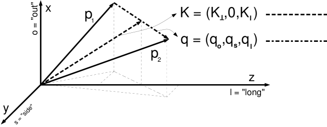
3.1.1 Azimuthally symmetric collisions

For central collisions, $\leavevmode\mathchoice{\hbox{\rm tensysevensyfivesy\boldmath{$\displaystyle b$}}}{\hbox{\rm tensysevensyfivesy\boldmath{$\textstyle b$}}}{\hbox{\rm tensysevensyfivesy\boldmath{$\scriptstyle b$}}}{\hbox{\rm tensysevensyfivesy\boldmath{$\scriptscriptstyle b$}}}=0$, the collision region is azimuthally symmetric, and the emission function and correlator are $\Phi$-independent. In the osl-system, this $\Phi$-invariance results in a reflection symmetry with respect to the side-direction [40]:

$\displaystyle S_{\rm lab}(x;K_{\perp},\Phi,K_{l})=S_{\rm lab}(x;K_{\perp},\Phi+\delta\Phi,K_{l})$
$\displaystyle\Longleftrightarrow S_{\rm osl}(x,y,z,t;K_{\perp},K_{l})=S_{\rm osl}(x,-y,z,t;K_{\perp},K_{l})\,.$ (3.9)

We follow common practice in dropping now the subscript osl. Whenever azimuthal symmetry is assumed, the emission function $S(x,K)$ is specified in the osl-system.

Due to the $y\to-y$ reflection symmetry of the emission function, $\overline{y}=\langle y\rangle=0$ and the three space-time variances $\langle\tilde{x}_{\mu}\tilde{x}_{\nu}\rangle(\leavevmode\mathchoice{\hbox{\rm tensysevensyfivesy\boldmath{$\displaystyle K$}}}{\hbox{\rm tensysevensyfivesy\boldmath{$\textstyle K$}}}{\hbox{\rm tensysevensyfivesy\boldmath{$\scriptstyle K$}}}{\hbox{\rm tensysevensyfivesy\boldmath{$\scriptscriptstyle K$}}})$ linear in $\tilde{y}$ vanish. The symmetric tensor $B_{\mu\nu}(\leavevmode\mathchoice{\hbox{\rm tensysevensyfivesy\boldmath{$\displaystyle K$}}}{\hbox{\rm tensysevensyfivesy\boldmath{$\textstyle K$}}}{\hbox{\rm tensysevensyfivesy\boldmath{$\scriptstyle K$}}}{\hbox{\rm tensysevensyfivesy\boldmath{$\scriptscriptstyle K$}}})$ then has only seven non-vanishing independent components. These combine to four non-vanishing HBT-radius parameters $R_{ij}^{2}(\leavevmode\mathchoice{\hbox{\rm tensysevensyfivesy\boldmath{$\displaystyle K$}}}{\hbox{\rm tensysevensyfivesy\boldmath{$\textstyle K$}}}{\hbox{\rm tensysevensyfivesy\boldmath{$\scriptstyle K$}}}{\hbox{\rm tensysevensyfivesy\boldmath{$\scriptscriptstyle K$}}})$ which characterize the Gaussian ansatz (1.5) for the correlator [41, 89]:

$\displaystyle R_{s}^{2}(\leavevmode\mathchoice{\hbox{\rm tensysevensyfivesy\boldmath{$\displaystyle K$}}}{\hbox{\rm tensysevensyfivesy\boldmath{$\textstyle K$}}}{\hbox{\rm tensysevensyfivesy\boldmath{$\scriptstyle K$}}}{\hbox{\rm tensysevensyfivesy\boldmath{$\scriptscriptstyle K$}}})$ $\displaystyle=$ $\displaystyle\langle\tilde{y}^{2}\rangle(\leavevmode\mathchoice{\hbox{\rm tensysevensyfivesy\boldmath{$\displaystyle K$}}}{\hbox{\rm tensysevensyfivesy\boldmath{$\textstyle K$}}}{\hbox{\rm tensysevensyfivesy\boldmath{$\scriptstyle K$}}}{\hbox{\rm tensysevensyfivesy\boldmath{$\scriptscriptstyle K$}}})\,,$ (3.10)
$\displaystyle R_{o}^{2}(\leavevmode\mathchoice{\hbox{\rm tensysevensyfivesy\boldmath{$\displaystyle K$}}}{\hbox{\rm tensysevensyfivesy\boldmath{$\textstyle K$}}}{\hbox{\rm tensysevensyfivesy\boldmath{$\scriptstyle K$}}}{\hbox{\rm tensysevensyfivesy\boldmath{$\scriptscriptstyle K$}}})$ $\displaystyle=$ $\displaystyle\langle(\tilde{x}-\beta_{\perp}\tilde{t})^{2}\rangle(\leavevmode\mathchoice{\hbox{\rm tensysevensyfivesy\boldmath{$\displaystyle K$}}}{\hbox{\rm tensysevensyfivesy\boldmath{$\textstyle K$}}}{\hbox{\rm tensysevensyfivesy\boldmath{$\scriptstyle K$}}}{\hbox{\rm tensysevensyfivesy\boldmath{$\scriptscriptstyle K$}}})\,,$ (3.11)
$\displaystyle R_{l}^{2}(\leavevmode\mathchoice{\hbox{\rm tensysevensyfivesy\boldmath{$\displaystyle K$}}}{\hbox{\rm tensysevensyfivesy\boldmath{$\textstyle K$}}}{\hbox{\rm tensysevensyfivesy\boldmath{$\scriptstyle K$}}}{\hbox{\rm tensysevensyfivesy\boldmath{$\scriptscriptstyle K$}}})$ $\displaystyle=$ $\displaystyle\langle(\tilde{z}-\beta_{l}\tilde{t})^{2}\rangle(\leavevmode\mathchoice{\hbox{\rm tensysevensyfivesy\boldmath{$\displaystyle K$}}}{\hbox{\rm tensysevensyfivesy\boldmath{$\textstyle K$}}}{\hbox{\rm tensysevensyfivesy\boldmath{$\scriptstyle K$}}}{\hbox{\rm tensysevensyfivesy\boldmath{$\scriptscriptstyle K$}}})\,,$ (3.12)
$\displaystyle R_{ol}^{2}(\leavevmode\mathchoice{\hbox{\rm tensysevensyfivesy\boldmath{$\displaystyle K$}}}{\hbox{\rm tensysevensyfivesy\boldmath{$\textstyle K$}}}{\hbox{\rm tensysevensyfivesy\boldmath{$\scriptstyle K$}}}{\hbox{\rm tensysevensyfivesy\boldmath{$\scriptscriptstyle K$}}})$ $\displaystyle=$ $\displaystyle\langle(\tilde{x}-\beta_{\perp}\tilde{t})(\tilde{z}-\beta_{l}\tilde{t})\rangle(\leavevmode\mathchoice{\hbox{\rm tensysevensyfivesy\boldmath{$\displaystyle K$}}}{\hbox{\rm tensysevensyfivesy\boldmath{$\textstyle K$}}}{\hbox{\rm tensysevensyfivesy\boldmath{$\scriptstyle K$}}}{\hbox{\rm tensysevensyfivesy\boldmath{$\scriptscriptstyle K$}}})\,,$ (3.13)
$\displaystyle R_{os}^{2}(\leavevmode\mathchoice{\hbox{\rm tensysevensyfivesy\boldmath{$\displaystyle K$}}}{\hbox{\rm tensysevensyfivesy\boldmath{$\textstyle K$}}}{\hbox{\rm tensysevensyfivesy\boldmath{$\scriptstyle K$}}}{\hbox{\rm tensysevensyfivesy\boldmath{$\scriptscriptstyle K$}}})$ $\displaystyle=$ $\displaystyle 0\,,$ (3.14)
$\displaystyle R_{sl}^{2}(\leavevmode\mathchoice{\hbox{\rm tensysevensyfivesy\boldmath{$\displaystyle K$}}}{\hbox{\rm tensysevensyfivesy\boldmath{$\textstyle K$}}}{\hbox{\rm tensysevensyfivesy\boldmath{$\scriptstyle K$}}}{\hbox{\rm tensysevensyfivesy\boldmath{$\scriptscriptstyle K$}}})$ $\displaystyle=$ $\displaystyle 0\,.$ (3.15)

Obviously, the more symmetries are satisfied by the emission function, the simpler are the expressions obtained for the HBT radius parameters. In this context we mention the case of a longitudinally boost-invariant source showing Bjorken scaling. Though not strictly satisfied by the finite sources created in heavy-ion collisions, this can provide a simple intuitive picture of the collision dynamics near mid-rapidity. Longitudinal boost-invariance implies a $\tilde{z}\to-\tilde{z}$ reflection symmetry of the emission function. Thus, in addition to the space-time variances linear in $\tilde{y}$, now also those linear in $\tilde{z}$ vanish, and one is left with only 5 non-vanishing independent components of $B_{\mu\nu}(\leavevmode\mathchoice{\hbox{\rm tensysevensyfivesy\boldmath{$\displaystyle K$}}}{\hbox{\rm tensysevensyfivesy\boldmath{$\textstyle K$}}}{\hbox{\rm tensysevensyfivesy\boldmath{$\scriptstyle K$}}}{\hbox{\rm tensysevensyfivesy\boldmath{$\scriptscriptstyle K$}}})$. In the longitudinally comoving system (LCMS), where $\beta_{l}=0$, this leads to the further simplications

$\displaystyle\qquad\qquad\qquad R_{l}^{2}(\leavevmode\mathchoice{\hbox{\rm tensysevensyfivesy\boldmath{$\displaystyle K$}}}{\hbox{\rm tensysevensyfivesy\boldmath{$\textstyle K$}}}{\hbox{\rm tensysevensyfivesy\boldmath{$\scriptstyle K$}}}{\hbox{\rm tensysevensyfivesy\boldmath{$\scriptscriptstyle K$}}})=\langle\tilde{z}^{2}\rangle(\leavevmode\mathchoice{\hbox{\rm tensysevensyfivesy\boldmath{$\displaystyle K$}}}{\hbox{\rm tensysevensyfivesy\boldmath{$\textstyle K$}}}{\hbox{\rm tensysevensyfivesy\boldmath{$\scriptstyle K$}}}{\hbox{\rm tensysevensyfivesy\boldmath{$\scriptscriptstyle K$}}})\,,$ (3.16)
$\displaystyle\qquad\qquad\qquad R_{ol}^{2}(\leavevmode\mathchoice{\hbox{\rm tensysevensyfivesy\boldmath{$\displaystyle K$}}}{\hbox{\rm tensysevensyfivesy\boldmath{$\textstyle K$}}}{\hbox{\rm tensysevensyfivesy\boldmath{$\scriptstyle K$}}}{\hbox{\rm tensysevensyfivesy\boldmath{$\scriptscriptstyle K$}}})=0\,,$ (3.17)
for longitudinally boost-invariant sources in the LCMS.

The general relation between the symmetries of the system, the number of its independent non-vanishing space-time variances, and the number of non-vanishing observable HBT parameters is summarized in the following table:
symmetry $B_{\mu\nu}(\leavevmode\mathchoice{\hbox{\rm tensysevensyfivesy\boldmath{$\displaystyle K$}}}{\hbox{\rm tensysevensyfivesy\boldmath{$\textstyle K$}}}{\hbox{\rm tensysevensyfivesy\boldmath{$\scriptstyle K$}}}{\hbox{\rm tensysevensyfivesy\boldmath{$\scriptscriptstyle K$}}})$ $R_{ij}(\leavevmode\mathchoice{\hbox{\rm tensysevensyfivesy\boldmath{$\displaystyle K$}}}{\hbox{\rm tensysevensyfivesy\boldmath{$\textstyle K$}}}{\hbox{\rm tensysevensyfivesy\boldmath{$\scriptstyle K$}}}{\hbox{\rm tensysevensyfivesy\boldmath{$\scriptscriptstyle K$}}})$ none 10 indep. fcts. 6 indep. fcts. of $K_{\perp}$, $\phi$, $Y$ of $K_{\perp}$, $\phi$, $Y$ azimuthal 7 indep. fcts. 4 indep. fcts. of $K_{\perp}$, $Y$ of $K_{\perp}$, $Y$ azimuthal 5 indep. fcts. 3 indep. fcts. + long. boostinv. of $K_{\perp}$ of $K_{\perp}$ in the LCMS
In all cases, there are more independent space-time variances $\langle x_{\mu}x_{\nu}\rangle(\leavevmode\mathchoice{\hbox{\rm tensysevensyfivesy\boldmath{$\displaystyle K$}}}{\hbox{\rm tensysevensyfivesy\boldmath{$\textstyle K$}}}{\hbox{\rm tensysevensyfivesy\boldmath{$\scriptstyle K$}}}{\hbox{\rm tensysevensyfivesy\boldmath{$\scriptscriptstyle K$}}})$ than experimental observables. This arises from the mass-shell constraint (2.27) which leads to a mixing of spatial and temporal variances in the observable HBT parameters. One of the most important questions is therefore which other properties of the expanding system can be exploited to further disentangle spatial and temporal information about the emission function.

For this, we note that independent of the particular emission function, no direction is distinguished in the transverse plane for $K_{\perp}=0$. The out- and side-components of all observables coincide in this kinematical limit. For the space-time variances, this implies

$\displaystyle\langle\tilde{x}^{2}\rangle\Big{|}_{K_{\perp}=0}$ $\displaystyle=$ $\displaystyle\langle\tilde{y}^{2}\rangle\Big{|}_{K_{\perp}=0}\,,$ (3.18)
$\displaystyle\langle\tilde{z}\tilde{x}\rangle\Big{|}_{K_{\perp}=0}$ $\displaystyle=$ $\displaystyle\langle\tilde{t}\tilde{x}\rangle\Big{|}_{K_{\perp}=0}=0\,.$ (3.19)

As long as the limit $K_{\perp}\to 0$ of the emission function $S(x,K)$ results in an azimuthally symmetric expression (an exception is the class of opaque source models discussed in section 5.1.2), the above relations between the space-time variances at $K_{\perp}=0$ imply that the HBT radius parameters satisfy

$\displaystyle\lim_{K_{\perp}\to 0}R_{o}^{2}(\leavevmode\mathchoice{\hbox{\rm tensysevensyfivesy\boldmath{$\displaystyle K$}}}{\hbox{\rm tensysevensyfivesy\boldmath{$\textstyle K$}}}{\hbox{\rm tensysevensyfivesy\boldmath{$\scriptstyle K$}}}{\hbox{\rm tensysevensyfivesy\boldmath{$\scriptscriptstyle K$}}})$ $\displaystyle=$ $\displaystyle\lim_{K_{\perp}\to 0}R_{s}^{2}(\leavevmode\mathchoice{\hbox{\rm tensysevensyfivesy\boldmath{$\displaystyle K$}}}{\hbox{\rm tensysevensyfivesy\boldmath{$\textstyle K$}}}{\hbox{\rm tensysevensyfivesy\boldmath{$\scriptstyle K$}}}{\hbox{\rm tensysevensyfivesy\boldmath{$\scriptscriptstyle K$}}})\,,$ (3.20)
$\displaystyle\lim_{K_{\perp}\to 0}R_{ol}^{2}(\leavevmode\mathchoice{\hbox{\rm tensysevensyfivesy\boldmath{$\displaystyle K$}}}{\hbox{\rm tensysevensyfivesy\boldmath{$\textstyle K$}}}{\hbox{\rm tensysevensyfivesy\boldmath{$\scriptstyle K$}}}{\hbox{\rm tensysevensyfivesy\boldmath{$\scriptscriptstyle K$}}})$ $\displaystyle=$ $\displaystyle 0\,.$ (3.21)

In phenomenological HBT analyses one very often exploits these relations by distinguishing between an implicit tensysevensyfivesy$\textstyle K$-dependence (due to the tensysevensyfivesy$\textstyle K$-dependence of the space-time variances) and an explicit one (resulting from the mass-shell constraint $q^{0}=\leavevmode\mathchoice{\hbox{\rm tensysevensyfivesy\boldmath{$\displaystyle q$}}}{\hbox{\rm tensysevensyfivesy\boldmath{$\textstyle q$}}}{\hbox{\rm tensysevensyfivesy\boldmath{$\scriptstyle q$}}}{\hbox{\rm tensysevensyfivesy\boldmath{$\scriptscriptstyle q$}}}\cdot\leavevmode\mathchoice{\hbox{\rm tensysevensyfivesy\boldmath{$\displaystyle K$}}}{\hbox{\rm tensysevensyfivesy\boldmath{$\textstyle K$}}}{\hbox{\rm tensysevensyfivesy\boldmath{$\scriptstyle K$}}}{\hbox{\rm tensysevensyfivesy\boldmath{$\scriptscriptstyle K$}}}/K^{0}$). If the emission function features no position-momentum correlation, then all space-time variances are tensysevensyfivesy$\textstyle K$-independent and Eqs. (3.18/3.19) hold independently of tensysevensyfivesy$\textstyle K$. The difference between $R_{o}^{2}(\leavevmode\mathchoice{\hbox{\rm tensysevensyfivesy\boldmath{$\displaystyle K$}}}{\hbox{\rm tensysevensyfivesy\boldmath{$\textstyle K$}}}{\hbox{\rm tensysevensyfivesy\boldmath{$\scriptstyle K$}}}{\hbox{\rm tensysevensyfivesy\boldmath{$\scriptscriptstyle K$}}})$ and $R_{s}^{2}(\leavevmode\mathchoice{\hbox{\rm tensysevensyfivesy\boldmath{$\displaystyle K$}}}{\hbox{\rm tensysevensyfivesy\boldmath{$\textstyle K$}}}{\hbox{\rm tensysevensyfivesy\boldmath{$\scriptstyle K$}}}{\hbox{\rm tensysevensyfivesy\boldmath{$\scriptscriptstyle K$}}})$ at non-zero tensysevensyfivesy$\textstyle K$ is then only due to the explicit tensysevensyfivesy$\textstyle K$-dependence in (3.10/3.11), i.e. the term $\beta_{\perp}^{2}\langle\tilde{t}^{2}\rangle$. This implies that the explicit tensysevensyfivesy$\textstyle K$-dependence dominates if the emission duration is sufficiently large [138] or if the position-momentum correlations in the source are sufficiently weak [26, 127],

$$R_{o}^{2}(\leavevmode\mathchoice{\hbox{\rm tensysevensyfivesy\boldmath{$\displaystyle K$}}}{\hbox{\rm tensysevensyfivesy\boldmath{$\textstyle K$}}}{\hbox{\rm tensysevensyfivesy\boldmath{$\scriptstyle K$}}}{\hbox{\rm tensysevensyfivesy\boldmath{$\scriptscriptstyle K$}}})-R_{s}^{2}(\leavevmode\mathchoice{\hbox{\rm tensysevensyfivesy\boldmath{$\displaystyle K$}}}{\hbox{\rm tensysevensyfivesy\boldmath{$\textstyle K$}}}{\hbox{\rm tensysevensyfivesy\boldmath{$\scriptstyle K$}}}{\hbox{\rm tensysevensyfivesy\boldmath{$\scriptscriptstyle K$}}})\approx\beta_{\perp}^{2}\langle\tilde{t}^{2}\rangle\,.$$ (3.22)

In this case, the difference between these two HBT radius parameters gives direct access to the average emission duration $\langle\tilde{t}^{2}\rangle$ of the source and allows to partially disentangle the spatial and temporal information contained in (3.10)-(3.15).

The gives rise to the following simple interpretation of the HBT radius parameters from the Cartesian parametrization: $R_{s}$ measures the width of the emission region in the side direction, and $R_{o}$ measures the corresponding width in the out direction plus a contribution from the emission duration which can be extracted according to (3.22) under the assumption of a weak $K_{\perp}$-dependence of the emission function. The longitudinal radius $R_{l}$ finally describes the longitudinal extension of the region of homogeneity in the LCMS where $\beta_{l}=0$. No easy intuitive interpretation exists for the out-longitudinal radius parameter $R_{ol}^{2}$. It is perhaps best understood in terms of the linear correlation coefficient [144]

$$\rho_{ol}(\leavevmode\mathchoice{\hbox{\rm tensysevensyfivesy\boldmath{$\displaystyle K$}}}{\hbox{\rm tensysevensyfivesy\boldmath{$\textstyle K$}}}{\hbox{\rm tensysevensyfivesy\boldmath{$\scriptstyle K$}}}{\hbox{\rm tensysevensyfivesy\boldmath{$\scriptscriptstyle K$}}})=-{R_{ol}^{2}(\leavevmode\mathchoice{\hbox{\rm tensysevensyfivesy\boldmath{$\displaystyle K$}}}{\hbox{\rm tensysevensyfivesy\boldmath{$\textstyle K$}}}{\hbox{\rm tensysevensyfivesy\boldmath{$\scriptstyle K$}}}{\hbox{\rm tensysevensyfivesy\boldmath{$\scriptscriptstyle K$}}})\over R_{o}(\leavevmode\mathchoice{\hbox{\rm tensysevensyfivesy\boldmath{$\displaystyle K$}}}{\hbox{\rm tensysevensyfivesy\boldmath{$\textstyle K$}}}{\hbox{\rm tensysevensyfivesy\boldmath{$\scriptstyle K$}}}{\hbox{\rm tensysevensyfivesy\boldmath{$\scriptscriptstyle K$}}})\,R_{l}(\leavevmode\mathchoice{\hbox{\rm tensysevensyfivesy\boldmath{$\displaystyle K$}}}{\hbox{\rm tensysevensyfivesy\boldmath{$\textstyle K$}}}{\hbox{\rm tensysevensyfivesy\boldmath{$\scriptstyle K$}}}{\hbox{\rm tensysevensyfivesy\boldmath{$\scriptscriptstyle K$}}})}\,,$$ (3.23)

which can be positive or negative but is bounded by $|\rho_{ol}(\leavevmode\mathchoice{\hbox{\rm tensysevensyfivesy\boldmath{$\displaystyle K$}}}{\hbox{\rm tensysevensyfivesy\boldmath{$\textstyle K$}}}{\hbox{\rm tensysevensyfivesy\boldmath{$\scriptstyle K$}}}{\hbox{\rm tensysevensyfivesy\boldmath{$\scriptscriptstyle K$}}})|\leq 1$ due to the Cauchy-Schwarz inequality. This coefficient was shown [144] to be of kinematical origin and useful for the interpretation of the longitudinal momentum distributions. We shall see in section 3.2 that $R_{ol}$ plays a crucial role in the determination of the longitudinal velocity of the emitting source volume element.

3.1.2 Collisions with finite impact parameter

If the azimuthal symmetry of the particle emitting source is broken, then the transverse one-particle spectrum depends on the azimuthal direction of the emitted particles. This can be quantified in terms of the harmonic coefficients $v_{n}(p_{t},y)$[116, 117, 165]

$\displaystyle E{dN\over d^{3}p}$ $\displaystyle=$ $\displaystyle E{dN\over p_{t}\,dp_{t}\,dy\,d\phi}=\int d^{4}x\,S(x,p)$
$\displaystyle=$ $\displaystyle{E\over 2\pi}{d^{2}N\over p_{t}\,dp_{t}\,dy}\left[1+2\sum_{n=1}^{\infty}v_{n}(p_{t},y)\,\cos n(\phi-\psi_{R})\right]\,.$

The size and momentum dependence of the lowest of these harmonic coefficients has been analyzed experimentally at both AGS and CERN SPS energies [15, 16, 118, 124]. This allows to determine the orientation of the reaction plane for semiperipheral collisions event by event with an uncertainty of less than 30 [165, 124]. Several attempts to extend this azimuthally sensitive analysis to two-particle correlation functions exist [167, 56, 175]. The correlation measurements depend on the azimuthal direction $\Phi$ of the pair momentum, see (3.8), and hence allow to provide additional azimuthally sensitive information. The corresponding Gaussian radius parameters can be written formally in terms of space-time variances which are rotated via ${\cal D}_{\Phi}$ from the impact parameter fixed to the osl coordinate system [175]

$\displaystyle R_{ij}^{2}(\leavevmode\mathchoice{\hbox{\rm tensysevensyfivesy\boldmath{$\displaystyle K$}}}{\hbox{\rm tensysevensyfivesy\boldmath{$\textstyle K$}}}{\hbox{\rm tensysevensyfivesy\boldmath{$\scriptstyle K$}}}{\hbox{\rm tensysevensyfivesy\boldmath{$\scriptscriptstyle K$}}})=\left\langle\left[\left({\cal D}_{\Phi}\tilde{x}\right)_{i}-\left({\cal D}_{\Phi}\leavevmode\mathchoice{\hbox{\rm tensysevensyfivesy\boldmath{$\displaystyle\beta$}}}{\hbox{\rm tensysevensyfivesy\boldmath{$\textstyle\beta$}}}{\hbox{\rm tensysevensyfivesy\boldmath{$\scriptstyle\beta$}}}{\hbox{\rm tensysevensyfivesy\boldmath{$\scriptscriptstyle\beta$}}}\right)_{i}\tilde{t}\right]\left[\left({\cal D}_{\Phi}\tilde{x}\right)_{j}-\left({\cal D}_{\Phi}\leavevmode\mathchoice{\hbox{\rm tensysevensyfivesy\boldmath{$\displaystyle\beta$}}}{\hbox{\rm tensysevensyfivesy\boldmath{$\textstyle\beta$}}}{\hbox{\rm tensysevensyfivesy\boldmath{$\scriptstyle\beta$}}}{\hbox{\rm tensysevensyfivesy\boldmath{$\scriptscriptstyle\beta$}}}\right)_{j}\tilde{t}\right]\right\rangle\,,$
$\displaystyle\left({\cal D}_{\Phi}\leavevmode\mathchoice{\hbox{\rm tensysevensyfivesy\boldmath{$\displaystyle\beta$}}}{\hbox{\rm tensysevensyfivesy\boldmath{$\textstyle\beta$}}}{\hbox{\rm tensysevensyfivesy\boldmath{$\scriptstyle\beta$}}}{\hbox{\rm tensysevensyfivesy\boldmath{$\scriptscriptstyle\beta$}}}\right)=\left(\beta_{\perp},\,0,\,\beta_{l}\right)\,.$ (3.25)

We here differ from the notation adopted in the rest of this review: the coordinates $x$, $y$ and $z$ are here given in the impact-parameter fixed system, not the osl one. As for the azimuthally symmetric case, the HBT radius parameters show implict and explicit tensysevensyfivesy$\textstyle K$-dependences. Their $\Phi$-dependence thus has two different origins [167, 175]:

$\displaystyle R_{s}^{2}(K_{\perp},\Phi,Y)=\langle\tilde{x}^{2}\rangle\sin^{2}\Phi+\langle\tilde{y}^{2}\rangle\cos^{2}\Phi-\langle\tilde{x}\tilde{y}\rangle\sin 2\Phi\,,$
$\displaystyle R_{o}^{2}(K_{\perp},\Phi,Y)=\langle\tilde{x}^{2}\rangle\cos^{2}\Phi+\langle\tilde{y}^{2}\rangle\sin^{2}\Phi+\beta_{\perp}^{2}\langle\tilde{t}^{2}\rangle$
$\displaystyle\qquad\qquad-2\beta_{\perp}\langle\tilde{t}\tilde{x}\rangle\cos\Phi-2\beta_{\perp}\langle\tilde{t}\tilde{y}\rangle\sin\Phi+\langle\tilde{x}\tilde{y}\rangle\sin 2\Phi\,,$
$\displaystyle R_{os}^{2}(K_{\perp},\Phi,Y)=\langle\tilde{x}\tilde{y}\rangle\cos 2\Phi+\textstyle{1\over 2}\sin 2\Phi(\langle\tilde{y}^{2}\rangle-\langle\tilde{x}^{2}\rangle)$
$\displaystyle\qquad\qquad+\beta_{\perp}\langle\tilde{t}\tilde{x}\rangle\sin\Phi-\beta_{\perp}\langle\tilde{t}\tilde{y}\rangle\cos\Phi\,,$
$\displaystyle R_{l}^{2}(K_{\perp},\Phi,Y)=\langle(\tilde{z}-\beta_{l}\tilde{t})^{2}\rangle\,,$
$\displaystyle R_{ol}^{2}(K_{\perp},\Phi,Y)=\langle(\tilde{z}-\beta_{l}\tilde{t})(\tilde{x}\cos\Phi+\tilde{y}\sin\Phi-\beta_{\perp}\tilde{t})\rangle\,,$
$\displaystyle R_{sl}^{2}(K_{\perp},\Phi,Y)=\langle(\tilde{z}-\beta_{l}\tilde{t})(\tilde{y}\cos\Phi-\tilde{x}\sin\Phi)\rangle\,.$ (3.26)

The explicit $\Phi$-dependence denoted here is a purely geometrical consequence of rotating the $x$-axis from the direction of tensysevensyfivesy$\textstyle b$ to the direction of $\leavevmode\mathchoice{\hbox{\rm tensysevensyfivesy\boldmath{$\displaystyle K$}}}{\hbox{\rm tensysevensyfivesy\boldmath{$\textstyle K$}}}{\hbox{\rm tensysevensyfivesy\boldmath{$\scriptstyle K$}}}{\hbox{\rm tensysevensyfivesy\boldmath{$\scriptscriptstyle K$}}}_{\perp}$. In addition, there is an implicit $\Phi$-dependence of the space-time variances, $\langle\tilde{x}_{\mu}\tilde{x}_{\nu}\rangle$ $=\langle\tilde{x}_{\mu}\tilde{x}_{\nu}\rangle(K_{\perp},\Phi,Y)$. This $\Phi$-dependence characterizes the dynamical correlations between the size of the effective emission region (“region of homogeneity”) and the azimuthal direction in which particles are emitted. Both implicit and explicit $\Phi$-dependences are mixed in the harmonic coefficients

$\displaystyle{R_{ij,m}^{c}}^{2}$ $\displaystyle=$ $\displaystyle{1\over 2\pi}\int_{-\pi}^{\pi}R_{ij}^{2}\,\cos(m\Phi)\,d\Phi\,,$ (3.27)
$\displaystyle{R_{ij,m}^{s}}^{2}$ $\displaystyle=$ $\displaystyle{1\over 2\pi}\int_{-\pi}^{\pi}R_{ij}^{2}\,\sin(m\Phi)\,d\Phi\,.$ (3.28)

In models in which elliptic deformations dominate and higher than second order harmonic coefficients can be neglected, these coefficients satisfy the relations [175]

$\displaystyle\alpha_{1}(K_{\perp},Y)\approx{R_{s,1}^{c}}^{2}\approx\textstyle{1\over 3}{R_{o,1}^{c}}^{2}\approx-{R_{os,1}^{s}}^{2}\,,$ (3.29)
$\displaystyle\alpha_{2}(K_{\perp},Y)\approx{R_{o,2}^{c}}^{2}\approx-{R_{s,2}^{c}}^{2}\approx-{R_{os,2}^{s}}^{2}\,.$ (3.30)

The anisotropy parameter $\alpha_{1}$ vanishes in the absence of position-momentum correlations in the source and thus characterizes dynamical anisotropies. On the other hand, $\alpha_{2}$ characterizes the elliptical shape of the emission region. A violation of the relations (3.29)-(3.30) would rule out a large class of model scenarios considered to be consistent with the present knowledge about the space-time evolution of the collision process.

Constraints of the type (3.29/3.30) on the harmonic coefficients lead to a minimal azimuthally sensitive parametrization of the two-particle correlator [175]:

$\displaystyle C_{\psi_{R}}(\leavevmode\mathchoice{\hbox{\rm tensysevensyfivesy\boldmath{$\displaystyle q$}}}{\hbox{\rm tensysevensyfivesy\boldmath{$\textstyle q$}}}{\hbox{\rm tensysevensyfivesy\boldmath{$\scriptstyle q$}}}{\hbox{\rm tensysevensyfivesy\boldmath{$\scriptscriptstyle q$}}},\leavevmode\mathchoice{\hbox{\rm tensysevensyfivesy\boldmath{$\displaystyle K$}}}{\hbox{\rm tensysevensyfivesy\boldmath{$\textstyle K$}}}{\hbox{\rm tensysevensyfivesy\boldmath{$\scriptstyle K$}}}{\hbox{\rm tensysevensyfivesy\boldmath{$\scriptscriptstyle K$}}})$ $\displaystyle\approx$ $\displaystyle 1+\lambda(\leavevmode\mathchoice{\hbox{\rm tensysevensyfivesy\boldmath{$\displaystyle K$}}}{\hbox{\rm tensysevensyfivesy\boldmath{$\textstyle K$}}}{\hbox{\rm tensysevensyfivesy\boldmath{$\scriptstyle K$}}}{\hbox{\rm tensysevensyfivesy\boldmath{$\scriptscriptstyle K$}}})\,\,C_{sym}(\leavevmode\mathchoice{\hbox{\rm tensysevensyfivesy\boldmath{$\displaystyle q$}}}{\hbox{\rm tensysevensyfivesy\boldmath{$\textstyle q$}}}{\hbox{\rm tensysevensyfivesy\boldmath{$\scriptstyle q$}}}{\hbox{\rm tensysevensyfivesy\boldmath{$\scriptscriptstyle q$}}},\leavevmode\mathchoice{\hbox{\rm tensysevensyfivesy\boldmath{$\displaystyle K$}}}{\hbox{\rm tensysevensyfivesy\boldmath{$\textstyle K$}}}{\hbox{\rm tensysevensyfivesy\boldmath{$\scriptstyle K$}}}{\hbox{\rm tensysevensyfivesy\boldmath{$\scriptscriptstyle K$}}})\,C_{1}(\leavevmode\mathchoice{\hbox{\rm tensysevensyfivesy\boldmath{$\displaystyle q$}}}{\hbox{\rm tensysevensyfivesy\boldmath{$\textstyle q$}}}{\hbox{\rm tensysevensyfivesy\boldmath{$\scriptstyle q$}}}{\hbox{\rm tensysevensyfivesy\boldmath{$\scriptscriptstyle q$}}},\leavevmode\mathchoice{\hbox{\rm tensysevensyfivesy\boldmath{$\displaystyle K$}}}{\hbox{\rm tensysevensyfivesy\boldmath{$\textstyle K$}}}{\hbox{\rm tensysevensyfivesy\boldmath{$\scriptstyle K$}}}{\hbox{\rm tensysevensyfivesy\boldmath{$\scriptscriptstyle K$}}},\psi_{R})$ (3.31)
$\displaystyle\qquad\qquad\times C_{2}(\leavevmode\mathchoice{\hbox{\rm tensysevensyfivesy\boldmath{$\displaystyle q$}}}{\hbox{\rm tensysevensyfivesy\boldmath{$\textstyle q$}}}{\hbox{\rm tensysevensyfivesy\boldmath{$\scriptstyle q$}}}{\hbox{\rm tensysevensyfivesy\boldmath{$\scriptscriptstyle q$}}},\leavevmode\mathchoice{\hbox{\rm tensysevensyfivesy\boldmath{$\displaystyle K$}}}{\hbox{\rm tensysevensyfivesy\boldmath{$\textstyle K$}}}{\hbox{\rm tensysevensyfivesy\boldmath{$\scriptstyle K$}}}{\hbox{\rm tensysevensyfivesy\boldmath{$\scriptscriptstyle K$}}},\psi_{R})\,,$
$\displaystyle C_{sym}(\leavevmode\mathchoice{\hbox{\rm tensysevensyfivesy\boldmath{$\displaystyle q$}}}{\hbox{\rm tensysevensyfivesy\boldmath{$\textstyle q$}}}{\hbox{\rm tensysevensyfivesy\boldmath{$\scriptstyle q$}}}{\hbox{\rm tensysevensyfivesy\boldmath{$\scriptscriptstyle q$}}},\leavevmode\mathchoice{\hbox{\rm tensysevensyfivesy\boldmath{$\displaystyle K$}}}{\hbox{\rm tensysevensyfivesy\boldmath{$\textstyle K$}}}{\hbox{\rm tensysevensyfivesy\boldmath{$\scriptstyle K$}}}{\hbox{\rm tensysevensyfivesy\boldmath{$\scriptscriptstyle K$}}})$ $\displaystyle=$ $\displaystyle\exp[-{R_{o,0}}^{2}\,q_{o}^{2}-{R_{s,0}}^{2}\,q_{s}^{2}$ (3.32)
$\displaystyle\qquad-{R_{l,0}}^{2}\,q_{l}^{2}-2\,{R_{ol,0}}^{2}\,q_{o}q_{l}]\,,$
$\displaystyle C_{1}(\leavevmode\mathchoice{\hbox{\rm tensysevensyfivesy\boldmath{$\displaystyle q$}}}{\hbox{\rm tensysevensyfivesy\boldmath{$\textstyle q$}}}{\hbox{\rm tensysevensyfivesy\boldmath{$\scriptstyle q$}}}{\hbox{\rm tensysevensyfivesy\boldmath{$\scriptscriptstyle q$}}},\leavevmode\mathchoice{\hbox{\rm tensysevensyfivesy\boldmath{$\displaystyle K$}}}{\hbox{\rm tensysevensyfivesy\boldmath{$\textstyle K$}}}{\hbox{\rm tensysevensyfivesy\boldmath{$\scriptstyle K$}}}{\hbox{\rm tensysevensyfivesy\boldmath{$\scriptscriptstyle K$}}},\psi_{R})$ $\displaystyle=$ $\displaystyle\exp\big{[}-\alpha_{1}\,(3\,q_{o}^{2}+q_{s}^{2})\,\cos(\Phi-\psi_{R})\,$ (3.33)
$\displaystyle\qquad+2\alpha_{1}\,q_{o}q_{s}\sin(\Phi-\psi_{R})\big{]}\,,$
$\displaystyle C_{2}(\leavevmode\mathchoice{\hbox{\rm tensysevensyfivesy\boldmath{$\displaystyle q$}}}{\hbox{\rm tensysevensyfivesy\boldmath{$\textstyle q$}}}{\hbox{\rm tensysevensyfivesy\boldmath{$\scriptstyle q$}}}{\hbox{\rm tensysevensyfivesy\boldmath{$\scriptscriptstyle q$}}},\leavevmode\mathchoice{\hbox{\rm tensysevensyfivesy\boldmath{$\displaystyle K$}}}{\hbox{\rm tensysevensyfivesy\boldmath{$\textstyle K$}}}{\hbox{\rm tensysevensyfivesy\boldmath{$\scriptstyle K$}}}{\hbox{\rm tensysevensyfivesy\boldmath{$\scriptscriptstyle K$}}},\psi_{R})$ $\displaystyle=$ $\displaystyle\exp\big{[}-\alpha_{2}(q_{o}^{2}-q_{s}^{2})\cos 2(\Phi-\psi_{R})$ (3.34)
$\displaystyle\qquad+2\,\alpha_{2}q_{o}q_{s}\sin 2(\Phi-\psi_{R})\big{]}\,.$

In addition to the azimuthally symmetric part (3.32) which coincides with the Cartesian parametrization, this Gaussian ansatz involves only two additional, azimuthally sensitive fit parameters.

Refer to caption


Figure 3.2: The HBT anisotropy parameters $\langle\alpha_{i}\rangle$ as a function of the parameter $\bar{\xi}$ which characterizes the event-by-event reconstruction uncertainty in the orientation of the reaction plane. The parameters $\langle\alpha_{1}\rangle$, $\langle\alpha_{2}\rangle$ are determined by fitting (3.31) to an event sample (3.36) of correlators whose reconstructed reaction planes fluctuate around the true impact parameter with the probability distribution (3.35). The value $\bar{\xi}=2$ corresponds to a reconstruction uncertainty of approximately $30^{\circ}$.

The major difficulty in determining the harmonic coefficients (3.27/3.28) from experiment is that they are expected to be statistically meaningful only for relatively large event samples while their extraction is conditional upon the eventwise reconstruction of the reaction plane. For sufficiently high event multiplicities, the probability distributions $W(v_{1},\psi_{R})$ of the experimentally determined first harmonic coefficients and reaction plane around the most likely, “true” values $(\bar{v}_{1},\bar{\psi}_{R})$ is given by a Gaussian of variance $\eta^{2}$ [116, 117, 165]:

$$W(v_{1},\psi_{R})={1\over 2\pi\eta^{2}}\exp\left(-{{\bar{v}_{1}^{2}+v^{2}_{1}-2\bar{v}_{1}v_{1}\,\cos\psi_{R}}\over 2\eta^{2}}\right)\,.$$ (3.35)

An event sample with oriented reaction plane should thus be compared to a weighted average of the parametrization (3.31),

$$C_{\bar{\psi}_{R}}^{\rm eff}(\leavevmode\mathchoice{\hbox{\rm tensysevensyfivesy\boldmath{$\displaystyle q$}}}{\hbox{\rm tensysevensyfivesy\boldmath{$\textstyle q$}}}{\hbox{\rm tensysevensyfivesy\boldmath{$\scriptstyle q$}}}{\hbox{\rm tensysevensyfivesy\boldmath{$\scriptscriptstyle q$}}},\leavevmode\mathchoice{\hbox{\rm tensysevensyfivesy\boldmath{$\displaystyle K$}}}{\hbox{\rm tensysevensyfivesy\boldmath{$\textstyle K$}}}{\hbox{\rm tensysevensyfivesy\boldmath{$\scriptstyle K$}}}{\hbox{\rm tensysevensyfivesy\boldmath{$\scriptscriptstyle K$}}})=\int v_{1}\,dv_{1}\,d\psi_{R}\,W(v_{1},\psi_{R})\,C_{{\psi}_{R}}(\leavevmode\mathchoice{\hbox{\rm tensysevensyfivesy\boldmath{$\displaystyle q$}}}{\hbox{\rm tensysevensyfivesy\boldmath{$\textstyle q$}}}{\hbox{\rm tensysevensyfivesy\boldmath{$\scriptstyle q$}}}{\hbox{\rm tensysevensyfivesy\boldmath{$\scriptscriptstyle q$}}},\leavevmode\mathchoice{\hbox{\rm tensysevensyfivesy\boldmath{$\displaystyle K$}}}{\hbox{\rm tensysevensyfivesy\boldmath{$\textstyle K$}}}{\hbox{\rm tensysevensyfivesy\boldmath{$\scriptstyle K$}}}{\hbox{\rm tensysevensyfivesy\boldmath{$\scriptscriptstyle K$}}})\,.$$ (3.36)

This effective correlator depends on the event averaged harmonic coefficient $\bar{v}_{1}$ and the variance $\eta$ only via the ratio $\bar{\xi}=\bar{v}_{1}/\eta$ which is a direct measure of the accuracy for the reaction plane orientation [116, 117, 165]. As can be seen from Figure 3.2, for an oriented event sample with the typical 30 uncertainty in the eventwise determination of the reaction plane angle $\psi_{r}$ (which translates into $\bar{\xi}\approx 2$ [165]), more than 80 % (50 %) of the anisotropy signals $\alpha_{1}$ ($\alpha_{2}$) survive in the actual experimental measurement. Since the width $\eta$ is given by event statistics, it is the possible to reconstruct the true values $\alpha_{1,2}$ from the measure values $\langle\alpha_{1,2}\rangle$.

Furthermore calculating $C_{\bar{\psi}_{R}}^{\rm eff}(\leavevmode\mathchoice{\hbox{\rm tensysevensyfivesy\boldmath{$\displaystyle q$}}}{\hbox{\rm tensysevensyfivesy\boldmath{$\textstyle q$}}}{\hbox{\rm tensysevensyfivesy\boldmath{$\scriptstyle q$}}}{\hbox{\rm tensysevensyfivesy\boldmath{$\scriptscriptstyle q$}}},\leavevmode\mathchoice{\hbox{\rm tensysevensyfivesy\boldmath{$\displaystyle K$}}}{\hbox{\rm tensysevensyfivesy\boldmath{$\textstyle K$}}}{\hbox{\rm tensysevensyfivesy\boldmath{$\scriptstyle K$}}}{\hbox{\rm tensysevensyfivesy\boldmath{$\scriptscriptstyle K$}}})$ for $\bar{\xi}=0$, i.e., for an azimuthally symmetric event sample of finite impact parameter collisions, one can test to what extent the azimuthally symmetric HBT radius parameters extracted from a fit to such event samples will pick up contributions from non-zero $\alpha_{1}$ and $\alpha_{2}$. This effect is, however, expected to be small [165, 175].

3.2 The Yano-Koonin-Podgoretskiĭ parametrization

The mass-shell constraint $K\cdot q=0$, explicitly given in (3.6), allows for different choices of three independent relative momenta. The Yano-Koonin-Podgoretskiĭ (YKP) parametrization, which assumes an azimuthally symmetric collision region, uses the components $q_{\perp}=\sqrt{q_{o}^{2}+q_{s}^{2}}$, $q^{0}$ and $q_{l}$ and starts from the Gaussian ansatz [182, 123, 44, 79]

$\displaystyle C(\leavevmode\mathchoice{\hbox{\rm tensysevensyfivesy\boldmath{$\displaystyle q$}}}{\hbox{\rm tensysevensyfivesy\boldmath{$\textstyle q$}}}{\hbox{\rm tensysevensyfivesy\boldmath{$\scriptstyle q$}}}{\hbox{\rm tensysevensyfivesy\boldmath{$\scriptscriptstyle q$}}},\leavevmode\mathchoice{\hbox{\rm tensysevensyfivesy\boldmath{$\displaystyle K$}}}{\hbox{\rm tensysevensyfivesy\boldmath{$\textstyle K$}}}{\hbox{\rm tensysevensyfivesy\boldmath{$\scriptstyle K$}}}{\hbox{\rm tensysevensyfivesy\boldmath{$\scriptscriptstyle K$}}})$ $\displaystyle=$ $\displaystyle 1+\lambda\,\exp\Bigl{[}-R_{\perp}^{2}(\leavevmode\mathchoice{\hbox{\rm tensysevensyfivesy\boldmath{$\displaystyle K$}}}{\hbox{\rm tensysevensyfivesy\boldmath{$\textstyle K$}}}{\hbox{\rm tensysevensyfivesy\boldmath{$\scriptstyle K$}}}{\hbox{\rm tensysevensyfivesy\boldmath{$\scriptscriptstyle K$}}})\,q_{\perp}^{2}-R_{\parallel}^{2}(\leavevmode\mathchoice{\hbox{\rm tensysevensyfivesy\boldmath{$\displaystyle K$}}}{\hbox{\rm tensysevensyfivesy\boldmath{$\textstyle K$}}}{\hbox{\rm tensysevensyfivesy\boldmath{$\scriptstyle K$}}}{\hbox{\rm tensysevensyfivesy\boldmath{$\scriptscriptstyle K$}}})(q_{l}^{2}-{(q^{0})}^{2})$ (3.37)
$\displaystyle\qquad\qquad-\left(R_{0}^{2}(\leavevmode\mathchoice{\hbox{\rm tensysevensyfivesy\boldmath{$\displaystyle K$}}}{\hbox{\rm tensysevensyfivesy\boldmath{$\textstyle K$}}}{\hbox{\rm tensysevensyfivesy\boldmath{$\scriptstyle K$}}}{\hbox{\rm tensysevensyfivesy\boldmath{$\scriptscriptstyle K$}}})+R_{\parallel}^{2}(\leavevmode\mathchoice{\hbox{\rm tensysevensyfivesy\boldmath{$\displaystyle K$}}}{\hbox{\rm tensysevensyfivesy\boldmath{$\textstyle K$}}}{\hbox{\rm tensysevensyfivesy\boldmath{$\scriptstyle K$}}}{\hbox{\rm tensysevensyfivesy\boldmath{$\scriptscriptstyle K$}}})\right)\left(q{\cdot}U(\leavevmode\mathchoice{\hbox{\rm tensysevensyfivesy\boldmath{$\displaystyle K$}}}{\hbox{\rm tensysevensyfivesy\boldmath{$\textstyle K$}}}{\hbox{\rm tensysevensyfivesy\boldmath{$\scriptstyle K$}}}{\hbox{\rm tensysevensyfivesy\boldmath{$\scriptscriptstyle K$}}})\right)^{2}\Bigr{]}\,.$

Here, $U(\leavevmode\mathchoice{\hbox{\rm tensysevensyfivesy\boldmath{$\displaystyle K$}}}{\hbox{\rm tensysevensyfivesy\boldmath{$\textstyle K$}}}{\hbox{\rm tensysevensyfivesy\boldmath{$\scriptstyle K$}}}{\hbox{\rm tensysevensyfivesy\boldmath{$\scriptscriptstyle K$}}})$ is a (tensysevensyfivesy$\textstyle K$-dependent) 4-velocity with only a longitudinal spatial component,

$\displaystyle U(\leavevmode\mathchoice{\hbox{\rm tensysevensyfivesy\boldmath{$\displaystyle K$}}}{\hbox{\rm tensysevensyfivesy\boldmath{$\textstyle K$}}}{\hbox{\rm tensysevensyfivesy\boldmath{$\scriptstyle K$}}}{\hbox{\rm tensysevensyfivesy\boldmath{$\scriptscriptstyle K$}}})$ $\displaystyle=$ $\displaystyle\gamma(\leavevmode\mathchoice{\hbox{\rm tensysevensyfivesy\boldmath{$\displaystyle K$}}}{\hbox{\rm tensysevensyfivesy\boldmath{$\textstyle K$}}}{\hbox{\rm tensysevensyfivesy\boldmath{$\scriptstyle K$}}}{\hbox{\rm tensysevensyfivesy\boldmath{$\scriptscriptstyle K$}}})\left(1,0,0,v(\leavevmode\mathchoice{\hbox{\rm tensysevensyfivesy\boldmath{$\displaystyle K$}}}{\hbox{\rm tensysevensyfivesy\boldmath{$\textstyle K$}}}{\hbox{\rm tensysevensyfivesy\boldmath{$\scriptstyle K$}}}{\hbox{\rm tensysevensyfivesy\boldmath{$\scriptscriptstyle K$}}})\right)\,,$ (3.38)
$\displaystyle\gamma(\leavevmode\mathchoice{\hbox{\rm tensysevensyfivesy\boldmath{$\displaystyle K$}}}{\hbox{\rm tensysevensyfivesy\boldmath{$\textstyle K$}}}{\hbox{\rm tensysevensyfivesy\boldmath{$\scriptstyle K$}}}{\hbox{\rm tensysevensyfivesy\boldmath{$\scriptscriptstyle K$}}})$ $\displaystyle=$ $\displaystyle{1\over\sqrt{1-v^{2}(\leavevmode\mathchoice{\hbox{\rm tensysevensyfivesy\boldmath{$\displaystyle K$}}}{\hbox{\rm tensysevensyfivesy\boldmath{$\textstyle K$}}}{\hbox{\rm tensysevensyfivesy\boldmath{$\scriptstyle K$}}}{\hbox{\rm tensysevensyfivesy\boldmath{$\scriptscriptstyle K$}}})}}\,.$ (3.39)

The combinations of relative momenta $(q_{l}^{2}-{(q^{0})}^{2})$, $(q{\cdot}U(\leavevmode\mathchoice{\hbox{\rm tensysevensyfivesy\boldmath{$\displaystyle K$}}}{\hbox{\rm tensysevensyfivesy\boldmath{$\textstyle K$}}}{\hbox{\rm tensysevensyfivesy\boldmath{$\scriptstyle K$}}}{\hbox{\rm tensysevensyfivesy\boldmath{$\scriptscriptstyle K$}}}))^{2}$ and $q_{\perp}^{2}$ appearing in (3.37) are scalars under longitudinal boosts, and the three YKP fit parameters $R_{\perp}^{2}(\leavevmode\mathchoice{\hbox{\rm tensysevensyfivesy\boldmath{$\displaystyle K$}}}{\hbox{\rm tensysevensyfivesy\boldmath{$\textstyle K$}}}{\hbox{\rm tensysevensyfivesy\boldmath{$\scriptstyle K$}}}{\hbox{\rm tensysevensyfivesy\boldmath{$\scriptscriptstyle K$}}})$, $R_{0}^{2}(\leavevmode\mathchoice{\hbox{\rm tensysevensyfivesy\boldmath{$\displaystyle K$}}}{\hbox{\rm tensysevensyfivesy\boldmath{$\textstyle K$}}}{\hbox{\rm tensysevensyfivesy\boldmath{$\scriptstyle K$}}}{\hbox{\rm tensysevensyfivesy\boldmath{$\scriptscriptstyle K$}}})$, and $R_{\parallel}^{2}(\leavevmode\mathchoice{\hbox{\rm tensysevensyfivesy\boldmath{$\displaystyle K$}}}{\hbox{\rm tensysevensyfivesy\boldmath{$\textstyle K$}}}{\hbox{\rm tensysevensyfivesy\boldmath{$\scriptstyle K$}}}{\hbox{\rm tensysevensyfivesy\boldmath{$\scriptscriptstyle K$}}})$ are therefore longitudinally boost-invariant. In contrast to the Cartesian radius parameters, the values extracted for these YKP radius parameters do not depend on the longitudinal velocity of the measurement frame. This is advantageous in fitting experimental data. The fourth YKP parameter is the Yano-Koonin (YK) velocity $v(\leavevmode\mathchoice{\hbox{\rm tensysevensyfivesy\boldmath{$\displaystyle K$}}}{\hbox{\rm tensysevensyfivesy\boldmath{$\textstyle K$}}}{\hbox{\rm tensysevensyfivesy\boldmath{$\scriptstyle K$}}}{\hbox{\rm tensysevensyfivesy\boldmath{$\scriptscriptstyle K$}}})$ which, as we will see, is closely related to the velocity of the effective particle emitter. The corresponding rapidity

$$Y_{{}_{\rm YK}}(\leavevmode\mathchoice{\hbox{\rm tensysevensyfivesy\boldmath{$\displaystyle K$}}}{\hbox{\rm tensysevensyfivesy\boldmath{$\textstyle K$}}}{\hbox{\rm tensysevensyfivesy\boldmath{$\scriptstyle K$}}}{\hbox{\rm tensysevensyfivesy\boldmath{$\scriptscriptstyle K$}}})={1\over 2}\ln\left({{1+v(\leavevmode\mathchoice{\hbox{\rm tensysevensyfivesy\boldmath{$\displaystyle K$}}}{\hbox{\rm tensysevensyfivesy\boldmath{$\textstyle K$}}}{\hbox{\rm tensysevensyfivesy\boldmath{$\scriptstyle K$}}}{\hbox{\rm tensysevensyfivesy\boldmath{$\scriptscriptstyle K$}}})}\over{1-v(\leavevmode\mathchoice{\hbox{\rm tensysevensyfivesy\boldmath{$\displaystyle K$}}}{\hbox{\rm tensysevensyfivesy\boldmath{$\textstyle K$}}}{\hbox{\rm tensysevensyfivesy\boldmath{$\scriptstyle K$}}}{\hbox{\rm tensysevensyfivesy\boldmath{$\scriptscriptstyle K$}}})}}\right)$$ (3.40)

transforms additively under longitudinal boosts.

Since the ansatz (3.37) uses four Gaussian parameters, it is a complete parametrization for azimuthally symmetric collisions. These parameters can again be expressed in terms of the space-time variances $\langle\tilde{x}_{\mu}\tilde{x}_{\nu}\rangle$ [79, 180]:

$\displaystyle R_{\perp}^{2}(\leavevmode\mathchoice{\hbox{\rm tensysevensyfivesy\boldmath{$\displaystyle K$}}}{\hbox{\rm tensysevensyfivesy\boldmath{$\textstyle K$}}}{\hbox{\rm tensysevensyfivesy\boldmath{$\scriptstyle K$}}}{\hbox{\rm tensysevensyfivesy\boldmath{$\scriptscriptstyle K$}}})$ $\displaystyle=$ $\displaystyle R_{s}^{2}(\leavevmode\mathchoice{\hbox{\rm tensysevensyfivesy\boldmath{$\displaystyle K$}}}{\hbox{\rm tensysevensyfivesy\boldmath{$\textstyle K$}}}{\hbox{\rm tensysevensyfivesy\boldmath{$\scriptstyle K$}}}{\hbox{\rm tensysevensyfivesy\boldmath{$\scriptscriptstyle K$}}})=\langle\tilde{y}^{2}\rangle(\leavevmode\mathchoice{\hbox{\rm tensysevensyfivesy\boldmath{$\displaystyle K$}}}{\hbox{\rm tensysevensyfivesy\boldmath{$\textstyle K$}}}{\hbox{\rm tensysevensyfivesy\boldmath{$\scriptstyle K$}}}{\hbox{\rm tensysevensyfivesy\boldmath{$\scriptscriptstyle K$}}})\,,$ (3.41)
$\displaystyle R_{0}^{2}(\leavevmode\mathchoice{\hbox{\rm tensysevensyfivesy\boldmath{$\displaystyle K$}}}{\hbox{\rm tensysevensyfivesy\boldmath{$\textstyle K$}}}{\hbox{\rm tensysevensyfivesy\boldmath{$\scriptstyle K$}}}{\hbox{\rm tensysevensyfivesy\boldmath{$\scriptscriptstyle K$}}})$ $\displaystyle=$ $\displaystyle A{-}vC,$ (3.42)
$\displaystyle R_{\parallel}^{2}(\leavevmode\mathchoice{\hbox{\rm tensysevensyfivesy\boldmath{$\displaystyle K$}}}{\hbox{\rm tensysevensyfivesy\boldmath{$\textstyle K$}}}{\hbox{\rm tensysevensyfivesy\boldmath{$\scriptstyle K$}}}{\hbox{\rm tensysevensyfivesy\boldmath{$\scriptscriptstyle K$}}})$ $\displaystyle=$ $\displaystyle B{-}vC,$ (3.43)
$\displaystyle v(\leavevmode\mathchoice{\hbox{\rm tensysevensyfivesy\boldmath{$\displaystyle K$}}}{\hbox{\rm tensysevensyfivesy\boldmath{$\textstyle K$}}}{\hbox{\rm tensysevensyfivesy\boldmath{$\scriptstyle K$}}}{\hbox{\rm tensysevensyfivesy\boldmath{$\scriptscriptstyle K$}}})$ $\displaystyle=$ $\displaystyle{A+B\over 2C}\left(1-\sqrt{1-\left({2C\over A+B}\right)^{2}}\right)\,,$ (3.44)

where, with the notational shorthand $\tilde{\xi}\equiv\tilde{x}+i\tilde{y}$,

$\displaystyle A$ $\displaystyle=$ $\displaystyle\left\langle\left(\tilde{t}-{\tilde{\xi}\over\beta_{\perp}}\right)^{2}\right\rangle(\leavevmode\mathchoice{\hbox{\rm tensysevensyfivesy\boldmath{$\displaystyle K$}}}{\hbox{\rm tensysevensyfivesy\boldmath{$\textstyle K$}}}{\hbox{\rm tensysevensyfivesy\boldmath{$\scriptstyle K$}}}{\hbox{\rm tensysevensyfivesy\boldmath{$\scriptscriptstyle K$}}})\,,$ (3.45)
$\displaystyle B$ $\displaystyle=$ $\displaystyle\left\langle\left(\tilde{z}-{\beta_{l}\over\beta_{\perp}}\tilde{\xi}\right)^{2}\right\rangle(\leavevmode\mathchoice{\hbox{\rm tensysevensyfivesy\boldmath{$\displaystyle K$}}}{\hbox{\rm tensysevensyfivesy\boldmath{$\textstyle K$}}}{\hbox{\rm tensysevensyfivesy\boldmath{$\scriptstyle K$}}}{\hbox{\rm tensysevensyfivesy\boldmath{$\scriptscriptstyle K$}}})\,,$ (3.46)
$\displaystyle C$ $\displaystyle=$ $\displaystyle\left\langle\left(\tilde{t}-{\tilde{\xi}\over\beta_{\perp}}\right)\left(\tilde{z}-{\beta_{l}\over\beta_{\perp}}\tilde{\xi}\right)\right\rangle(\leavevmode\mathchoice{\hbox{\rm tensysevensyfivesy\boldmath{$\displaystyle K$}}}{\hbox{\rm tensysevensyfivesy\boldmath{$\textstyle K$}}}{\hbox{\rm tensysevensyfivesy\boldmath{$\scriptstyle K$}}}{\hbox{\rm tensysevensyfivesy\boldmath{$\scriptscriptstyle K$}}})\,.$ (3.47)

In these expressions, $\langle\tilde{y}\rangle=\langle\tilde{x}\tilde{y}\rangle=0$ since we are dealing with azimuthally symmetric sources. The kinematical limit $K_{\perp}\to 0$ is not free of subtleties, as one may guess by finding $\beta_{\perp}$ in the denominator of the above expressions. Indeed, for $K_{\perp}=0$ the mass-shell constraint (3.6) reads $q^{0}=\beta_{l}q_{l}$, and the relative momenta $q^{0}$, $q_{l}$ and $q_{\perp}$ on which the YKP ansatz (3.37) is based are no longer independent. Hence, strictly speaking, the YKP parametrization exists only for $K_{\perp}\not=0$. In practice this does not limit the applicability since the $K_{\perp}\to 0$-limit is well-defined for all YKP parameters.

Mathematically, the Cartesian and YKP parametrizations are equivalent and differ only in the choice of the independent relative momentum components. The Cartesian radius parameters can therefore be expressed in terms of the YKP ones [79, 180] via

$\displaystyle R_{s}^{2}$ $\displaystyle=$ $\displaystyle R_{\perp}^{2}\,,$ (3.48)
$\displaystyle R_{\rm diff}^{2}$ $\displaystyle=$ $\displaystyle R_{o}^{2}-R_{s}^{2}=\beta_{\perp}^{2}\gamma^{2}\left(R_{0}^{2}+v^{2}R_{\parallel}^{2}\right)\,,$ (3.49)
$\displaystyle R_{l}^{2}$ $\displaystyle=$ $\displaystyle\left(1-\beta_{l}^{2}\right)R_{\parallel}^{2}+\gamma^{2}\left(\beta_{l}-v\right)^{2}\left(R_{0}^{2}+R_{\parallel}^{2}\right)\,,$ (3.50)
$\displaystyle R_{ol}^{2}$ $\displaystyle=$ $\displaystyle\beta_{\perp}\left(-\beta_{l}R_{\parallel}^{2}+\gamma^{2}\left(\beta_{l}-v\right)\left(R_{0}^{2}+R_{\parallel}^{2}\right)\right)\,.$ (3.51)

This set of equations provides a useful consistency check for correlation data analyzed independently with both the Cartesian and the YKP parametrizations. To invert them, one has to calculate

$\displaystyle A$ $\displaystyle=$ $\displaystyle{1\over\beta_{\perp}^{2}}R_{\rm diff}^{2},$ (3.52)
$\displaystyle B$ $\displaystyle=$ $\displaystyle R_{l}^{2}-{2\beta_{l}\over\beta_{\perp}}R_{ol}^{2}+{\beta_{l}^{2}\over\beta_{\perp}^{2}}R_{\rm diff}^{2},$ (3.53)
$\displaystyle C$ $\displaystyle=$ $\displaystyle-{1\over\beta_{\perp}}R_{ol}^{2}+{\beta_{l}\over\beta_{\perp}^{2}}R_{\rm diff}^{2}.$ (3.54)

and insert them into (3.41)-(3.44). These relations imply in particular that the YK velocity $v(\leavevmode\mathchoice{\hbox{\rm tensysevensyfivesy\boldmath{$\displaystyle K$}}}{\hbox{\rm tensysevensyfivesy\boldmath{$\textstyle K$}}}{\hbox{\rm tensysevensyfivesy\boldmath{$\scriptstyle K$}}}{\hbox{\rm tensysevensyfivesy\boldmath{$\scriptscriptstyle K$}}})$ can be calculated from measured Cartesian HBT radii. In model studies [180], it was demonstrated that this velocity follows closely the velocity of the Longitudinal Saddle Point System (LSPS) which is the longitudinally comoving Lorentz frame at the point of highest particle emissivity for a given pair momentum tensysevensyfivesy$\textstyle K$. In this sense the YK velocity can be interpreted as the effective source velocity. Note that in the Cartesian parametrization the kinematical information associated with the YK velocity is contained in the cross-term $R_{ol}^{2}$ [123, 144].

While the values extracted for $R_{0}^{2}(\leavevmode\mathchoice{\hbox{\rm tensysevensyfivesy\boldmath{$\displaystyle K$}}}{\hbox{\rm tensysevensyfivesy\boldmath{$\textstyle K$}}}{\hbox{\rm tensysevensyfivesy\boldmath{$\scriptstyle K$}}}{\hbox{\rm tensysevensyfivesy\boldmath{$\scriptscriptstyle K$}}})$ and $R_{\parallel}^{2}(\leavevmode\mathchoice{\hbox{\rm tensysevensyfivesy\boldmath{$\displaystyle K$}}}{\hbox{\rm tensysevensyfivesy\boldmath{$\textstyle K$}}}{\hbox{\rm tensysevensyfivesy\boldmath{$\scriptstyle K$}}}{\hbox{\rm tensysevensyfivesy\boldmath{$\scriptscriptstyle K$}}})$ are independent of the longitudinal velocity of the observer system, their space-time interpretation is not. For their analysis the so-called Yano-Koonin frame, which is pair momentum dependent and defined by $v(\leavevmode\mathchoice{\hbox{\rm tensysevensyfivesy\boldmath{$\displaystyle K$}}}{\hbox{\rm tensysevensyfivesy\boldmath{$\textstyle K$}}}{\hbox{\rm tensysevensyfivesy\boldmath{$\scriptstyle K$}}}{\hbox{\rm tensysevensyfivesy\boldmath{$\scriptscriptstyle K$}}})=0$, offers itself: in this frame, the terms $\sim vC$ in (3.42)/(3.43) vanish. For a class of Gaussian model emission functions including longitudinal and transverse flow it was shown that the spatio-temporal interpretation of the fit parameters is then particularly simple [44, 79]:

$\displaystyle R_{\perp}^{2}(\leavevmode\mathchoice{\hbox{\rm tensysevensyfivesy\boldmath{$\displaystyle K$}}}{\hbox{\rm tensysevensyfivesy\boldmath{$\textstyle K$}}}{\hbox{\rm tensysevensyfivesy\boldmath{$\scriptstyle K$}}}{\hbox{\rm tensysevensyfivesy\boldmath{$\scriptscriptstyle K$}}})$ $\displaystyle=$ $\displaystyle\langle\tilde{y}^{2}\rangle(\leavevmode\mathchoice{\hbox{\rm tensysevensyfivesy\boldmath{$\displaystyle K$}}}{\hbox{\rm tensysevensyfivesy\boldmath{$\textstyle K$}}}{\hbox{\rm tensysevensyfivesy\boldmath{$\scriptstyle K$}}}{\hbox{\rm tensysevensyfivesy\boldmath{$\scriptscriptstyle K$}}})\,,$ (3.55)
$\displaystyle R_{\parallel}^{2}(\leavevmode\mathchoice{\hbox{\rm tensysevensyfivesy\boldmath{$\displaystyle K$}}}{\hbox{\rm tensysevensyfivesy\boldmath{$\textstyle K$}}}{\hbox{\rm tensysevensyfivesy\boldmath{$\scriptstyle K$}}}{\hbox{\rm tensysevensyfivesy\boldmath{$\scriptscriptstyle K$}}})$ $\displaystyle\approx$ $\displaystyle\langle\tilde{z}^{2}\rangle(\leavevmode\mathchoice{\hbox{\rm tensysevensyfivesy\boldmath{$\displaystyle K$}}}{\hbox{\rm tensysevensyfivesy\boldmath{$\textstyle K$}}}{\hbox{\rm tensysevensyfivesy\boldmath{$\scriptstyle K$}}}{\hbox{\rm tensysevensyfivesy\boldmath{$\scriptscriptstyle K$}}})\,,$ (3.56)
$\displaystyle R_{0}^{2}(\leavevmode\mathchoice{\hbox{\rm tensysevensyfivesy\boldmath{$\displaystyle K$}}}{\hbox{\rm tensysevensyfivesy\boldmath{$\textstyle K$}}}{\hbox{\rm tensysevensyfivesy\boldmath{$\scriptstyle K$}}}{\hbox{\rm tensysevensyfivesy\boldmath{$\scriptscriptstyle K$}}})$ $\displaystyle\approx$ $\displaystyle\langle\tilde{t}^{2}\rangle(\leavevmode\mathchoice{\hbox{\rm tensysevensyfivesy\boldmath{$\displaystyle K$}}}{\hbox{\rm tensysevensyfivesy\boldmath{$\textstyle K$}}}{\hbox{\rm tensysevensyfivesy\boldmath{$\scriptstyle K$}}}{\hbox{\rm tensysevensyfivesy\boldmath{$\scriptscriptstyle K$}}})\,.$ (3.57)

In other words, the three YKP radius parameters give directly the transverse, longitudinal and temporal size of the effective source in the rest frame of the emitter. Especially the last equation (3.57) seems to imply that in the YKP parametrization the emission duration $\langle\tilde{t}^{2}\rangle$ can be accessed directly. This, however, is model-dependent: in (3.56)/(3.57) certain terms were omitted on the right hand side which can become large in certain model scenarios. For example, opaque source models with strongly surface-dominated emission give a leading geometric contribution to $R_{0}^{2}$ [86, 160]

$$R_{0}^{2}\approx-{1\over\beta_{\perp}^{2}}\left(\langle\tilde{x}^{2}\rangle-\langle\tilde{y}^{2}\rangle\right)\qquad\hbox{for opaque sources.}$$ (3.58)

Large geometric corrections were also observed for transversely expanding sources with a box-shaped transverse density profile [163]. As will be discussed in section 5.4.1, first checks indicate that opaque source models cannot reproduce the experimental data consistently [160, 177], but they play an important role in understanding the range of validity of the approximations (3.56)/(3.57).

It can happen [161, 162], especially for sources with $\langle\tilde{x}^{2}-\tilde{y}^{2}\rangle<0$, that the argument of the square root in (3.44) becomes negative. In this case the YKP parameters are not defined. For such situations a modified YKP parametrization was suggested in [161, 162] which does not have this potential problem. The corresponding modified YK velocity still follows closely the fluid velocity at the point of highest emissivity, i.e. also the modified YKP parametrization allows to determine the effective source velocity. However, the interpretation of the modified parameters ${R^{\prime}_{0}}^{2}$, ${R^{\prime}_{\parallel}}^{2}$ [162] is less straightforward than (3.56/3.57); in particular the parameter ${R^{\prime}_{0}}^{2}$ is in general not dominated by the emission duration $\langle\tilde{t}^{2}\rangle$.

So far, the YKP-parametrization has not been extended to collisions at finite impact parameter.

3.3 Other Gaussian parametrizations

A plethora of different Gaussian parametrizations can be found in the literature. They belong to either of two different classes. The first class contains parametrizations which are equivalent to the ones discussed above. A typical example for azimuthally symmetric sources is [112]

$\displaystyle C(\leavevmode\mathchoice{\hbox{\rm tensysevensyfivesy\boldmath{$\displaystyle q$}}}{\hbox{\rm tensysevensyfivesy\boldmath{$\textstyle q$}}}{\hbox{\rm tensysevensyfivesy\boldmath{$\scriptstyle q$}}}{\hbox{\rm tensysevensyfivesy\boldmath{$\scriptscriptstyle q$}}},\leavevmode\mathchoice{\hbox{\rm tensysevensyfivesy\boldmath{$\displaystyle K$}}}{\hbox{\rm tensysevensyfivesy\boldmath{$\textstyle K$}}}{\hbox{\rm tensysevensyfivesy\boldmath{$\scriptstyle K$}}}{\hbox{\rm tensysevensyfivesy\boldmath{$\scriptscriptstyle K$}}})$ $\displaystyle=$ $\displaystyle 1+\lambda(\leavevmode\mathchoice{\hbox{\rm tensysevensyfivesy\boldmath{$\displaystyle K$}}}{\hbox{\rm tensysevensyfivesy\boldmath{$\textstyle K$}}}{\hbox{\rm tensysevensyfivesy\boldmath{$\scriptstyle K$}}}{\hbox{\rm tensysevensyfivesy\boldmath{$\scriptscriptstyle K$}}})\,\exp\left[-R_{x}^{2}(\leavevmode\mathchoice{\hbox{\rm tensysevensyfivesy\boldmath{$\displaystyle K$}}}{\hbox{\rm tensysevensyfivesy\boldmath{$\textstyle K$}}}{\hbox{\rm tensysevensyfivesy\boldmath{$\scriptstyle K$}}}{\hbox{\rm tensysevensyfivesy\boldmath{$\scriptscriptstyle K$}}})\,q_{x}^{2}-R_{y}^{2}(\leavevmode\mathchoice{\hbox{\rm tensysevensyfivesy\boldmath{$\displaystyle K$}}}{\hbox{\rm tensysevensyfivesy\boldmath{$\textstyle K$}}}{\hbox{\rm tensysevensyfivesy\boldmath{$\scriptstyle K$}}}{\hbox{\rm tensysevensyfivesy\boldmath{$\scriptscriptstyle K$}}})\,q_{y}^{2}\right.$ (3.59)
$\displaystyle\qquad\left.-R_{z}^{2}(\leavevmode\mathchoice{\hbox{\rm tensysevensyfivesy\boldmath{$\displaystyle K$}}}{\hbox{\rm tensysevensyfivesy\boldmath{$\textstyle K$}}}{\hbox{\rm tensysevensyfivesy\boldmath{$\scriptstyle K$}}}{\hbox{\rm tensysevensyfivesy\boldmath{$\scriptscriptstyle K$}}})\,q_{z}^{2}-T^{2}(\leavevmode\mathchoice{\hbox{\rm tensysevensyfivesy\boldmath{$\displaystyle K$}}}{\hbox{\rm tensysevensyfivesy\boldmath{$\textstyle K$}}}{\hbox{\rm tensysevensyfivesy\boldmath{$\scriptstyle K$}}}{\hbox{\rm tensysevensyfivesy\boldmath{$\scriptscriptstyle K$}}})\,{(q^{0})}^{2}\right]\,.$

It provides a perfectly valid azimuthally symmetric ansatz whose four fit parameters are, after insertion of the mass-shell constraint (3.6), seen to be in one-to-one correspondence with the Cartesian or YKP ones. One should keep in mind, however, that the suggestive notation $T^{2}(\leavevmode\mathchoice{\hbox{\rm tensysevensyfivesy\boldmath{$\displaystyle K$}}}{\hbox{\rm tensysevensyfivesy\boldmath{$\textstyle K$}}}{\hbox{\rm tensysevensyfivesy\boldmath{$\scriptstyle K$}}}{\hbox{\rm tensysevensyfivesy\boldmath{$\scriptscriptstyle K$}}})$ does not warrant a physical interpretation in terms of a temporal extension; also the $R_{i}^{2}(\leavevmode\mathchoice{\hbox{\rm tensysevensyfivesy\boldmath{$\displaystyle K$}}}{\hbox{\rm tensysevensyfivesy\boldmath{$\textstyle K$}}}{\hbox{\rm tensysevensyfivesy\boldmath{$\scriptstyle K$}}}{\hbox{\rm tensysevensyfivesy\boldmath{$\scriptscriptstyle K$}}})$ do not only contain spatial information. The interpretation of these parameters has to be established again on the basis of space-time variances. Other equivalent parametrizations can be found in the literature; the relations between the various radius parameters are discussed in Refs. [162, 163].

The second class contains incomplete parametrizations: either certain terms (e.g. the out-longitudinal cross-term in the Cartesian parametrization) are neglected, or the ansatz is dimensionally reduced. The prime example is the $q_{\rm inv}$-parametrization ($q_{\rm inv}^{2}=\leavevmode\mathchoice{\hbox{\rm tensysevensyfivesy\boldmath{$\displaystyle q$}}}{\hbox{\rm tensysevensyfivesy\boldmath{$\textstyle q$}}}{\hbox{\rm tensysevensyfivesy\boldmath{$\scriptstyle q$}}}{\hbox{\rm tensysevensyfivesy\boldmath{$\scriptscriptstyle q$}}}^{2}-(q^{0})^{2}$)

$$C(\leavevmode\mathchoice{\hbox{\rm tensysevensyfivesy\boldmath{$\displaystyle q$}}}{\hbox{\rm tensysevensyfivesy\boldmath{$\textstyle q$}}}{\hbox{\rm tensysevensyfivesy\boldmath{$\scriptstyle q$}}}{\hbox{\rm tensysevensyfivesy\boldmath{$\scriptscriptstyle q$}}},\leavevmode\mathchoice{\hbox{\rm tensysevensyfivesy\boldmath{$\displaystyle K$}}}{\hbox{\rm tensysevensyfivesy\boldmath{$\textstyle K$}}}{\hbox{\rm tensysevensyfivesy\boldmath{$\scriptstyle K$}}}{\hbox{\rm tensysevensyfivesy\boldmath{$\scriptscriptstyle K$}}})=1+\lambda(\leavevmode\mathchoice{\hbox{\rm tensysevensyfivesy\boldmath{$\displaystyle K$}}}{\hbox{\rm tensysevensyfivesy\boldmath{$\textstyle K$}}}{\hbox{\rm tensysevensyfivesy\boldmath{$\scriptstyle K$}}}{\hbox{\rm tensysevensyfivesy\boldmath{$\scriptscriptstyle K$}}})\,\exp\left[-R_{\rm inv}^{2}(\leavevmode\mathchoice{\hbox{\rm tensysevensyfivesy\boldmath{$\displaystyle K$}}}{\hbox{\rm tensysevensyfivesy\boldmath{$\textstyle K$}}}{\hbox{\rm tensysevensyfivesy\boldmath{$\scriptstyle K$}}}{\hbox{\rm tensysevensyfivesy\boldmath{$\scriptscriptstyle K$}}})\,q_{\rm inv}^{2}\right]\,.$$ (3.60)

Here all the different spatial and temporal informations contained in the space-time variances $\langle\tilde{x}_{\mu}\tilde{x}_{\nu}\rangle$ are mixed into one fit parameter $R_{\rm inv}^{2}(\leavevmode\mathchoice{\hbox{\rm tensysevensyfivesy\boldmath{$\displaystyle K$}}}{\hbox{\rm tensysevensyfivesy\boldmath{$\textstyle K$}}}{\hbox{\rm tensysevensyfivesy\boldmath{$\scriptstyle K$}}}{\hbox{\rm tensysevensyfivesy\boldmath{$\scriptscriptstyle K$}}})$, and there is no possibility to unfold them again. Furthermore, low-dimensional projections of a correlator which is well-described by a complete three-dimensional Gaussian parametrization in general deviate from a Gaussian shape. This is true in particular for projections on $q_{\rm inv}$; in fact, it was repeatedly observed that $C(q_{\rm inv})$ is better described by an exponential or an inverse power of $q_{\rm inv}$. For a space-time interpretation of correlation data such incomplete parametrizations are not suitable. It is often argued that limited statistics forces one in practice to adopt dimensional reductions in the fit parameter space. But even then it is preferable to bin the data in three independent $q$-components first and to project this three-dimensional histogram onto different one-dimensional directions for fitting purposes. The parameters extracted this way can be compared to suitably averaged versions of the HBT radius parameters (3.10)-(3.15) or (3.41)-(3.44).

3.4 Estimating the phase-space density

As shown by Bertsch [28] the correlation function can be used to extract the average phase-space density at freeze-out. In the present section we describe how this works.

The phase-space density $f(\leavevmode\mathchoice{\hbox{\rm tensysevensyfivesy\boldmath{$\displaystyle x$}}}{\hbox{\rm tensysevensyfivesy\boldmath{$\textstyle x$}}}{\hbox{\rm tensysevensyfivesy\boldmath{$\scriptstyle x$}}}{\hbox{\rm tensysevensyfivesy\boldmath{$\scriptscriptstyle x$}}},\leavevmode\mathchoice{\hbox{\rm tensysevensyfivesy\boldmath{$\displaystyle p$}}}{\hbox{\rm tensysevensyfivesy\boldmath{$\textstyle p$}}}{\hbox{\rm tensysevensyfivesy\boldmath{$\scriptstyle p$}}}{\hbox{\rm tensysevensyfivesy\boldmath{$\scriptscriptstyle p$}}},t)$ of free-streaming particles at time $t$ is obtained by summing up the particles emitted by the source function up to this time along the corresponding trajectory:

$$f(\leavevmode\mathchoice{\hbox{\rm tensysevensyfivesy\boldmath{$\displaystyle x$}}}{\hbox{\rm tensysevensyfivesy\boldmath{$\textstyle x$}}}{\hbox{\rm tensysevensyfivesy\boldmath{$\scriptstyle x$}}}{\hbox{\rm tensysevensyfivesy\boldmath{$\scriptscriptstyle x$}}},\leavevmode\mathchoice{\hbox{\rm tensysevensyfivesy\boldmath{$\displaystyle p$}}}{\hbox{\rm tensysevensyfivesy\boldmath{$\textstyle p$}}}{\hbox{\rm tensysevensyfivesy\boldmath{$\scriptstyle p$}}}{\hbox{\rm tensysevensyfivesy\boldmath{$\scriptscriptstyle p$}}},t)={(2\pi)^{3}\over E_{p}}\,\int_{-\infty}^{t}dt^{\prime}\,S(\leavevmode\mathchoice{\hbox{\rm tensysevensyfivesy\boldmath{$\displaystyle x$}}}{\hbox{\rm tensysevensyfivesy\boldmath{$\textstyle x$}}}{\hbox{\rm tensysevensyfivesy\boldmath{$\scriptstyle x$}}}{\hbox{\rm tensysevensyfivesy\boldmath{$\scriptscriptstyle x$}}}-\leavevmode\mathchoice{\hbox{\rm tensysevensyfivesy\boldmath{$\displaystyle\beta$}}}{\hbox{\rm tensysevensyfivesy\boldmath{$\textstyle\beta$}}}{\hbox{\rm tensysevensyfivesy\boldmath{$\scriptstyle\beta$}}}{\hbox{\rm tensysevensyfivesy\boldmath{$\scriptscriptstyle\beta$}}}(t-t^{\prime}),t^{\prime};\leavevmode\mathchoice{\hbox{\rm tensysevensyfivesy\boldmath{$\displaystyle p$}}}{\hbox{\rm tensysevensyfivesy\boldmath{$\textstyle p$}}}{\hbox{\rm tensysevensyfivesy\boldmath{$\scriptstyle p$}}}{\hbox{\rm tensysevensyfivesy\boldmath{$\scriptscriptstyle p$}}})\,.$$ (3.61)

Here tensysevensyfivesy$\textstyle\beta$ is the velocity of particles with momentum tensysevensyfivesy$\textstyle p$. For large times $t$, $f$ is normalized to the total event multiplicity, $\int d^{3}x\,d^{3}p\,f(\leavevmode\mathchoice{\hbox{\rm tensysevensyfivesy\boldmath{$\displaystyle x$}}}{\hbox{\rm tensysevensyfivesy\boldmath{$\textstyle x$}}}{\hbox{\rm tensysevensyfivesy\boldmath{$\scriptstyle x$}}}{\hbox{\rm tensysevensyfivesy\boldmath{$\scriptscriptstyle x$}}},\leavevmode\mathchoice{\hbox{\rm tensysevensyfivesy\boldmath{$\displaystyle p$}}}{\hbox{\rm tensysevensyfivesy\boldmath{$\textstyle p$}}}{\hbox{\rm tensysevensyfivesy\boldmath{$\scriptstyle p$}}}{\hbox{\rm tensysevensyfivesy\boldmath{$\scriptscriptstyle p$}}},t)/(2\pi)^{3}=N$. According to Liouville’s theorem, the spatial average of any power of $f$ is time-independent after particle production has ceased ($t>t_{f}$). This is in particular true for the average phase-space density

$$\langle f\rangle(\leavevmode\mathchoice{\hbox{\rm tensysevensyfivesy\boldmath{$\displaystyle p$}}}{\hbox{\rm tensysevensyfivesy\boldmath{$\textstyle p$}}}{\hbox{\rm tensysevensyfivesy\boldmath{$\scriptstyle p$}}}{\hbox{\rm tensysevensyfivesy\boldmath{$\scriptscriptstyle p$}}})={{\int d^{3}x\,f^{2}(\leavevmode\mathchoice{\hbox{\rm tensysevensyfivesy\boldmath{$\displaystyle x$}}}{\hbox{\rm tensysevensyfivesy\boldmath{$\textstyle x$}}}{\hbox{\rm tensysevensyfivesy\boldmath{$\scriptstyle x$}}}{\hbox{\rm tensysevensyfivesy\boldmath{$\scriptscriptstyle x$}}},\leavevmode\mathchoice{\hbox{\rm tensysevensyfivesy\boldmath{$\displaystyle p$}}}{\hbox{\rm tensysevensyfivesy\boldmath{$\textstyle p$}}}{\hbox{\rm tensysevensyfivesy\boldmath{$\scriptstyle p$}}}{\hbox{\rm tensysevensyfivesy\boldmath{$\scriptscriptstyle p$}}},t>t_{f})}\over{\int d^{3}x\,f(\leavevmode\mathchoice{\hbox{\rm tensysevensyfivesy\boldmath{$\displaystyle x$}}}{\hbox{\rm tensysevensyfivesy\boldmath{$\textstyle x$}}}{\hbox{\rm tensysevensyfivesy\boldmath{$\scriptstyle x$}}}{\hbox{\rm tensysevensyfivesy\boldmath{$\scriptscriptstyle x$}}},\leavevmode\mathchoice{\hbox{\rm tensysevensyfivesy\boldmath{$\displaystyle p$}}}{\hbox{\rm tensysevensyfivesy\boldmath{$\textstyle p$}}}{\hbox{\rm tensysevensyfivesy\boldmath{$\scriptstyle p$}}}{\hbox{\rm tensysevensyfivesy\boldmath{$\scriptscriptstyle p$}}},t>t_{f})}}\,.$$ (3.62)

This quantity can be obtained from the measured one- and two-particle spectra. To this end one calculates, see (2.24),

$\displaystyle{\cal P}_{1}(\leavevmode\mathchoice{\hbox{\rm tensysevensyfivesy\boldmath{$\displaystyle p$}}}{\hbox{\rm tensysevensyfivesy\boldmath{$\textstyle p$}}}{\hbox{\rm tensysevensyfivesy\boldmath{$\scriptstyle p$}}}{\hbox{\rm tensysevensyfivesy\boldmath{$\scriptscriptstyle p$}}}_{1})\,{\cal P}_{1}(\leavevmode\mathchoice{\hbox{\rm tensysevensyfivesy\boldmath{$\displaystyle p$}}}{\hbox{\rm tensysevensyfivesy\boldmath{$\textstyle p$}}}{\hbox{\rm tensysevensyfivesy\boldmath{$\scriptstyle p$}}}{\hbox{\rm tensysevensyfivesy\boldmath{$\scriptscriptstyle p$}}}_{2})\bigl{(}C(\leavevmode\mathchoice{\hbox{\rm tensysevensyfivesy\boldmath{$\displaystyle p$}}}{\hbox{\rm tensysevensyfivesy\boldmath{$\textstyle p$}}}{\hbox{\rm tensysevensyfivesy\boldmath{$\scriptstyle p$}}}{\hbox{\rm tensysevensyfivesy\boldmath{$\scriptscriptstyle p$}}}_{1},\leavevmode\mathchoice{\hbox{\rm tensysevensyfivesy\boldmath{$\displaystyle p$}}}{\hbox{\rm tensysevensyfivesy\boldmath{$\textstyle p$}}}{\hbox{\rm tensysevensyfivesy\boldmath{$\scriptstyle p$}}}{\hbox{\rm tensysevensyfivesy\boldmath{$\scriptscriptstyle p$}}}_{2})-1\bigr{)}$ $\displaystyle=$ $\displaystyle{\cal P}_{2}(\leavevmode\mathchoice{\hbox{\rm tensysevensyfivesy\boldmath{$\displaystyle p$}}}{\hbox{\rm tensysevensyfivesy\boldmath{$\textstyle p$}}}{\hbox{\rm tensysevensyfivesy\boldmath{$\scriptstyle p$}}}{\hbox{\rm tensysevensyfivesy\boldmath{$\scriptscriptstyle p$}}}_{1},\leavevmode\mathchoice{\hbox{\rm tensysevensyfivesy\boldmath{$\displaystyle p$}}}{\hbox{\rm tensysevensyfivesy\boldmath{$\textstyle p$}}}{\hbox{\rm tensysevensyfivesy\boldmath{$\scriptstyle p$}}}{\hbox{\rm tensysevensyfivesy\boldmath{$\scriptscriptstyle p$}}}_{2})-{\cal P}_{1}(\leavevmode\mathchoice{\hbox{\rm tensysevensyfivesy\boldmath{$\displaystyle p$}}}{\hbox{\rm tensysevensyfivesy\boldmath{$\textstyle p$}}}{\hbox{\rm tensysevensyfivesy\boldmath{$\scriptstyle p$}}}{\hbox{\rm tensysevensyfivesy\boldmath{$\scriptscriptstyle p$}}}_{1})\,{\cal P}_{1}(\leavevmode\mathchoice{\hbox{\rm tensysevensyfivesy\boldmath{$\displaystyle p$}}}{\hbox{\rm tensysevensyfivesy\boldmath{$\textstyle p$}}}{\hbox{\rm tensysevensyfivesy\boldmath{$\scriptstyle p$}}}{\hbox{\rm tensysevensyfivesy\boldmath{$\scriptscriptstyle p$}}}_{2})$ (3.63)
$\displaystyle=$ $\displaystyle\left|\int d^{4}x\,S(x,K)\,e^{iq\cdot x}\right|^{2}$

and integrates over $q$ with the mass shell constraint $q\cdot K=0$. After substituting $\leavevmode\mathchoice{\hbox{\rm tensysevensyfivesy\boldmath{$\displaystyle x$}}}{\hbox{\rm tensysevensyfivesy\boldmath{$\textstyle x$}}}{\hbox{\rm tensysevensyfivesy\boldmath{$\scriptstyle x$}}}{\hbox{\rm tensysevensyfivesy\boldmath{$\scriptscriptstyle x$}}}\to\leavevmode\mathchoice{\hbox{\rm tensysevensyfivesy\boldmath{$\displaystyle x$}}}{\hbox{\rm tensysevensyfivesy\boldmath{$\textstyle x$}}}{\hbox{\rm tensysevensyfivesy\boldmath{$\scriptstyle x$}}}{\hbox{\rm tensysevensyfivesy\boldmath{$\scriptscriptstyle x$}}}+\leavevmode\mathchoice{\hbox{\rm tensysevensyfivesy\boldmath{$\displaystyle\beta$}}}{\hbox{\rm tensysevensyfivesy\boldmath{$\textstyle\beta$}}}{\hbox{\rm tensysevensyfivesy\boldmath{$\scriptstyle\beta$}}}{\hbox{\rm tensysevensyfivesy\boldmath{$\scriptscriptstyle\beta$}}}x^{0}$ (where $\leavevmode\mathchoice{\hbox{\rm tensysevensyfivesy\boldmath{$\displaystyle\beta$}}}{\hbox{\rm tensysevensyfivesy\boldmath{$\textstyle\beta$}}}{\hbox{\rm tensysevensyfivesy\boldmath{$\scriptstyle\beta$}}}{\hbox{\rm tensysevensyfivesy\boldmath{$\scriptscriptstyle\beta$}}}=\leavevmode\mathchoice{\hbox{\rm tensysevensyfivesy\boldmath{$\displaystyle K$}}}{\hbox{\rm tensysevensyfivesy\boldmath{$\textstyle K$}}}{\hbox{\rm tensysevensyfivesy\boldmath{$\scriptstyle K$}}}{\hbox{\rm tensysevensyfivesy\boldmath{$\scriptscriptstyle K$}}}/K^{0}$) one obtains

$\displaystyle\int d^{4}q\,\delta(q\cdot K)\,\left[{\cal P}_{1}(\leavevmode\mathchoice{\hbox{\rm tensysevensyfivesy\boldmath{$\displaystyle p$}}}{\hbox{\rm tensysevensyfivesy\boldmath{$\textstyle p$}}}{\hbox{\rm tensysevensyfivesy\boldmath{$\scriptstyle p$}}}{\hbox{\rm tensysevensyfivesy\boldmath{$\scriptscriptstyle p$}}}_{1})\,{\cal P}_{1}(\leavevmode\mathchoice{\hbox{\rm tensysevensyfivesy\boldmath{$\displaystyle p$}}}{\hbox{\rm tensysevensyfivesy\boldmath{$\textstyle p$}}}{\hbox{\rm tensysevensyfivesy\boldmath{$\scriptstyle p$}}}{\hbox{\rm tensysevensyfivesy\boldmath{$\scriptscriptstyle p$}}}_{2})\bigl{(}C(\leavevmode\mathchoice{\hbox{\rm tensysevensyfivesy\boldmath{$\displaystyle p$}}}{\hbox{\rm tensysevensyfivesy\boldmath{$\textstyle p$}}}{\hbox{\rm tensysevensyfivesy\boldmath{$\scriptstyle p$}}}{\hbox{\rm tensysevensyfivesy\boldmath{$\scriptscriptstyle p$}}}_{1},\leavevmode\mathchoice{\hbox{\rm tensysevensyfivesy\boldmath{$\displaystyle p$}}}{\hbox{\rm tensysevensyfivesy\boldmath{$\textstyle p$}}}{\hbox{\rm tensysevensyfivesy\boldmath{$\scriptstyle p$}}}{\hbox{\rm tensysevensyfivesy\boldmath{$\scriptscriptstyle p$}}}_{2})-1\bigr{)}\right]$
$\displaystyle=\int{d^{3}q\over K^{0}}\int d^{3}x\,d^{3}y\,e^{-i\leavevmode\mathchoice{\hbox{\rm tensysevensyfivesy\boldmath{$\displaystyle q$}}}{\hbox{\rm tensysevensyfivesy\boldmath{$\textstyle q$}}}{\hbox{\rm tensysevensyfivesy\boldmath{$\scriptstyle q$}}}{\hbox{\rm tensysevensyfivesy\boldmath{$\scriptscriptstyle q$}}}\cdot(\leavevmode\mathchoice{\hbox{\rm tensysevensyfivesy\boldmath{$\displaystyle x$}}}{\hbox{\rm tensysevensyfivesy\boldmath{$\textstyle x$}}}{\hbox{\rm tensysevensyfivesy\boldmath{$\scriptstyle x$}}}{\hbox{\rm tensysevensyfivesy\boldmath{$\scriptscriptstyle x$}}}-\leavevmode\mathchoice{\hbox{\rm tensysevensyfivesy\boldmath{$\displaystyle y$}}}{\hbox{\rm tensysevensyfivesy\boldmath{$\textstyle y$}}}{\hbox{\rm tensysevensyfivesy\boldmath{$\scriptstyle y$}}}{\hbox{\rm tensysevensyfivesy\boldmath{$\scriptscriptstyle y$}}})}$
$\displaystyle\qquad\times\int dx^{0}\,S(\leavevmode\mathchoice{\hbox{\rm tensysevensyfivesy\boldmath{$\displaystyle x$}}}{\hbox{\rm tensysevensyfivesy\boldmath{$\textstyle x$}}}{\hbox{\rm tensysevensyfivesy\boldmath{$\scriptstyle x$}}}{\hbox{\rm tensysevensyfivesy\boldmath{$\scriptscriptstyle x$}}}+\leavevmode\mathchoice{\hbox{\rm tensysevensyfivesy\boldmath{$\displaystyle\beta$}}}{\hbox{\rm tensysevensyfivesy\boldmath{$\textstyle\beta$}}}{\hbox{\rm tensysevensyfivesy\boldmath{$\scriptstyle\beta$}}}{\hbox{\rm tensysevensyfivesy\boldmath{$\scriptscriptstyle\beta$}}}x^{0},x^{0},K)\int dy^{0}\,S(\leavevmode\mathchoice{\hbox{\rm tensysevensyfivesy\boldmath{$\displaystyle y$}}}{\hbox{\rm tensysevensyfivesy\boldmath{$\textstyle y$}}}{\hbox{\rm tensysevensyfivesy\boldmath{$\scriptstyle y$}}}{\hbox{\rm tensysevensyfivesy\boldmath{$\scriptscriptstyle y$}}}+\leavevmode\mathchoice{\hbox{\rm tensysevensyfivesy\boldmath{$\displaystyle\beta$}}}{\hbox{\rm tensysevensyfivesy\boldmath{$\textstyle\beta$}}}{\hbox{\rm tensysevensyfivesy\boldmath{$\scriptstyle\beta$}}}{\hbox{\rm tensysevensyfivesy\boldmath{$\scriptscriptstyle\beta$}}}y^{0},y^{0},K)$ (3.64)
$\displaystyle\approx{(2\pi)^{3}\over E_{K}}\int d^{3}x\,\Sigma^{2}(\leavevmode\mathchoice{\hbox{\rm tensysevensyfivesy\boldmath{$\displaystyle x$}}}{\hbox{\rm tensysevensyfivesy\boldmath{$\textstyle x$}}}{\hbox{\rm tensysevensyfivesy\boldmath{$\scriptstyle x$}}}{\hbox{\rm tensysevensyfivesy\boldmath{$\scriptscriptstyle x$}}},\leavevmode\mathchoice{\hbox{\rm tensysevensyfivesy\boldmath{$\displaystyle K$}}}{\hbox{\rm tensysevensyfivesy\boldmath{$\textstyle K$}}}{\hbox{\rm tensysevensyfivesy\boldmath{$\scriptstyle K$}}}{\hbox{\rm tensysevensyfivesy\boldmath{$\scriptscriptstyle K$}}})\,.$ (3.65)

In the last step we used the on-shell approximation $K^{0}\approx E_{K}$ and introduced the time-integrated emission function

$$\Sigma(\leavevmode\mathchoice{\hbox{\rm tensysevensyfivesy\boldmath{$\displaystyle x$}}}{\hbox{\rm tensysevensyfivesy\boldmath{$\textstyle x$}}}{\hbox{\rm tensysevensyfivesy\boldmath{$\scriptstyle x$}}}{\hbox{\rm tensysevensyfivesy\boldmath{$\scriptscriptstyle x$}}},\leavevmode\mathchoice{\hbox{\rm tensysevensyfivesy\boldmath{$\displaystyle K$}}}{\hbox{\rm tensysevensyfivesy\boldmath{$\textstyle K$}}}{\hbox{\rm tensysevensyfivesy\boldmath{$\scriptstyle K$}}}{\hbox{\rm tensysevensyfivesy\boldmath{$\scriptscriptstyle K$}}})=\int_{-\infty}^{\infty}dx^{0}\,S(\leavevmode\mathchoice{\hbox{\rm tensysevensyfivesy\boldmath{$\displaystyle x$}}}{\hbox{\rm tensysevensyfivesy\boldmath{$\textstyle x$}}}{\hbox{\rm tensysevensyfivesy\boldmath{$\scriptstyle x$}}}{\hbox{\rm tensysevensyfivesy\boldmath{$\scriptscriptstyle x$}}}+\leavevmode\mathchoice{\hbox{\rm tensysevensyfivesy\boldmath{$\displaystyle\beta$}}}{\hbox{\rm tensysevensyfivesy\boldmath{$\textstyle\beta$}}}{\hbox{\rm tensysevensyfivesy\boldmath{$\scriptstyle\beta$}}}{\hbox{\rm tensysevensyfivesy\boldmath{$\scriptscriptstyle\beta$}}}x^{0},x^{0},K)\,.$$ (3.66)

It is easy to show that

$${(2\pi)^{3n}\over E_{K}^{n}}\ \int d^{3}x\,\Sigma^{n}(\leavevmode\mathchoice{\hbox{\rm tensysevensyfivesy\boldmath{$\displaystyle x$}}}{\hbox{\rm tensysevensyfivesy\boldmath{$\textstyle x$}}}{\hbox{\rm tensysevensyfivesy\boldmath{$\scriptstyle x$}}}{\hbox{\rm tensysevensyfivesy\boldmath{$\scriptscriptstyle x$}}},\leavevmode\mathchoice{\hbox{\rm tensysevensyfivesy\boldmath{$\displaystyle K$}}}{\hbox{\rm tensysevensyfivesy\boldmath{$\textstyle K$}}}{\hbox{\rm tensysevensyfivesy\boldmath{$\scriptstyle K$}}}{\hbox{\rm tensysevensyfivesy\boldmath{$\scriptscriptstyle K$}}})=\int d^{3}x\,f^{n}(\leavevmode\mathchoice{\hbox{\rm tensysevensyfivesy\boldmath{$\displaystyle x$}}}{\hbox{\rm tensysevensyfivesy\boldmath{$\textstyle x$}}}{\hbox{\rm tensysevensyfivesy\boldmath{$\scriptstyle x$}}}{\hbox{\rm tensysevensyfivesy\boldmath{$\scriptscriptstyle x$}}},\leavevmode\mathchoice{\hbox{\rm tensysevensyfivesy\boldmath{$\displaystyle K$}}}{\hbox{\rm tensysevensyfivesy\boldmath{$\textstyle K$}}}{\hbox{\rm tensysevensyfivesy\boldmath{$\scriptstyle K$}}}{\hbox{\rm tensysevensyfivesy\boldmath{$\scriptscriptstyle K$}}},t>t_{f})\,.$$ (3.67)

Combining this with (3.62) and (3.65) and using the smoothness approximation ${\cal P}_{1}(\leavevmode\mathchoice{\hbox{\rm tensysevensyfivesy\boldmath{$\displaystyle p$}}}{\hbox{\rm tensysevensyfivesy\boldmath{$\textstyle p$}}}{\hbox{\rm tensysevensyfivesy\boldmath{$\scriptstyle p$}}}{\hbox{\rm tensysevensyfivesy\boldmath{$\scriptscriptstyle p$}}}_{1})\,{\cal P}_{1}(\leavevmode\mathchoice{\hbox{\rm tensysevensyfivesy\boldmath{$\displaystyle p$}}}{\hbox{\rm tensysevensyfivesy\boldmath{$\textstyle p$}}}{\hbox{\rm tensysevensyfivesy\boldmath{$\scriptstyle p$}}}{\hbox{\rm tensysevensyfivesy\boldmath{$\scriptscriptstyle p$}}}_{2})\approx\left({\cal P}_{1}(\leavevmode\mathchoice{\hbox{\rm tensysevensyfivesy\boldmath{$\displaystyle K$}}}{\hbox{\rm tensysevensyfivesy\boldmath{$\textstyle K$}}}{\hbox{\rm tensysevensyfivesy\boldmath{$\scriptstyle K$}}}{\hbox{\rm tensysevensyfivesy\boldmath{$\scriptscriptstyle K$}}})\right)^{2}$ on the l.h.s. of (3.64), the phase-space density $f$ can be expressed in terms of observable quantities:

$$\langle f\rangle(\leavevmode\mathchoice{\hbox{\rm tensysevensyfivesy\boldmath{$\displaystyle K$}}}{\hbox{\rm tensysevensyfivesy\boldmath{$\textstyle K$}}}{\hbox{\rm tensysevensyfivesy\boldmath{$\scriptstyle K$}}}{\hbox{\rm tensysevensyfivesy\boldmath{$\scriptscriptstyle K$}}})\approx{\cal P}_{1}(\leavevmode\mathchoice{\hbox{\rm tensysevensyfivesy\boldmath{$\displaystyle K$}}}{\hbox{\rm tensysevensyfivesy\boldmath{$\textstyle K$}}}{\hbox{\rm tensysevensyfivesy\boldmath{$\scriptstyle K$}}}{\hbox{\rm tensysevensyfivesy\boldmath{$\scriptscriptstyle K$}}})\int d^{4}q\,\delta(q\cdot K)\,\bigl{(}C(\leavevmode\mathchoice{\hbox{\rm tensysevensyfivesy\boldmath{$\displaystyle q$}}}{\hbox{\rm tensysevensyfivesy\boldmath{$\textstyle q$}}}{\hbox{\rm tensysevensyfivesy\boldmath{$\scriptstyle q$}}}{\hbox{\rm tensysevensyfivesy\boldmath{$\scriptscriptstyle q$}}},\leavevmode\mathchoice{\hbox{\rm tensysevensyfivesy\boldmath{$\displaystyle K$}}}{\hbox{\rm tensysevensyfivesy\boldmath{$\textstyle K$}}}{\hbox{\rm tensysevensyfivesy\boldmath{$\scriptstyle K$}}}{\hbox{\rm tensysevensyfivesy\boldmath{$\scriptscriptstyle K$}}})-1\bigr{)}\,.$$ (3.68)

Using the Cartesian parametrization of the correlator for zero impact parameter collisions as given in section 3.1, the r.h.s. takes the explicit form [28, 17]

$\displaystyle\langle f\rangle(K_{\perp},Y)$ $\displaystyle=$ $\displaystyle{dN\over dY\,M_{\perp}dM_{\perp}\,d\Phi}\,{1\over V_{\rm eff}(K_{\perp},Y)}\,,$ (3.69)
$\displaystyle V_{\rm eff}(K_{\perp},Y)$ $\displaystyle=$ $\displaystyle{M_{\perp}\cosh{Y}\over\pi^{3/2}}R_{s}(\leavevmode\mathchoice{\hbox{\rm tensysevensyfivesy\boldmath{$\displaystyle K$}}}{\hbox{\rm tensysevensyfivesy\boldmath{$\textstyle K$}}}{\hbox{\rm tensysevensyfivesy\boldmath{$\scriptstyle K$}}}{\hbox{\rm tensysevensyfivesy\boldmath{$\scriptscriptstyle K$}}})\sqrt{R_{o}^{2}(\leavevmode\mathchoice{\hbox{\rm tensysevensyfivesy\boldmath{$\displaystyle K$}}}{\hbox{\rm tensysevensyfivesy\boldmath{$\textstyle K$}}}{\hbox{\rm tensysevensyfivesy\boldmath{$\scriptstyle K$}}}{\hbox{\rm tensysevensyfivesy\boldmath{$\scriptscriptstyle K$}}})\,R_{l}^{2}(\leavevmode\mathchoice{\hbox{\rm tensysevensyfivesy\boldmath{$\displaystyle K$}}}{\hbox{\rm tensysevensyfivesy\boldmath{$\textstyle K$}}}{\hbox{\rm tensysevensyfivesy\boldmath{$\scriptstyle K$}}}{\hbox{\rm tensysevensyfivesy\boldmath{$\scriptscriptstyle K$}}})-(R_{ol}^{2}(\leavevmode\mathchoice{\hbox{\rm tensysevensyfivesy\boldmath{$\displaystyle K$}}}{\hbox{\rm tensysevensyfivesy\boldmath{$\textstyle K$}}}{\hbox{\rm tensysevensyfivesy\boldmath{$\scriptstyle K$}}}{\hbox{\rm tensysevensyfivesy\boldmath{$\scriptscriptstyle K$}}}))^{2}}\,.$ (3.70)

This expression assumes an intercept $\lambda=1$ for the correlator. In reality a considerable fraction of the observed pions stems from resonance decays after freeze-out. The longlived resonances affect the intercept parameter $\lambda$ (see section 5.3.6), and the corresponding decay pions should not be counted in the average pion phase-space density near freeze-out. This can be taken into account by substituting in (3.69)

$\displaystyle\langle f\rangle(\leavevmode\mathchoice{\hbox{\rm tensysevensyfivesy\boldmath{$\displaystyle K$}}}{\hbox{\rm tensysevensyfivesy\boldmath{$\textstyle K$}}}{\hbox{\rm tensysevensyfivesy\boldmath{$\scriptstyle K$}}}{\hbox{\rm tensysevensyfivesy\boldmath{$\scriptscriptstyle K$}}})$ $\displaystyle\longrightarrow$ $\displaystyle\sqrt{\lambda(\leavevmode\mathchoice{\hbox{\rm tensysevensyfivesy\boldmath{$\displaystyle K$}}}{\hbox{\rm tensysevensyfivesy\boldmath{$\textstyle K$}}}{\hbox{\rm tensysevensyfivesy\boldmath{$\scriptstyle K$}}}{\hbox{\rm tensysevensyfivesy\boldmath{$\scriptscriptstyle K$}}})}\,\,\,\langle f\rangle(\leavevmode\mathchoice{\hbox{\rm tensysevensyfivesy\boldmath{$\displaystyle K$}}}{\hbox{\rm tensysevensyfivesy\boldmath{$\textstyle K$}}}{\hbox{\rm tensysevensyfivesy\boldmath{$\scriptstyle K$}}}{\hbox{\rm tensysevensyfivesy\boldmath{$\scriptscriptstyle K$}}})\,,$ (3.71)
$\displaystyle\lambda(\leavevmode\mathchoice{\hbox{\rm tensysevensyfivesy\boldmath{$\displaystyle K$}}}{\hbox{\rm tensysevensyfivesy\boldmath{$\textstyle K$}}}{\hbox{\rm tensysevensyfivesy\boldmath{$\scriptstyle K$}}}{\hbox{\rm tensysevensyfivesy\boldmath{$\scriptscriptstyle K$}}})$ $\displaystyle=$ $\displaystyle\left(1-\sum_{r}f_{r}(\leavevmode\mathchoice{\hbox{\rm tensysevensyfivesy\boldmath{$\displaystyle K$}}}{\hbox{\rm tensysevensyfivesy\boldmath{$\textstyle K$}}}{\hbox{\rm tensysevensyfivesy\boldmath{$\scriptstyle K$}}}{\hbox{\rm tensysevensyfivesy\boldmath{$\scriptscriptstyle K$}}})\right)^{2}\,,$ (3.72)

where the sum in (3.72) runs over the resonance fractions $f_{r}(\leavevmode\mathchoice{\hbox{\rm tensysevensyfivesy\boldmath{$\displaystyle K$}}}{\hbox{\rm tensysevensyfivesy\boldmath{$\textstyle K$}}}{\hbox{\rm tensysevensyfivesy\boldmath{$\scriptstyle K$}}}{\hbox{\rm tensysevensyfivesy\boldmath{$\scriptscriptstyle K$}}})$ of longlived resonances contributing to the one-particle spectrum at tensysevensyfivesy$\textstyle K$.

Refer to caption


Figure 3.3: Rapidity dependence of the average pion phase-space density (3.71). The data points are for Au+Au collisions at 10.8 GeV/A measured by E877 at the AGS. The statistical errors are smaller than the symbols, the systematic normalization uncertainty is of the order of 30 %. The upper (lower) lines were obtained assuming a thermal distribution (3.73) with a temperature extracted from the high (low) momentum part of the $\pi^{-}$-spectrum. (Figure taken from [112].)

A first application of this approach was performed by the E877 experiment for Au+Au collisions at the AGS [112, 17]. The extracted average pion phase-space density in the forward pair rapidity region $2.7<Y<3.3$ is shown in Figure 3.3 as a function of the pair rapidity, averaged over $K_{\perp}$. As very forward rapidities are approached, it decreases from $\approx 0.2$ to $\approx 0.1$. This suggests that the phase-space density is largest in the center of the collision at mid rapidity (here: $Y=1.57$) and decreases towards forward and backward rapidities.

More recently a large set of data, including $\pi$-$p$ collisions at 250 GeV, S-nucleus collisions at 200 $A$ GeV, Pb+Pb collisions at 158 $A$ GeV and Au+Au collisions at 10.8 $A$ GeV, was compiled in Ref. [52]. The resulting average phase-space densities are shown in Figure 3.4. They indicate a strong dependence of the spatially averaged phase-space density on the transverse momentum $K_{\perp}$ but very weak dependence on the size of the collision system and on the pion rapidity density $dN/d{\rm y}$. This latter aspect can be interpreted as evidence for a universal pion freeze-out phase-space density in heavy-ion collisions [52].

Refer to caption

Figure 3.4: Spatially averaged phase-space density in narrow rapidity windows as a function of the transverse momentum $K_{\perp}$. The heavy-ion data span more than an order of magnitude in rapidity density $dN/d{\rm y}$, but the resulting freeze-out densities show much less variation. The $K_{\perp}$-dependence of $\langle f\rangle$ can be well parametrized by an exponential function. The dashed lines show Eq. (3.73) for $T=80$, 120, and 180 MeV, respectively. (Figure taken from [52].)

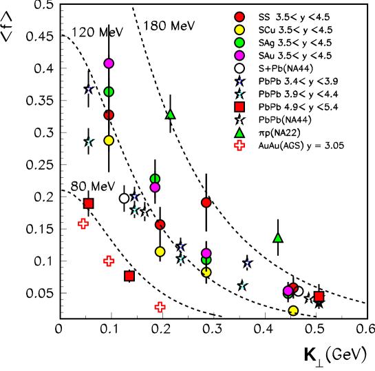
As a simple test of the thermalization assumption, one has compared [112, 52] the measured phase-space densities in Figs. 3.3 and 3.4 to that of a thermal Bose-Einstein equilibrium distribution

$$f^{\rm BE}(K_{\perp},Y)={1\over{\exp\left[M_{\perp}\cosh(Y-{\rm y}_{s})/T\right]-1}}$$ (3.73)

at pair rapidity $Y$ for a source rapidity ${\rm y}_{s}$, extracting the temperature from the measured single-particle spectra and two-particle correlations. Dynamical flow effects alter quantitative aspects of $f^{\rm BE}(\leavevmode\mathchoice{\hbox{\rm tensysevensyfivesy\boldmath{$\displaystyle K$}}}{\hbox{\rm tensysevensyfivesy\boldmath{$\textstyle K$}}}{\hbox{\rm tensysevensyfivesy\boldmath{$\scriptstyle K$}}}{\hbox{\rm tensysevensyfivesy\boldmath{$\scriptscriptstyle K$}}})$, but qualitatively the phase-space density thus calculated compares surprisingly well with the experimentally determined one, see Figs. 3.3 and 3.4.

Chapter 4 Beyond the Gaussian parametrization

The space-time variances characterizing the Cartesian HBT radius parameters (3.10)-(3.15) can be written as second derivatives of the correlator (3.5) at $\leavevmode\mathchoice{\hbox{\rm tensysevensyfivesy\boldmath{$\displaystyle q$}}}{\hbox{\rm tensysevensyfivesy\boldmath{$\textstyle q$}}}{\hbox{\rm tensysevensyfivesy\boldmath{$\scriptstyle q$}}}{\hbox{\rm tensysevensyfivesy\boldmath{$\scriptscriptstyle q$}}}=0$:

$$\langle(\tilde{x}_{i}-{\beta}_{i}\tilde{t})(\tilde{x}_{j}-{\beta}_{j}\tilde{t})\rangle\,=-\left.{\partial^{2}C(\leavevmode\mathchoice{\hbox{\rm tensysevensyfivesy\boldmath{$\displaystyle q$}}}{\hbox{\rm tensysevensyfivesy\boldmath{$\textstyle q$}}}{\hbox{\rm tensysevensyfivesy\boldmath{$\scriptstyle q$}}}{\hbox{\rm tensysevensyfivesy\boldmath{$\scriptscriptstyle q$}}},\leavevmode\mathchoice{\hbox{\rm tensysevensyfivesy\boldmath{$\displaystyle K$}}}{\hbox{\rm tensysevensyfivesy\boldmath{$\textstyle K$}}}{\hbox{\rm tensysevensyfivesy\boldmath{$\scriptstyle K$}}}{\hbox{\rm tensysevensyfivesy\boldmath{$\scriptscriptstyle K$}}})\over\partial q_{i}\,\partial q_{j}}\right|_{\leavevmode\mathchoice{\hbox{\rm tensysevensyfivesy\boldmath{$\displaystyle q$}}}{\hbox{\rm tensysevensyfivesy\boldmath{$\textstyle q$}}}{\hbox{\rm tensysevensyfivesy\boldmath{$\scriptstyle q$}}}{\hbox{\rm tensysevensyfivesy\boldmath{$\scriptscriptstyle q$}}}=0}\,.$$ (4.1)

These curvature terms coincide with the experimentally determined half widths of $C(\leavevmode\mathchoice{\hbox{\rm tensysevensyfivesy\boldmath{$\displaystyle q$}}}{\hbox{\rm tensysevensyfivesy\boldmath{$\textstyle q$}}}{\hbox{\rm tensysevensyfivesy\boldmath{$\scriptstyle q$}}}{\hbox{\rm tensysevensyfivesy\boldmath{$\scriptscriptstyle q$}}},\leavevmode\mathchoice{\hbox{\rm tensysevensyfivesy\boldmath{$\displaystyle K$}}}{\hbox{\rm tensysevensyfivesy\boldmath{$\textstyle K$}}}{\hbox{\rm tensysevensyfivesy\boldmath{$\scriptstyle K$}}}{\hbox{\rm tensysevensyfivesy\boldmath{$\scriptscriptstyle K$}}})$ only if the correlators is a Gaussian in tensysevensyfivesy$\textstyle q$. Realistic two-particle correlation functions show, however, more or less significant deviations from a Gaussian shape. The consequences are two-fold: the corresponding space-time variances do not agree exactly with the fitted radius parameters, and the Gaussian radius parameters do not contain all the information contained in $C(\leavevmode\mathchoice{\hbox{\rm tensysevensyfivesy\boldmath{$\displaystyle q$}}}{\hbox{\rm tensysevensyfivesy\boldmath{$\textstyle q$}}}{\hbox{\rm tensysevensyfivesy\boldmath{$\scriptstyle q$}}}{\hbox{\rm tensysevensyfivesy\boldmath{$\scriptscriptstyle q$}}},\leavevmode\mathchoice{\hbox{\rm tensysevensyfivesy\boldmath{$\displaystyle K$}}}{\hbox{\rm tensysevensyfivesy\boldmath{$\textstyle K$}}}{\hbox{\rm tensysevensyfivesy\boldmath{$\scriptstyle K$}}}{\hbox{\rm tensysevensyfivesy\boldmath{$\scriptscriptstyle K$}}})$. Nevertheless, qualtitatively all statements made above about mixing of spatial and temporal information in the HBT radius parameters remain valid. The reason is that the Fourier exponent $q\cdot x$ in (2.24) can be written as $\leavevmode\mathchoice{\hbox{\rm tensysevensyfivesy\boldmath{$\displaystyle q$}}}{\hbox{\rm tensysevensyfivesy\boldmath{$\textstyle q$}}}{\hbox{\rm tensysevensyfivesy\boldmath{$\scriptstyle q$}}}{\hbox{\rm tensysevensyfivesy\boldmath{$\scriptscriptstyle q$}}}\cdot\left(\leavevmode\mathchoice{\hbox{\rm tensysevensyfivesy\boldmath{$\displaystyle\beta$}}}{\hbox{\rm tensysevensyfivesy\boldmath{$\textstyle\beta$}}}{\hbox{\rm tensysevensyfivesy\boldmath{$\scriptstyle\beta$}}}{\hbox{\rm tensysevensyfivesy\boldmath{$\scriptscriptstyle\beta$}}}t\,-\leavevmode\mathchoice{\hbox{\rm tensysevensyfivesy\boldmath{$\displaystyle x$}}}{\hbox{\rm tensysevensyfivesy\boldmath{$\textstyle x$}}}{\hbox{\rm tensysevensyfivesy\boldmath{$\scriptstyle x$}}}{\hbox{\rm tensysevensyfivesy\boldmath{$\scriptscriptstyle x$}}}\right)$. Hence, the tensysevensyfivesy$\textstyle q$ dependence of the correlator tests always the same combinations $\left(\beta_{i}t\,-x_{i}\right)$ of spatial and temporal aspects of the emission function $S(x,K)$, irrespective of the shape of the two-particle correlator.

If the correlator deviates from a Gaussian shape, one can either seek a more detailed characterization of $C(\leavevmode\mathchoice{\hbox{\rm tensysevensyfivesy\boldmath{$\displaystyle q$}}}{\hbox{\rm tensysevensyfivesy\boldmath{$\textstyle q$}}}{\hbox{\rm tensysevensyfivesy\boldmath{$\scriptstyle q$}}}{\hbox{\rm tensysevensyfivesy\boldmath{$\scriptscriptstyle q$}}},\leavevmode\mathchoice{\hbox{\rm tensysevensyfivesy\boldmath{$\displaystyle K$}}}{\hbox{\rm tensysevensyfivesy\boldmath{$\textstyle K$}}}{\hbox{\rm tensysevensyfivesy\boldmath{$\scriptstyle K$}}}{\hbox{\rm tensysevensyfivesy\boldmath{$\scriptscriptstyle K$}}})$ supplementing the Gaussian radius parameters by a larger set of characteristic parameters, or one may proceed to reconstruct from the measured correlations directly information about the emission function without invoking a particular parametrization. In the following we discuss both of these strategies.

4.1 Imaging methods

Instead of determining information about the emission function $S(x,K)$, an alternative analysis strategy [37] aims at determining directly from the measured true correlator $C(\leavevmode\mathchoice{\hbox{\rm tensysevensyfivesy\boldmath{$\displaystyle q$}}}{\hbox{\rm tensysevensyfivesy\boldmath{$\textstyle q$}}}{\hbox{\rm tensysevensyfivesy\boldmath{$\scriptstyle q$}}}{\hbox{\rm tensysevensyfivesy\boldmath{$\scriptscriptstyle q$}}},\leavevmode\mathchoice{\hbox{\rm tensysevensyfivesy\boldmath{$\displaystyle K$}}}{\hbox{\rm tensysevensyfivesy\boldmath{$\textstyle K$}}}{\hbox{\rm tensysevensyfivesy\boldmath{$\scriptstyle K$}}}{\hbox{\rm tensysevensyfivesy\boldmath{$\scriptscriptstyle K$}}})-1$ the relative source function $S_{\leavevmode\mathchoice{\hbox{\rm tensysevensyfivesy\boldmath{$\displaystyle K$}}}{\hbox{\rm tensysevensyfivesy\boldmath{$\textstyle K$}}}{\hbox{\rm tensysevensyfivesy\boldmath{$\scriptstyle K$}}}{\hbox{\rm tensysevensyfivesy\boldmath{$\scriptscriptstyle K$}}}}(\leavevmode\mathchoice{\hbox{\rm tensysevensyfivesy\boldmath{$\displaystyle r$}}}{\hbox{\rm tensysevensyfivesy\boldmath{$\textstyle r$}}}{\hbox{\rm tensysevensyfivesy\boldmath{$\scriptstyle r$}}}{\hbox{\rm tensysevensyfivesy\boldmath{$\scriptscriptstyle r$}}})$ introduced in section (2.2.4):

$$C(\leavevmode\mathchoice{\hbox{\rm tensysevensyfivesy\boldmath{$\displaystyle q$}}}{\hbox{\rm tensysevensyfivesy\boldmath{$\textstyle q$}}}{\hbox{\rm tensysevensyfivesy\boldmath{$\scriptstyle q$}}}{\hbox{\rm tensysevensyfivesy\boldmath{$\scriptscriptstyle q$}}},\leavevmode\mathchoice{\hbox{\rm tensysevensyfivesy\boldmath{$\displaystyle K$}}}{\hbox{\rm tensysevensyfivesy\boldmath{$\textstyle K$}}}{\hbox{\rm tensysevensyfivesy\boldmath{$\scriptstyle K$}}}{\hbox{\rm tensysevensyfivesy\boldmath{$\scriptscriptstyle K$}}})-1=\int d^{3}r\,K(\leavevmode\mathchoice{\hbox{\rm tensysevensyfivesy\boldmath{$\displaystyle q$}}}{\hbox{\rm tensysevensyfivesy\boldmath{$\textstyle q$}}}{\hbox{\rm tensysevensyfivesy\boldmath{$\scriptstyle q$}}}{\hbox{\rm tensysevensyfivesy\boldmath{$\scriptscriptstyle q$}}},\leavevmode\mathchoice{\hbox{\rm tensysevensyfivesy\boldmath{$\displaystyle r$}}}{\hbox{\rm tensysevensyfivesy\boldmath{$\textstyle r$}}}{\hbox{\rm tensysevensyfivesy\boldmath{$\scriptstyle r$}}}{\hbox{\rm tensysevensyfivesy\boldmath{$\scriptscriptstyle r$}}})\,S_{\leavevmode\mathchoice{\hbox{\rm tensysevensyfivesy\boldmath{$\displaystyle K$}}}{\hbox{\rm tensysevensyfivesy\boldmath{$\textstyle K$}}}{\hbox{\rm tensysevensyfivesy\boldmath{$\scriptstyle K$}}}{\hbox{\rm tensysevensyfivesy\boldmath{$\scriptscriptstyle K$}}}}(\leavevmode\mathchoice{\hbox{\rm tensysevensyfivesy\boldmath{$\displaystyle r$}}}{\hbox{\rm tensysevensyfivesy\boldmath{$\textstyle r$}}}{\hbox{\rm tensysevensyfivesy\boldmath{$\scriptstyle r$}}}{\hbox{\rm tensysevensyfivesy\boldmath{$\scriptscriptstyle r$}}})\,.$$ (4.2)

For the kernel, one usually chooses $K(\leavevmode\mathchoice{\hbox{\rm tensysevensyfivesy\boldmath{$\displaystyle q$}}}{\hbox{\rm tensysevensyfivesy\boldmath{$\textstyle q$}}}{\hbox{\rm tensysevensyfivesy\boldmath{$\scriptstyle q$}}}{\hbox{\rm tensysevensyfivesy\boldmath{$\scriptscriptstyle q$}}},\leavevmode\mathchoice{\hbox{\rm tensysevensyfivesy\boldmath{$\displaystyle r$}}}{\hbox{\rm tensysevensyfivesy\boldmath{$\textstyle r$}}}{\hbox{\rm tensysevensyfivesy\boldmath{$\scriptstyle r$}}}{\hbox{\rm tensysevensyfivesy\boldmath{$\scriptscriptstyle r$}}})=|\phi_{\leavevmode\mathchoice{\hbox{\rm tensysevensyfivesy\boldmath{$\displaystyle q$}}}{\hbox{\rm tensysevensyfivesy\boldmath{$\textstyle q$}}}{\hbox{\rm tensysevensyfivesy\boldmath{$\scriptstyle q$}}}{\hbox{\rm tensysevensyfivesy\boldmath{$\scriptscriptstyle q$}}}/2}(\leavevmode\mathchoice{\hbox{\rm tensysevensyfivesy\boldmath{$\displaystyle r$}}}{\hbox{\rm tensysevensyfivesy\boldmath{$\textstyle r$}}}{\hbox{\rm tensysevensyfivesy\boldmath{$\scriptstyle r$}}}{\hbox{\rm tensysevensyfivesy\boldmath{$\scriptscriptstyle r$}}})|^{2}-1$ where $\phi_{\leavevmode\mathchoice{\hbox{\rm tensysevensyfivesy\boldmath{$\displaystyle q$}}}{\hbox{\rm tensysevensyfivesy\boldmath{$\textstyle q$}}}{\hbox{\rm tensysevensyfivesy\boldmath{$\scriptstyle q$}}}{\hbox{\rm tensysevensyfivesy\boldmath{$\scriptscriptstyle q$}}}/2}$ describes the propagation of a pair, which is created with a center of mass separation tensysevensyfivesy$\textstyle r$ and detected with relative momentum tensysevensyfivesy$\textstyle q$. $\phi_{\leavevmode\mathchoice{\hbox{\rm tensysevensyfivesy\boldmath{$\displaystyle q$}}}{\hbox{\rm tensysevensyfivesy\boldmath{$\textstyle q$}}}{\hbox{\rm tensysevensyfivesy\boldmath{$\scriptstyle q$}}}{\hbox{\rm tensysevensyfivesy\boldmath{$\scriptscriptstyle q$}}}/2}$ can include two-particle final state interactions, cf. (2.102) and (2.126); for free particle propagation, $K(\leavevmode\mathchoice{\hbox{\rm tensysevensyfivesy\boldmath{$\displaystyle q$}}}{\hbox{\rm tensysevensyfivesy\boldmath{$\textstyle q$}}}{\hbox{\rm tensysevensyfivesy\boldmath{$\scriptstyle q$}}}{\hbox{\rm tensysevensyfivesy\boldmath{$\scriptscriptstyle q$}}},\leavevmode\mathchoice{\hbox{\rm tensysevensyfivesy\boldmath{$\displaystyle r$}}}{\hbox{\rm tensysevensyfivesy\boldmath{$\textstyle r$}}}{\hbox{\rm tensysevensyfivesy\boldmath{$\scriptstyle r$}}}{\hbox{\rm tensysevensyfivesy\boldmath{$\scriptscriptstyle r$}}})=\cos(\leavevmode\mathchoice{\hbox{\rm tensysevensyfivesy\boldmath{$\displaystyle q$}}}{\hbox{\rm tensysevensyfivesy\boldmath{$\textstyle q$}}}{\hbox{\rm tensysevensyfivesy\boldmath{$\scriptstyle q$}}}{\hbox{\rm tensysevensyfivesy\boldmath{$\scriptscriptstyle q$}}}\cdot\leavevmode\mathchoice{\hbox{\rm tensysevensyfivesy\boldmath{$\displaystyle r$}}}{\hbox{\rm tensysevensyfivesy\boldmath{$\textstyle r$}}}{\hbox{\rm tensysevensyfivesy\boldmath{$\scriptstyle r$}}}{\hbox{\rm tensysevensyfivesy\boldmath{$\scriptscriptstyle r$}}})$.

Equation (4.2) can be inverted uniquely, allowing in principle for an unambiguous reconstruction of the relative source function $S_{\leavevmode\mathchoice{\hbox{\rm tensysevensyfivesy\boldmath{$\displaystyle K$}}}{\hbox{\rm tensysevensyfivesy\boldmath{$\textstyle K$}}}{\hbox{\rm tensysevensyfivesy\boldmath{$\scriptstyle K$}}}{\hbox{\rm tensysevensyfivesy\boldmath{$\scriptscriptstyle K$}}}}(\leavevmode\mathchoice{\hbox{\rm tensysevensyfivesy\boldmath{$\displaystyle r$}}}{\hbox{\rm tensysevensyfivesy\boldmath{$\textstyle r$}}}{\hbox{\rm tensysevensyfivesy\boldmath{$\scriptstyle r$}}}{\hbox{\rm tensysevensyfivesy\boldmath{$\scriptscriptstyle r$}}})$. In practice, finite measurement statistics on the correlation function and the strongly oscillating nature of the kernel $K(\leavevmode\mathchoice{\hbox{\rm tensysevensyfivesy\boldmath{$\displaystyle q$}}}{\hbox{\rm tensysevensyfivesy\boldmath{$\textstyle q$}}}{\hbox{\rm tensysevensyfivesy\boldmath{$\scriptstyle q$}}}{\hbox{\rm tensysevensyfivesy\boldmath{$\scriptscriptstyle q$}}},\leavevmode\mathchoice{\hbox{\rm tensysevensyfivesy\boldmath{$\displaystyle r$}}}{\hbox{\rm tensysevensyfivesy\boldmath{$\textstyle r$}}}{\hbox{\rm tensysevensyfivesy\boldmath{$\scriptstyle r$}}}{\hbox{\rm tensysevensyfivesy\boldmath{$\scriptscriptstyle r$}}})$ render the inversion problem non-trivial. Brown and Danielewicz [37] suggest to parametrize $S_{\leavevmode\mathchoice{\hbox{\rm tensysevensyfivesy\boldmath{$\displaystyle K$}}}{\hbox{\rm tensysevensyfivesy\boldmath{$\textstyle K$}}}{\hbox{\rm tensysevensyfivesy\boldmath{$\scriptstyle K$}}}{\hbox{\rm tensysevensyfivesy\boldmath{$\scriptscriptstyle K$}}}}(\leavevmode\mathchoice{\hbox{\rm tensysevensyfivesy\boldmath{$\displaystyle r$}}}{\hbox{\rm tensysevensyfivesy\boldmath{$\textstyle r$}}}{\hbox{\rm tensysevensyfivesy\boldmath{$\scriptstyle r$}}}{\hbox{\rm tensysevensyfivesy\boldmath{$\scriptscriptstyle r$}}})$ in terms of a finite number of basis functions $g_{j}(\leavevmode\mathchoice{\hbox{\rm tensysevensyfivesy\boldmath{$\displaystyle r$}}}{\hbox{\rm tensysevensyfivesy\boldmath{$\textstyle r$}}}{\hbox{\rm tensysevensyfivesy\boldmath{$\scriptstyle r$}}}{\hbox{\rm tensysevensyfivesy\boldmath{$\scriptscriptstyle r$}}})$,

$$S_{\leavevmode\mathchoice{\hbox{\rm tensysevensyfivesy\boldmath{$\displaystyle K$}}}{\hbox{\rm tensysevensyfivesy\boldmath{$\textstyle K$}}}{\hbox{\rm tensysevensyfivesy\boldmath{$\scriptstyle K$}}}{\hbox{\rm tensysevensyfivesy\boldmath{$\scriptscriptstyle K$}}}}(\leavevmode\mathchoice{\hbox{\rm tensysevensyfivesy\boldmath{$\displaystyle r$}}}{\hbox{\rm tensysevensyfivesy\boldmath{$\textstyle r$}}}{\hbox{\rm tensysevensyfivesy\boldmath{$\scriptstyle r$}}}{\hbox{\rm tensysevensyfivesy\boldmath{$\scriptscriptstyle r$}}})=\sum_{j=1}^{N}S_{j}(\leavevmode\mathchoice{\hbox{\rm tensysevensyfivesy\boldmath{$\displaystyle K$}}}{\hbox{\rm tensysevensyfivesy\boldmath{$\textstyle K$}}}{\hbox{\rm tensysevensyfivesy\boldmath{$\scriptstyle K$}}}{\hbox{\rm tensysevensyfivesy\boldmath{$\scriptscriptstyle K$}}})\,g_{j}(\leavevmode\mathchoice{\hbox{\rm tensysevensyfivesy\boldmath{$\displaystyle r$}}}{\hbox{\rm tensysevensyfivesy\boldmath{$\textstyle r$}}}{\hbox{\rm tensysevensyfivesy\boldmath{$\scriptstyle r$}}}{\hbox{\rm tensysevensyfivesy\boldmath{$\scriptscriptstyle r$}}})\,,$$ (4.3)

and to determine the coefficients $S_{j}(\leavevmode\mathchoice{\hbox{\rm tensysevensyfivesy\boldmath{$\displaystyle K$}}}{\hbox{\rm tensysevensyfivesy\boldmath{$\textstyle K$}}}{\hbox{\rm tensysevensyfivesy\boldmath{$\scriptstyle K$}}}{\hbox{\rm tensysevensyfivesy\boldmath{$\scriptscriptstyle K$}}})$ from the data. In applications [36, 37] some insight has been gained on how the reconstruction can be optimized by choosing suitable sets of functions $g_{j}$.

4.2 $q$-moments

Rather than obtaining the HBT radius parameters from a Gaussian fit to the measured correlation function, a quantitative analysis of $C(\leavevmode\mathchoice{\hbox{\rm tensysevensyfivesy\boldmath{$\displaystyle q$}}}{\hbox{\rm tensysevensyfivesy\boldmath{$\textstyle q$}}}{\hbox{\rm tensysevensyfivesy\boldmath{$\scriptstyle q$}}}{\hbox{\rm tensysevensyfivesy\boldmath{$\scriptscriptstyle q$}}},\leavevmode\mathchoice{\hbox{\rm tensysevensyfivesy\boldmath{$\displaystyle K$}}}{\hbox{\rm tensysevensyfivesy\boldmath{$\textstyle K$}}}{\hbox{\rm tensysevensyfivesy\boldmath{$\scriptstyle K$}}}{\hbox{\rm tensysevensyfivesy\boldmath{$\scriptscriptstyle K$}}})$ can be based on expectation values $\langle\!\langle g(\leavevmode\mathchoice{\hbox{\rm tensysevensyfivesy\boldmath{$\displaystyle q$}}}{\hbox{\rm tensysevensyfivesy\boldmath{$\textstyle q$}}}{\hbox{\rm tensysevensyfivesy\boldmath{$\scriptstyle q$}}}{\hbox{\rm tensysevensyfivesy\boldmath{$\scriptscriptstyle q$}}})\rangle\!\rangle$ of the true correlator $C(\leavevmode\mathchoice{\hbox{\rm tensysevensyfivesy\boldmath{$\displaystyle q$}}}{\hbox{\rm tensysevensyfivesy\boldmath{$\textstyle q$}}}{\hbox{\rm tensysevensyfivesy\boldmath{$\scriptstyle q$}}}{\hbox{\rm tensysevensyfivesy\boldmath{$\scriptscriptstyle q$}}},\leavevmode\mathchoice{\hbox{\rm tensysevensyfivesy\boldmath{$\displaystyle K$}}}{\hbox{\rm tensysevensyfivesy\boldmath{$\textstyle K$}}}{\hbox{\rm tensysevensyfivesy\boldmath{$\scriptstyle K$}}}{\hbox{\rm tensysevensyfivesy\boldmath{$\scriptscriptstyle K$}}})-1$ in relative momentum space [172, 173]:

$\displaystyle{\langle\!\langle q_{i}\,q_{j}\rangle\!\rangle}$ $\displaystyle=$ $\displaystyle{\int d^{3}q\,\,q_{i}\,q_{j}\,\,{[{C(\leavevmode\mathchoice{\hbox{\rm tensysevensyfivesy\boldmath{$\displaystyle q$}}}{\hbox{\rm tensysevensyfivesy\boldmath{$\textstyle q$}}}{\hbox{\rm tensysevensyfivesy\boldmath{$\scriptstyle q$}}}{\hbox{\rm tensysevensyfivesy\boldmath{$\scriptscriptstyle q$}}},\leavevmode\mathchoice{\hbox{\rm tensysevensyfivesy\boldmath{$\displaystyle K$}}}{\hbox{\rm tensysevensyfivesy\boldmath{$\textstyle K$}}}{\hbox{\rm tensysevensyfivesy\boldmath{$\scriptstyle K$}}}{\hbox{\rm tensysevensyfivesy\boldmath{$\scriptscriptstyle K$}}})-1}]}\over\int d^{3}q\,{[{C(\leavevmode\mathchoice{\hbox{\rm tensysevensyfivesy\boldmath{$\displaystyle q$}}}{\hbox{\rm tensysevensyfivesy\boldmath{$\textstyle q$}}}{\hbox{\rm tensysevensyfivesy\boldmath{$\scriptstyle q$}}}{\hbox{\rm tensysevensyfivesy\boldmath{$\scriptscriptstyle q$}}},\leavevmode\mathchoice{\hbox{\rm tensysevensyfivesy\boldmath{$\displaystyle K$}}}{\hbox{\rm tensysevensyfivesy\boldmath{$\textstyle K$}}}{\hbox{\rm tensysevensyfivesy\boldmath{$\scriptstyle K$}}}{\hbox{\rm tensysevensyfivesy\boldmath{$\scriptscriptstyle K$}}})-1}]}}={\textstyle{1\over 2}}\,{\left({R^{-1}(\leavevmode\mathchoice{\hbox{\rm tensysevensyfivesy\boldmath{$\displaystyle K$}}}{\hbox{\rm tensysevensyfivesy\boldmath{$\textstyle K$}}}{\hbox{\rm tensysevensyfivesy\boldmath{$\scriptstyle K$}}}{\hbox{\rm tensysevensyfivesy\boldmath{$\scriptscriptstyle K$}}})}\right)}_{ij},$ (4.4)
$\displaystyle R_{ij}(\leavevmode\mathchoice{\hbox{\rm tensysevensyfivesy\boldmath{$\displaystyle K$}}}{\hbox{\rm tensysevensyfivesy\boldmath{$\textstyle K$}}}{\hbox{\rm tensysevensyfivesy\boldmath{$\scriptstyle K$}}}{\hbox{\rm tensysevensyfivesy\boldmath{$\scriptscriptstyle K$}}})$ $\displaystyle=$ $\displaystyle\left(\begin{array}[]{ccc}R_{o}^{2}&R_{os}^{2}&R_{ol}^{2}\\ R_{os}^{2}&R_{s}^{2}&R_{sl}^{2}\\ R_{ol}^{2}&R_{sl}^{2}&R_{l}^{2}\end{array}\right)\,,\qquad i,j=o,s,l\,,$ (4.8)
$\displaystyle\lambda(\leavevmode\mathchoice{\hbox{\rm tensysevensyfivesy\boldmath{$\displaystyle K$}}}{\hbox{\rm tensysevensyfivesy\boldmath{$\textstyle K$}}}{\hbox{\rm tensysevensyfivesy\boldmath{$\scriptstyle K$}}}{\hbox{\rm tensysevensyfivesy\boldmath{$\scriptscriptstyle K$}}})$ $\displaystyle=$ $\displaystyle\sqrt{\det R(\leavevmode\mathchoice{\hbox{\rm tensysevensyfivesy\boldmath{$\displaystyle K$}}}{\hbox{\rm tensysevensyfivesy\boldmath{$\textstyle K$}}}{\hbox{\rm tensysevensyfivesy\boldmath{$\scriptstyle K$}}}{\hbox{\rm tensysevensyfivesy\boldmath{$\scriptscriptstyle K$}}})/\pi^{3}}\int d^{3}q\,{[{C(\leavevmode\mathchoice{\hbox{\rm tensysevensyfivesy\boldmath{$\displaystyle q$}}}{\hbox{\rm tensysevensyfivesy\boldmath{$\textstyle q$}}}{\hbox{\rm tensysevensyfivesy\boldmath{$\scriptstyle q$}}}{\hbox{\rm tensysevensyfivesy\boldmath{$\scriptscriptstyle q$}}},\leavevmode\mathchoice{\hbox{\rm tensysevensyfivesy\boldmath{$\displaystyle K$}}}{\hbox{\rm tensysevensyfivesy\boldmath{$\textstyle K$}}}{\hbox{\rm tensysevensyfivesy\boldmath{$\scriptstyle K$}}}{\hbox{\rm tensysevensyfivesy\boldmath{$\scriptscriptstyle K$}}})-1}]}\,.$ (4.9)

Similar expressions exist for the YKP parameters [172]. For a Gaussian correlator, the intercept parameter $\lambda$ and the HBT radius parameters $R_{ij}^{2}$ obtained via these $q$-moments coincide with the values extracted from a Gaussian fit. For non-Gaussian correlators the HBT radius parameters and the intercept can be defined via (4.4)-(4.9).

Deviations of the correlator from a Gaussian shape are then quantified by higher order $q$-moments, which in turn can be obtained as derivatives of the generating function $Z(\leavevmode\mathchoice{\hbox{\rm tensysevensyfivesy\boldmath{$\displaystyle y$}}}{\hbox{\rm tensysevensyfivesy\boldmath{$\textstyle y$}}}{\hbox{\rm tensysevensyfivesy\boldmath{$\scriptstyle y$}}}{\hbox{\rm tensysevensyfivesy\boldmath{$\scriptscriptstyle y$}}},\leavevmode\mathchoice{\hbox{\rm tensysevensyfivesy\boldmath{$\displaystyle K$}}}{\hbox{\rm tensysevensyfivesy\boldmath{$\textstyle K$}}}{\hbox{\rm tensysevensyfivesy\boldmath{$\scriptstyle K$}}}{\hbox{\rm tensysevensyfivesy\boldmath{$\scriptscriptstyle K$}}})$,

$\displaystyle Z(\leavevmode\mathchoice{\hbox{\rm tensysevensyfivesy\boldmath{$\displaystyle y$}}}{\hbox{\rm tensysevensyfivesy\boldmath{$\textstyle y$}}}{\hbox{\rm tensysevensyfivesy\boldmath{$\scriptstyle y$}}}{\hbox{\rm tensysevensyfivesy\boldmath{$\scriptscriptstyle y$}}},\leavevmode\mathchoice{\hbox{\rm tensysevensyfivesy\boldmath{$\displaystyle K$}}}{\hbox{\rm tensysevensyfivesy\boldmath{$\textstyle K$}}}{\hbox{\rm tensysevensyfivesy\boldmath{$\scriptstyle K$}}}{\hbox{\rm tensysevensyfivesy\boldmath{$\scriptscriptstyle K$}}})$ $\displaystyle=$ $\displaystyle\int d^{3}q\,e^{i\leavevmode\mathchoice{\hbox{\rm tensysevensyfivesy\boldmath{$\displaystyle q$}}}{\hbox{\rm tensysevensyfivesy\boldmath{$\textstyle q$}}}{\hbox{\rm tensysevensyfivesy\boldmath{$\scriptstyle q$}}}{\hbox{\rm tensysevensyfivesy\boldmath{$\scriptscriptstyle q$}}}\cdot\leavevmode\mathchoice{\hbox{\rm tensysevensyfivesy\boldmath{$\displaystyle y$}}}{\hbox{\rm tensysevensyfivesy\boldmath{$\textstyle y$}}}{\hbox{\rm tensysevensyfivesy\boldmath{$\scriptstyle y$}}}{\hbox{\rm tensysevensyfivesy\boldmath{$\scriptscriptstyle y$}}}}\,{[{C(\leavevmode\mathchoice{\hbox{\rm tensysevensyfivesy\boldmath{$\displaystyle q$}}}{\hbox{\rm tensysevensyfivesy\boldmath{$\textstyle q$}}}{\hbox{\rm tensysevensyfivesy\boldmath{$\scriptstyle q$}}}{\hbox{\rm tensysevensyfivesy\boldmath{$\scriptscriptstyle q$}}},\leavevmode\mathchoice{\hbox{\rm tensysevensyfivesy\boldmath{$\displaystyle K$}}}{\hbox{\rm tensysevensyfivesy\boldmath{$\textstyle K$}}}{\hbox{\rm tensysevensyfivesy\boldmath{$\scriptstyle K$}}}{\hbox{\rm tensysevensyfivesy\boldmath{$\scriptscriptstyle K$}}})-1}]}\,,$ (4.10)
$\displaystyle{\langle\!\langle{q_{i_{1}}\cdots q_{i_{n}}}\rangle\!\rangle}$ $\displaystyle=$ $\displaystyle{(-i\partial)^{n}\over\partial y_{i_{1}}\cdots\partial y_{i_{n}}}\ln Z(\leavevmode\mathchoice{\hbox{\rm tensysevensyfivesy\boldmath{$\displaystyle y$}}}{\hbox{\rm tensysevensyfivesy\boldmath{$\textstyle y$}}}{\hbox{\rm tensysevensyfivesy\boldmath{$\scriptstyle y$}}}{\hbox{\rm tensysevensyfivesy\boldmath{$\scriptscriptstyle y$}}},\leavevmode\mathchoice{\hbox{\rm tensysevensyfivesy\boldmath{$\displaystyle K$}}}{\hbox{\rm tensysevensyfivesy\boldmath{$\textstyle K$}}}{\hbox{\rm tensysevensyfivesy\boldmath{$\scriptstyle K$}}}{\hbox{\rm tensysevensyfivesy\boldmath{$\scriptscriptstyle K$}}})\bigg{|}_{\leavevmode\mathchoice{\hbox{\rm tensysevensyfivesy\boldmath{$\displaystyle y$}}}{\hbox{\rm tensysevensyfivesy\boldmath{$\textstyle y$}}}{\hbox{\rm tensysevensyfivesy\boldmath{$\scriptstyle y$}}}{\hbox{\rm tensysevensyfivesy\boldmath{$\scriptscriptstyle y$}}}=0}\,.$ (4.11)

It is easy to see that $Z(\leavevmode\mathchoice{\hbox{\rm tensysevensyfivesy\boldmath{$\displaystyle y$}}}{\hbox{\rm tensysevensyfivesy\boldmath{$\textstyle y$}}}{\hbox{\rm tensysevensyfivesy\boldmath{$\scriptstyle y$}}}{\hbox{\rm tensysevensyfivesy\boldmath{$\scriptscriptstyle y$}}},\leavevmode\mathchoice{\hbox{\rm tensysevensyfivesy\boldmath{$\displaystyle K$}}}{\hbox{\rm tensysevensyfivesy\boldmath{$\textstyle K$}}}{\hbox{\rm tensysevensyfivesy\boldmath{$\scriptstyle K$}}}{\hbox{\rm tensysevensyfivesy\boldmath{$\scriptscriptstyle K$}}})$ coincides with the relative source function (2.31)

$$Z(\leavevmode\mathchoice{\hbox{\rm tensysevensyfivesy\boldmath{$\displaystyle y$}}}{\hbox{\rm tensysevensyfivesy\boldmath{$\textstyle y$}}}{\hbox{\rm tensysevensyfivesy\boldmath{$\scriptstyle y$}}}{\hbox{\rm tensysevensyfivesy\boldmath{$\scriptscriptstyle y$}}},\leavevmode\mathchoice{\hbox{\rm tensysevensyfivesy\boldmath{$\displaystyle K$}}}{\hbox{\rm tensysevensyfivesy\boldmath{$\textstyle K$}}}{\hbox{\rm tensysevensyfivesy\boldmath{$\scriptstyle K$}}}{\hbox{\rm tensysevensyfivesy\boldmath{$\scriptscriptstyle K$}}})=S_{\leavevmode\mathchoice{\hbox{\rm tensysevensyfivesy\boldmath{$\displaystyle K$}}}{\hbox{\rm tensysevensyfivesy\boldmath{$\textstyle K$}}}{\hbox{\rm tensysevensyfivesy\boldmath{$\scriptstyle K$}}}{\hbox{\rm tensysevensyfivesy\boldmath{$\scriptscriptstyle K$}}}}(\leavevmode\mathchoice{\hbox{\rm tensysevensyfivesy\boldmath{$\displaystyle y$}}}{\hbox{\rm tensysevensyfivesy\boldmath{$\textstyle y$}}}{\hbox{\rm tensysevensyfivesy\boldmath{$\scriptstyle y$}}}{\hbox{\rm tensysevensyfivesy\boldmath{$\scriptscriptstyle y$}}})\,.$$ (4.12)

So far, only the uni-directional version of these expressions has been used in theoretical and experimental investigations [98]: Restricting the correlator along one of the three Cartesian axes, $\tilde{C}(\leavevmode\mathchoice{\hbox{\rm tensysevensyfivesy\boldmath{$\displaystyle K$}}}{\hbox{\rm tensysevensyfivesy\boldmath{$\textstyle K$}}}{\hbox{\rm tensysevensyfivesy\boldmath{$\scriptstyle K$}}}{\hbox{\rm tensysevensyfivesy\boldmath{$\scriptscriptstyle K$}}},q_{i})\equiv C(\leavevmode\mathchoice{\hbox{\rm tensysevensyfivesy\boldmath{$\displaystyle K$}}}{\hbox{\rm tensysevensyfivesy\boldmath{$\textstyle K$}}}{\hbox{\rm tensysevensyfivesy\boldmath{$\scriptstyle K$}}}{\hbox{\rm tensysevensyfivesy\boldmath{$\scriptscriptstyle K$}}},q_{i},q_{j\neq i}{=}0)$, the corresponding HBT radius parameter and intercept are defined via the relations (we use the same notation as for the three-dimensional $q$-moments)

$\displaystyle R_{i}^{2}(\leavevmode\mathchoice{\hbox{\rm tensysevensyfivesy\boldmath{$\displaystyle K$}}}{\hbox{\rm tensysevensyfivesy\boldmath{$\textstyle K$}}}{\hbox{\rm tensysevensyfivesy\boldmath{$\scriptstyle K$}}}{\hbox{\rm tensysevensyfivesy\boldmath{$\scriptscriptstyle K$}}})$ $\displaystyle=$ $\displaystyle{1\over 2\,\langle\!\langle q_{i}^{2}\rangle\!\rangle}\,,\qquad i=o,s,l,$ (4.13)
$\displaystyle\langle\!\langle q_{i}^{2}\rangle\!\rangle(\leavevmode\mathchoice{\hbox{\rm tensysevensyfivesy\boldmath{$\displaystyle K$}}}{\hbox{\rm tensysevensyfivesy\boldmath{$\textstyle K$}}}{\hbox{\rm tensysevensyfivesy\boldmath{$\scriptstyle K$}}}{\hbox{\rm tensysevensyfivesy\boldmath{$\scriptscriptstyle K$}}})$ $\displaystyle=$ $\displaystyle{\int dq_{i}\,q_{i}^{2}\,[\tilde{C}(\leavevmode\mathchoice{\hbox{\rm tensysevensyfivesy\boldmath{$\displaystyle K$}}}{\hbox{\rm tensysevensyfivesy\boldmath{$\textstyle K$}}}{\hbox{\rm tensysevensyfivesy\boldmath{$\scriptstyle K$}}}{\hbox{\rm tensysevensyfivesy\boldmath{$\scriptscriptstyle K$}}},q_{i})-1]\over\int dq_{i}\,[\tilde{C}(\leavevmode\mathchoice{\hbox{\rm tensysevensyfivesy\boldmath{$\displaystyle K$}}}{\hbox{\rm tensysevensyfivesy\boldmath{$\textstyle K$}}}{\hbox{\rm tensysevensyfivesy\boldmath{$\scriptstyle K$}}}{\hbox{\rm tensysevensyfivesy\boldmath{$\scriptscriptstyle K$}}},q_{i})-1]}\,,$ (4.14)
$\displaystyle\lambda_{i}(\leavevmode\mathchoice{\hbox{\rm tensysevensyfivesy\boldmath{$\displaystyle K$}}}{\hbox{\rm tensysevensyfivesy\boldmath{$\textstyle K$}}}{\hbox{\rm tensysevensyfivesy\boldmath{$\scriptstyle K$}}}{\hbox{\rm tensysevensyfivesy\boldmath{$\scriptscriptstyle K$}}})$ $\displaystyle=$ $\displaystyle(R_{i}(\leavevmode\mathchoice{\hbox{\rm tensysevensyfivesy\boldmath{$\displaystyle K$}}}{\hbox{\rm tensysevensyfivesy\boldmath{$\textstyle K$}}}{\hbox{\rm tensysevensyfivesy\boldmath{$\scriptstyle K$}}}{\hbox{\rm tensysevensyfivesy\boldmath{$\scriptscriptstyle K$}}})/\sqrt{\pi})\int dq_{i}\,[\tilde{C}(\leavevmode\mathchoice{\hbox{\rm tensysevensyfivesy\boldmath{$\displaystyle K$}}}{\hbox{\rm tensysevensyfivesy\boldmath{$\textstyle K$}}}{\hbox{\rm tensysevensyfivesy\boldmath{$\scriptstyle K$}}}{\hbox{\rm tensysevensyfivesy\boldmath{$\scriptscriptstyle K$}}},q_{i})-1]\,.$ (4.15)

In the case of deviations of $C(\leavevmode\mathchoice{\hbox{\rm tensysevensyfivesy\boldmath{$\displaystyle q$}}}{\hbox{\rm tensysevensyfivesy\boldmath{$\textstyle q$}}}{\hbox{\rm tensysevensyfivesy\boldmath{$\scriptstyle q$}}}{\hbox{\rm tensysevensyfivesy\boldmath{$\scriptscriptstyle q$}}},\leavevmode\mathchoice{\hbox{\rm tensysevensyfivesy\boldmath{$\displaystyle K$}}}{\hbox{\rm tensysevensyfivesy\boldmath{$\textstyle K$}}}{\hbox{\rm tensysevensyfivesy\boldmath{$\scriptstyle K$}}}{\hbox{\rm tensysevensyfivesy\boldmath{$\scriptscriptstyle K$}}})$ from a Gaussian form, the intercepts $\lambda_{i}$ from uni-directional fits can differ in the different directions. A quantitative measure for the leading deviation of $C(\leavevmode\mathchoice{\hbox{\rm tensysevensyfivesy\boldmath{$\displaystyle q$}}}{\hbox{\rm tensysevensyfivesy\boldmath{$\textstyle q$}}}{\hbox{\rm tensysevensyfivesy\boldmath{$\scriptstyle q$}}}{\hbox{\rm tensysevensyfivesy\boldmath{$\scriptscriptstyle q$}}},\leavevmode\mathchoice{\hbox{\rm tensysevensyfivesy\boldmath{$\displaystyle K$}}}{\hbox{\rm tensysevensyfivesy\boldmath{$\textstyle K$}}}{\hbox{\rm tensysevensyfivesy\boldmath{$\scriptstyle K$}}}{\hbox{\rm tensysevensyfivesy\boldmath{$\scriptscriptstyle K$}}})$ from a Gaussian shape is provided by the properly normalized fourth order moments, the kurtoses [172, 173]

$$\Delta_{i}(\leavevmode\mathchoice{\hbox{\rm tensysevensyfivesy\boldmath{$\displaystyle K$}}}{\hbox{\rm tensysevensyfivesy\boldmath{$\textstyle K$}}}{\hbox{\rm tensysevensyfivesy\boldmath{$\scriptstyle K$}}}{\hbox{\rm tensysevensyfivesy\boldmath{$\scriptscriptstyle K$}}})={\langle\!\langle q_{i}^{4}\rangle\!\rangle(\leavevmode\mathchoice{\hbox{\rm tensysevensyfivesy\boldmath{$\displaystyle K$}}}{\hbox{\rm tensysevensyfivesy\boldmath{$\textstyle K$}}}{\hbox{\rm tensysevensyfivesy\boldmath{$\scriptstyle K$}}}{\hbox{\rm tensysevensyfivesy\boldmath{$\scriptscriptstyle K$}}})\over 3\,\langle\!\langle q_{i}^{2}\rangle\!\rangle^{2}(\leavevmode\mathchoice{\hbox{\rm tensysevensyfivesy\boldmath{$\displaystyle K$}}}{\hbox{\rm tensysevensyfivesy\boldmath{$\textstyle K$}}}{\hbox{\rm tensysevensyfivesy\boldmath{$\scriptstyle K$}}}{\hbox{\rm tensysevensyfivesy\boldmath{$\scriptscriptstyle K$}}})}-1\,.$$ (4.16)

The uni-directional kurtosis $\Delta_{i}(\leavevmode\mathchoice{\hbox{\rm tensysevensyfivesy\boldmath{$\displaystyle K$}}}{\hbox{\rm tensysevensyfivesy\boldmath{$\textstyle K$}}}{\hbox{\rm tensysevensyfivesy\boldmath{$\scriptstyle K$}}}{\hbox{\rm tensysevensyfivesy\boldmath{$\scriptscriptstyle K$}}})$ vanishes if the correlator at pair momentum tensysevensyfivesy$\textstyle K$ is of Gaussian shape in the $q_{i}$-direction. The applications of $q$-moments to experimental data is limited by statistics: for higher order $q$-moments the main contribution to the moment integral comes from larger relative momenta, while most experimental information is concentrated at small tensysevensyfivesy$\textstyle q$.

4.3 Three-particle correlations

The complete set of $q$-moments (4.11) provides a full characterization of the shape of the two-particle correlator. Alternatively, a complete characterization of this shape could be obtained in a Taylor expansion of $C(\leavevmode\mathchoice{\hbox{\rm tensysevensyfivesy\boldmath{$\displaystyle q$}}}{\hbox{\rm tensysevensyfivesy\boldmath{$\textstyle q$}}}{\hbox{\rm tensysevensyfivesy\boldmath{$\scriptstyle q$}}}{\hbox{\rm tensysevensyfivesy\boldmath{$\scriptscriptstyle q$}}},\leavevmode\mathchoice{\hbox{\rm tensysevensyfivesy\boldmath{$\displaystyle K$}}}{\hbox{\rm tensysevensyfivesy\boldmath{$\textstyle K$}}}{\hbox{\rm tensysevensyfivesy\boldmath{$\scriptstyle K$}}}{\hbox{\rm tensysevensyfivesy\boldmath{$\scriptscriptstyle K$}}})$ around $\leavevmode\mathchoice{\hbox{\rm tensysevensyfivesy\boldmath{$\displaystyle q$}}}{\hbox{\rm tensysevensyfivesy\boldmath{$\textstyle q$}}}{\hbox{\rm tensysevensyfivesy\boldmath{$\scriptstyle q$}}}{\hbox{\rm tensysevensyfivesy\boldmath{$\scriptscriptstyle q$}}}=0$. Extending equation (4.1) to arbitrary orders, the corresponding Taylor coefficients read

$$\langle(\tilde{x}_{i_{1}}-{\beta}_{i_{1}}\tilde{t})\,(\tilde{x}_{i_{2}}-{\beta}_{i_{2}}\tilde{t})\cdots(\tilde{x}_{i_{n}}-{\beta}_{i_{n}}\tilde{t})\rangle=\left.{i^{n}\,\partial^{n}C(\leavevmode\mathchoice{\hbox{\rm tensysevensyfivesy\boldmath{$\displaystyle q$}}}{\hbox{\rm tensysevensyfivesy\boldmath{$\textstyle q$}}}{\hbox{\rm tensysevensyfivesy\boldmath{$\scriptstyle q$}}}{\hbox{\rm tensysevensyfivesy\boldmath{$\scriptscriptstyle q$}}},\leavevmode\mathchoice{\hbox{\rm tensysevensyfivesy\boldmath{$\displaystyle K$}}}{\hbox{\rm tensysevensyfivesy\boldmath{$\textstyle K$}}}{\hbox{\rm tensysevensyfivesy\boldmath{$\scriptstyle K$}}}{\hbox{\rm tensysevensyfivesy\boldmath{$\scriptscriptstyle K$}}})\over\partial q_{i_{1}}\,\partial q_{i_{2}}\cdots\partial q_{i_{n}}}\right|_{\leavevmode\mathchoice{\hbox{\rm tensysevensyfivesy\boldmath{$\displaystyle q$}}}{\hbox{\rm tensysevensyfivesy\boldmath{$\textstyle q$}}}{\hbox{\rm tensysevensyfivesy\boldmath{$\scriptstyle q$}}}{\hbox{\rm tensysevensyfivesy\boldmath{$\scriptscriptstyle q$}}}=0}\,.$$ (4.17)

However, due to finite momentum resolution, no detailed information about the curvature of $C(\leavevmode\mathchoice{\hbox{\rm tensysevensyfivesy\boldmath{$\displaystyle q$}}}{\hbox{\rm tensysevensyfivesy\boldmath{$\textstyle q$}}}{\hbox{\rm tensysevensyfivesy\boldmath{$\scriptstyle q$}}}{\hbox{\rm tensysevensyfivesy\boldmath{$\scriptscriptstyle q$}}},\leavevmode\mathchoice{\hbox{\rm tensysevensyfivesy\boldmath{$\displaystyle K$}}}{\hbox{\rm tensysevensyfivesy\boldmath{$\textstyle K$}}}{\hbox{\rm tensysevensyfivesy\boldmath{$\scriptstyle K$}}}{\hbox{\rm tensysevensyfivesy\boldmath{$\scriptscriptstyle K$}}})$ at $\leavevmode\mathchoice{\hbox{\rm tensysevensyfivesy\boldmath{$\displaystyle q$}}}{\hbox{\rm tensysevensyfivesy\boldmath{$\textstyle q$}}}{\hbox{\rm tensysevensyfivesy\boldmath{$\scriptstyle q$}}}{\hbox{\rm tensysevensyfivesy\boldmath{$\scriptscriptstyle q$}}}=0$ is available from the data, and (4.17) cannot be applied in practice. It illustrates, however, clearly that the two-particle correlator $C(\leavevmode\mathchoice{\hbox{\rm tensysevensyfivesy\boldmath{$\displaystyle q$}}}{\hbox{\rm tensysevensyfivesy\boldmath{$\textstyle q$}}}{\hbox{\rm tensysevensyfivesy\boldmath{$\scriptstyle q$}}}{\hbox{\rm tensysevensyfivesy\boldmath{$\scriptscriptstyle q$}}},\leavevmode\mathchoice{\hbox{\rm tensysevensyfivesy\boldmath{$\displaystyle K$}}}{\hbox{\rm tensysevensyfivesy\boldmath{$\textstyle K$}}}{\hbox{\rm tensysevensyfivesy\boldmath{$\scriptstyle K$}}}{\hbox{\rm tensysevensyfivesy\boldmath{$\scriptscriptstyle K$}}})$ contains no information about odd space-time variances: due to the reflection symmetry $C(\leavevmode\mathchoice{\hbox{\rm tensysevensyfivesy\boldmath{$\displaystyle q$}}}{\hbox{\rm tensysevensyfivesy\boldmath{$\textstyle q$}}}{\hbox{\rm tensysevensyfivesy\boldmath{$\scriptstyle q$}}}{\hbox{\rm tensysevensyfivesy\boldmath{$\scriptscriptstyle q$}}},\leavevmode\mathchoice{\hbox{\rm tensysevensyfivesy\boldmath{$\displaystyle K$}}}{\hbox{\rm tensysevensyfivesy\boldmath{$\textstyle K$}}}{\hbox{\rm tensysevensyfivesy\boldmath{$\scriptstyle K$}}}{\hbox{\rm tensysevensyfivesy\boldmath{$\scriptscriptstyle K$}}})\leftrightarrow C(\leavevmode\mathchoice{\hbox{\rm tensysevensyfivesy\boldmath{$\displaystyle K$}}}{\hbox{\rm tensysevensyfivesy\boldmath{$\textstyle K$}}}{\hbox{\rm tensysevensyfivesy\boldmath{$\scriptstyle K$}}}{\hbox{\rm tensysevensyfivesy\boldmath{$\scriptscriptstyle K$}}},-\leavevmode\mathchoice{\hbox{\rm tensysevensyfivesy\boldmath{$\displaystyle q$}}}{\hbox{\rm tensysevensyfivesy\boldmath{$\textstyle q$}}}{\hbox{\rm tensysevensyfivesy\boldmath{$\scriptstyle q$}}}{\hbox{\rm tensysevensyfivesy\boldmath{$\scriptscriptstyle q$}}})$, all odd space-time variances in (4.17) vanish.

The true two-particle correlator $R_{2}\equiv C-1$ depends only on the modulus $\rho_{ij}$ of the Fourier transformed emission function but not on its phase $\phi_{ij}$:

$\displaystyle R_{2}(i,j)$ $\displaystyle=$ $\displaystyle C(\leavevmode\mathchoice{\hbox{\rm tensysevensyfivesy\boldmath{$\displaystyle p$}}}{\hbox{\rm tensysevensyfivesy\boldmath{$\textstyle p$}}}{\hbox{\rm tensysevensyfivesy\boldmath{$\scriptstyle p$}}}{\hbox{\rm tensysevensyfivesy\boldmath{$\scriptscriptstyle p$}}}_{i},\leavevmode\mathchoice{\hbox{\rm tensysevensyfivesy\boldmath{$\displaystyle p$}}}{\hbox{\rm tensysevensyfivesy\boldmath{$\textstyle p$}}}{\hbox{\rm tensysevensyfivesy\boldmath{$\scriptstyle p$}}}{\hbox{\rm tensysevensyfivesy\boldmath{$\scriptscriptstyle p$}}}_{j})-1={\rho_{ij}^{2}\over\rho_{ii}\,\rho_{jj}}\,,$ (4.18)
$\displaystyle\rho_{ij}\,e^{i\phi_{ij}}$ $\displaystyle=$ $\displaystyle\int d^{4}x\,S\left(x,\textstyle{1\over 2}(p_{i}+p_{j})\right)\,e^{i(p_{i}-p_{j})\cdot x}\,.$ (4.19)

Only the phase $\phi_{ij}$ contains information about odd space-time variances [80]:

$$\phi_{ij}=q_{ij}\langle x\rangle_{ij}-\textstyle{1\over 6}\langle(q_{ij}\cdot\tilde{x}_{ij})^{3}\rangle_{ij}+O(q_{ij}^{5})\,.$$ (4.20)

Here $K_{ij}$, $q_{ij}$ denote the average and relative pair momentum for two particles with on-shell momenta $p_{i}$ and $p_{j}$, respectively, and the space-time variances $\langle\,..\,\rangle_{ij}$ are calculated with respect to the emission function $S(x,K_{ij})$. Three-particle correlations give access to this phase as can be seen from [80]

$\displaystyle r_{3}(\leavevmode\mathchoice{\hbox{\rm tensysevensyfivesy\boldmath{$\displaystyle p$}}}{\hbox{\rm tensysevensyfivesy\boldmath{$\textstyle p$}}}{\hbox{\rm tensysevensyfivesy\boldmath{$\scriptstyle p$}}}{\hbox{\rm tensysevensyfivesy\boldmath{$\scriptscriptstyle p$}}}_{1},\leavevmode\mathchoice{\hbox{\rm tensysevensyfivesy\boldmath{$\displaystyle p$}}}{\hbox{\rm tensysevensyfivesy\boldmath{$\textstyle p$}}}{\hbox{\rm tensysevensyfivesy\boldmath{$\scriptstyle p$}}}{\hbox{\rm tensysevensyfivesy\boldmath{$\scriptscriptstyle p$}}}_{2},\leavevmode\mathchoice{\hbox{\rm tensysevensyfivesy\boldmath{$\displaystyle p$}}}{\hbox{\rm tensysevensyfivesy\boldmath{$\textstyle p$}}}{\hbox{\rm tensysevensyfivesy\boldmath{$\scriptstyle p$}}}{\hbox{\rm tensysevensyfivesy\boldmath{$\scriptscriptstyle p$}}}_{3})$ $\displaystyle=$ $\displaystyle{R_{3}(\leavevmode\mathchoice{\hbox{\rm tensysevensyfivesy\boldmath{$\displaystyle p$}}}{\hbox{\rm tensysevensyfivesy\boldmath{$\textstyle p$}}}{\hbox{\rm tensysevensyfivesy\boldmath{$\scriptstyle p$}}}{\hbox{\rm tensysevensyfivesy\boldmath{$\scriptscriptstyle p$}}}_{1},\leavevmode\mathchoice{\hbox{\rm tensysevensyfivesy\boldmath{$\displaystyle p$}}}{\hbox{\rm tensysevensyfivesy\boldmath{$\textstyle p$}}}{\hbox{\rm tensysevensyfivesy\boldmath{$\scriptstyle p$}}}{\hbox{\rm tensysevensyfivesy\boldmath{$\scriptscriptstyle p$}}}_{2},\leavevmode\mathchoice{\hbox{\rm tensysevensyfivesy\boldmath{$\displaystyle p$}}}{\hbox{\rm tensysevensyfivesy\boldmath{$\textstyle p$}}}{\hbox{\rm tensysevensyfivesy\boldmath{$\scriptstyle p$}}}{\hbox{\rm tensysevensyfivesy\boldmath{$\scriptscriptstyle p$}}}_{3})\over\sqrt{R_{2}(1,2)\,R_{2}(2,3)\,R_{2}(3,1)}}$ (4.21)
$\displaystyle=$ $\displaystyle 2\cos\left(\phi_{12}+\phi_{23}+\phi_{31}\right)\,,$
$\displaystyle R_{3}(\leavevmode\mathchoice{\hbox{\rm tensysevensyfivesy\boldmath{$\displaystyle p$}}}{\hbox{\rm tensysevensyfivesy\boldmath{$\textstyle p$}}}{\hbox{\rm tensysevensyfivesy\boldmath{$\scriptstyle p$}}}{\hbox{\rm tensysevensyfivesy\boldmath{$\scriptscriptstyle p$}}}_{1},\leavevmode\mathchoice{\hbox{\rm tensysevensyfivesy\boldmath{$\displaystyle p$}}}{\hbox{\rm tensysevensyfivesy\boldmath{$\textstyle p$}}}{\hbox{\rm tensysevensyfivesy\boldmath{$\scriptstyle p$}}}{\hbox{\rm tensysevensyfivesy\boldmath{$\scriptscriptstyle p$}}}_{2},\leavevmode\mathchoice{\hbox{\rm tensysevensyfivesy\boldmath{$\displaystyle p$}}}{\hbox{\rm tensysevensyfivesy\boldmath{$\textstyle p$}}}{\hbox{\rm tensysevensyfivesy\boldmath{$\scriptstyle p$}}}{\hbox{\rm tensysevensyfivesy\boldmath{$\scriptscriptstyle p$}}}_{3})$ $\displaystyle=$ $\displaystyle C_{3}(\leavevmode\mathchoice{\hbox{\rm tensysevensyfivesy\boldmath{$\displaystyle p$}}}{\hbox{\rm tensysevensyfivesy\boldmath{$\textstyle p$}}}{\hbox{\rm tensysevensyfivesy\boldmath{$\scriptstyle p$}}}{\hbox{\rm tensysevensyfivesy\boldmath{$\scriptscriptstyle p$}}}_{1},\leavevmode\mathchoice{\hbox{\rm tensysevensyfivesy\boldmath{$\displaystyle p$}}}{\hbox{\rm tensysevensyfivesy\boldmath{$\textstyle p$}}}{\hbox{\rm tensysevensyfivesy\boldmath{$\scriptstyle p$}}}{\hbox{\rm tensysevensyfivesy\boldmath{$\scriptscriptstyle p$}}}_{2},\leavevmode\mathchoice{\hbox{\rm tensysevensyfivesy\boldmath{$\displaystyle p$}}}{\hbox{\rm tensysevensyfivesy\boldmath{$\textstyle p$}}}{\hbox{\rm tensysevensyfivesy\boldmath{$\scriptstyle p$}}}{\hbox{\rm tensysevensyfivesy\boldmath{$\scriptscriptstyle p$}}}_{3})-R_{2}(1,2)$ (4.22)
$\displaystyle-R_{2}(2,3)-R_{2}(3,1)-1\,.$

Here $R_{3}$ ($r_{3}$) is the true (normalized) three-particle correlation function. To investigate the space-time information contained in the phase combination on the r.h.s. of (4.21) in more detail one can expand the emission function $S(x,K_{ij})$ in (4.19) around the average momentum of the particle triplet:

$\displaystyle\bar{K}$ $\displaystyle=$ $\displaystyle\textstyle{1\over 3}(p_{1}+p_{2}+p_{3})=\textstyle{1\over 3}(K_{12}+K_{23}+K_{31})\,,$ (4.23)
$\displaystyle K_{ij}$ $\displaystyle=$ $\displaystyle\bar{K}+\textstyle{1\over 6}(q_{ij}+q_{jk})\,,\qquad i\not=j\not=k\,.$ (4.24)

Using $q_{12}+q_{23}+q_{31}=0$ one finds [80, 86]

$\displaystyle\Phi$ $\displaystyle=$ $\displaystyle\phi_{12}+\phi_{23}+\phi_{31}$ (4.25)
$\displaystyle=$ $\displaystyle{1\over 2}\,q_{12}^{\mu}\,q_{23}^{\nu}\left[{{\partial\langle x_{\mu}\rangle_{3}}\over\partial\bar{K}^{\nu}}-{{\partial\langle x_{\nu}\rangle_{3}}\over\partial\bar{K}^{\mu}}\right]$
$\displaystyle-{1\over 24}\,[q_{12}^{\mu}\,q_{12}^{\nu}\,q_{23}^{\lambda}+q_{23}^{\mu}\,q_{23}^{\nu}\,q_{12}^{\lambda}]\left[{{\partial^{2}\langle x_{\mu}\rangle_{3}}\over\partial\bar{K}^{\nu}\partial\bar{K}^{\lambda}}+{{\partial^{2}\langle x_{\nu}\rangle_{3}}\over\partial\bar{K}^{\lambda}\partial\bar{K}^{\mu}}+{{\partial^{2}\langle x_{\lambda}\rangle_{3}}\over\partial\bar{K}^{\mu}\partial\bar{K}^{\nu}}\right]$
$\displaystyle-{1\over 2}q_{12}^{\mu}\,q_{23}^{\nu}\,(q_{12}+q_{23})^{\lambda}\,\langle\tilde{x}_{\mu}\tilde{x}_{\nu}\tilde{x}_{\lambda}\rangle_{3}+O(q^{4})\,.$

Here the averages $\langle\,\dots\,\rangle_{3}$ have been calculated with the emission function $S(x,\bar{K})$ taken at the momentum $\bar{K}$ of the particle triplet.

The measurable phase $\Phi$ depends on the odd space-time variances $\langle\tilde{x}^{3}\rangle$, etc., and on derivatives of the point of highest emissivity $\langle x\rangle_{3}$ with respect to $\bar{K}$. These reflect the asymmetries of the source around its center. In the Gaussian approximation (3.1) they vanish. These considerations show that the true three-particle correlator contains additional information which is not accessible via two-particle correlations.

In practice, however, it is very difficult to extract this information. The leading contribution to $\Phi$ is of second order in the relative momenta $q_{ij}$, and in many reasonable models it even vanishes [86]. Therefore new information typically enters $r_{3}(\leavevmode\mathchoice{\hbox{\rm tensysevensyfivesy\boldmath{$\displaystyle p$}}}{\hbox{\rm tensysevensyfivesy\boldmath{$\textstyle p$}}}{\hbox{\rm tensysevensyfivesy\boldmath{$\scriptstyle p$}}}{\hbox{\rm tensysevensyfivesy\boldmath{$\scriptscriptstyle p$}}}_{1},\leavevmode\mathchoice{\hbox{\rm tensysevensyfivesy\boldmath{$\displaystyle p$}}}{\hbox{\rm tensysevensyfivesy\boldmath{$\textstyle p$}}}{\hbox{\rm tensysevensyfivesy\boldmath{$\scriptstyle p$}}}{\hbox{\rm tensysevensyfivesy\boldmath{$\scriptscriptstyle p$}}}_{2},\leavevmode\mathchoice{\hbox{\rm tensysevensyfivesy\boldmath{$\displaystyle p$}}}{\hbox{\rm tensysevensyfivesy\boldmath{$\textstyle p$}}}{\hbox{\rm tensysevensyfivesy\boldmath{$\scriptstyle p$}}}{\hbox{\rm tensysevensyfivesy\boldmath{$\scriptscriptstyle p$}}}_{3})$ at sixth order in $q$. The measurement of the phase $\Phi$ is thus very sensitive to an accurate removal of all leading $q^{2}$-dependences by a proper determination and normalization of the two-particle correlator. These general arguments are supported by model studies which found that flow, resonance decay contributions or source asymmetries leave generically small effects on the phase [86].

On the other hand, it was pointed out that the intercept of the normalized true three-particle correlator $r_{3}$ in (4.21) may provide a good test for the chaoticity of the source. Writing the emission function for a partially coherent source as $S=S_{\rm cha}+S_{\rm coh}$, the intercept $\lambda_{3}$ of $r_{3}$ is given in terms of the chaotic fraction $\epsilon(\leavevmode\mathchoice{\hbox{\rm tensysevensyfivesy\boldmath{$\displaystyle p$}}}{\hbox{\rm tensysevensyfivesy\boldmath{$\textstyle p$}}}{\hbox{\rm tensysevensyfivesy\boldmath{$\scriptstyle p$}}}{\hbox{\rm tensysevensyfivesy\boldmath{$\scriptscriptstyle p$}}})$ of the single-particle spectrum [30, 80]:

$\displaystyle\lambda_{3}(\bar{\leavevmode\mathchoice{\hbox{\rm tensysevensyfivesy\boldmath{$\displaystyle K$}}}{\hbox{\rm tensysevensyfivesy\boldmath{$\textstyle K$}}}{\hbox{\rm tensysevensyfivesy\boldmath{$\scriptstyle K$}}}{\hbox{\rm tensysevensyfivesy\boldmath{$\scriptscriptstyle K$}}}})$ $\displaystyle\equiv$ $\displaystyle r_{3}(\bar{\leavevmode\mathchoice{\hbox{\rm tensysevensyfivesy\boldmath{$\displaystyle K$}}}{\hbox{\rm tensysevensyfivesy\boldmath{$\textstyle K$}}}{\hbox{\rm tensysevensyfivesy\boldmath{$\scriptstyle K$}}}{\hbox{\rm tensysevensyfivesy\boldmath{$\scriptscriptstyle K$}}}},\bar{\leavevmode\mathchoice{\hbox{\rm tensysevensyfivesy\boldmath{$\displaystyle K$}}}{\hbox{\rm tensysevensyfivesy\boldmath{$\textstyle K$}}}{\hbox{\rm tensysevensyfivesy\boldmath{$\scriptstyle K$}}}{\hbox{\rm tensysevensyfivesy\boldmath{$\scriptscriptstyle K$}}}},\bar{\leavevmode\mathchoice{\hbox{\rm tensysevensyfivesy\boldmath{$\displaystyle K$}}}{\hbox{\rm tensysevensyfivesy\boldmath{$\textstyle K$}}}{\hbox{\rm tensysevensyfivesy\boldmath{$\scriptstyle K$}}}{\hbox{\rm tensysevensyfivesy\boldmath{$\scriptscriptstyle K$}}}})=2\sqrt{\epsilon(\bar{\leavevmode\mathchoice{\hbox{\rm tensysevensyfivesy\boldmath{$\displaystyle K$}}}{\hbox{\rm tensysevensyfivesy\boldmath{$\textstyle K$}}}{\hbox{\rm tensysevensyfivesy\boldmath{$\scriptstyle K$}}}{\hbox{\rm tensysevensyfivesy\boldmath{$\scriptscriptstyle K$}}}})}{{3-2\epsilon(\bar{\leavevmode\mathchoice{\hbox{\rm tensysevensyfivesy\boldmath{$\displaystyle K$}}}{\hbox{\rm tensysevensyfivesy\boldmath{$\textstyle K$}}}{\hbox{\rm tensysevensyfivesy\boldmath{$\scriptstyle K$}}}{\hbox{\rm tensysevensyfivesy\boldmath{$\scriptscriptstyle K$}}}})}\over\left(2-\epsilon(\bar{\leavevmode\mathchoice{\hbox{\rm tensysevensyfivesy\boldmath{$\displaystyle K$}}}{\hbox{\rm tensysevensyfivesy\boldmath{$\textstyle K$}}}{\hbox{\rm tensysevensyfivesy\boldmath{$\scriptstyle K$}}}{\hbox{\rm tensysevensyfivesy\boldmath{$\scriptscriptstyle K$}}}})\right)^{3/2}}\,,$ (4.27)
$\displaystyle\qquad\epsilon(\leavevmode\mathchoice{\hbox{\rm tensysevensyfivesy\boldmath{$\displaystyle p$}}}{\hbox{\rm tensysevensyfivesy\boldmath{$\textstyle p$}}}{\hbox{\rm tensysevensyfivesy\boldmath{$\scriptstyle p$}}}{\hbox{\rm tensysevensyfivesy\boldmath{$\scriptscriptstyle p$}}})={\int d^{4}x\,S_{\rm cha}(x,p)\over\int d^{4}x\,S(x,p)}\,.$

In contrast to the intercept $\lambda(\leavevmode\mathchoice{\hbox{\rm tensysevensyfivesy\boldmath{$\displaystyle K$}}}{\hbox{\rm tensysevensyfivesy\boldmath{$\textstyle K$}}}{\hbox{\rm tensysevensyfivesy\boldmath{$\scriptstyle K$}}}{\hbox{\rm tensysevensyfivesy\boldmath{$\scriptscriptstyle K$}}})$ of the two-particle correlator, the intercept (4.27) of the normalized three-particle correlator is not affected by decay contributions from long-lived resonances which cancel in the ratio (4.21) [80].

Complete small-$q$ expansions of $R_{2}$ and $R_{3}$ which generalize the Gaussian parametrization (3.5) to the case of partially coherent sources and to three-particle correlations, improving on earlier results [30, 121], can be found in [80]. In the framework of a multidimensional simultaneous analysis of two- and three-pion correlations they permit to separately determine the sizes of the homogeneity regions of the chaotic and coherent source components as well as the distance between their centers.

Chapter 5 Results of model studies

A completely model-independent reconstruction of the emission function $S(x,K)$ from measured correlation data is not possible since, due to the mass-shell constraint (2.27), only certain combinations of spatial and temporal source characteristics are measurable. Only the time-integrated relative distance distribution in the pair rest frame $S_{\leavevmode\mathchoice{\hbox{\rm tensysevensyfivesy\boldmath{$\displaystyle K$}}}{\hbox{\rm tensysevensyfivesy\boldmath{$\textstyle K$}}}{\hbox{\rm tensysevensyfivesy\boldmath{$\scriptstyle K$}}}{\hbox{\rm tensysevensyfivesy\boldmath{$\scriptscriptstyle K$}}}}(\leavevmode\mathchoice{\hbox{\rm tensysevensyfivesy\boldmath{$\displaystyle r$}}}{\hbox{\rm tensysevensyfivesy\boldmath{$\textstyle r$}}}{\hbox{\rm tensysevensyfivesy\boldmath{$\scriptstyle r$}}}{\hbox{\rm tensysevensyfivesy\boldmath{$\scriptscriptstyle r$}}})$ can be determined uniquely from momentum correlations. This corresponds to a whole class of emission functions $S(x,K)$, not a unique one.

In practice, the mass-shell constraint is not the only problem for the reconstruction of the emission function. The statistical uncertainties of experimental data turn even the reconstruction of the relative source function $S_{\leavevmode\mathchoice{\hbox{\rm tensysevensyfivesy\boldmath{$\displaystyle K$}}}{\hbox{\rm tensysevensyfivesy\boldmath{$\textstyle K$}}}{\hbox{\rm tensysevensyfivesy\boldmath{$\scriptstyle K$}}}{\hbox{\rm tensysevensyfivesy\boldmath{$\scriptscriptstyle K$}}}}(\leavevmode\mathchoice{\hbox{\rm tensysevensyfivesy\boldmath{$\displaystyle r$}}}{\hbox{\rm tensysevensyfivesy\boldmath{$\textstyle r$}}}{\hbox{\rm tensysevensyfivesy\boldmath{$\scriptstyle r$}}}{\hbox{\rm tensysevensyfivesy\boldmath{$\scriptscriptstyle r$}}})$ into a complicated task [37], where additional model assumptions are employed to obtain a convergent numerical procedure.

Due to these fundamental and pragmatic problems, the analysis of experimental correlation data starts from a model of the emission function $S(x,K)$ from which one- and two-particle spectra are calculated and compared to the data. Here one can follow two alternative approaches: either, one simulates directly the kinetic evolution of the reaction zone up to the freeze-out stage, calculates the one- and two-particle momentum spectra and compares them to the data. This is the approach followed in event generator calculations. The space-time information is then extracted from within the model simulation. Alternatively, one applies the tools presented in the preceding chapters by using simple parametrizations of the emission function and adjusting the model parameters by a comparison to data. This approach makes explicit use of the relation between the measured HBT parameters and the space-time variances of the emission function, trying to obtain a direct space-time interpretation of the measurements. In this case the dynamical consistency of the extracted space-time structure of the source with the preceding kinetic evolution of the reaction zone must be established a posteriori. We will here concentrate on the second approach; reviewing a large body of model studies we illustrate the extent to which momentum correlations have a generic space-time interpretation. The insights gained in these models studies are summarized at the end of our review into an analysis strategy which allows for a simple determination of the relevant space-time aspects of the source from experimental data. This strategy is then applied to recent one- and two-particle spectra for negatively charged particles measured by the NA49 collaboration in Pb+Pb collisions at the CERN SPS.

5.1 A class of model emission functions

We introduce a class of analytical models for the emission function of a relativistic nuclear collision, starting from a simple model and then discussing several dynamical and geometrical refinements. Models of this class have been used extensively in the literature [47, 48, 153, 2, 42, 44, 171, 172, 175].

5.1.1 The basic model

Whatever the true particle phase-space distribution of the collision at freeze-out is, we expect that its main characteristics can be quantified by its widths in the spatial and temporal directions, a collective dynamical component (parametrized by a collective flow field) which determines the strength of the position-momentum correlations in the source, and a second, random dynamical component in momentum space (parametrized by a temperature).

A parametrization which is sufficiently flexible to incorporate these features but still allows for an intuitive physical interpretation of its model parameters assumes local thermalization prior to freeze-out at temperature $T$ and incorporates collective expansion in the longitudinal and transverse directions via a hydrodynamic flow field $u_{\mu}(x)$. The source has a finite geometrical size in the spatial and temporal directions, encoded in transverse and longitudinal Gaussian widths $R$ and $\Delta\eta$ as well as in a finite particle emission duration $\Delta\tau$. Here $\tau=\sqrt{t^{2}-z^{2}}$ denotes the longitudinal proper time and $\eta=\textstyle{1\over 2}\ln{[{(t+z)/(t-z)}]}$ the space-time rapidity. The parametrization is optimized for sources with strong, approximately boost-invariant longitudinal expansion for which freeze-out occurs close to a hypersurface of constant longitudinal proper time $\tau=\tau_{0}$. It is thus more suitable for high than for low energy collisions. The source is defined by an emission function for each particle species $r$ [153, 2, 42, 48, 171, 172]:

$\displaystyle S^{\rm dir}_{r}(x,p)$ $\displaystyle=$ $\displaystyle{2J_{r}+1\over(2\pi)^{3}\pi\,\Delta\tau}\,m_{\perp}\cosh({\rm y}-\eta)\exp\left[-{p\cdot u(x)-\mu_{r}\over T}\right]\,$ (5.1)
$\displaystyle\times\exp\left[-{r^{2}\over 2R^{2}}-{\eta^{2}\over 2(\Delta\eta)^{2}}-{(\tau-\tau_{0})^{2}\over 2(\Delta\tau)^{2}}\right]\,.$

For explicit calculations, it is helpful to express the particle four-momentum $p_{\mu}$ using the momentum rapidity ${\rm y}$ and the transverse mass $m_{\perp}=\sqrt{p_{\perp}^{2}+m^{2}}$. This allows for a simple expression of the Boltzmann factor in (5.1),

$\displaystyle p_{\mu}$ $\displaystyle=$ $\displaystyle\left(m_{\perp}\cosh{\rm y},p_{\perp},0,m_{\perp}\sinh{\rm y}\right)\,,$ (5.2)
$\displaystyle{p\cdot u(x)\over T}$ $\displaystyle=$ $\displaystyle{m_{\perp}\over T}\cosh({\rm y}-\eta)\cosh\eta_{t}-{p_{\perp}\over T}{x\over r}\sinh\eta_{t}\,.$ (5.3)

For sharp freeze-out of the particles from the thermalized fluid along a hypersurface $\Sigma(x)=(\tau_{0}\cosh\eta,x,y,\tau_{0}\sinh\eta)$, we would have to choose the emission function proportional to $p\cdot n(x)$, where

$\displaystyle n_{\mu}(x)$ $\displaystyle=$ $\displaystyle\int_{\Sigma}d^{3}\sigma_{\mu}(x^{\prime})\,\delta^{(4)}(x-x^{\prime})\,,$ (5.4)
$\displaystyle p\cdot n(x)$ $\displaystyle=$ $\displaystyle m_{\perp}\cosh({\rm y}-\eta)\,\delta(\tau-\tau_{0})\,.$ (5.5)

The four-vector $n_{\mu}(x)$ points normal to the freeze-out hypersurface. The term $m_{\perp}\cosh({\rm y}-\eta)$ in the emission function (5.1) stems from this geometrical condition, while we have replaced the $\delta$-function in (5.5) by a properly normalized Gaussian to allow for a finite emission duration $\Delta\tau$. The factor $2J_{r}+1$ accounts for the spin degeneracy of the emitted particle, and a chemical potential $\mu_{r}$ allows for separate normalization of all particle yields. The ansatz implies that all particles are assumed to freeze out with the same geometric characteristics and the same collective flow, superimposed by random thermal motion with the same temperature.

For the flow profile we assume Bjorken scaling [31] in the longitudinal direction, $v_{l}=z/t$; this identifies the flow rapidity $\eta_{\rm flow}=\textstyle{1\over 2}\log\textstyle{{1+v_{l}}\over{1-v_{l}}}$ with the space-time rapidity. Assuming a linear transverse flow rapidity profile of strength $\eta_{f}$ in the transverse direction, the normalized flow field $u_{\mu}(x)$ reads

$\displaystyle u_{\mu}(x)$ $\displaystyle=$ $\displaystyle\left(\cosh\eta\,\cosh\eta_{t},\textstyle{x\over r}\sinh\eta_{t},\textstyle{y\over r}\sinh\eta_{t},\sinh\eta\,\cosh\eta_{t}\right)\,,$ (5.6)
$\displaystyle\eta_{t}(r)=\eta_{f}{r\over R}\,.$

In spite of the longitudinal boost-invariance of the flow, the source as a whole is not boost-invariant unless the longitudinal Gaussian width $\Delta\eta\to\infty$.

The model emission function (5.1) is thus completely specified by six common and one species-dependent model parameters:

$$T\,,\eta_{f}\,,R\,,\Delta\eta\,,\Delta\tau\,,\tau_{0}\,,\mu_{r}\,.$$ (5.7)

The number of model parameters can be reduced by assuming chemical equilibrium at freeze-out. This provides the following constraint between the chemical potentials:

$$\mu_{r}=b_{r}\mu_{B}+s_{r}\mu_{S}\,.$$ (5.8)

Here $b_{r}$ and $s_{r}$ are the baryon number and strangeness of resonance $r$, and $\mu_{B}$, $\mu_{S}$ are the two independent chemical potentials required for baryon number and strangeness conservation in the reaction zone.

5.1.2 Model extensions

Comparative model studies investigate to what extent geometrical or dynamical assumptions put into the emission function $S(x,K)$ leave traces in the observed one- and two-particle spectra, and how this allows to distinguish between different collision scenarios. To this end one compares, for example, the model (5.1) with modified model assumptions about the particle production and emission processes in the collision region. Here we focus on a few possible extensions of the basic model (5.1) which all have a clear physical motivation and which have been investigated in the literature.

Opaque sources

The particle production and freeze-out mechanisms in heavy ion collision are largely unknown. In particular, it is not settled whether hadronic freeze-out resembles more the surface evaporation of a hot water droplet or the simultaneous bulk freeze-out leading to the decoupling of photons and the transition from an opaque to a transparent universe in the early stages of Big Bang cosmology. The parametrization (5.1) reflects the second type of scenario, with a bulk transition from opaqueness to transparency at proper time $\tau_{0}\pm\Delta\tau$. Surface emission can be included into (5.1) by multiplying this emission function with an exponential absorption factor [84, 161]

$\displaystyle S_{\rm opaque}(x,p)$ $\displaystyle=$ $\displaystyle S(x,p)\,\exp\left[-\sqrt{8/\pi}\left(l_{\rm eff}/\lambda_{\rm mfp}\right)\right]\,,$ (5.9)
$\displaystyle l_{\rm eff}$ $\displaystyle=$ $\displaystyle l_{\rm eff}(r,\phi)=e^{-{y^{2}\over 2R^{2}}}\int_{x}^{\infty}e^{-{x^{\prime 2}\over 2R^{2}}}\,dx^{\prime}\,,$ (5.10)

where $y=r\,\sin\phi$, $x=r\cos\phi$. This extra factor suppresses exponentially emission from the interior of the emission region. The particle propagates in the $x$ (out) direction. The Gaussians in the expression (5.10) parametrize the matter density seen by the particle according to the geometrical source distribution in (5.1).

Temperature gradients

The model emission function $S(x,p)$ presented in (5.1) assumes that all volume elements freeze out at the same temperature $T(x)=T$. Since freeze-out is controlled by a competition between the local expansion and scattering rates, and the latter have a very strong temperature dependence, this is not an unreasonable assumption [146, 108]. With this assumption all position-momentum correlations in the source in (5.1) stem from the collective dynamics characterized by the flow $u_{\mu}(x)$ in the Boltzmann factor. To contrast this scenario with models in which the $x$-$K$-correlations have a different origin, model extensions with a particular temperature profile have been studied [48, 160]:

$${1\over T(x)}={1\over T_{0}}\left(1+a^{2}{r^{2}\over 2R^{2}}\right)\,\left(1+d^{2}{(\tau-\tau_{0})^{2}\over 2\tau_{0}^{2}}\right)\,.$$ (5.11)

Hereby transverse and temporal temperature gradients are introduced via two additional fit parameters $a$ and $d$. The model (5.11) implies that the production of particles with larger $m_{\perp}$ is more strongly concentrated near the symmetry axis and average freeze-out time.

Emission functions for non-central collisions

The emission function (5.1) shows a $y\leftrightarrow-y$ symmetry in the osl-coordinate system. It describes an azimuthally symmetric emission region which is adequate for zero impact parameter collisions. To investigate the new qualitative features introduced by collisions at finite impact parameter, one can study azimuthally asymmetric extensions [175, 87, 88] of the model emission function (5.1). Here we take $x$ and $y$ to be defined in the laboratory system, with $x$ in the reaction plane. An elliptic geometric deformation of the source in the transverse plane, characterized by an anisotropy parameter $\epsilon_{s}$, is obtained by replacing in (5.1)

$\displaystyle\exp\left[-{r^{2}\over 2R^{2}}\right]\longrightarrow\exp\left[-{x^{2}\over 2\rho_{x}^{2}}-{y^{2}\over 2\rho_{y}^{2}}\right]\,,$ (5.12)
$\displaystyle\qquad\rho_{x}=R\sqrt{1-\epsilon_{s}}\,,\qquad\rho_{y}=R\sqrt{1+\epsilon_{s}}\,.$ (5.13)

An elliptic deformation of the transverse flow pattern can be introduced by

$\displaystyle u_{\mu}(x)$ $\displaystyle=$ $\displaystyle(\gamma_{\perp}\cosh\eta,u_{x},u_{y},\gamma_{\perp}\sinh\eta)\,,$ (5.14)
$\displaystyle u_{x}$ $\displaystyle=$ $\displaystyle\eta_{f}\sqrt{1+\epsilon_{f}}\textstyle{x\over R}\,,\qquad u_{y}=\eta_{f}\sqrt{1-\epsilon_{f}}\textstyle{y\over R}\,.$ (5.15)
$\displaystyle\gamma_{\perp}$ $\displaystyle=$ $\displaystyle\sqrt{1+u_{x}^{2}+u_{y}^{2}}\,.$ (5.16)

These modifications implement in a simple way some aspects of finite impact parameter collisions in the mid-rapidity region. They do not encode for the fact that in the fragmentation region the particle emission is peaked away from the beam axis. Hence, the total angular momentum $\vec{L}$ of the system,

$$L_{i}=\epsilon_{ijk}\langle\!\langle x_{j}\,p_{k}\,\rangle\!\rangle=\epsilon_{ijk}\int{d^{3}p\over E}\int d^{4}x\,x_{j}\,p_{k}\,S(x,p)\,,$$ (5.17)

vanishes for the prescriptions (5.12)-(5.16) given above. A simple parametrization of the emission function in the fragmentation region which leads at least to a finite expression (5.17), reads [175]

$\displaystyle u_{x}^{\chi}$ $\displaystyle=$ $\displaystyle\eta_{f}\sqrt{1+\epsilon_{f}}{{x+\chi{\rm y}}\over R}\,.$ (5.18)
$\displaystyle\rho_{x}$ $\displaystyle=$ $\displaystyle\left(R+\chi{\rm y}\cos\varphi\right)\,\sqrt{1-\epsilon_{s}}\,,$
$\displaystyle\rho_{y}$ $\displaystyle=$ $\displaystyle\left(R+\chi{\rm y}\cos\varphi\right)\,\sqrt{1+\epsilon_{s}}\,.$ (5.19)

These dynamical (5.18) and geometrical (5.19) assumptions effectively shift the center of the particle emission in the transverse plane as a function of the longitudinal particle rapidity ${\rm y}$ with some asymmetry strength $\chi$. They break explicitly the 180 rotation symmetry of the emission function $S_{\rm lab}$ in the transverse plane, which is left unbroken by (5.12)-(5.16).

5.1.3 Resonance decay contributions

A significant fraction of the most abundant candidates for interferometric studies, charged pions, are produced by the decay of unstable resonances after freeze-out. To a lesser extent the same problem exists also for kaons. Longlived resonances can escape to quite some distance from the original freeze-out region before decaying. They then lead to HBT radius parameters which are larger than the width of the particle production region. Furthermore, due to the resonance decay phase-space, secondary pions populate mainly the low momentum region and can thus introduce an additional pair momentum dependence of the two-pion correlator. To obtain realistic estimates for the geometry and dynamics of the particle emitting source, resonance decay contributions therefore must be analyzed quantitatively.

In the following discussion we focus on charged pions. We include all relevant resonance decay channels $r$ in the model emission function by writing [64, 33, 142, 83, 172]

$$S_{\pi}(x,p)=S_{\pi}^{\rm dir}(x,p)+\sum_{r\neq\pi}S_{r\to\pi}(x,p)\,.$$ (5.20)

The emission functions $S_{r\to\pi}(x,p)$ for the decay pions are calculated from the direct emission functions $S_{r}^{\rm dir}(X,P)$ for the resonances by taking into account the correct decay kinematics for two- and three-body decays. Capital letters denote variables associated with the parent resonance, while lowercase letters denote pion variables. In particular, $M_{\perp}$ and $\Phi$ here denote the transverse mass and azimuthal direction of the parent resonance, in contrast to the rest of the review where $M_{\perp}$ and $\Phi$ are associated with the pair momentum $\leavevmode\mathchoice{\hbox{\rm tensysevensyfivesy\boldmath{$\displaystyle K$}}}{\hbox{\rm tensysevensyfivesy\boldmath{$\textstyle K$}}}{\hbox{\rm tensysevensyfivesy\boldmath{$\scriptstyle K$}}}{\hbox{\rm tensysevensyfivesy\boldmath{$\scriptscriptstyle K$}}}_{\perp}$.

We follow the treatment in [72, 157, 33, 172]. The resonance $r$ is emitted with momentum $P$ at space-time point $X^{\mu}$ and decays after a proper time $\tau$ at $x^{\mu}=X^{\mu}+{P^{\mu}\over M}\tau$ into a pion of momentum $p$ and $(n-1)$ other decay products:

$$r\longrightarrow\pi+c_{2}+c_{3}+...+c_{n}\,.$$ (5.21)

The decay rate at proper time $\tau$ is $\Gamma e^{-\Gamma\tau}$ where $\Gamma$ is the total decay width of $r$. Assuming unpolarized resonances with isotropic decay in their rest frame, $S_{r\to\pi}(x,p)$ is given in terms of the direct emission function $S_{r}^{\rm dir}(X,P)$ for the resonance $r$ by

$\displaystyle S_{r\to\pi}(x;p)$ $\displaystyle=$ $\displaystyle M\,\int_{s_{-}}^{s_{+}}ds\,g(s)\int{d^{3}P\over E_{{}_{P}}}\,{\delta}{\left({p\cdot P-E^{*}M}\right)}\,\int d\tau\,\Gamma e^{-\Gamma\tau}$ (5.22)
$\displaystyle\times\,\int d^{4}X\delta^{(4)}\left[x-\left(X+{P\over M}\tau\right)\right]S_{r}^{\rm dir}(X,P)\,.$

Variables with a star denote their values in the resonance rest frame, all other variables are given in the fixed measurement frame. $s=\left(\sum_{i=2}^{n}p_{i}\right)^{2}$ is the squared invariant mass of the $(n-1)$ unobserved decay products in (5.21); it can vary between $s_{-}=\left(\sum_{i=2}^{n}m_{i}\right)^{2}$ and $s_{+}=(M-m)^{2}$. $g(s)$ is the decay phase-space for the $(n-1)$ unobserved particles. For two-particle decays it reads

$$g(s)={b\over 4\pi p^{*}}\delta\left(s-m_{2}^{2}\right)\,,$$ (5.23)

whereas the three-particle decay phase-space is given by

$\displaystyle g(s)$ $\displaystyle=$ $\displaystyle{Mb\over 2\pi s}{\sqrt{[s-(m_{2}+m_{3})^{2}][s-(m_{2}-m_{3})^{2}]}\over Q(M,m,m_{2},m_{3})}\,,$ (5.24)
$\displaystyle Q(M,m,m_{2},m_{3})$ $\displaystyle=$ $\displaystyle\int_{s_{-}}^{s_{+}}{ds^{\prime}\over s^{\prime}}\sqrt{(M+m)^{2}-s^{\prime}}$ (5.25)
$\displaystyle\times\sqrt{s_{+}-s^{\prime}}\sqrt{s_{-}-s^{\prime}}\sqrt{(m_{2}-m_{3})^{2}-s^{\prime}}\,.$

Equation (5.22) can be simplified considerably: for $p_{\perp}\not=0$, the energy-momentum conserving $\delta$-function constrains the angle $\Phi$ of the resonance momentum $P_{\mu}=\left(M_{\perp}\cosh Y,P_{\perp}\cos\Phi,P_{\perp}\sin\Phi,M_{\perp}\sinh Y\right)$ to one of two orientations if its decay product propagates in the out-direction:

$\displaystyle\delta(p\cdot P-E^{*}M)$ $\displaystyle=$ $\displaystyle\sum_{\pm}{\delta(\Phi-\Phi_{\pm})\over p_{\perp}P_{\perp}\sin\Phi_{\pm}}\,,$ (5.26)
$\displaystyle\cos\tilde{\Phi}_{\pm}$ $\displaystyle=$ $\displaystyle{m_{\perp}M_{\perp}\cosh(Y-y)-E^{*}M\over p_{\perp}P_{\perp}}\,.$ (5.27)

This allows to do the $\Phi$-integration in (5.22), leading to

$$S_{r\to\pi}(x,p)=\sum_{\pm}\int_{\bf R}\int_{0}^{\infty}{d\tau}\,\Gamma e^{-\Gamma\tau}S_{r}^{\rm dir}\left(x-{P^{\pm}\over M}\tau,P^{\pm}\right)\,.$$ (5.28)

$\sum_{\pm}$ sums over the two azimuthal directions in (5.27), and $\int_{\bf R}$ indicates the remaining integrations over the resonance momenta; for details see Ref. [172].

5.2 One-particle spectra

The one-particle momentum spectrum, determined as the space-time integral (1.3) of the emission function $S(x,p)$, is sensitive to the momentum distribution in $S(x,p)$ and thus allows to constrain essential parts of the collision dynamics. It contains, however, no information about the space-time structure of the source. Statistical errors on one-particle data are significantly smaller than those on the two-particle spectra. In practice, exploiting the temperature, flow and resonance mass dependence of the one-particle spectrum therefore allows to reduce the model parameter space significantly even before comparing model predictions to the measured two-particle correlations.

5.2.1 Transverse one-particle spectrum

We begin by discussing the rapidity-integrated transverse momentum spectrum of the models discussed in the last subsection. Both direct “thermal” pions produced in the collision region and those stemming from resonance decays contribute to the spectrum, see (5.28):

$${dN_{\pi}\over dm_{\perp}^{2}}={dN_{\pi}^{\rm dir}\over dm_{\perp}^{2}}+\sum_{r\neq\pi}2M_{r}\int_{\bf R}{dN_{r}^{\rm dir}\over dM_{\perp}^{2}}\,.$$ (5.29)

For the model (5.1) this expression takes a compact form [157, 145, 172]:

$\displaystyle{dN_{r}^{\rm dir}\over dM_{\perp}^{2}}$ $\displaystyle=$ $\displaystyle{2J_{r}+1\over 4\pi^{2}}\,(2\pi R^{2}\cdot 2\tau_{0}\Delta\eta)\,e^{\mu_{r}/T}\,M_{\perp}\,\int_{0}^{\infty}d\left({\xi^{2}\over 2}\right)e^{-\xi^{2}/2}$ (5.30)
$\displaystyle\qquad\times\,K_{1}\left({\textstyle{M_{\perp}\over T}}\cosh\eta_{t}(\xi)\right)I_{0}\left({\textstyle{P_{\perp}\over T}}\sinh\eta_{t}(\xi)\right)\,.$

$\xi=r/R$ is the rescaled transverse radius. Obviously the geometric parameters $R$, $\Delta\eta$, $\tau_{0}$ of the source enter only in the normalization of the spectrum. The product of the spatial and temporal extensions of the thermal source determines the total particle yield, but not its momentum dependence. To further constrain these parameters is not possible without using two-particle correlations. According to (5.29/5.30), the $m_{\perp}$-dependence of the pion spectrum is fully determined by the temperature $T$ (or $T(\xi)$ if $T$ is $r$-dependent), the rest masses $M_{r}$ and chemical potentials $\mu_{r}$ of the resonances, and the transverse flow profile $\eta_{t}(\xi)=\eta_{f}\xi^{n}$.

To study the dependence of one- and two-particle spectra on the composition of the resonance gas, the resonance fractions $f_{r}$ can be computed [33, 172]:

$\displaystyle f_{r}(p)$ $\displaystyle=$ $\displaystyle{\int d^{4}x\,S_{r\to\pi}(x,p)\over\sum_{r}\int d^{4}x\,S_{r\to\pi}(x,p)}={dN_{\pi}^{r}/d^{3}p\over dN_{\pi}^{\rm tot}/d^{3}p}\,;$ (5.31)
$\displaystyle\sum_{r}f_{r}(p)=1\,.$

As we discuss in section 5.3.6, these fractions play an important role in estimating the correlation strength $\lambda(\leavevmode\mathchoice{\hbox{\rm tensysevensyfivesy\boldmath{$\displaystyle K$}}}{\hbox{\rm tensysevensyfivesy\boldmath{$\textstyle K$}}}{\hbox{\rm tensysevensyfivesy\boldmath{$\scriptstyle K$}}}{\hbox{\rm tensysevensyfivesy\boldmath{$\scriptscriptstyle K$}}})$.

Refer to caption


Figure 5.1: Left: The single-pion transverse mass spectrum for the model (5.1) at $T=150$ MeV, transverse flow $\eta_{f}=0$ (upper panel) or $\eta_{f}=0.3$ (lower panel), and vanishing chemical potentials $\mu_{r}=0$. The overall normalization is arbitrary, the relative normalizations of the various resonance contributions are fixed by the assumption of thermal and chemical equilibrium. Right: The resonance fractions $f_{r}({\rm y},p_{\perp})$ according to Eq. (5.31) for the same parameters. Left column: $f_{r}$ as a function of transverse momentum at central rapidity. Right column: $f_{r}$ as function of rapidity at $p_{\perp}=0$.

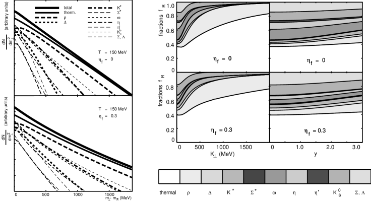
In Fig. 5.1, we plot the pion transverse mass spectrum $dN_{\pi}/dm_{\perp}^{2}$ and the resonance fractions $f_{r}({\rm y},p_{\perp})$ of the model (5.1) for two sets of source parameters. All resonance decay contributions are shown separately. The resonances $\omega$, $\eta$ and $\eta^{\prime}$ contribute with 3-body decays whose decay pions are seen to be particularly concentrated at small $p_{\perp}$. Comparing the cases of vanishing and non-vanishing transverse flow one observes the well-known flattening of the transverse mass spectrum by transverse radial flow [152, 115, 102, 145, 146]. The direct pions reflect essentially an effective “blueshifted” temperature [102]

$$T_{\rm eff}=T\sqrt{{1+\langle\beta_{t}\rangle\over 1-\langle\beta_{t}\rangle}}\,,$$ (5.32)

where the average transverse flow velocity $\langle\beta_{t}\rangle$ is directly related to $\eta_{f}$. This clearly does not allow to separate thermal from collective motion. Deviations from (5.32) are seen for the transverse mass spectra of heavier particles at low $p_{\perp}$ and have been used to determine the temperature and flow velocity separately [136, 158]. One of the main goals of two-particle interferometry is to obtain a more direct measure of the transverse expansion velocity at freeze-out.

5.2.2 Rapidity distribution

The rapidity distribution is given by

$${dN_{\pi}\over d{\rm y}}=\int m_{\perp}dm_{\perp}\,d\phi\int d^{4}x\,S(x;p_{\perp},\phi,{\rm y})\,.$$ (5.33)

For the model (5.1) its width is dominated by the longitudinal width $\Delta\eta$ of the source. This is a consequence of the assumed boost-invariant longitudinal flow profile. Since the resonance decay fractions $f_{r}$ are essentially rapidity independent (see Fig. 5.1), resonance decay contributions do not significantly affect the rapidity spectrum.

5.2.3 Azimuthal dependence

For collisions with non-zero impact parameter the triple-differential one-particle spectrum (3.1.2) contains information about the orientation of the reaction plane. The harmonic coefficients $v_{n}$ which characterize this azimuthal dependence are given in terms of the Fourier transforms [165, 166]

$\displaystyle\left(a_{n},\,b_{n}\right)$ $\displaystyle=$ $\displaystyle{{\int_{0}^{2\pi}E\,{dN\over d^{3}p}\left(\cos(n\phi),\,\sin(n\phi)\right)\,d\phi}\over{\int_{0}^{2\pi}E\,{dN\over d^{3}p}\,d\phi}}\,,$ (5.34)
$\displaystyle a_{n}$ $\displaystyle=$ $\displaystyle v_{n}\,\cos(n\psi_{R})\,,\qquad b_{n}=v_{n}\,\sin(n\psi_{R})\,.$ (5.35)

According to (5.34) they are normalized to the azimuthally averaged double differential particle distribution, and $v_{0}=1$. A symmetry argument similar to that employed in (3.20/3.21) implies that in the limit $p_{\perp}\to 0$ the $\phi$-dependent terms vanish, the emission probabilities in different azimuthal directions become equal, and

$$\lim_{p_{\perp}\to 0}v_{n}(p_{\perp})=0\,\qquad\hbox{for all $n\geq 1$.}$$ (5.36)

Furthermore, the odd harmonic coefficients $v_{n}$ vanish at midrapidity for symmetric collision systems, due to the remaining $\phi\to\phi+\pi$ symmetry in the transverse plane. A more explicit calculation depends on details of the model. For the emission function (5.12)-(5.16) one can show that $v_{2}\propto p_{\perp}^{2}$ for small values of $p_{\perp}$. For small transverse flow, the leading dependence on the anisotropy parameters $\epsilon_{s}$ and $\epsilon_{f}$ is given by

$$v_{2}\propto\eta_{f}^{2}\,{{2(\epsilon_{f}-\epsilon_{s})}\over(1-\epsilon_{f}^{2})\,(1-\epsilon_{s}^{2})}\,.$$ (5.37)

This describes correctly the main features of a numerical study of this model [175]. Both geometric and dynamical deformations manifest themselves in the single-particle spectrum only for expanding sources with $\eta_{f}\neq 0$. The relative minus sign in the numerator of (5.37) reflects the different signs in the definitions of $\epsilon_{s}$ and $\epsilon_{f}$ in (5.13) and (5.15). Once this is taken into account, (5.37) shows that an increasing spatial deformation $\epsilon_{s}$ or an increasing flow anisotropy $\epsilon_{f}$ lead to similar effects on the azimuthal particle distribution. Therefore they cannot be separated without also using information from two-particle correlations.

5.3 Two-particle correlator

In this section we study the question how characteristics of the emission function are reflected in the momentum-dependence of the measured particle correlations. This was discussed already in section  3 in the context of the model-independent relations between the space-time variances of $S(x,K)$ and the HBT radius parameters of $C(\leavevmode\mathchoice{\hbox{\rm tensysevensyfivesy\boldmath{$\displaystyle q$}}}{\hbox{\rm tensysevensyfivesy\boldmath{$\textstyle q$}}}{\hbox{\rm tensysevensyfivesy\boldmath{$\scriptstyle q$}}}{\hbox{\rm tensysevensyfivesy\boldmath{$\scriptscriptstyle q$}}},\leavevmode\mathchoice{\hbox{\rm tensysevensyfivesy\boldmath{$\displaystyle K$}}}{\hbox{\rm tensysevensyfivesy\boldmath{$\textstyle K$}}}{\hbox{\rm tensysevensyfivesy\boldmath{$\scriptstyle K$}}}{\hbox{\rm tensysevensyfivesy\boldmath{$\scriptscriptstyle K$}}})$. According to this discussion spatial and temporal geometric information about the source is contained in the tensysevensyfivesy$\textstyle q$-dependence of the correlator, while the pair momentum dependence characterizes dynamical properties. These statements can be made more explicit in the context of specific model studies.

For quantitatively reliable studies of “realistic” (i.e. sufficiently complex) emission functions the determination of the two-particle correlator requires a numerical evaluation of the Fourier integral in (1.4). On the other hand, simple analytical approximations for the HBT radius parameters allow to summarize the main physical dependencies of the measurable quantities in an intuitive form and are quite useful for a qualitative understanding. We give a combined discussion of both the analytical approximations and the exact numerical results for the model (5.1).

5.3.1 Saddle point approximation of HBT radius parameters

Characterizing the emission function $S(x,K)$ by the Gaussian widths (3.4), $\left(B^{-1}\right)_{\mu\nu}(\leavevmode\mathchoice{\hbox{\rm tensysevensyfivesy\boldmath{$\displaystyle K$}}}{\hbox{\rm tensysevensyfivesy\boldmath{$\textstyle K$}}}{\hbox{\rm tensysevensyfivesy\boldmath{$\scriptstyle K$}}}{\hbox{\rm tensysevensyfivesy\boldmath{$\scriptscriptstyle K$}}})$ $=\langle\tilde{x}_{\mu}\tilde{x}_{\nu}\rangle(\leavevmode\mathchoice{\hbox{\rm tensysevensyfivesy\boldmath{$\displaystyle K$}}}{\hbox{\rm tensysevensyfivesy\boldmath{$\textstyle K$}}}{\hbox{\rm tensysevensyfivesy\boldmath{$\scriptstyle K$}}}{\hbox{\rm tensysevensyfivesy\boldmath{$\scriptscriptstyle K$}}})$, is more generally applicable than a saddle point approximation around its center $\bar{x}(\leavevmode\mathchoice{\hbox{\rm tensysevensyfivesy\boldmath{$\displaystyle K$}}}{\hbox{\rm tensysevensyfivesy\boldmath{$\textstyle K$}}}{\hbox{\rm tensysevensyfivesy\boldmath{$\scriptstyle K$}}}{\hbox{\rm tensysevensyfivesy\boldmath{$\scriptscriptstyle K$}}})$ which was earlier suggested [153, 42]. The tensor $B_{\mu\nu}(\leavevmode\mathchoice{\hbox{\rm tensysevensyfivesy\boldmath{$\displaystyle K$}}}{\hbox{\rm tensysevensyfivesy\boldmath{$\textstyle K$}}}{\hbox{\rm tensysevensyfivesy\boldmath{$\scriptstyle K$}}}{\hbox{\rm tensysevensyfivesy\boldmath{$\scriptscriptstyle K$}}})$ characterizes essential features of the phase-space support of the emission function even if $S(x,K)$ is not differentiable or if its curvature at the saddle point does not represent its average support sufficiently well. In all these cases the Gaussian widths $B_{\mu\nu}(\leavevmode\mathchoice{\hbox{\rm tensysevensyfivesy\boldmath{$\displaystyle K$}}}{\hbox{\rm tensysevensyfivesy\boldmath{$\textstyle K$}}}{\hbox{\rm tensysevensyfivesy\boldmath{$\scriptstyle K$}}}{\hbox{\rm tensysevensyfivesy\boldmath{$\scriptscriptstyle K$}}})$ still translate directly into Gaussian radius parameters, as discussed in section 3. Nevertheless, a saddle point approximation of $S(x,K)$ can be technically useful for the evaluation of the integrals (3.3) when approximating the HBT radius parameters as averages over the emission function [153, 2, 42, 48, 171].

To illustrate the use and limitations of the analytical expressions thus obtained one can study a simplification of the model (5.1) which is particularly amenable to analytical calculations: we neglect the resonance contributions and set $\Delta\eta=\infty$ and $\Delta\tau=0$. This represents a source with exact longitudinal boost-invariance and a sharp freeze-out at time $\tau_{0}$ [42, 153, 171]. For such a source the cross-term $R_{ol}$ vanishes in the LCMS (see (3.17)); it will be discussed in the following subsection.

Expanding the exponent of the emission function $S(x,K)$ given in (5.1) around $x_{\mu}=0$ one obtains in this case

$$-{M_{\perp}\over T}\left(1+{\eta_{f}^{2}\over 2}{{x^{2}+y^{2}}\over R^{2}}\right)-{K_{\perp}\over T}\eta_{f}{x\over R}-{{x^{2}+y^{2}}\over R^{2}}\,.$$ (5.38)

In the saddle point approximation the terms bilinear in $y$ specify the (inverse of the) “side” radius parameter $R_{s}$, while the “outward” radius parameter receives an additional contribution from the finite emission duration $\langle\tilde{t}^{2}\rangle=\tau_{0}^{2}\langle\sinh^{2}\eta\rangle$ according to [42]

$\displaystyle R_{o}^{2}(K_{\perp})$ $\displaystyle=$ $\displaystyle R_{s}^{2}(K_{\perp})+\textstyle{1\over 2}{\left({T\over M_{\perp}}\right)}^{2}{\beta}_{\perp}^{2}{\tau}_{0}^{2}\,,$ (5.39)
$\displaystyle R_{s}^{2}(K_{\perp})$ $\displaystyle=$ $\displaystyle{R^{2}\over 1+{M_{\perp}\over T}\eta_{f}^{2}}\,,$ (5.40)

These simple expressions illustrate several of the key concepts employed in HBT interferometry: the overall size of the transverse radius parameters is determined by the transverse Gaussian widths of the collision region, and the difference $R_{o}^{2}-R_{s}^{2}$ is proportional to the emission duration $\beta_{\perp}^{2}\langle\tilde{t}^{2}\rangle$. (Even a sharp freeze-out at $\tau=\tau_{0}$ corresponds to a finite region in $t=\tau_{0}\cosh\eta$ since the source distribution is sampled over a finite longitudinal range.) Most importantly, however, the radius parameters $R_{o}^{2}$ and $R_{s}^{2}$ are sensitive to the transverse flow strength $\eta_{f}$ of the source: the HBT radius shrinks for finite $\eta_{f}$ since a dynamically expanding source viewed through a filter of wavelength $K$ is seen only partially. This shrinking effect increases for larger values of $M_{\perp}$ proportionally to the ratio $\eta_{f}^{2}/T$. The $M_{\perp}$-dependence of $R_{s}$ is a consequence of transverse position-momentum correlations in the source which here originate from the transverse collective flow.

Saddle point integration also leads to simple expressions for the longitudinal radius parameters. Due to boost-invariance, $R_{l}$ is $\beta_{l}$-independent, and one has to calculate $R_{l}^{2}=\langle\tilde{z}^{2}\rangle$ $=\tau_{0}^{2}\left(\langle\sinh\eta^{2}\rangle-\langle\sinh\eta\rangle^{2}\right)$. We summarize the results for different approximation schemes:

$\displaystyle R_{l}^{2}$ $\displaystyle\approx$ τ02TM,[toO(TM),[106]]superscriptsubscript𝜏02𝑇subscript𝑀perpendicular-toto𝑂𝑇subscript𝑀perpendicular-to[106]\displaystyle{\tau}_{0}^{2}{T\over M_{\perp}}\,,\qquad\qquad\qquad\qquad\qquad\qquad\left[\hbox{to}\,\,O\left(\textstyle{T\over M_{\perp}}\right)\,,\cite[cite]{[\@@bibref{}{MS88}{}{}]}\right] (5.41)
$\displaystyle R_{l}^{2}$ $\displaystyle\approx$ τ02TM(1+(12+11+MTηf2)TM),[toO(T2M2),[42]]superscriptsubscript𝜏02𝑇subscript𝑀perpendicular-to11211subscript𝑀perpendicular-to𝑇superscriptsubscript𝜂𝑓2𝑇subscript𝑀perpendicular-toto𝑂superscript𝑇2subscriptsuperscript𝑀2perpendicular-to[42]\displaystyle\tau_{0}^{2}{T\over M_{\perp}}\,\left(1+\left({1\over 2}+{1\over{1+{M_{\perp}\over T}\eta_{f}^{2}}}\right){T\over M_{\perp}}\right)\,,\left[\hbox{to}\,\,O\left(\textstyle{T^{2}\over M^{2}_{\perp}}\right)\,,\cite[cite]{[\@@bibref{}{CSH95a}{}{}]}\right] (5.42)
Rl2superscriptsubscript𝑅𝑙2\displaystyle R_{l}^{2} =\displaystyle= τ02TMK2(MT)K1(MT).[exact for ηf=0[89]]\displaystyle\tau_{0}^{2}{T\over M_{\perp}}\,{K_{2}({M_{\perp}\over T})\over K_{1}({M_{\perp}\over T})}\,.\qquad\qquad\qquad\hbox{[exact for $\eta_{f}=0$, \cite[cite]{[\@@bibref{}{HB95}{}{}]}]} (5.43)

In general the longitudinal radius is proportional to the average freeze-out time $\tau_{0}$ and falls off strongly with increasing transverse momentum. In this case the transverse momentum dependence signals longitudinal position-momentum correlations in the source. Compared to the transverse directions, it is much stronger since the source expands predominantly in the beam direction.

According to the Makhlin-Sinyukov formula (5.41), fitting an $1/M_{\perp}$-hyperbola to $R_{l}^{2}$ (extracting the temperature e.g. from the one-particle spectrum), the source parameter $\tau_{0}$ can be determined. Early estimates of $\tau_{0}$ have been obtained by this argument. The improved calculations (5.42) and (5.43) show that for realistic temperatures of the order of the pion mass corrections cannot be neglected. Similar remarks apply to the slopes of the “side” and “out” radius parameters (5.39/5.40). Especially, all the results presented here are based on an expansion around $x_{\mu}=0$, while the true saddle point $\bar{x}_{\mu}$ for finite $\eta_{f}$ is shifted in the out-direction; this can be seen from (5.38). In Ref. [171] an approximation scheme was developed which takes these saddle point shifts into account and allows to systematically derive improved expressions for the HBT radii (5.39)-(5.42). The resulting expressions are involved and a numerical evaluation of the radius parameters is often more convenient.

Refer to caption

Figure 5.2: $K_{\perp}$-dependence of the HBT radius parameters $R_{o}$ (a), $R_{s}$ (b) and $R_{l}$ (c) for the emission function (5.1) with $T=150$ MeV, $\tau_{0}=3$ fm/c, $R=3$ fm, $\Delta\eta=\infty$, $\Delta\tau=0$. Curves for different values of the transverse flow $\eta_{f}$ are shown. Differences between numerically evaluated space-time variances and Gaussian widths indicate deviations of $C(\leavevmode\mathchoice{\hbox{\rm tensysevensyfivesy\boldmath{$\displaystyle q$}}}{\hbox{\rm tensysevensyfivesy\boldmath{$\textstyle q$}}}{\hbox{\rm tensysevensyfivesy\boldmath{$\scriptstyle q$}}}{\hbox{\rm tensysevensyfivesy\boldmath{$\scriptscriptstyle q$}}},\leavevmode\mathchoice{\hbox{\rm tensysevensyfivesy\boldmath{$\displaystyle K$}}}{\hbox{\rm tensysevensyfivesy\boldmath{$\textstyle K$}}}{\hbox{\rm tensysevensyfivesy\boldmath{$\scriptstyle K$}}}{\hbox{\rm tensysevensyfivesy\boldmath{$\scriptscriptstyle K$}}})$ from a Gaussian shape. Differences to the dash-dotted lines reflect the limited validity of a naive saddle point approximation around $x_{\mu}=0$.

The sources for quantitative uncertainties of the saddle point approximation are two-fold: The determination of the saddle point $\bar{x}_{\mu}=\langle x_{\mu}\rangle$ is done only approximately in many model studies. The resulting inaccuracies turn out to be substantial and put severe limitations on the quantitative applicability of the analytical expressions quoted above. This is illustrated in Fig. 5.2. Moreover, whenever the Gaussian widths of the correlator deviate significantly from its curvature at $\leavevmode\mathchoice{\hbox{\rm tensysevensyfivesy\boldmath{$\displaystyle q$}}}{\hbox{\rm tensysevensyfivesy\boldmath{$\textstyle q$}}}{\hbox{\rm tensysevensyfivesy\boldmath{$\scriptstyle q$}}}{\hbox{\rm tensysevensyfivesy\boldmath{$\scriptscriptstyle q$}}}=0$, the relation between space-time variances and HBT-radii becomes quantitatively unreliable, see chapter 4. In the following we therefore use the above simple analytical expressions only for qualitative guidance, basing a quantitative discussion on numerical results.

Equations (5.39)-(5.43) have been used to extract the transverse flow parameter $\eta_{f}$ and the “freeze-out time” $\tau_{0}$. This is not without danger. As pointed out in Ref. [42], in this particular model the $M_{\perp}$-dependence of the HBT radius parameters reflects the longitudinal and transverse flow velocity gradients. These are responsible for the reduced homogeneity lengths compared to the total source size. The parameter $\eta_{f}^{2}$ in (5.40) really reflects the transverse flow velocity gradient [42], and the parameter $\tau_{0}^{2}$ in (5.41)-(5.43) similarly arises from the longitudinal velocity gradient at freeze-out. From the general considerations of section 3.1 we know that the absolute position of the source in space and time cannot be measured. Therefore, strictly speaking, $\tau_{0}$ cannot be directly associated with the absolute freeze-out time. Such an interpretation of $\tau_{0}$ makes the additional dynamical assumption that the longitudinally boost-invariant velocity profile existed not only at the point of freeze-out but throughout the dynamical evolution of the reaction zone. If this were not the case and the collision region underwent, for example, longitudinal acceleration before freeze-out, the real time interval between impact and freeze-out would be longer.

5.3.2 The out-longitudinal cross-term

The cross-term $R_{ol}^{2}$ of the Cartesian parametrization vanishes in the LCMS for longitudinally boost-invariant systems or in symmetric collisions at mid-rapidity. This follows from the corresponding space-time variance (3.13) which vanishes in the LCMS if the source is symmetric under $\tilde{z}\to-\tilde{z}$. This reflection symmetry is broken, however, in the forward and backward rapidity regions for the systems with finite longitudinal extension.

Refer to caption

Figure 5.3: Left: Contour plot of the correlation function in the $q_{o}$-$q_{l}$-plane obtained by NA35 in S+Au collisions at 200 A GeV. The data are for forward rapidity pairs, $3.5<Y<4.5$, the momentum differences are evaluated in a system at rapidity 3. (Figure taken from [3].) Right: $M_{\perp}$-dependence of the out-longitudinal radius parameter for the model (5.1) at $Y_{\rm cm}=1.5$ in the LCMS. The curves are shown for different values of the transverse flow, $\eta_{f}=0.4$ (solid) and $\eta_{f}=1.0$ (dashed). (Figure taken from [163].)

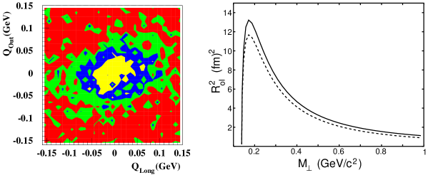
As first observed by NA35 [3], following a proposal of Chapman et al. [41, 43], the Gaussian correlator is then an ellipsoid in tensysevensyfivesy$\textstyle q$-space whose main axes do not coincide with the Cartesian ones: it is tilted in the out-longitudinal plane (see the l.h.s. of Fig. 5.3). This tilt is parametrized by the size and sign of $R_{ol}^{2}$. In the forward rapidity region, $R_{ol}^{2}$ is positive in the LCMS and negative in the CMS [43, 13, 147]. The sign is reversed for the backward rapidity region.

Also, $R_{ol}^{2}$ has a characteristic transverse momentum dependence. At vanishing $K_{\perp}$, the $\tilde{x}\to-\tilde{x}$ symmetry of the source is restored and $R_{ol}^{2}$ vanishes, see (3.21) and the l.h.s. of Fig. 5.3. At large $K_{\perp}$, on the other hand, the homogeneity region peaks sharply around the point of highest emissivity, and the $\tilde{z}\to-\tilde{z}$ symmetry is again approximately restored [180]. The resulting generic $M_{\perp}$ dependence is seen in Fig. 5.3: $|R_{ol}^{2}|$ rises sharply at small $K_{\perp}$, reaches a maximum and then decreases again.

5.3.3 The Yano-Koonin velocity

The Yano-Koonin-Podgoretskiĭ parametrization [182, 123, 79, 180] describes the correlator of an azimuthally symmetric source by a longitudinal velocity $v(\leavevmode\mathchoice{\hbox{\rm tensysevensyfivesy\boldmath{$\displaystyle K$}}}{\hbox{\rm tensysevensyfivesy\boldmath{$\textstyle K$}}}{\hbox{\rm tensysevensyfivesy\boldmath{$\scriptstyle K$}}}{\hbox{\rm tensysevensyfivesy\boldmath{$\scriptscriptstyle K$}}})$ and three Gaussian radius parameters $R_{\perp}^{2}(\leavevmode\mathchoice{\hbox{\rm tensysevensyfivesy\boldmath{$\displaystyle K$}}}{\hbox{\rm tensysevensyfivesy\boldmath{$\textstyle K$}}}{\hbox{\rm tensysevensyfivesy\boldmath{$\scriptstyle K$}}}{\hbox{\rm tensysevensyfivesy\boldmath{$\scriptscriptstyle K$}}})$, $R_{\parallel}^{2}(\leavevmode\mathchoice{\hbox{\rm tensysevensyfivesy\boldmath{$\displaystyle K$}}}{\hbox{\rm tensysevensyfivesy\boldmath{$\textstyle K$}}}{\hbox{\rm tensysevensyfivesy\boldmath{$\scriptstyle K$}}}{\hbox{\rm tensysevensyfivesy\boldmath{$\scriptscriptstyle K$}}})$, and $R_{0}^{2}(\leavevmode\mathchoice{\hbox{\rm tensysevensyfivesy\boldmath{$\displaystyle K$}}}{\hbox{\rm tensysevensyfivesy\boldmath{$\textstyle K$}}}{\hbox{\rm tensysevensyfivesy\boldmath{$\scriptstyle K$}}}{\hbox{\rm tensysevensyfivesy\boldmath{$\scriptscriptstyle K$}}})$. The Yano-Koonin velocity $v(\leavevmode\mathchoice{\hbox{\rm tensysevensyfivesy\boldmath{$\displaystyle K$}}}{\hbox{\rm tensysevensyfivesy\boldmath{$\textstyle K$}}}{\hbox{\rm tensysevensyfivesy\boldmath{$\scriptstyle K$}}}{\hbox{\rm tensysevensyfivesy\boldmath{$\scriptscriptstyle K$}}})$ contains important information about the longitudinal expansion of the source. To investigate this, a detailed study [180] was done within the framework of the class of models (5.1), of the relation among the following different longitudinal reference frames:

  • CMS: The centre of mass frame of the fireball, specified by $\eta_{0}=0$.

  • LCMS (Longitudinally CoMoving System [50]): a pair-dependent frame, specified by $\beta_{l}=Y=0$. In this frame, only the transverse velocity component of the particle pair is non-vanishing.

  • LSPS (Longitudinal Saddle-Point System [48]): The longitudinally moving rest frame of the point of maximal emissivity for a given pair momentum. In general, the velocity of this frame depends on the momentum of the emitted particle pair. For symmetric sources the point of maximal emissivity (“saddle point”) coincides with the “source centre” $\bar{x}(\leavevmode\mathchoice{\hbox{\rm tensysevensyfivesy\boldmath{$\displaystyle K$}}}{\hbox{\rm tensysevensyfivesy\boldmath{$\textstyle K$}}}{\hbox{\rm tensysevensyfivesy\boldmath{$\scriptstyle K$}}}{\hbox{\rm tensysevensyfivesy\boldmath{$\scriptscriptstyle K$}}})$ defined in (3.2). In this approximation, for a source like (5.1), the LSPS velocity is given by the longitudinal component of $u^{\mu}(\bar{x}(\leavevmode\mathchoice{\hbox{\rm tensysevensyfivesy\boldmath{$\displaystyle K$}}}{\hbox{\rm tensysevensyfivesy\boldmath{$\textstyle K$}}}{\hbox{\rm tensysevensyfivesy\boldmath{$\scriptstyle K$}}}{\hbox{\rm tensysevensyfivesy\boldmath{$\scriptscriptstyle K$}}}))$.

  • YK (Yano-Koonin frame [79]): The frame for which the YKP velocity parameter vanishes, $v(\leavevmode\mathchoice{\hbox{\rm tensysevensyfivesy\boldmath{$\displaystyle K$}}}{\hbox{\rm tensysevensyfivesy\boldmath{$\textstyle K$}}}{\hbox{\rm tensysevensyfivesy\boldmath{$\scriptstyle K$}}}{\hbox{\rm tensysevensyfivesy\boldmath{$\scriptscriptstyle K$}}})=0$. Again, this frame is in general pair momentum dependent.

The velocities (or rapidities) of the CMS and LCMS frames can be determined experimentally, the first from the peak in the single particle rapidity distribution, the second from the longitudinal momentum of the measured pion pair. The velocity of the LSPS is determined by the flow velocity at $\bar{x}(\leavevmode\mathchoice{\hbox{\rm tensysevensyfivesy\boldmath{$\displaystyle K$}}}{\hbox{\rm tensysevensyfivesy\boldmath{$\textstyle K$}}}{\hbox{\rm tensysevensyfivesy\boldmath{$\scriptstyle K$}}}{\hbox{\rm tensysevensyfivesy\boldmath{$\scriptscriptstyle K$}}})$ and hence, it is not directly measurable (neither the one- nor the two-particle spectra depend on $\bar{x}(\leavevmode\mathchoice{\hbox{\rm tensysevensyfivesy\boldmath{$\displaystyle K$}}}{\hbox{\rm tensysevensyfivesy\boldmath{$\textstyle K$}}}{\hbox{\rm tensysevensyfivesy\boldmath{$\scriptstyle K$}}}{\hbox{\rm tensysevensyfivesy\boldmath{$\scriptscriptstyle K$}}})$). However, the YK- and LSPS-systems coincide as long as the particle emission is symmetric around $\bar{x}(\leavevmode\mathchoice{\hbox{\rm tensysevensyfivesy\boldmath{$\displaystyle K$}}}{\hbox{\rm tensysevensyfivesy\boldmath{$\textstyle K$}}}{\hbox{\rm tensysevensyfivesy\boldmath{$\scriptstyle K$}}}{\hbox{\rm tensysevensyfivesy\boldmath{$\scriptscriptstyle K$}}})$ [123, 180].

Refer to caption


Figure 5.4: Calculation of the Yano-Koonin rapidity for the model (5.1) without resonances. Source parameters: $R=3$ fm, $\tau_{0}=3$ fm/c, $\Delta\tau=1$ fm/c, $\Delta\eta=1.2$ and $T=140$ MeV. (a) YK rapidity as a function of the pion pair rapidity $Y$ (both measured in the CMS frame of the source), for various values of the transverse pair momentum $K_{\perp}$ and for two values of the transverse flow rapidity $\eta_{f}$. (b) Same as (a), but shown as a function of $K_{\perp}$ for different values of $Y$. The curves for negative $Y$ are obtained by reflection along the abscissa. (c) The difference $Y_{{}_{\rm YK}}-Y_{{}_{\rm LSPS}}$ between the rapidity of the YK frame and the longitudinal rest system of the saddle point, plotted in the same way as (a). (d) Same as (c), but shown as a function of $K_{\perp}$ for different values of $Y$.

In model studies based on the parametrization (5.1) asymmetries are found to be small [180]. This is seen in the difference between the corresponding rapidities, $Y_{{}_{\rm YK}}-Y_{{}_{\rm LSPS}}$, plotted in Figure 5.4c,d as a function of $K_{\perp}$ and $Y$ respectively. The difference is generally small, especially for large transverse momenta [79, 180] where thermal smearing can be neglected:

$$v(\leavevmode\mathchoice{\hbox{\rm tensysevensyfivesy\boldmath{$\displaystyle K$}}}{\hbox{\rm tensysevensyfivesy\boldmath{$\textstyle K$}}}{\hbox{\rm tensysevensyfivesy\boldmath{$\scriptstyle K$}}}{\hbox{\rm tensysevensyfivesy\boldmath{$\scriptscriptstyle K$}}})\approx v_{{}_{\rm LSPS}}(\leavevmode\mathchoice{\hbox{\rm tensysevensyfivesy\boldmath{$\displaystyle K$}}}{\hbox{\rm tensysevensyfivesy\boldmath{$\textstyle K$}}}{\hbox{\rm tensysevensyfivesy\boldmath{$\scriptstyle K$}}}{\hbox{\rm tensysevensyfivesy\boldmath{$\scriptscriptstyle K$}}})\,.$$ (5.44)

The observable YK velocity thus tracks the unobservable LSPS velocity. This is important since longitudinal expansion of the source leads to a characteristic dependence of the LSPS velocity $v_{{}_{\rm LSPS}}$ on the pair rapidity which - using (5.44) - one can confirm by measuring the YK-velocity. Two extreme examples illustrate this: for a static source without position-momentum correlations the rapidity of the LSPS is independent of the pair rapidity $Y$ and identical to the rapidity of the CMS:

$$Y_{{}_{\rm LSPS}}=\frac{1}{2}\ln{1+v_{{}_{\rm LSPS}}\over 1-v_{{}_{\rm LSPS}}}={\rm const.}\ \ \ \hbox{ for a static source.}$$ (5.45)

In contrast, for a longitudinally boost-invariant model (5.1) with $\Delta\eta=\infty$, the longitudinal saddle point lies at $\eta=Y$. In this case, the LSPS and the LCMS coincide,

$$Y_{{}_{\rm LSPS}}=\eta=Y\,\qquad\hbox{ for a longitudinal boost-invariant source.}$$ (5.46)

For the model (5.1) the measurable YK rapidity $Y_{{}_{\rm YK}}$ is plotted in Figure 5.4a,b as a function of the longitudinal pair rapidity $Y$ and transverse momentum $K_{\perp}$. The plot confirms a linear relation

YYKconst.×Y, for the model (5.1).Y_{{}_{\rm YK}}\approx{\rm const.}\,\times\,Y\,,\qquad\hbox{ for the model~{}(\ref{5.1}).} (5.47)

with a proportionality constant which approaches unity for large $K_{\perp}$. Since $Y_{{}_{\rm YK}}\approx Y_{\rm LSPS}$, this linear relation between the rapidity $Y_{{}_{\rm YK}}$ of the Yano-Koonin frame and the pion pair rapidity $Y$ is a direct reflection of the longitudinal expansion flow. The linear relation shown in Fig. 5.4a has been confirmed subsequently by experiment [13]. There are also first experimental hints for the $K_{\perp}$-dependence shown in 5.4a.

We emphasize that the observation of a linear relation $Y_{{}_{\rm YK}}=Y$ cannot be generally interpreted as evidence for boost-invariant longitudinal expansion, as was suggested in Refs. [79, 180, 78]. In Fig. 5.4a one sees that for the model (5.1) this linear relation is the better satisfied the larger the transverse momentum of the particle pair. This can be easily understood as a consequence of the reduced thermal smearing at large $K_{\perp}$. Whenever the random component in the momentum distribution becomes small, the observed pair velocities track directly the flow velocity of the emitting volume element, irrespective of the actual flow velocity profile. The generic behaviour shown in Fig. 5.4a therefore indicates longitudinal expansion which is sufficiently strong to overcome the thermal smearing, but not necessarily boost-invariant.

5.3.4 Yano-Koonin-Podgoretskiĭ radius parameters

We discussed in section 3.2 that, as long as certain asymmetries of the source are negligible, the YKP-radius parameters have a particularly simple space-time interpretation. The transverse radius parameter always coincides with the source width in the side-direction, $R_{\perp}^{2}(\leavevmode\mathchoice{\hbox{\rm tensysevensyfivesy\boldmath{$\displaystyle K$}}}{\hbox{\rm tensysevensyfivesy\boldmath{$\textstyle K$}}}{\hbox{\rm tensysevensyfivesy\boldmath{$\scriptstyle K$}}}{\hbox{\rm tensysevensyfivesy\boldmath{$\scriptscriptstyle K$}}})=\langle\tilde{y}^{2}\rangle$, and [79, 180]

$\displaystyle R_{\parallel}^{2}(\leavevmode\mathchoice{\hbox{\rm tensysevensyfivesy\boldmath{$\displaystyle K$}}}{\hbox{\rm tensysevensyfivesy\boldmath{$\textstyle K$}}}{\hbox{\rm tensysevensyfivesy\boldmath{$\scriptstyle K$}}}{\hbox{\rm tensysevensyfivesy\boldmath{$\scriptscriptstyle K$}}})$ $\displaystyle=$ $\displaystyle\left\langle\left(\tilde{z}-{\beta_{l}\over\beta_{\perp}}\tilde{x}\right)^{2}\right\rangle-{\beta_{l}^{2}\over\beta_{\perp}^{2}}\langle\tilde{y}^{2}\rangle\approx\langle\tilde{z}^{2}\rangle\,,$ (5.48)
$\displaystyle R_{0}^{2}(\leavevmode\mathchoice{\hbox{\rm tensysevensyfivesy\boldmath{$\displaystyle K$}}}{\hbox{\rm tensysevensyfivesy\boldmath{$\textstyle K$}}}{\hbox{\rm tensysevensyfivesy\boldmath{$\scriptstyle K$}}}{\hbox{\rm tensysevensyfivesy\boldmath{$\scriptscriptstyle K$}}})$ $\displaystyle=$ $\displaystyle\left\langle\left(\tilde{t}-{1\over\beta_{\perp}}\tilde{x}\right)^{2}\right\rangle-{1\over\beta_{\perp}^{2}}\langle\tilde{y}^{2}\rangle\approx\langle\tilde{t}^{2}\rangle\,.$ (5.49)

Refer to caption

Figure 5.5: YKP radii for the same model as in Fig. 5.4. (a) $R_{0}$ and $\sqrt{\langle\tilde{t}^{2}\rangle}$, evaluated in the YK frame, as a function of $M_{\perp}$ for three values of the transverse flow rapidity $\eta_{f}$, for pion pairs with CMS rapidity $Y=0$. (b) Same as (a), but for pions with CMS rapidity $Y=3$. (c) and (d): Same as (a) and (b), but for $R_{\parallel}$ and the longitudinal length of homogeneity $\sqrt{\langle\tilde{z}^{2}\rangle}$, evaluated in the YK frame. For $Y=0$, $R_{\parallel}$ and $\sqrt{\langle\tilde{z}^{2}\rangle}$ agree exactly because $\beta_{l}=0$ in the YK frame.

The approximation in these equations results from dropping terms proportional to $\langle\tilde{z}\tilde{x}\rangle$, $\langle\tilde{x}\tilde{t}\rangle$, and $\langle\tilde{x}^{2}-\tilde{y}^{2}\rangle$. The first two of these terms vanish if the source is symmetric around its point of highest emissivity $\bar{x}(\leavevmode\mathchoice{\hbox{\rm tensysevensyfivesy\boldmath{$\displaystyle K$}}}{\hbox{\rm tensysevensyfivesy\boldmath{$\textstyle K$}}}{\hbox{\rm tensysevensyfivesy\boldmath{$\scriptstyle K$}}}{\hbox{\rm tensysevensyfivesy\boldmath{$\scriptscriptstyle K$}}})$. In Figure 5.5 the effective emission duration $\sqrt{\langle\tilde{t}^{2}\rangle}$ and longitudinal size of homogeneity $\sqrt{\langle\tilde{z}^{2}\rangle}$ are compared to $R_{0}$ and $R_{\parallel}$ for the model (5.1). The approximations (5.48/5.49) become exact for vanishing transverse flow while differences occur especially in $R_{0}$ for large $K_{\perp}$ or significant transverse flow. These can be traced to the terms $-2\langle\tilde{x}\tilde{t}\rangle/\beta_{\perp}+\langle\tilde{x}^{2}-\tilde{y}^{2}\rangle/\beta_{\perp}^{2}$ which are neglected in (5.49). For the model (5.1) the space-time variances $\langle\tilde{x}\tilde{t}\rangle$ and $\langle\tilde{x}^{2}-\tilde{y}^{2}\rangle$ indeed vanish for $K_{\perp}\to 0$ where the azimuthal $x$-$y$-symmetry of the source is restored. However, when divided by powers of $\beta_{\perp}$, the corresponding terms in (5.49) result in small but finite contributions even for $K_{\perp}\to 0$. For opaque sources (5.9) the term $-2\langle\tilde{x}\tilde{t}\rangle/\beta_{\perp}+\langle\tilde{x}^{2}-\tilde{y}^{2}\rangle/\beta_{\perp}^{2}$ can be the dominant contribution; this can lead to large negative values of $R_{0}^{2}(K_{\perp})$. The approximation (5.49) thus breaks down for such opaque sources [84, 160, 161], and the leading $K_{\perp}$-dependence can be recast in the approximate expression (3.58). The experimental data exclude large negative values for $R_{0}^{2}(K_{\perp})$ and thus rule out certain opaque emission functions [160, 177, 161].

5.3.5 Azimuthal dependence of HBT radius parameters

Both the calculation of HBT-radius parameters in the saddle-point approximation and the numerical calculation have been extended [175] to the finite impact parameter model described in (5.12)-(5.16). For this model the first harmonics vanish, and the zeroth and second harmonics can be written in the saddle point approximation in terms of an average size $\bar{R}$ and a dimensionless anisotropy parameter $\tilde{\alpha}_{2}$:

Refer to caption

Figure 5.6: First (upper panel, $R_{*,1}^{2}$) and second (lower panel, $R_{*,2}^{2}$) harmonic coefficients of the transverse HBT radius parameters of the model (5.18)/(5.19) and the model (5.14)/(5.15), respectively. The subscript “$*$” in $R_{*,1}^{2}$, $R_{*,2}^{2}$ stands for the out (dash-dotted), side (dashed) and out-side (dotted) components. Solid thin and thick lines denote the zeroth harmonics of the out and side radius parameters, respectively. All calculations are for $T=150$ MeV, $\tau_{0}=5$ fm/c, $\Delta\tau=1$ fm/c, $\Delta\eta=1.2$ and $R=5$ fm.
$\displaystyle{R_{o,0}}^{2}$ $\displaystyle=$ $\displaystyle\bar{R}^{2}+\beta_{\perp}^{2}\langle\tilde{t}^{2}\rangle\,,\qquad{R_{s,0}}^{2}=\bar{R}^{2}\,,$ (5.50)
$\displaystyle{R_{o,2}^{c}}^{2}$ $\displaystyle=$ $\displaystyle-{R_{s,2}^{c}}^{2}=-{R_{os,2}^{s}}^{2}=\tilde{\alpha}_{2}\bar{R}^{2}\,.$ (5.51)

$\tilde{\alpha}_{2}$ is related to the parameter $\alpha_{2}$ in (3.30) by $\alpha_{2}=\tilde{\alpha}_{2}\bar{R}^{2}$. According to (5.51) the relations (3.30) are exact in the saddle point approximation, with

$\displaystyle\bar{R}^{2}$ $\displaystyle=$ $\displaystyle{R^{2}\left({1+\textstyle{M_{\perp}\over T}\eta_{f}^{2}\,(1-\epsilon_{s}^{2})}\right)\over{1+2\textstyle{M_{\perp}(1-\epsilon_{s}\epsilon_{f})\over T}\eta_{f}^{2}+\textstyle{M_{\perp}^{2}(1-\epsilon_{s}^{2})\,(1-\epsilon_{f}^{2})\over T^{2}}\eta_{f}^{4}}}\,,$ (5.52)
$\displaystyle\tilde{\alpha}_{2}$ $\displaystyle=$ $\displaystyle-{\epsilon_{s}\over 2}{{1+\textstyle{\epsilon_{f}\over\epsilon_{s}}\,\textstyle{M_{\perp}\over T}\eta_{f}^{2}\,(1-\epsilon_{s}^{2})}\over{1+\textstyle{M_{\perp}\over T}\eta_{f}^{2}(1-\epsilon_{s}^{2})}}\,.$ (5.53)

For vanishing anisotropy $\epsilon_{s}=\epsilon_{f}=0$ the side radius parameter in (5.52) reduces to the corresponding expression (5.40). For non-zero $\epsilon_{s}$ or $\epsilon_{f}$ the average size $\bar{R}$ depends only weakly on these anisotropies.

In Figure 5.6 we show the results of a numerical study of the model (5.14/5.15) which qualitatively confirms the results of the saddle-point approximation. The deviations from the leading dependence ${R_{o,2}^{c}}^{2}\,:\,{R_{s,2}^{c}}^{2}\,:\,-{R_{os,2}^{s}}^{2}$ $=1\,:\,-1\,:\,-1$ of (5.51) are seen to be small. Similarly, the numerical study of the model (5.18/5.19) which includes directed transverse flow in the forward rapidity region allows to confirm the relation (3.29) between the first harmonic coefficients, ${R_{o,1}^{c}}^{2}\,:\,{R_{s,1}^{c}}^{2}\,:\,{R_{os,1}^{s}}^{2}$ $=3\,:\,1\,:\,-1$.

5.3.6 Resonance decay contributions

Resonance decay pions affect the two-particle correlator by reducing its intercept $\lambda(\leavevmode\mathchoice{\hbox{\rm tensysevensyfivesy\boldmath{$\displaystyle K$}}}{\hbox{\rm tensysevensyfivesy\boldmath{$\textstyle K$}}}{\hbox{\rm tensysevensyfivesy\boldmath{$\scriptstyle K$}}}{\hbox{\rm tensysevensyfivesy\boldmath{$\scriptscriptstyle K$}}})$ and by changing its tensysevensyfivesy$\textstyle q$-dependence. Typical examples are shown in Fig. 5.7. The modifications of $C(\leavevmode\mathchoice{\hbox{\rm tensysevensyfivesy\boldmath{$\displaystyle q$}}}{\hbox{\rm tensysevensyfivesy\boldmath{$\textstyle q$}}}{\hbox{\rm tensysevensyfivesy\boldmath{$\scriptstyle q$}}}{\hbox{\rm tensysevensyfivesy\boldmath{$\scriptscriptstyle q$}}},\leavevmode\mathchoice{\hbox{\rm tensysevensyfivesy\boldmath{$\displaystyle K$}}}{\hbox{\rm tensysevensyfivesy\boldmath{$\textstyle K$}}}{\hbox{\rm tensysevensyfivesy\boldmath{$\scriptstyle K$}}}{\hbox{\rm tensysevensyfivesy\boldmath{$\scriptscriptstyle K$}}})$ due to resonance decays are a consequence of the exponential decay law in (5.28), which provides the emission function $S_{r\to\pi}$ with a non-Gaussian tail in coordinate space.

Refer to caption


Figure 5.7: Two-pion correlations for the model (5.1) without transverse flow ($\eta_{f}=0$), calculated according to (5.20). Curves show the correlator without resonance contributions (thin solid lines), including pions from $\rho$ decays (long-dashed), other shortlived resonances $\Delta$, $K^{*}$, $\Sigma^{*}$ (short-dashed), from the $\omega$ (dash-dotted), and including pions from the longlived resonances $\eta$, $\eta^{\prime}$, $K_{S}^{0}$, $\Sigma$, $\Lambda$ (thick solid lines).

The latter is reflected in a non-Gaussian shape of the correlator. The details depend on the lifetime of the corresponding parent resonances [172]:

  • Short-lived resonances, $\Gamma>30$ MeV: In the rest frame of the particle emitting fluid element these resonances decay very close to their production point, especially if they are heavy and have only small thermal velocities. This means that the emission function $S_{r\to\pi}$ of the daughter pions has a very similar spatial structure as that of the parent resonance, $S_{r}^{\rm dir}$, although at a shifted momentum and shifted in time by the lifetime of the resonance. Since the Fourier transform of the direct emission function is rather Gaussian and the decay pions from short-lived resonances appear close to the emission point of the parent, they maintain the Gaussian features of the correlator.

  • Long-lived resonances, $\Gamma\ll 1$ MeV: These are mainly the $\eta$ and $\eta^{\prime}$, with lifetimes $c\tau\approx 17.000$ and $1000$ fm, respectively, and the weak decays of $K_{S}^{0}$ and the hyperons which on average propagate several cm. Even with thermal velocities these particles travel far outside the direct emission region before decaying, generating a daughter pion emission function $S_{r\to\pi}$ with a very large spatial support. The Fourier transform $\tilde{S}_{r\to\pi}(q,K)$ thus decays very rapidly for $q\neq 0$, giving no contribution in the experimentally accessible region $q>1$ MeV. (This lower limit in $q$ arises from the finite two-track resolution in the experiments.) The decay pions do, however, contribute to the single particle spectrum $\tilde{S}_{r\to\pi}(q=0,K)$ in the denominator and thus “dilute” the correlation. In this way long-lived resonances decrease the correlation strength $\lambda$ without affecting the shape of the correlator where it can be measured.

  • Moderately long-lived resonances, $1$ MeV $<\Gamma<30$ MeV. There is only one such resonance, the $\omega$ meson. It is not sufficiently long-lived to escape detection in the correlator, and thus it does not affect the intercept parameter $\lambda$. Its lifetime is, however, long enough to cause a long exponential tail in $S_{\omega\to\pi}(x,K)$. This seriously distorts the shape of the correlator and destroys its Gaussian form.

The main effects of resonance decay contributions on the $\lambda$ intercept parameter are mimicked by the “core-halo-model” [49] which assumes that the emission function can be written as a sum of two contributions

$$S(x,K)=S_{c}(x,K)+S_{h}(x,K)\,.$$ (5.54)

Here, the “halo” source function $S_{h}$ is regarded as the sum over the longlived resonance contributions which are wide enough to be unresolvable by HBT measurements. $S_{h}$ thus affects only the intercept parameter. The “core” emission function describes the contributions from the direct pions and shortlived resonance decay pions which are emitted from the same central region. The model (5.54) is thus a simplified version of (5.20) and provides a simple qualitative picture for the intercept:

$$\lambda(K)\approx\left(1-\sum_{r={\rm longlived}}f_{r}(K)\right)^{2}\,.$$ (5.55)

The core-halo model neglects contributions from moderately longlived resonances, essentially the $\omega$, for which the distinction into core and halo does not apply. Due to their non-Gaussian shape these affect the fit parameters for the intercept $\lambda$ considerably and can lead to quantitative corrections of (5.55) of up to 10 % [172]. An important consequence following already from (5.55) is the transverse flow dependence of the intercept parameter, depicted in Figure 5.8. With increasing transverse flow, the $K_{\perp}$-dependence of the $\lambda$-parameter becomes flatter [164], though it does not vanish (see Fig. 5.8). This is important since current measurements are consistent with a $K_{\perp}$-independent intercept parameter [24, 13, 147].

Refer to caption


Figure 5.8: The intercept parameter as a function of $M_{\perp}$ for different transverse flow strengths $\eta_{f}$. We use the model (5.1) with temperature $T=150MeV$. The calculation is not based on a proper fit of the two-particle correlation function, but on (5.55), including in the sum over resonances the contributions from $\omega$, $\eta$, $\eta^{\prime}$, and $K_{S}^{0}$.

Aside from this (model-independent) lifetime effect, which generically increases the effective pion emission region, various model-dependent features can affect the degree to which resonance decay contributions change the shape of the correlator. In the model (5.1) for example, the size of the effective emission region in the transverse plane shrinks with increasing transverse flow $\eta_{f}$ approximately according to (5.40). The simplified core-halo model [49] neglects the proper resonance decay kinematics and thus does not describe this effect. As a consequence, the direct resonance emission function $S_{r}^{\rm dir}$ in (5.1) has a smaller effective emission region than that of the thermal pions, due to the larger transverse mass $M_{\perp}$ of the parent resonance (“transverse flow effect”). For finite transverse flow this reduces the size of the resonance emission region and counteracts the lifetime effect. Other models of heavy ion collisions [141, 143] do not show this behaviour and lead to significantly different tensysevensyfivesy$\textstyle q$-dependences of the correlator.

5.3.7 Kurtosis of the correlator

If, as in the presence of resonance decays, the correlator deviates from a Gaussian shape, the characterization of $C(\leavevmode\mathchoice{\hbox{\rm tensysevensyfivesy\boldmath{$\displaystyle q$}}}{\hbox{\rm tensysevensyfivesy\boldmath{$\textstyle q$}}}{\hbox{\rm tensysevensyfivesy\boldmath{$\scriptstyle q$}}}{\hbox{\rm tensysevensyfivesy\boldmath{$\scriptscriptstyle q$}}},\leavevmode\mathchoice{\hbox{\rm tensysevensyfivesy\boldmath{$\displaystyle K$}}}{\hbox{\rm tensysevensyfivesy\boldmath{$\textstyle K$}}}{\hbox{\rm tensysevensyfivesy\boldmath{$\scriptstyle K$}}}{\hbox{\rm tensysevensyfivesy\boldmath{$\scriptscriptstyle K$}}})$ via HBT radius parameters is not unambiguous. Fit results then depend on the relative momentum region covered by the data, on the statistical weights of the different tensysevensyfivesy$\textstyle q$-bins, and on details of the fitting procedure.

The $q$-moments discussed in section 4.2 allow to quantify deviations of the correlator from a Gaussian shape [173, 98]. They are sensitive to differences between model scenarios which cannot be distinguished on the basis of Gaussian radius parameters. To illustrate this point we show in Figure 5.9 both the side radius parameter $R_{s}(\leavevmode\mathchoice{\hbox{\rm tensysevensyfivesy\boldmath{$\displaystyle K$}}}{\hbox{\rm tensysevensyfivesy\boldmath{$\textstyle K$}}}{\hbox{\rm tensysevensyfivesy\boldmath{$\scriptstyle K$}}}{\hbox{\rm tensysevensyfivesy\boldmath{$\scriptscriptstyle K$}}}_{\perp})$ and the corresponding one-dimensional kurtosis $\Delta_{s}(\leavevmode\mathchoice{\hbox{\rm tensysevensyfivesy\boldmath{$\displaystyle K$}}}{\hbox{\rm tensysevensyfivesy\boldmath{$\textstyle K$}}}{\hbox{\rm tensysevensyfivesy\boldmath{$\scriptstyle K$}}}{\hbox{\rm tensysevensyfivesy\boldmath{$\scriptscriptstyle K$}}}_{\perp})$, calculated according to (4.13) and (4.16). In the present case, the side radius parameter calculated from the inverted second $q$-moment coincides rather accurately with the radius parameters extracted from a fit to

$$\tilde{C}(q_{i},\leavevmode\mathchoice{\hbox{\rm tensysevensyfivesy\boldmath{$\displaystyle K$}}}{\hbox{\rm tensysevensyfivesy\boldmath{$\textstyle K$}}}{\hbox{\rm tensysevensyfivesy\boldmath{$\scriptstyle K$}}}{\hbox{\rm tensysevensyfivesy\boldmath{$\scriptscriptstyle K$}}})=1\,+\,\lambda\,e^{-R_{i}^{2}q_{i}^{2}}\,,\qquad\,i=o,s,l$$ (5.56)

in the range $q_{i}\leq 100$ MeV. For a transverse flow between $\eta_{f}=0$ and $\eta_{f}=0.3$, $R_{s}$ shows approximately the same $K_{\perp}$-slope. Hence, once resonance decays are taken into account, scenarios with and without transverse flow cannot be distinguished unambiguously on the basis of (5.40). The physical origin of the $K_{\perp}$-slope of $R_{s}$ is, however, different in the two situations, and this shows up in the kurtosis of the correlator. Without transverse flow, resonance decay contributions increase $R_{s}$ due to the lifetime effect. For non-zero transverse flow, on the other hand, the $K_{\perp}$-slope arises from the $K_{\perp}$-dependent shrinking (5.40) of the effective transverse emission region which is more prominent for resonances than for thermal pions. $S_{\pi}^{\rm dir}$ is spatially more extended in the transverse plane than $S_{R}^{\rm dir}$, and thus “covers” a substantial part of the exponential tails of $S_{R\to\pi}$ [172]. As a consequence, the total emission function (5.20) shows much smaller deviations from a Gaussian shape for the scenario with transverse flow and results in a more Gaussian correlator. This explains why the kurtosis $\Delta_{s}(K_{\perp})$ plotted in Fig. 5.9 provides a clearcut distinction between the two scenarios.

Refer to caption


Figure 5.9: The inverted uni-directional second $q$-variance $R_{s}$ of (4.13) and the kurtosis $\Delta_{s}$ of (4.16) as a function of $K_{\perp}$ at mid rapidity for the model (5.1) with $T=150$ MeV, $R=5$ fm, $\Delta\eta=1.2$, $\tau_{0}=5$ fm/c, $\Delta\tau=1$ fm/c and vanishing chemical potentials. Left: $\eta_{f}=0$ (no transverse flow). Right: $\eta_{f}=0.3$. The difference between the dashed and solid curves is entirely dominated by $\omega$-decays.

5.4 Analysis strategies for reconstructing the source in heavy-ion collisions

A realistic emission function of heavy-ion collisions should simultaneously reproduce the spectra and particle yields of all observable particle species. Every model implies certain constraints between all these observables. For instance, in the model (5.1) the assumption of resonance production with thermal abundances inside the same space-time geometry relates the production of different particle species. While this may be sufficient to model gross properties of particle production, extensions involving additional model parameters may be needed to account for finer details (for example, partial strangeness saturation or rapidity dependent chemical potentials [155]). In this review, we will stay with a simple model and try to describe only the rough features of the freeze-out process. We will restrict our discussion to the single-particle spectra of negatively charged particles and to two-pion correlations, setting all chemical potentials to zero. We aim to extract from the data the phase-space properties of the pion production region, characterized by the model parameters in (5.1).

Refer to caption


Figure 5.10: LHS: $\chi^{2}$ contour plot of a fit to the NA49 $h^{-}$-spectrum [91]. Dashed lines are for constant values of $\eta_{f}^{2}/T$. RHS: different combinations of temperature $T$ and transverse flow $\eta_{f}$ can account for the same one-particle slope.

5.4.1 Determining the model parameters of analytical emission functions

The model parameters of an analytical emission function should be determined by a multi-parameter fit of the corresponding one- and two-particle spectra (1.3)-(1.5) to the data. For sufficiently complicated emission functions, where no accurate analytical approximations of (1.3)-(1.5) are available, this is a significant numerical task. In a model like (5.1), however, certain model parameters are almost exclusively determined by particular properties of the measured particle spectra. Based on this observation we outline here a strategy for the comparison of (5.1) to data, which uses heavily the model studies presented in sections 5.2 and  5.3. It allows to determine the model parameters $T$, $\eta_{f}$, $R$, $\Delta\eta$, $\Delta\tau$, $\tau_{0}$ by a significantly simpler method, according to the following steps [177]:

  1. 1.

    The transverse single-pion spectrum $dN/dm_{\perp}^{2}$ determines the blue-shifted effective temperature $T_{\rm eff}$.
    For pions with $T\approx m_{\pi}$, the slope of $dN/dm_{\perp}^{2}$ is essentially given by $T_{\rm eff}=T\sqrt{(1+\langle\beta_{t}\rangle)/(1-\langle\beta_{t}\rangle)}$, as argued in section 5.2.1 and Fig. 5.1. Resonance decay contributions affect the local slope of $dN/dm_{\perp}^{2}$ and thereby the fit parameter [145]. They have to be properly taken into account. Then a fit to the corresponding one-particle spectrum determines a “valley” of parameter pairs $T$ and $\eta_{f}$ (related to $\langle\beta_{t}\rangle$) all of which can account for the same data. This is clearly seen in the $\chi^{2}$-plot of a fit to recent NA49 $h^{-}$-spectra [91], presented in Fig. 5.10.

  2. 2.

    Combining the single-particle spectrum $dN/dm_{\perp}^{2}$ and the transverse HBT radius parameter $R_{s}(M_{\perp})=R_{\perp}(M_{\perp})$ disentangles temperature $T$ and transverse flow $\eta_{f}$. $R_{\perp}$ then fixes the transverse extension $R$.
    In the saddle-point approximation (5.40) the $M_{\perp}$-slope of the transverse radius $R_{\perp}$ is proportional to $\eta_{f}^{2}/T$. In Fig. 5.10 we have superimposed lines of constant $\eta_{f}^{2}/T$ onto the fit results for $dN/dm_{\perp}^{2}$. Due to the different correlation between $T$ and $\eta_{f}$, the additional information provided by $R_{\perp}(M_{\perp})$ allows to disentangle temperature $T$ and transverse flow effects [147]. Once the transverse flow is fixed, the overall size of $R_{\perp}(M_{\perp})$ determines the Gaussian width $R$ of the source according to (5.40). Quantitative details change if the saddle-point approximation is abandoned, but the qualitative argument survives. In a numerical calculation including resonance decay contributions [177] one extracts then from the combination of $R_{\perp}(M_{\perp})$ and $dN/dm_{\perp}^{2}$ the following values for the model parameters, see Fig. 5.12: $\eta_{f}\approx 0.35$, $T\approx 130$ MeV, $R\approx 7$ fm.

  3. 3.

    The single-particle rapidity distribution $dN/d{\rm y}$ fixes the longitudinal source extension $\Delta\eta$.
    The single-particle rapidity distribution (5.33) is determined by $\Delta\eta$, the only parameter which breaks the longitudinal boost-invariance of the source (5.1). Fig. 5.11 shows that the $h^{-}$ rapidity spectrum is a Gaussian with a width of 1.4 rapidity units. In the parametrization of the present model, this translates into $\Delta\eta=1.2$.

    Refer to caption

    Figure 5.11: The rapidity distribution of primary negative hadrons. The preliminary NA49 Pb+Pb data are taken from  [91].
  4. 4.

    $R_{\parallel}$ determines $\tau_{0}$.
    In principle, $R_{\parallel}$ and $R_{l}$ depends on $\tau_{0}$, $\Delta\eta$ and $\Delta\tau$ [171]. Model calculations [161] show, however, that for (5.1) the dependence on the emission duration $\Delta\tau$ is weak. As argued above, $\Delta\eta$ can be fixed from the single-particle rapidity distribution. The data presented in Fig. 5.12b then clearly favour a value of $\tau_{0}\approx 9$ fm/c. In this plot $\Delta\tau$ was chosen to $\Delta\tau=1.5$ fm/c. From the arguments given at the end of section 5.3.1, this value of $\tau_{0}$ is likely to provide a lower estimate for the total lifetime of the collision region.

  5. 5.

    $R_{0}$ discards opaque sources.
    For the model (5.1) the YKP-parameter $R_{0}$ is mainly sensitive to the mean emission duration of the source, since for this model the approximation (3.57) is satisfied. The large statistical uncertainties of the NA49 data for $R_{0}$ do not allow to constrain the model parameter space further, see Fig. 5.12c. Certain models of opaque sources, however, which include the opacity factor (5.10), lead according to (3.58) to a negative radius parameter $R_{0}^{2}$, and can be excluded [177, 161] already by the present data.

Refer to caption

Figure 5.12: Yano-Koonin-Podgoretskiĭ HBT-radius parameters. The figure uses preliminary NA49 Pb+Pb data for $h^{+}h^{+}$ (squares) and $h^{-}h^{-}$ (diamonds) correlations [13]. Final data have since been published in [14].

5.4.2 Uncertainties in the reconstruction program

We now list some sources of uncertainties in the reconstruction program described above:

  1. 1.

    Particle Identification:
    The above analysis is based on $h^{-}$ (all negative hadrons) and $h^{+}$ (all positive hadrons) spectra and correlations. These are dominated by the corresponding charged pion contributions. The effect of other particle species (e.g. kaons or (anti)protons) on the one-particle spectra can be included in (5.29) and has a negligible effect on the shape of the fit (which is what matters) shown in Fig. 5.1. For the two-particle correlations misidentified particles lead to the counting of “wrong pairs” which do not show Bose-Einstein correlations. This decreases the intercept parameter whose value was, however, not used in the reconstruction program. There are no indications that the problem of particle misidentification affects the $K_{\perp}$-dependence of the HBT parameters significantly. Nevertheless, it would be preferable to use spectra of identified particles. This would additionally allow to compare different effective source sizes e.g. from pion-pion and kaon-kaon correlations and thereby investigate the question whether all particle species are emitted from the same source volue. Such identified two-particle correlations were measured at the AGS [112] and by the NA44 Collaboration at the CERN SPS [60]. Both of these data sets are, however, restricted to narrow regions in $K_{\perp}$ and $Y$ which limits their usefulness for the above reconstruction program. If the different acceptance of the two experiments is properly taken into account, the $\pi^{-}\,\pi^{-}$-correlations from NA44 and the $h^{-}\,h^{-}$-correlations from NA49 are compatible within statistical errors (P. Seyboth and J.P. Sullivan, private communication).

  2. 2.

    Coulomb Corrections:
    Coulomb corrections affect the size of the HBT radius parameters as well as their $K_{\perp}$-dependence [13, 147, 98]. For example, the difference $R_{o}^{2}-R_{s}^{2}$ in NA35 correlation data was found to be non-zero only after changing from a naive Gamow correction based on (2.103) to an effective correction (2.104) which takes the finite source size into account [5]. Furthermore, in the NA49 experiment a proper treatment of the Coulomb correction proved essential for a successful check of the consistency relations (3.48)-(3.54) between the Cartesian and YKP HBT parameters [13].

  3. 3.

    Uncertainties affecting the $K_{\perp}$-dependence of HBT radius parameters:
    Particle misidentification and Coulomb correction are not the only possible sources of uncertainty which may affect the momentum slope of HBT radius parameters. Other sources on the theoretical side are for example multiparticle symmetrization effects [51, 176], the dependence on a central Coulomb charge [18], the mixing of anisotropy effects into the HBT radius parameters resulting from collisions with non-zero impact parameter in the central collision sample [165, 175], or multiparticle final state interactions. On the experimental side, residual correlations in the mixed event sample used to normalize the two-particle correlator or the shape of the experimental acceptance in the $K_{\perp}$-$Y$-plane can affect the presented $K_{\perp}$-dependence of HBT-radius parameters.

One usually argues that these uncertainties are small for the size and $K_{\perp}$-dependence of the HBT-radius parameters. However, already small differences in the transverse slope of $R_{\perp}$, for example, affect significantly the optimal combination of fit parameters $(T,\eta_{f})$ in Fig. 5.10a. We therefore consider the systematical error in the slope of $R_{\perp}(K_{\perp})$ to be the most important uncertainty in the reconstruction program of section 5.4.1.

5.4.3 Dynamical interpretation of model parameters

Pions, as most other hadrons, rescatter during the expansion stage of a heavy-ion collision. Their phase-space distribution $S_{\pi}(x,p)$ characterizes the geometrical and dynamical properties of the final freeze-out stage after their last strong interaction. The emission function does not contain direct information about the hot and dense earlier stages of the collision. However, the emission function, as reconstructed from the spectra and correlation data, provides an experimentally justified starting point for a dynamical extrapolation back towards the earlier stages. To illustrate this point, we discuss here the values of the geometrical and dynamical parameters, extracted for the model (5.1) from preliminary NA49 data:

$\displaystyle R$ $\displaystyle\approx$ $\displaystyle 7\,\,\hbox{fm}\,,$ (5.57)
$\displaystyle T$ $\displaystyle\approx$ $\displaystyle 130\,\,\hbox{MeV}\,,$ (5.58)
$\displaystyle\eta_{f}$ $\displaystyle\approx$ $\displaystyle 0.35\,,$ (5.59)
$\displaystyle\tau_{0}$ $\displaystyle\approx$ $\displaystyle 9\,\,\hbox{fm/}c\,,$ (5.60)
$\displaystyle\Delta\eta$ $\displaystyle\approx$ $\displaystyle 1.3\,,$ (5.61)
$\displaystyle\Delta\tau$ $\displaystyle\approx$ $\displaystyle 1.5\,\,\hbox{fm/}c\,.$ (5.62)

To obtain from these data a dynamical picture of the collision process, we compare first the two-dimensional rms width obtained from the transverse width $R\approx 7$ fm,

$$r_{\rm rms}^{\rm source}=\sqrt{\langle\tilde{x}^{2}+\tilde{y}^{2}\rangle}=\sqrt{2}\,R\approx 10\,\,\hbox{fm}\,,$$ (5.63)

with the two-dimensional rms widths of a cold lead nucleus. The nuclear hard sphere radius $R_{\rm hs}=r_{0}\,A^{1/3}$ with $r_{0}=1.2$ fm for lead is $R_{\rm hs}^{\rm Pb}=7.1$ fm. The corresponding two-dimensional transverse rms width

$$r_{\rm rms}^{\rm cold\,Pb}=\sqrt{\langle\tilde{x}^{2}+\tilde{y}^{2}\rangle_{\rm Pb}}=\sqrt{3/5}\,\,R_{\rm hs}\approx 4.5\,\,\hbox{fm}\,.$$ (5.64)

From this we conclude that during the collision the system has expanded by a factor $\approx 2$ from the transverse size of the overlapping cold lead nuclei to the transverse extension at freeze-out. For not quite central collisions the initial nuclear overlap region is in fact expected to be somewhat smaller than given by (5.64). With an average transverse flow velocity of about $0.35\,c$ matter can travel over $\approx 4$ fm in a time of $9$ fm/$c$. This is barely enough to explain the observed expansion. This indicates that indeed, as argued before, the parameter $\tau_{0}$ is a lower estimate of the total duration of the collision. The rather low thermal freeze-out temperature of 130 MeV (other analyses indicate even lower values [92, 163]) differs significantly from the chemical freeze-out temperature ($\approx 170$ MeV) needed to describe the observed particle ratios in these thermal models [23], consistent with a long expansion stage. A first attempt to extrapolate the final state characterized by (5.57)-(5.62) all the way to the beginning of the transverse expansion [81] has led to an estimate for the average energy density at this point of $\epsilon\approx 2.5$ GeV/fm3.

Chapter 6 Summary

In this work we reviewed the underlying concepts, calculational techniques and phenomenological uses of Hanbury Brown/Twiss particle interferometry for relativistic heavy-ion collisions. Compared to the astrophysical applications of HBT interferometry, its use for relativistic nuclear collisions is substantially complicated by (i) the time-dependence and short lifetime of the particle emitting source, (ii) the position-momentum gradients in the source resulting from the strong dynamical expansion of the collision region, and (iii) other dynamical origins of particle momentum correlations which have to be subtracted properly to make a space-time interpretation of the measured correlation data possible.

The Wigner phase-space density (“emission function”) $S(x,K)$, interpreted as the probability that a particle with momentum $K$ is emitted from a space-time point $x$ in the collision region, provides the appropriate starting point for the analysis of measured HBT correlations from relativistic heavy ion collisions. It accounts for the time-dependence and the position-momentum gradients of the source. Moreover, other contributions to the momentum correlations between pairs of identical particles, for example from final state Coulomb interactions, multiparticle symmetrization effects, or resonance decay contributions, can be calculated once the emission function is given. In chapter 2 we discussed this in detail, after deriving the basic relation (1.4) between the phase-space emission function $S(x,K)$ and the measured two-particle momentum correlation $C(\leavevmode\mathchoice{\hbox{\rm tensysevensyfivesy\boldmath{$\displaystyle q$}}}{\hbox{\rm tensysevensyfivesy\boldmath{$\textstyle q$}}}{\hbox{\rm tensysevensyfivesy\boldmath{$\scriptstyle q$}}}{\hbox{\rm tensysevensyfivesy\boldmath{$\scriptscriptstyle q$}}},\leavevmode\mathchoice{\hbox{\rm tensysevensyfivesy\boldmath{$\displaystyle K$}}}{\hbox{\rm tensysevensyfivesy\boldmath{$\textstyle K$}}}{\hbox{\rm tensysevensyfivesy\boldmath{$\scriptstyle K$}}}{\hbox{\rm tensysevensyfivesy\boldmath{$\scriptscriptstyle K$}}})$.

The key to a geometric and dynamical understanding of the measured two-particle correlations are the model-independent relations between the space-time variances (Gaussian widths) of the emission function and the HBT radius parameters which are extracted from Gaussian fits (1.5) to the two-particle correlator. These were derived in chapter 3. In general, the HBT radius parameters $R_{ij}^{2}(\leavevmode\mathchoice{\hbox{\rm tensysevensyfivesy\boldmath{$\displaystyle K$}}}{\hbox{\rm tensysevensyfivesy\boldmath{$\textstyle K$}}}{\hbox{\rm tensysevensyfivesy\boldmath{$\scriptstyle K$}}}{\hbox{\rm tensysevensyfivesy\boldmath{$\scriptscriptstyle K$}}})$ do not measure the total geometric source size, but the size of regions of homogeneity in the source from which most particles with momentum tensysevensyfivesy$\textstyle K$ are emitted. These homogeneity regions typically decrease in the presence of temperature or flow velocity gradients which lead to characteristic position-momentum correlations in the source. Generically, the homogeneity regions are smaller for pair with larger transverse momentum. The tensysevensyfivesy$\textstyle K$-dependence of the two-particle correlator thus gives access to dynamical characteristics of the collision region.

Expressing the HBT radius parameters in terms of space-time variances also shows explicitly how spatial and temporal information about the source is mixed in the measured momentum correlations. We explained this first for the Cartesian parametrization of $C(\leavevmode\mathchoice{\hbox{\rm tensysevensyfivesy\boldmath{$\displaystyle q$}}}{\hbox{\rm tensysevensyfivesy\boldmath{$\textstyle q$}}}{\hbox{\rm tensysevensyfivesy\boldmath{$\scriptstyle q$}}}{\hbox{\rm tensysevensyfivesy\boldmath{$\scriptscriptstyle q$}}},\leavevmode\mathchoice{\hbox{\rm tensysevensyfivesy\boldmath{$\displaystyle K$}}}{\hbox{\rm tensysevensyfivesy\boldmath{$\textstyle K$}}}{\hbox{\rm tensysevensyfivesy\boldmath{$\scriptstyle K$}}}{\hbox{\rm tensysevensyfivesy\boldmath{$\scriptscriptstyle K$}}})$ and its extension to collisions at non-zero impact parameter. We then introduced the YKP parametrization, an alternative Gaussian parametrization of $C(\leavevmode\mathchoice{\hbox{\rm tensysevensyfivesy\boldmath{$\displaystyle q$}}}{\hbox{\rm tensysevensyfivesy\boldmath{$\textstyle q$}}}{\hbox{\rm tensysevensyfivesy\boldmath{$\scriptstyle q$}}}{\hbox{\rm tensysevensyfivesy\boldmath{$\scriptscriptstyle q$}}},\leavevmode\mathchoice{\hbox{\rm tensysevensyfivesy\boldmath{$\displaystyle K$}}}{\hbox{\rm tensysevensyfivesy\boldmath{$\textstyle K$}}}{\hbox{\rm tensysevensyfivesy\boldmath{$\scriptstyle K$}}}{\hbox{\rm tensysevensyfivesy\boldmath{$\scriptscriptstyle K$}}})$ which is particularly well adapted for collision systems with strong longitudinal expansion: (i) Three of the four YKP fit parameters are invariant under longitudinal Lorentz boosts, i.e. their value do not depend on the observer frame. (ii) The fourth fit parameter is the Yano-Koonin velocity which measures the longitudinal velocity of the particle emitting source element. Its rapidity dependence allows to determine the strength of the longitudinal expansion in the collision region. (iii) In the particular observer frame in which the Yano-Koonin velocity vanishes, the YKP radius parameters for a large class of emission functions cleanly separate the longitudinal, transverse and temporal aspects of the source. This considerably simplifies the space-time interpretation of the Gaussian fit parameters considerably.

An important aspect of HBT interferometry is that from a combined analysis of the single-particle spectra and HBT correlation radii an estimate of the average phase-space density of the source at freeze-out can be obtained. Applied to heavy-ion data at the AGS and SPS, this method provided evidence for a universal freeze-out phase-space density for pions. Its transverse momentum dependence is in rough agreement with expectations based on models assuming thermalization prior to freeze-out.

The connection between HBT radii and space-time variances of the emission function is based on Gaussian parametrizations of the source and the measured particle correlations. Deviations of the two-particle correlator from a Gaussian shape can contain additional space-time information which is not contained in the HBT radii. In chapter 4 we described refined techniques which give access to such additional information. The imaging method and the method of $q$-moments discussed in sections 4.1 and 4.2 characterize in different ways the relative source function $S_{\leavevmode\mathchoice{\hbox{\rm tensysevensyfivesy\boldmath{$\displaystyle K$}}}{\hbox{\rm tensysevensyfivesy\boldmath{$\textstyle K$}}}{\hbox{\rm tensysevensyfivesy\boldmath{$\scriptstyle K$}}}{\hbox{\rm tensysevensyfivesy\boldmath{$\scriptscriptstyle K$}}}}(\leavevmode\mathchoice{\hbox{\rm tensysevensyfivesy\boldmath{$\displaystyle r$}}}{\hbox{\rm tensysevensyfivesy\boldmath{$\textstyle r$}}}{\hbox{\rm tensysevensyfivesy\boldmath{$\scriptstyle r$}}}{\hbox{\rm tensysevensyfivesy\boldmath{$\scriptscriptstyle r$}}})$ which is defined as a time averaged distribution of relative distances in the source. Identical three particle correlations, discussed in section 4.3, give access to odd orders of the space-time variances of $S(x,K)$ which drop out in identical two-particle correlations.

The main goal of particle interferometry for relativistic heavy-ion collisions is to extract from the measured momentum spectra as much information as possible about the emission function $S(x,K)$. We explained why a completely model-independent reconstruction of $S(x,K)$ is not possible. In practice, one therefore must take recourse to a model dependent approach. This was illustrated in chapter 5 for a class of analytical emission functions. Comprehensive model studies allowed to separate the generic from the more model-dependent features. Simple approximate expressions for the HBT radius parameters were given which provide a qualitative understanding of the dominant geometrical and dynamical effects. Their quantitative accuracy was tested by numerical means.

The size and momentum dependence of the different HBT radius parameters and the transverse momentum slopes of the one-particle spectra were shown to depend in general only on one or two of the model parameters of the emission function. This allows for a simple analysis strategy for the reconstruction of the emission function. It was illustrated in section 5.4 in an application to preliminary data from the 158 $A$ GeV lead beam experiment NA49 at the CERN SPS. The extracted source parameters are consistent with the creation of a highly dynamical system which after impact expanded in the transverse direction over a time of at least $9$ fm/$c$ with approximately one third of the velocity of light before emitting particles at a temperature of around $130$ MeV. This information about the hadronic emission region provides a starting point for a dynamical back extrapolation into the hot and dense early stage of the collision, and it can be directly compared with the output of numerical event simulations of relativistic heavy-ion collisions. Compared to an analysis based on momentum space information only, the additional space-time information obtained from particle interferometry provides severe constraints for our understanding of heavy-ion collision dynamics.

Remaining uncertainties in the approach were discussed. Better experimental statistics and further progress in our quantitative understanding of effects which influence the pair momentum dependence of the two-particle correlator are expected to lead in the near future to considerable improvements in the analyzing power of this method.

Acknowledgements

This report grew out of the habilitation thesis submitted by one of us (UAW) to the University of Regensburg in April 1998. The present review would not have been possible without the continuous influx of ideas resulting from fruitful discussions with many friends and colleagues. We would like to mention explicityly J. Aichelin, D. Anchishkin, H. Appelshäuser, F. Becattini, G. Bertsch, A. Bialas, H. Bøggild, P. Braun-Munzinger, D.A. Brown, S. Chapman, J. Cramer, T. Csörgő, P. Danielewicz, J. Ellis, H. Feldmeier, D. Ferenc, P. Filip, P. Foka, M. Gaździcki, K. Geiger, M. Gyulassy, H. Heiselberg, T. Humanic, B. Jacak, K. Kadija, B. Kämpfer, H. Kalechofsky, B. Lasiuk, R. Lednický, B. Lörstad, M. Martin, U. Mayer, D. Miśkowiec, B. Müller, R. Nix, S. Padula, Y. Pang, T. Peitzmann, D. Pelte, J. Pišút, M. Plümer, S. Pratt, P. Renk, D. Röhrich, G. Roland, R. Scheibl, B.R. Schlei, S. Schönfelder, P. Scotto, C. Slotta, P. Seyboth, E. Shuryak, Yu. Sinyukov, T. Sjöstrand, S. Soff, J. Sollfrank, J. Stachel, R. Stock, B. Tomášik, S. Vance, A. Vischer, S. Voloshin, Y.-F. Wu, N. Xu, W.A. Zajc, K. Zalewski, Q.H. Zhang and J. Zimányi. This work was supported by DFG, GSI, BMBF and DOE (contract no. DE-FG02-93ER40764).

Bibliography

  • [1] J. Aichelin, Nucl. Phys. A617 (1997) 510.
  • [2] S.V. Akkelin and Yu.M. Sinyukov, Phys. Lett. B356 (1995) 525; and Z. Phys. C 72 (1996) 501.
  • [3] T. Alber et al. (NA35/NA49 Coll.), Nucl. Phys. A590 (1995) 453c.
  • [4] T. Alber et al. (NA35 Coll.), Z. Phys. C 66 (1995) 77.
  • [5] T. Alber et al. (NA35 Coll.), Z. Phys. C 73 (1996) 443.
  • [6] N. Amelin and R. Lednicky, Heavy Ion Physics 4 (1996) 241.
  • [7] D.V. Anchishkin, W.A. Zajc and G.M. Zinovjev, Ukrainian Journal of Physics 41 (1996) 363 (hep-ph/9512279).
  • [8] D.V. Anchishkin, U. Heinz and P. Renk, Phys. Rev. C 57 (1998) 1428.
  • [9] B. Andersson and W. Hoffman, Phys. Lett. B169 (1986) 364.
  • [10] B. Anderson and M. Rignér, Nucl. Phys. B513 (1998) 1363.
  • [11] I.V. Andreev, M. Plümer and R.M. Weiner, Phys. Rev. Lett. 67 (1991) 3475.
  • [12] I.V. Andreev, M. Plümer and R.M. Weiner, Int. J. Mod. Phys. A8 (1993) 4577.
  • [13] H. Appelshäuser, PhD thesis, J.W.Goethe-Universität Frankfurt/Main, 1996, http://na49info.cern.ch /cgi-bin /wwwd-util /NA49 /NOTE?150.
  • [14] H. Appelshäuser et al. (NA49 Coll.), Eur. Phys. J. C 2 (1998) 661.
  • [15] J. Barrette et al. (E877 Coll.), Phys. Rev. Lett. 73 (1994) 2532.
  • [16] J. Barrette et al.(E877 Coll.), Phys. Rev. C 55 (1997) 1420.
  • [17] J. Barrette et al. (E877 Coll.), Phys. Rev. Lett. 78 (1997) 2916.
  • [18] H.W. Barz, Phys. Rev. C 53 (1996) 2536.
  • [19] S. A. Bass, M. Gyulassy, H. Stöcker and W. Greiner, J. Phys. G, in press (hep-ph/9810281).
  • [20] W. Bauer, C. Gelbke and S. Pratt, Ann. Rev. Nucl. Part. Sci. 42 (1992) 77.
  • [21] G. Baym and P. Braun-Munzinger, Nucl. Phys. A610 (1996) 286c.
  • [22] G. Baym, Acta Phys. Pol. B 29 (1998) 1839.
  • [23] F. Becattini, M. Gaździcki and J. Sollfrank, Eur. Phys. J. C 5 (1998) 143.
  • [24] H. Beker et al. (NA44 Coll.), Phys. Rev. Lett. 74 (1995) 3340.
  • [25] G.F. Bertsch, M. Gong and M. Tohyama, Phys. Rev. C 37 (1988) 1896.
  • [26] G.F. Bertsch, Nucl. Phys. A498 (1989) 173c.
  • [27] G.F. Bertsch, P. Danielewicz and M. Herrmann, Phys. Rev. C 49 (1994) 442.
  • [28] G.F. Bertsch, Phys. Rev. Lett. 72 (1994) 2349; ibid. 77 (1996) 789(E).
  • [29] A. Bialas and A. Krzywicki, Phys. Lett. B354 (1995) 134.
  • [30] M. Biyajima, A. Bartl, T. Mizoguchi, N. Suzuki, and O. Terazawa, Prog. Theor. Phys. 84 (1990) 931.
  • [31] J.D. Bjorken, Phys. Rev. D 27 (1983) 140.
  • [32] D.H. Boal, C.-K. Gelbke and B.K. Jennings, Rev. Mod. Phys. 62 (1990) 553.
  • [33] J. Bolz, U. Ornik, M. Plümer, B.R. Schlei and R. M. Weiner, Phys. Lett. B300 (1993) 404; and Phys. Rev. D 47 (1993) 3860.
  • [34] M.G. Bowler, Z. Phys. C 39 (1988) 81.
  • [35] M.G. Bowler, Phys. Lett. B270 (1991) 69.
  • [36] D.A. Brown and P. Danielewicz, Phys. Lett. B398 (1997) 252.
  • [37] D.A. Brown and P. Danielewicz, Phys. Rev. C 57 (1998) 2474.
  • [38] W.Q. Chao, C.S. Gao and Q.H. Zhang, Phys. Rev. C 49 (1994) 3224; Q.H. Zhang, W.Q. Chao and C.S. Gao, Phys. Rev. C 52 (1995) 2064.
  • [39] W.Q. Chao, C.S. Gao and Q.H. Zhang, J. Phys. G 21 (1995) 847.
  • [40] S. Chapman and U. Heinz, Phys. Lett. B340 (1994) 250.
  • [41] S. Chapman, P. Scotto and U. Heinz, Phys. Rev. Lett. 74 (1995) 4400.
  • [42] S. Chapman, P. Scotto and U. Heinz, Heavy Ion Physics 1 (1995) 1.
  • [43] S. Chapman, P. Scotto and U. Heinz, Nucl. Phys. A590 (1995) 449c.
  • [44] S. Chapman, J.R. Nix, and U. Heinz, Phys. Rev. C 52 (1995) 2694.
  • [45] S. Chapman and J.R. Nix, Phys. Rev. C 54 (1996) 866.
  • [46] G. Cocconi, Phys. Lett. B49 (1974) 458.
  • [47] T. Csörgő and B. Lörstad, Nucl. Phys. A590 (1995) 465c.
  • [48] T. Csörgő and B. Lörstad, Phys. Rev. C 54 (1996) 1396.
  • [49] T. Csörgő, B. Lörstad and J. Zimányi, Z. Phys. C 71 (1996) 491.
  • [50] T. Csörgő and S. Pratt, in Proceedings of the Workshop on Relativistic Heavy Ion Physics at Present and Future Accelerators, Budapest, 1991, edited by T. Csörgő et al. (MTA KFKI Press, Budapest, 1991), p. 75.
  • [51] T. Csörgő and J. Zimányi, Phys. Rev. Lett. 80 (1998) 916.
  • [52] D. Ferenc, B. Tomášik and U. Heinz, GSI yearly report 1998, hep-ph/9901230; and CERN-TH/99-14.
  • [53] K. Fialkowski and R. Wit, Acta Phys. Pol. B28 (1997) 2039.
  • [54] K. Fialkowski and R. Wit, talk presented at the XXXIIIrd Moriond meeting, ‘QCD and High Energy Hadronic Interactions’, Les Arcs, France, March 21-28, 1998, hep-ph/9805223.
  • [55] K. Fialkowski, R. Wit and J. Wosiek, Phys.Rev. D 58 (1998) 094013.
  • [56] P. Filip, Acta Phys. Slov. 47 (1997) 53 (hep-ex/9605001); and hep-ex/9609001.
  • [57] G.N. Fowler and R.M. Weiner, Phys. Lett. B70 (1977) 201.
  • [58] G.N. Fowler and R.M. Weiner, Phys. Rev. D 17 (1978) 3118.
  • [59] G.N. Fowler, N. Stelte and R.M. Weiner, Nucl. Phys. A319 (1979) 349.
  • [60] A. Franz et al. (NA44 Coll.), Nucl. Phys. A610 (1996) 240c.
  • [61] K. Geiger, J. Ellis, U. Heinz and U.A. Wiedemann, hep-ph/9811270.
  • [62] R.J. Glauber, Quantum Optics and Electronics, Les Houches Lecture Notes 1964, eds. C. DeWitt et al. (Gordon and Breach, 1965), p. 63; Fundamental Problems in Statistical Mechanics II, ed. E.G.D. Cohen (North Holland, 1968), p. 140.
  • [63] G. Goldhaber, S. Goldhaber, W. Lee and A. Pais, Phys. Rev. 120 (1960) 300.
  • [64] P. Grassberger, Nucl. Phys. B120 (1977) 231.
  • [65] V.G. Grishin, G.I. Kopylov and M.I. Podgoretskiĭ, Sov. J. Nucl. Phys. 13 (1971) 638.
  • [66] D. Gross, R. Pisarski and L. Yaffe, Rev. Mod. Phys. 53 (1981) 43.
  • [67] M. Gyulassy, and S.K. Kauffmann, Phys. Rev. Lett. 40 (1978) 298.
  • [68] M. Gyulassy, S.K. Kauffmann, and L.W. Wilson, Phys. Rev. C20 (1979) 2267.
  • [69] M. Gyulassy and S.K. Kauffmann, Nucl. Phys. A 362 (1981) 503.
  • [70] M. Gyulassy, Phys. Rev. Lett. 48 (1982) 454.
  • [71] M. Gyulassy, Phys. Lett. B286 (1992) 211.
  • [72] R. Hagedorn, Relativistic Kinematics (Benjamin, New York, 1963).
  • [73] Y. Hama and S.S. Padula, Phys. Rev. D 37 (1988) 3237.
  • [74] R. Hanbury Brown and R.Q. Twiss, Phil. Mag. 45 (1954) 663.
  • [75] R. Hanbury Brown and R.Q. Twiss, Nature 177 (1956) 27; ibid. 178 (1956) 1046; Proc. Roy. Soc. A 242 (1957) 300; ibid. 243 (1957) 291; 248 (1958) 199; and 248 (1958) 222.
  • [76] J. W. Harris and B. Müller, Ann. Rev. Nucl. Part. Sci. 46 (1996) 71.
  • [77] S. Haywood, Report RAL-94-074, Rutherford Appelton Laboratories.
  • [78] U. Heinz, in: Correlations and Clustering Phenomena in Subatomic Physics, ed. by M.N. Harakeh, O. Scholten, and J.H. Koch, NATO ASI Series B 359 (1997) 137 (Plenum, New York) (nucl-th/9609029).
  • [79] U. Heinz, B. Tomášik, U.A. Wiedemann, and Y.-F. Wu, Phys. Lett. B382 (1996) 181.
  • [80] U. Heinz and Q.H. Zhang, Phys. Rev. C 56 (1997) 426.
  • [81] U. Heinz, in CRIS’98: Measuring the size of things in the Universe: HBT interferometry and heavy ion physics, ed. by S. Costa et al., (World Scientific, Singapore, 1998), hep-ph/9806512.
  • [82] U. Heinz and B. Jacak, Ann. Rev. Nucl. Part. Sci. 49 (1999), in preparation.
  • [83] H. Heiselberg, Phys. Lett. B379 (1996) 27.
  • [84] H. Heiselberg and A. Vischer, Eur. Phys. J. C 1 (1998) 593; and Phys. Lett. B421 (1998) 18.
  • [85] H. Heiselberg and A. Vischer, Phys. Rev. C 55 (1997) 874.
  • [86] H. Heiselberg and A. Vischer, nucl-th/9707036.
  • [87] H. Heiselberg, nucl-th/9809077.
  • [88] H. Heiselberg and A. Levy, nucl-th/9812034.
  • [89] M. Herrmann and G.F.Bertsch, Phys. Rev. C 51 (1995) 328.
  • [90] M. Hillery, R.F. O’Conell, M. Scully and E.P. Wigner, Phys. Rep. 106 (1984) 121.
  • [91] P. Jones et al. (NA49 Coll.), Nucl. Phys. A610 (1996) 188c.
  • [92] B. Kämpfer, O.P. Pavlenko, A. Peshier, M. Hentschel and G. Soff, J. Phys. G 23 (1997) 2001.
  • [93] K. Kolehmainen and M. Gyulassy, Phys. Lett. B180 (1986) 203.
  • [94] S.E. Koonin, Phys. Lett. B70 (1977) 43.
  • [95] G.I. Kopylov and M.I. Podgoretskiĭ, Sov. J. Nucl. Phys. 15 (1972) 219; ibid. 19 (1974) 215.
  • [96] G.I. Kopylov, Phys. Lett. B50 (1974) 572.
  • [97] E. Laermann, Nucl. Phys. A610 (1996) 1c.
  • [98] B. Lasiuk, PhD thesis, University of California, Los Angeles, 1997, http://na49info.cern.ch /cgi-bin /wwwd-util /NA49 /NOTE?144 and NOTE?156.
  • [99] R. Lednický and V.L. Lyuboshitz, Sov. J. Nucl. Phys. 35 (1982) 770.
  • [100] R. Lednický and V.L. Lyuboshitz, Heavy Ion Physics 3 (1996) 93.
  • [101] R. Lednický, V.L. Lyuboshitz, B. Erazmus and D. Nouais, Phys. Lett. B373 (1996) 30.
  • [102] K.S. Lee, E. Schnedermann, and U. Heinz, Z. Phys. C 48 (1990) 525.
  • [103] B. Lörstad, Int. J. Mod. Phys. A12 (1989) 2861.
  • [104] L. Lönnblad and T. Sjöstrand, Phys. Lett. B351 (1995) 293.
  • [105] L. Lönnblad and T. Sjöstrand, Eur. Phys. J. C 2 (1998) 165.
  • [106] A.N. Makhlin and Yu.M. Sinyukov, Z. Phys. C 39 (1988) 69.
  • [107] M. Martin, H. Kalechofsky, P. Foka and U.A. Wiedemann, Eur. Phys. J. C 2 (1998) 359.
  • [108] U. Mayer and U. Heinz, Phys. Rev. C 56 (1997) 439.
  • [109] L. McLerran, Rev. Mod. Phys. 58 (1986) 1021.
  • [110] H. Merlitz and D. Pelte, Z. Phys. A 357 (1997) 175.
  • [111] A.Z. Mekjian, B.R. Schlei and D. Strottman, Phys. Rev. C 58 (1998) 3627.
  • [112] D. Miśkowiec et al. (E877 Coll.), Nucl. Phys. A610 (1996) 227c.
  • [113] D. Miśkowiec and S. Voloshin, nucl-ex/9704006.
  • [114] D. Miśkowiec, in CRIS’98: Measuring the size of things in the Universe: HBT interferometry and heavy ion physics, ed. by S. Costa et al., (World Scientific, Singapore, 1998), nucl-ex/9808003.
  • [115] S. Nagamiya, Phys. Rev. Lett. 49 (1992) 1383; and Prog. Part. Nucl. Phys. 15 (1985) 363.
  • [116] J.-Y. Ollitrault, Phys. Rev. D 46 (1992) 229.
  • [117] J.-Y. Ollitrault, Phys. Rev. D 48 (1993) 1132.
  • [118] J.-Y. Ollitrault, Nucl. Phys. A638 (1998) 195c.
  • [119] S. Padula, M. Gyulassy and S. Gavin, Nucl. Phys. B329 (1990) 357.
  • [120] S. Padula and M. Gyulassy, Nucl. Phys. B339 (1990) 378.
  • [121] M. Plümer, L.V. Razumov and R.M. Weiner, Phys. Lett. B286 (1992) 335.
  • [122] M. Plümer, L.V. Razumov and R.M. Weiner, Phys. Rev. D 49 (1994) 4434.
  • [123] M.I. Podgoretskiĭ, Sov. J. Nucl. Phys. 37 (1983) 272.
  • [124] A.M. Poskanzer and S.A. Voloshin, Phys. Rev. C 58 (1998) 1671.
  • [125] S. Pratt, Phys. Rev. Lett. 53 (1984) 1219; and Phys. Rev. D 33 (1986) 72.
  • [126] S. Pratt, Phys. Rev. D 33 (1986) 1314.
  • [127] S. Pratt, T. Csörgő, and J. Zimányi, Phys. Rev. C 42 (1990) 2646.
  • [128] S. Pratt, Phys. Lett. B301 (1993) 159; and Phys. Rev. C 50 (1994) 469.
  • [129] S. Pratt et al., Nucl. Phys. A566 (1994) 103c.
  • [130] S. Pratt and V. Zelevinsky, Phys. Rev. Lett. 72 (1994) 816.
  • [131] S. Pratt and W. Bauer, Phys. Lett. B329 (1994) 413.
  • [132] S. Pratt, in Quark-Gluon Plasma 2, ed. by R.C. Hwa (World Scientific, Singapore, 1995), p. 700.
  • [133] S. Pratt, Phys. Rev. C 56 (1997) 1095.
  • [134] E. Purcell, Nature 178 (1956) 1449.
  • [135] Quark Matter ‘96, Conference Proceedings, eds. P. Braun-Munzinger, H.J. Specht, R. Stock and H. Stöcker, Nucl. Phys. A610.
  • [136] Quark Matter ‘97, Conference Proceedings, eds. T. Hatsuda, Y. Miake, S. Nagamiya and K. Yagi, Nucl. Phys. A638.
  • [137] R.L. Ray, Phys. Rev. C 57 (1998) 2523.
  • [138] D.H. Rischke and M. Gyulassy, Nucl. Phys. A 608 (1996) 479.
  • [139] H. Satz, Ann. Rev. Nucl. Part. Sci. 35 (1985) 245.
  • [140] B.R. Schlei, U. Ornik, M. Plümer and R. M. Weiner, Phys. Lett. B293 (1992) 275.
  • [141] B.R. Schlei and N. Xu, Phys. Rev. C 54 (1996) 2155.
  • [142] B.R. Schlei, U. Ornik, M. Plümer, D. Strottman and R.M. Weiner, Phys. Lett. B376 (1996) 212.
  • [143] B.R. Schlei, Phys. Rev. C 55 (1997) 954.
  • [144] B.R. Schlei, D. Strottman, and N. Xu, Phys. Lett. B420 (1998) 1.
  • [145] E. Schnedermann, J. Sollfrank, and U. Heinz, Phys. Rev. C 48 (1993) 2462.
  • [146] E. Schnedermann and U. Heinz, Phys. Rev. Lett. 69 (1992) 2908; Phys. Rev. C 47 (1993) 1738; ibid. 50 (1994) 1675.
  • [147] S. Schönfelder, PhD thesis, MPI für Physik, München, 1996, http://na49info.cern.ch /cgi-bin /wwwd-util /NA49 /NOTE?143.
  • [148] P. Scotto, PhD-thesis, Universität Regensburg, 1999.
  • [149] T.D. Shoppa, S.E. Koonin, R. Seki, nucl-th/9811075.
  • [150] E. Shuryak, Phys. Lett. B44 (1973) 387; and Sov. J. Nucl. Phys. 18 (1974) 667.
  • [151] E. Shuryak, Phys. Rep. 61 (1980) 71.
  • [152] P.J. Siemens and J.O. Rasmussen, Phys. Rev. Lett. 42 (1979) 880.
  • [153] Yu. Sinyukov, in Hot Hadronic Matter: Theory and Experiment, edited by J. Letessier et al. (Plenum, New York, 1995), p. 309.
  • [154] Yu. Sinyukov, R. Lednický, S.V. Akkelin, J. Pluta and B. Erazmus, Phys. Lett. B432 (1998) 248.
  • [155] C. Slotta, J. Sollfrank and U. Heinz, in Strangeness in Hadronic Matter, ed. J. Rafelski, AIP Conference Proceedings 340 (1995) 462 (Woodbury, New York).
  • [156] S. Soff et al., J. Phys. G 23 (1997) 2095.
  • [157] J. Sollfrank, P. Koch and U. Heinz, Z. Phys. C 52 (1991) 593.
  • [158] Strangeness in Quark Matter ‘98, Conference Proceedings, eds. M. Morando et al., J. Phys. G 25 (1999).
  • [159] B. Tomášik, U. Heinz and J. Pišút, Phys. Lett. B425 (1998) 145.
  • [160] B. Tomášik and U. Heinz, Eur. Phys. J. C 4 (1998) 327.
  • [161] B. Tomášik and U. Heinz, nucl-th/9805016.
  • [162] B. Tomášik and U. Heinz, nucl-th/9901006, Acta Phys. Slov., in press.
  • [163] B. Tomášik, PhD-thesis, Universität Regensburg, January 1999.
  • [164] S.E. Vance, T. Csörgő, and D. Kharzeev, Phys. Rev. Lett. 81 (1998) 2205.
  • [165] S.A. Voloshin and Y. Zhang, Z. Phys. C 70 (1996) 665.
  • [166] S.A. Voloshin, Phys. Rev. C 55 (1997) R1631.
  • [167] S.A. Voloshin and W.E. Cleland, Phys. Rev. C 53 (1996) 896; ibid. 54 (1996) 3212.
  • [168] S.A. Voloshin, R. Lednický, S. Panitkin, and N. Xu, Phys. Rev. Lett. 79 (1997) 4766.
  • [169] R.M. Weiner, Phys. Lett. B232 (1989) 278.
  • [170] R.M. Weiner ed., Bose-Einstein Correlations in Particle and Nuclear Physics (Wiley, Chichester, 1997).
  • [171] U.A. Wiedemann, P. Scotto and U. Heinz, Phys. Rev. C 53 (1996) 918.
  • [172] U.A. Wiedemann and U. Heinz, Phys. Rev. C 56 (1997) 3265.
  • [173] U.A.Wiedemann and U. Heinz, Phys. Rev. C 56 (1997) R610.
  • [174] U.A. Wiedemann, P. Foka, H. Kalechofsky, M. Martin, C. Slotta and Q.H. Zhang, Phys. Rev. C 56 (1997) R614.
  • [175] U.A. Wiedemann, Phys. Rev. C 57 (1998) 266.
  • [176] U.A. Wiedemann, Phys. Rev. C 57 (1998) 3324.
  • [177] U.A. Wiedemann, B. Tomášik and U. Heinz, Nucl. Phys. A638 (1998) 475c.
  • [178] U.A. Wiedemann, J. Ellis, U. Heinz, and K. Geiger, in CRIS’98: Measuring the size of things in the Universe: HBT interferometry and heavy ion physics, ed. by S. Costa et al., (World Scientific, Singapore, 1998), hep-ph/9808043.
  • [179] U.A. Wiedemann, D. Ferenc, and U. Heinz, nucl-th/9811103.
  • [180] Y.-F. Wu, U. Heinz, B. Tomášik, and U.A. Wiedemann, Eur. Phys. J. C 1 (1998) 599.
  • [181] J. Wosiek, Phys. Lett. B399 (1997) 130.
  • [182] F. Yano and S. Koonin, Phys. Lett. B78 (1978) 556.
  • [183] W.A. Zajc, Two Pion Correlations in Heavy Ion Collisions. PhD thesis, University of California, 1982 (available as LBL-14864).
  • [184] W.A. Zajc et al., Phys. Rev. C 29 (1984) 2173.
  • [185] W.A. Zajc, Phys. Rev. D 35 (1987) 3396.
  • [186] W.A. Zajc, in Particle Production in Highly Matter, ed. H.H. Gutbrod and J. Rafelski, NATO ASI Series B 303 (1993) p. 435 (Plenum, New York).
  • [187] W.N. Zhang et al., Phys. Rev. C 47 (1993) 795.
  • [188] Q.H. Zhang, Phys. Rev. C 57 (1998) 877; and Phys. Lett. B406 (1997) 366.
  • [189] Q.H. Zhang, hep-ph/9804413.
  • [190] Q.H. Zhang, U.A. Wiedemann, C. Slotta and U. Heinz, Phys. Lett. B407 (1997) 33.
  • [191] Q.H. Zhang, P. Scotto and U. Heinz, Phys. Rev. C 58 (1998) 3757.
  • [192] J. Zimányi and T. Csörgő, hep-ph/9705432.