A linked cluster expansion for the calculation of the semi-inclusive $A(e,e^{\prime}p)X$ processes using correlated Glauber wave functions

Abstract

The distorted one-body mixed density matrix, which is the basic nuclear quantity appearing in the definition of the cross section for the semi-inclusive $A(e,e^{\prime}p)X$ processes, is calculated within a linked-cluster expansion based upon correlated wave functions and the Glauber multiple scattering theory to take into account the final state interaction of the ejected nucleon. The nuclear transparency for ${}^{16}O$ and ${}^{40}Ca$ is calculated using realistic central and non-central correlations and the important role played by the latter is illustrated.

I Introduction

The accurate calculation of the final state interactions (FSI) of the ejected nucleons in exclusive and semi-inclusive processes of the type $A(e,e^{\prime}N)(A-1)$, $A(e,e^{\prime}N)X$, $A(e,e^{\prime}NN)X$ etc. induced by medium- and high-energy electrons, is one of the most urgent and important theoretical challanges in the investigation of the properties of hadronic matter. As a matter of fact, the possibilities to get information on basic properties of bound hadrons, such as, for example their momentum and energy distributions, crucially depend upon the ability to estimate to which extent FSI effects destroy the direct link between the measured cross section and the hadronic properties before interaction with the probe, which is generally provided by approximations, e.g. the impulse approximation (IA), which disregard FSI (see e.g. [1]). Another convincing motivation for an accurate treatment of FSI, stems from the expectation that at large $Q^{2}$ they should vanish because of Color Transparency (CT), an effect originally predicted by Brodsky [2] and Mueller [3], and extensively investigated by various authors (for recent reviews on the subject, see e.g. [4]), according to which the ejectile rescattering amplitudes with elastic and inelastic intermediate states interfere destructively. Since the onset of the phenomenon is expected to show up at large values of $Q^{2}$, when FSI effects could be evaluated within the standard Glauber theory, the experimental investigation of CT relies on the detection of possible differences between experimental data and predictions of standard Glauber multiple scattering calculations of FSI. However, due to the expected small difference, an accurate treatment of nuclear structure effects is a prerequisite in order to get reliable informastion on CT effects. Among the large variety of nuclear effects, those produced by nucleon-nucleon (NN) correlations, which will be called from now on initial state correlations (ISC), play a dominant role, for many-body calculations based upon realistic NN interaction models predict a rich correlation structure of the nuclear wave function (see e.g. [5]. The effect of NN correlations in the calculation of FSI within the Glauber approach, have been considered in various papers [14] - [17], where, due to the difficulty of the problem, various approximations have been introduced either by truncating the Glauber multiple scattering series, or by considering oversimplified models of correlations, e.g. by adopting simple phenomenological Jastrow-type wave functions embodying only central correlations.

In this paper a novel approach to the problem is presented, based upon a linked-cluster expansion series of the distorted one-body mixed density matrix starting from realistic correlated wave functions and Glauber multiple scattering operators. The expansion is such that, at each order in the correlations, Glauber multiple scattering is included at all order. The expansion is based upon the number conserving approach of ([15]), properly generalised to take into account Glauber FSI.

Our paper is organised as follows: the basic elements of the theory i.e. the concepts of semi-inclusive processes $A(e,e^{\prime}N)X$, nuclear transparency and distorted momentum distributions are reviewed in Section II; the formal developments of the linked-cluster expansion are illustrated in Section III; the basic elements underlying the calculations of the nuclear transparency, i.e. the correlated nuclear wave function and the Glauber multiple scattering operators are discussed in section IV, where the results of the calculations of the nuclear transparency in the processes ${}^{16}O(e,e^{\prime}p)X$ and ${}^{40}Ca(e,e^{\prime}p)X$ are also presented; finally, the Summary and Conclusions are given in Section V.

II The semi-inclusive process A(e,e’p)X, the nuclear transparency and the distorted momentum distributions

We will consider the process $A(e,e^{\prime}p)X$ in which an electron with 4-momentum $k_{1}\equiv\{{\bf k}_{1},i\epsilon_{1}\}$, is scattered off a nucleus with 4-momentum $P_{A}\equiv\{{\bf 0},iM_{A}\}$ to a state $k_{2}\equiv\{{\bf k}_{2},i\epsilon_{2}\}$ and is detected in coincidence with a proton $p$ with 4-momentum $k_{p}\equiv\{{\bf k}_{p},iE_{p}\}$; the final $(A-1)$ nuclear system with 4-momentum $P_{X}\equiv\{{\bf P}_{X},iE_{X}\}$ is undetected. The cross section describing the process can be written as follows

$$\frac{d\sigma}{dQ^{2}d\nu d{\bf k}_{p}}=K\sigma_{ep}P_{D}(E_{m},{\bf k}_{m})$$ (1)

where $K$ is a kinematical factor, $\sigma_{ep}$ the off-shell electron-nucleon cross section, and $Q^{2}=|{\bf q}|^{2}-\nu^{2}$ the four momentum transfer. The quantity $P_{D}(E_{m},{\bf k}_{m})$ is the distorted nucleon spectral function which depends upon the observable missing momentum

$${\bf k}_{m}={\bf q}-{\bf k}_{p}$$ (2)

and missing energy

$$E_{m}=\nu+M-E_{p}$$ (3)

The latter equation results from energy conservation

$$\nu+M_{A}=E_{p}+\sqrt{M_{X}^{2}+{\bf p}_{X}^{2}}$$ (4)

if the total energy of the system $X$ is approximated by its non-relativistic expression and the recoil energy is disregarded. The distorted spectral function can be written in the following short-hand form [8]

$$P_{D}(E_{m},{\bf k}_{m})=\sum_{f_{X}}|\langle{\bf k}_{m},\Psi_{f_{X}}|\Psi_{A}\rangle|^{2}\delta(E_{m}-(E_{min}+E_{f_{X}}))$$ (5)

where $E_{min}=M+M_{A-1}-M_{A}$, and

$$\langle{\bf k}_{m},\Psi_{f_{X}}|\Psi_{A}\rangle=\int e^{i{\bf k}_{m}{\bf r}_{1}}S_{G}^{\dagger}({\bf r}_{1}\dots{\bf r}_{A})\Psi_{f_{X}}^{*}({\bf r}_{2}\dots{\bf r}_{A})\Psi_{A}({\bf r}_{1}\dots{\bf r}_{A})\delta({\sum_{j=1}^{A}{\bf r}_{j}})\prod_{i=1}^{A}d{\bf r}_{i},$$ (6)

with $\Psi_{A}$ and $\Psi_{f_{X}}$ being the ground state wave function of the target nucleus and the wave function of the system $X$ in the state $f_{X}$, respectively; the quantity $S_{G}$ is the Glauber operator, which describes the FSI of the struck proton with the $(A-1)$ system, i. e.

$$S_{G}({\bf r}_{1}\dots{\bf r}_{A})=\prod_{j=2}^{A}G({\bf r}_{1},{\bf r}_{j})\equiv\prod_{j=2}^{A}\bigl{[}1-\theta(z_{j}-z_{1})\Gamma({\bf b}_{1}-{\bf b}_{j})\bigr{]}$$ (7)

where ${\bf b}_{j}$ and $z_{j}$ are the transverse and the longitudinal components of the nucleon coordinate ${\bf r}_{j}\equiv({\bf b}_{j},z_{j})$, ${\mit\Gamma}({\bf b})$ is the Glauber profile function for elastic proton nucleon scattering, and the function $\theta(z_{j}-z_{1})$ takes care of the fact that the struck proton “1” propagates along a straight-path trajectory so that it interacts with nucleon “$j$” only if $z_{j}>z_{1}$. The integral over the missing energy of the distorted spectral function defines the distorted momentum distribution as

$$n_{D}({\bf k}_{m})=\int dE_{m}P_{D}(E_{m},{\bf k}_{m})$$ (8)

In impulse approximation (IA) (i.e. when the final state interaction is disregarded ($S_{G}=1$)), if the system $X$ is assumed to be a $(A-1)$ nucleus in the discrete or continuum states $f_{X}\equiv f_{A-1}$, the distorted spectral function $P_{D}$ reduces to the usual spectral function, i.e.

$$P_{D}\to P(k,E)=\sum_{f_{A-1}}|\langle{\bf k},\Psi_{f_{A-1}}|\Psi_{A}\rangle|^{2}\delta\bigl{(}E-(E_{min}+E_{f_{A-1}})\bigr{)}$$ (9)

where $E$ is the nucleon removal energy i.e. the energy required to remove a nucleon from the target, leaving the $A-1$ nucleus with excitation energy $E_{f_{A-1}}$ and ${\bf k}=-{\bf k}_{m}={\bf q}-{\bf k}_{p}$ is the nucleon momentum before interaction. The integral of the spectral function over the $E$ defines the (undistorted) momentum distributions

$$n({\bf k})=\int dEP(E,{\bf k})$$ (10)

In this paper we will consider the effect of the FSI ($S_{G}\not=1$) on the semi-inclusive $A(e,e^{\prime}p)X$ process, i.e. the cross section (1) integrated over the missing energy $E_{m}$, at fixed value of $\bf p_{m}$. Owing to

$$\sum_{f_{X}}\Psi_{f_{X}}^{*}({\bf r}_{2}^{\prime}\dots{\bf r}_{A}^{\prime})\Psi_{f_{X}}({\bf r}_{2}\dots{\bf r}_{A})=\prod_{j=2}^{A}\delta({\bf r}_{j}-{\bf r}_{j}^{\prime})$$ (11)

the cross section (1) becomes directly proportional to the distorted momentum distributions (8), i.e.

$$n_{D}({\bf k}_{m})={(2\pi)^{-3}}\int e^{i{\bf k}_{m}({\bf r}-{\bf r}^{\prime})}\rho_{D}({\bf r},{\bf r}^{\prime})d{\bf r}d{\bf r}^{\prime}$$ (12)

where

$$\rho_{D}({\bf r},{\bf r}^{\prime})=\frac{\langle\Psi_{A}S_{G}^{\dagger}\hat{O}({\bf r},{\bf r}^{\prime})S_{G}^{\prime}{\Psi_{A}}^{\prime}\rangle}{\langle\Psi_{A}\Psi_{A}\rangle}$$ (13)

is the one-body mixed density matrix, and

$$\hat{O}({\bf r},{\bf r}^{\prime})=\sum_{i}\delta({\bf r_{i}}-{\bf r})\delta(\bf r_{i}^{{}^{\prime}}-\bf r^{{}^{\prime}})\prod_{j\not=i}\delta({\bf r_{j}}-{\bf r_{j}}^{\prime})$$ (14)

the one-body density operator. In Eq. (13) and in the rest of the paper, the primed quantities have to be evaluated at ${\bf r}^{\prime}$ with $i=1,...,A$. By integrating $n_{D}({\bf k}_{m})$ the nuclear transparency $T$ is obtained, which is defined as follows

$$T=\int n_{D}({\bf k}_{m})d{\bf k}_{m}=(2\pi)^{-3}\int\rho_{D}({\bf r},{\bf r}^{\prime})d{\bf r}d{\bf r}^{\prime}\int e^{i{\bf k}_{m}({\bf r}-{\bf r}^{\prime})}d{\bf k}_{m}=\int\rho_{D}({\bf r})d{\bf r}$$ (15)

i.e.

$$T=\int\rho_{D}({\bf r})d{\bf r}=1+\Delta T$$ (16)

where $\Delta T$ originates from FSI. The nuclear momentum distributions and the one-body density are normalised as follows

$$\int n({\bf p})d{\bf p}=\int\rho({\bf r})d{\bf r}=1$$ (17)

III The one-body mixed density matrix and nuclear transparency with a linked cluster expansion for Glauber correlated wave functions

We have evaluated the one-body density matrix (13) using for $S_{G}$ the form ( 7) and for the nuclear wave function $\Psi_{A}$ the following form

$$\Psi_{A}={\rm{\hat{S}}}\Big{[}\prod_{i<j}\hat{f}(ij)\Big{]}\Psi_{0}$$ (18)

where

$$\hat{f}(ij)=\sum_{n}{f_{n}(r_{ij})\hat{O}_{n}(ij)}$$ (19)

$\rm{\hat{S}}$ is the symmetrisation operator, $\Psi_{0}$ the Slater determinant describing the nucleon independent particle motion, and $f_{n}(r_{ij})$ the correlation function associated to the operator $\hat{O}_{n}(ij)$ (if $\hat{O}_{n}(ij)=0$ for $n>1$, the usual Jastrow wave function is recovered). If Glauber FSI and nucleon-nucleon correlations are both absent ($S_{G}=1$, $f_{1}=1$, $f_{n}=0$, for $n>1$) the standard results for the shell-model one-body mixed density matrices:

$$\rho_{SM}({\bf r},{\bf r}^{\prime})=\sum_{\alpha}\phi_{\alpha}^{*}({\bf x})\phi_{\alpha}({\bf x}^{\prime})=4\rho_{0}({\bf r},{\bf r}^{\prime})$$ (20)

$$\rho_{SM}({\bf r}_{i},{\bf r}_{j})=\sum_{\alpha}\phi_{\alpha}^{*}({\bf x}_{i})\phi_{\alpha}({\bf x}_{j})=4\rho_{0}({\bf r}_{i},{\bf r}_{j})$$ (21)

and the one-body diagonal matrix

$$\rho_{SM}({\bf r}_{i})\equiv\rho_{SM}({\bf r}_{i},{\bf r}_{i})=\sum_{\alpha}|\phi_{\alpha}({\bf x}_{i})|^{2}=4\rho_{0}({\bf r}_{i})$$ (22)

are obtained, where

$$\rho_{0}({\bf r}_{i},{\bf r}_{j})=\sum_{a}\varphi^{*}_{a}({\bf r}_{i})\varphi_{a}({\bf r}_{j})$$ (23)

and

$$\rho_{0}({\bf r}_{i})=\sum_{a}|\varphi_{a}({\bf r}_{i})|^{2}$$ (24)

are the spin- and isospin-independent matrices. In the above equations, the notations $\alpha\equiv\{a,\sigma,\tau\}$, $a\equiv\{n,l,m\}$, and ${\bf x}\equiv\{{\bf r},{\bf s},{\bf t}\}$, have been used, which means that the single particle orbitals have the following representation $\phi_{\alpha}({\bf x})=\varphi_{a}({\bf r}){\bf\chi}_{\sigma}^{1/2}\xi_{\tau}^{1/2}$.

We have developed a linked cluster expansion in the quantity $\eta({\bf r}_{i},{\bf r}_{j},{\bf r}_{i}^{\prime},{\bf r}_{j}^{\prime})=1+f^{*}({\bf r}_{i},{\bf r}_{j})f({\bf r}_{i}^{\prime},{\bf r}_{j}^{\prime})$ which includes, at each order in $\eta({\bf r}_{i},{\bf r}_{j},{\bf r}_{i}^{\prime},{\bf r}_{j}^{\prime})$, the Glauber operator to all orders, and the result at first order reads as follows

$$\rho_{D}({\bf r}_{1},{\bf r}_{1}^{\prime}) \simeq <\Psi_{o}\mid\prod G^{\dagger}({\bf r}_{1},{\bf r}_{i}){\hat{O}}({\bf r}_{1},{\bf r}_{1}^{\prime})\prod G({\bf r}_{1}^{\prime},{\bf r}_{j}^{\prime})\mid\Psi_{o}^{\prime}>$$ (25)

$$+ <\Psi_{o}\mid\prod G^{\dagger}({\bf r}_{1},{\bf r}_{i})\sum\eta({\bf r}_{i},{\bf r}_{j},{\bf r}_{i}^{\prime},{\bf r}_{j}^{\prime}){\hat{O}}({\bf r}_{1},{\bf r}_{1}^{\prime})\prod G({\bf r}_{1}^{\prime},{\bf r}_{j}^{\prime})\mid\Psi_{o}^{\prime}>$$ (26)

$$- <\Psi_{o}\mid\sum\eta({\bf r}_{i},{\bf r}_{j},{\bf r}_{i},{\bf r}_{j})\mid\Psi_{o}><\Psi_{o}\mid\prod G^{\dagger}({\bf r}_{1},{\bf r}_{i}){\hat{O}}({\bf r}_{1},{\bf r^{\prime}}_{1})G({\bf r^{\prime}}_{1},{\bf r^{\prime}}_{i})\mid\Psi_{o}^{\prime}>\$$ (27)

Placing Eq. (14) in the above equation, one obtains

$$\rho_{D}({\bf r}_{1},{\bf r}_{1}^{\prime})=\tilde{A}+\tilde{B}_{1}+\tilde{B}_{2}^{L}+\tilde{B}_{2}^{U}-\tilde{C}^{U}-\tilde{C}^{L}$$ (28)

where

$$\tilde{A}=\rho_{SM}({\bf r}_{1},{\bf r}_{1}^{\prime})\times\Phi({\bf r}_{1},{\bf r}_{1}^{\prime})^{(A-1)}$$ (29)

$$\tilde{B}_{1}=4\Phi({\bf r}_{1},{\bf r}_{1}^{\prime})^{(A-2)}\int d{\bf r}_{2}\Bigl{\{}\bigl{[}4 H {}^{dir}(r_{12},r_{1^{\prime}2})\rho_{0}({\bf r}_{1},{\bf r}_{1}^{\prime})\rho_{0}({\bf r}_{2})$$ (30)

$$- H {}^{ex}(r_{12},r_{1^{\prime}2})\rho_{0}({\bf r}_{1},{\bf r}_{2})\rho_{0}({\bf r}_{2},{\bf r}_{1}^{\prime})\bigr{]}G^{\dagger}({\bf r}_{1},{\bf r}_{2})G({\bf r}_{1}^{\prime},{\bf r}_{2})\Bigr{\}}$$ (31)

$$\tilde{B}_{2}^{L}= - 4\Phi({\bf r}_{1},{\bf r}_{1}^{\prime})^{(A-3)}\sum_{a\not=b}\varphi_{a}^{*}({\bf r}_{1})\varphi_{b}({\bf r}_{1}^{\prime})\int d{\bf r}_{2}d{\bf r}_{3}\Bigl{\{}\bigl{[}4H^{dir}(r_{23})\varphi_{b}^{*}({\bf r}_{2})\varphi_{a}({\bf r_{2}})\rho({\bf r}_{3})$$ (32)

$$- H^{ex}(r_{23})\varphi_{b}^{*}({\bf r}_{2})\varphi_{a}({\bf r}_{3})\rho({\bf r}_{3},{\bf r}_{2})\bigr{]}G^{\dagger}({\bf r}_{1},{\bf r}_{2})G^{\dagger}({\bf r}_{1},{\bf r}_{3})G({\bf r}_{1}^{\prime},{\bf r}_{2})G({\bf r}_{1}^{\prime},{\bf r}_{3})\Bigr{\}}$$ (33)

$$\tilde{B}_{2}^{U}= 4 \Phi({\bf r}_{1},{\bf r}_{1}^{\prime})^{(A-3)}\sum_{a\not=b}\varphi_{a}^{*}({\bf r}_{1})\varphi_{a}({\bf r}_{1}^{\prime})\int d{\bf r}_{2}d{\bf r}_{3}\Bigl{\{}\bigl{[}4H^{dir}(r_{23})|\varphi_{b}({\bf r}_{2})|^{2}\rho({\bf r}_{3})$$ (34)

$$- H^{ex}(r_{23})\varphi_{b}^{*}({\bf r}_{2})\varphi_{b}({\bf r}_{3})\rho_{0}({\bf r}_{3},{\bf r}_{2})\bigr{]}G^{\dagger}({\bf r}_{1},{\bf r}_{2})G^{\dagger}({\bf r}_{1},{\bf r}_{3})G({\bf r}_{1}^{\prime},{\bf r}_{2})G({\bf r}_{1}^{\prime},{\bf r}_{3})\Bigr{\}}$$ (35)

$$\tilde{C}^{L}= 4 \Phi({\bf r}_{1},{\bf r}_{1}^{\prime})^{(A-1)}\sum_{a}\varphi_{a}^{*}({\bf r}_{1})\varphi_{a}({\bf r}_{1}^{\prime})\int d{\bf r}_{2}d{\bf r}_{3}\Bigl{\{}\bigl{[}4H^{dir}(r_{23})|\varphi_{a}({\bf r}_{2})|^{2}\rho_{0}({\bf r}_{3})$$ (36)

$$- H^{ex}(r_{23})\varphi_{a}^{*}({\bf r}_{2})\varphi_{a}({\bf r}_{3})\rho_{0}({\bf r}_{3},{\bf r}_{2})\bigr{]}\Bigr{\}}$$ (37)

$$\tilde{C}^{U}= 4 \Phi({\bf r}_{1},{\bf r}_{1}^{\prime})^{(A-1)}\sum_{a\not=b}\varphi_{a}^{*}({\bf r}_{1})\varphi_{a}({\bf r}_{1}^{\prime})\int d{\bf r}_{2}d{\bf r}_{3}\Bigl{\{}\bigl{[}4H^{dir}(r_{23})|\varphi_{b}({\bf r}_{2})|^{2}\rho_{0}({\bf r}_{3})$$ (38)

$$- H^{ex}(r_{23})\varphi_{b}^{*}({\bf r}_{2})\varphi_{b}({\bf r}_{3})\rho_{0}({\bf r}_{3},{\bf r}_{2})\bigr{]}\Bigr{\}}$$ (39)

where $\rho_{0}({\bf r}_{i},{\bf r}_{j})$ and $\rho_{0}({\bf r}_{i})$ are defined by Eq.’s (23) and (24),respectively, $H^{dir(ex)}(r_{12},r_{1^{\prime}2})$ and $H^{dir(ex)}(r_{23})$, where dir(ex) stand for direct(exchange), respectively, depend upon the form of the correlation operator in (18) and will be defined in section 4, and

$$\qquad\big{[}\Phi({\bf r}_{1},{\bf r}_{1}^{\prime})\big{]}^{n}\equiv\Big{[}\int\rho_{o}({\bf r}_{j})G^{\dagger}({\bf r}_{1},{\bf r}_{j})G({\bf r}_{1}^{\prime},{\bf r}_{j})d{\bf r}_{j}\Big{]}^{n}$$ (40)

with $n=(A-3),(A-2),(A-1),A$. In the above equations the sum over $a$ and $b$ runs over shell model occupied states below the Fermi sea.

Equation (27) holds for any value of $A$. We will now consider the usual Glauber condition of large $A$, i.e. we consider $n=(A-3)\simeq(A-2)\simeq(A-1)\simeq A$; in such a case the various terms of Eq. (27) can be properly rearranged to finally obtain the following compact result

$$\rho_{D}({\bf r}_{1},{\bf r}_{1}^{\prime})\simeq\rho_{SM}({\bf r}_{1},{\bf r}_{1}^{\prime}) + \rho_{ISC}^{H}({\bf r}_{1},{\bf r}_{1}^{\prime})+\rho_{ISC}^{S}({\bf r}_{1},{\bf r}_{1}^{\prime})+\rho_{FSI}^{SM}({\bf r}_{1},{\bf r}_{1}^{\prime})$$ (41)

$$+ \rho_{FSI}^{H}({\bf r}_{1},{\bf r}_{1}^{\prime})+\rho_{FSI}^{S}({\bf r}_{1},{\bf r}_{1}^{\prime})$$ (42)

The physical meaning of the various terms in Eq. (42) will be discussed later on; their explicit form is as follows

$$\rho_{ISC}^{H}({\bf r}_{1},{\bf r}_{1}^{\prime})=4\int d{\bf r}_{2}\Bigl{\{}\bigl{[}4 H {}^{dir}(r_{12},r_{1^{\prime}2})\rho_{0}({\bf r}_{1},{\bf r}_{1}^{\prime})\rho_{0}({\bf r}_{2})$$ (43)

$$- H {}^{ex}(r_{12},r_{1^{\prime}2})\rho_{0}({\bf r}_{1},{\bf r}_{2})\rho_{0}({\bf r}_{2},{\bf r}_{1}^{\prime})\bigr{]}\Bigr{\}}$$ (44)

$$\rho_{ISC}^{S}({\bf r}_{1},{\bf r}_{1}^{\prime})=-4\int d{\bf r}_{2}d{\bf r}_{3}\Bigl{\{}\bigl{[}4 H {}^{dir}(r_{23})\rho_{0}({\bf r}_{2},{\bf r}_{1}^{\prime})\rho_{0}({\bf r}_{3})$$ (45)

$$- H {}^{ex}(r_{23})\rho_{0}({\bf r}_{2},{\bf r}_{3})\rho_{0}({\bf r}_{3},{\bf r}_{1}^{\prime})\bigr{]}\rho_{0}({\bf r}_{1},{\bf r}_{2})\Bigr{\}}$$ (46)

$$\rho_{FSI}^{SM}({\bf r}_{1},{\bf r}_{1}^{\prime})=\Bigl{\{}\rho_{SM}({\bf r}_{1},{\bf r}_{1}^{\prime})+\rho_{ISC}^{H}({\bf r}_{1},{\bf r}_{1}^{\prime})+\rho_{ISC}^{S}({\bf r}_{1},{\bf r}_{1}^{\prime})\Bigr{\}}\Bigl{\{}\Phi({\bf r}_{1},{\bf r}_{1}^{\prime})^{A}-1\Bigr{\}}$$ (47)

$$\rho_{FSI}^{H}({\bf r}_{1},{\bf r}_{1}^{\prime})=\Phi({\bf r}_{1},{\bf r}_{1}^{\prime})^{A}\times 4\int d{\bf r}_{2}\Bigl{\{}\bigl{[}4 H {}^{dir}(r_{12},r_{1^{\prime}2})\rho_{0}({\bf r}_{1},{\bf r}_{1}^{\prime})\rho_{0}({\bf r}_{2})$$ (48)

$$- H {}^{ex}(r_{12},r_{1^{\prime}2})\rho_{0}({\bf r}_{1},{\bf r}_{2})\rho_{0}({\bf r}_{2},{\bf r}_{1}^{\prime})\bigr{]}\Gamma({\bf r}_{1},{\bf r}_{1}^{\prime},{\bf r}_{2})\Bigr{\}}$$ (49)

$$\rho_{FSI}^{S}({\bf r}_{1},{\bf r}_{1}^{\prime})=\rho_{FSI}^{S,L}({\bf r}_{1},{\bf r}_{1}^{\prime})+\rho_{FSI}^{S,U}({\bf r}_{1},{\bf r}_{1}^{\prime})$$ (50)

with

$$\rho_{FSI}^{S,L}({\bf r}_{1},{\bf r}_{1}^{\prime})=-\Phi({\bf r}_{1},{\bf r}_{1}^{\prime})^{A} \times 4\int d{\bf r}_{2}d{\bf r}_{3}\Bigl{\{}\bigl{[}4H^{dir}(r_{23})\rho_{0}({\bf r}_{2},{\bf r}_{1}^{\prime})\rho_{0}({\bf r}_{3})$$ (51)

$$- H^{ex}(r_{23})\rho_{0}({\bf r}_{2},{\bf r}_{3})\rho_{0}({\bf r}_{3},{\bf r}_{1})\bigr{]}\rho_{0}({\bf r}_{2},{\bf r}_{1}^{\prime})\Gamma({\bf r}_{1},{\bf r}_{1}^{\prime},{\bf r}_{2},{\bf r}_{3})\Bigr{\}}$$ (52)

$$\rho_{FSI}^{S,U}({\bf r}_{1},{\bf r}_{1}^{\prime})=\Phi({\bf r}_{1},{\bf r}_{1}^{\prime})^{A} \times 4\rho_{0}({\bf r}_{1},{\bf r}_{1}^{\prime})\int d{\bf r}_{2}d{\bf r}_{3}\Bigl{\{}\bigl{[}4H^{dir}(r_{23})\rho_{0}({\bf r}_{2})\rho_{0}({\bf r}_{3})$$ (53)

$$- H^{ex}(r_{23})\rho_{0}({\bf r}_{2},{\bf r}_{3})^{2}\bigr{]}\Gamma({\bf r}_{1},{\bf r}_{1}^{\prime},{\bf r}_{2},{\bf r}_{3})\Bigr{\}}$$ (54)

where $\Gamma({\bf r}_{1},{\bf r}_{1}^{\prime},{\bf r}_{j})$ and $\Gamma({\bf r}_{1},{\bf r}_{1}^{\prime},{\bf r}_{2},{\bf r}_{3})$ denotes the product of the Glauber factors $G$ appearing in Eqs. (31), (33) and (35) minus $1$ (see Eq.(61) below), and the superscripts $S$ and $H$ and $L$ and $U$ stand for spectator and hole, and linked and unlinked, respectively.

Let us now discuss the meaning of the various terms appearing in Eq. (42). The first term represents the trivial shell-model contribution whereas $\rho_{ISC}^{H(S)}$ represents the contribution from initial-state correlations (ISC). If only these three contributions are considered the correlated momentum distribution calculated in several papers ([16], [18]) are obtained i.e.

$$n({\bf k})={(2\pi)^{-3}}\int e^{i{\bf k}({\bf r}-{\bf r}^{\prime})}\rho_{1}({\bf r},{\bf r}^{\prime})d{\bf r}d{\bf r}^{\prime}$$ (55)

where

$$\rho_{1}({\bf r}_{1},{\bf r}_{1}^{\prime})\equiv\rho_{SM}({\bf r}_{1},{\bf r}_{1}^{\prime})+\rho_{ISC}^{H}({\bf r}_{1},{\bf r}_{1}^{\prime})+\rho_{ISC}^{S}({\bf r}_{1},{\bf r}_{1}^{\prime})$$ (56)

As it will be clear later on using a digrammatic representation, $\rho_{ISC}^{H}({\bf r}_{1},{\bf r}_{1}^{\prime})$ represents the contribution when particle $"1"$ is correlated with a second particle, whereas $\rho_{ISC}^{S}({\bf r}_{1},{\bf r}_{1}^{\prime})$ represents the contribution from the correlation in a spectator pair composed of particles $"2"$ and $"3"$. The last three terms of Eq.(42) represents the contribution from ISC and FSI, namely: $\rho_{ISC}^{SM}$ represents the contribution when ISC are present but a struck proton interacts in the final state with uncorrelated nucleons, whereas $\rho_{ISC}^{H(S)}$ represents the contributions when initial state correlations are present but the struck nucleon interacts either with a partner, correlated nucleon ($\rho_{ISC}^{H}$), or with a nucleon which is correlated with a third one ($\rho_{ISC}^{S}$). By taking the Forier transform of Eq. (42) the distorted momentum distribution is obtained

$$n_{D}({\bf k}_{m})={(2\pi)^{-3}}\int e^{i{\bf k}_{m}({\bf r}-{\bf r}^{\prime})}\rho_{D}({\bf r},{\bf r}^{\prime})d{\bf r}d{\bf r}^{\prime}$$ (57)

Eq. 56, clearly illustrates the number conserving property of the expansion; as a a matter of fact, it can be readily checked that when ${\bf r}_{1}={\bf r}_{1}^{\prime}$, the integral over ${\bf r}_{1}$ of $\rho_{ISC}^{H}({\bf r}_{1},{\bf r}_{1})$ and $\rho_{ISC}^{S}({\bf r}_{1},{\bf r}_{1})$ are identical and of opposite sign, so that the number of particles is conserved; such a property holds to all orders of the expansion.

A transparent diagrammatic representation of Eq. (42) can be given representing the generalization of the one given in [15]-[17] for the (undistorted) momentum distributions. The basic elements appearing in Eq. (42) are the following ones

$$(a) \qquad\rho_{SM}({\bf r}_{i},{\bf r}_{j})\equiv 4\rho_{o}({\bf r}_{i},{\bf r}_{j})$$ (58)

$$(b) \qquad\int\rho_{SM}({\bf r}_{i})d{\bf r}_{i}=4\int\rho_{o}({\bf r}_{i})d{\bf r}_{i}$$ (59)

$$(c) \qquad{\it H}^{dir(ex)}(r_{ij})$$ (60)

$$(d) \qquad{\it H}^{dir(ex)}(r_{1k}r_{1^{\prime}k})$$ (61)

$$(e) \qquad\Gamma({\bf r}_{1},{\bf r}_{1}^{\prime},{\bf r}_{j})\equiv G^{\dagger}({\bf r}_{1},{\bf r}_{j})G({\bf r}_{1}^{\prime},{\bf r}_{j})-1$$ (62)

$$(f) \qquad\Gamma({\bf r}_{1},{\bf r}_{1}^{\prime},{\bf r}_{k},{\bf r}_{l})\equiv G^{\dagger}({\bf r}_{1},{\bf r}_{k})G({\bf r}_{1}^{\prime},{\bf r}_{k})G^{\dagger}({\bf r}_{1},{\bf r}_{l})G({\bf r}_{1}^{\prime},{\bf r}_{l})-1$$ (63)

$$(g) \qquad\big{[}\Phi({\bf r}_{1},{\bf r}_{1}^{\prime})\big{]}^{n}\equiv\Big{[}\int\rho_{o}({\bf r}_{j})G^{\dagger}({\bf r}_{1},{\bf r}_{j})G({\bf r}_{1}^{\prime},{\bf r}_{j})d{\bf r}_{j}\Big{]}^{n}.$$ (64)

The diagrammatic representation of the various quantities defined in Eq.(61) are presented in Fig. 1, whereas the diagrammatic representation of Eq.(42) is given in Fig. 2, where only the direct terms are shown. The diagrams corresponding to the exchange terms can be readily drawn.

IV The nuclear transparency for ${}^{16}O$ and ⁴⁰Ca

In this section the results of the calculation of the nuclear transparency of ${}^{16}O$ and ${}^{40}Ca$ obtained using Eq.(42) will be presented. The results for the momentum distributions will be given in a separate paper [19].

A The nuclear wave function

The nuclear wave function, Eq.(18), was constructed with $\Psi_{0}$ built up from harmonic oscillator orbitals and the correlation operators corresponding to the $V6$ Reid soft core (RSC) interaction i.e. $O_{1}(ij)=1$, $O_{2}(ij)=\mbox{\boldmath$\sigma$}_{i}\cdot\mbox{\boldmath$\sigma$}_{j}$, $O_{3}(ij)=\mbox{\boldmath$\tau$}_{i}\cdot\mbox{\boldmath$\tau$}_{j}$, $O_{4}(ij)=\mbox{\boldmath$\sigma$}_{i}\cdot\mbox{\boldmath$\sigma$}_{j}\mbox{\boldmath$\tau$}_{i}\cdot\mbox{\boldmath$\tau$}_{j}$, $O_{5}(ij)=S_{ij}$, $O_{6}(ij)=S_{ij}\mbox{\boldmath$\tau$}_{i}\cdot\mbox{\boldmath$\tau$}_{j}$, where $S_{ij}=3\bigl{[}(\mbox{\boldmath$\sigma$}_{i}\cdot{\bf r}_{ij})(\mbox{\boldmath$\sigma$}_{j}\cdot{\bf r}_{ij})\bigr{]}/(r_{ij})^{2}-\mbox{\boldmath$\sigma$}_{i}\cdot\mbox{\boldmath$\sigma$}_{j}$.

The harmonic oscillator length parameter and the form of the correlation functions $f_{n}(r_{ij})$ have been obtained by minimizing the expectation value of the hamiltonian calculated at the second order in the cluster expansion. The results will be presented elsewhere[19]. Having fixed the form of the various $f_{n}^{\prime}s$ the quantities $H^{dir(ex)}$ can be readily obtained. In the case of the simple Jastrow wave function one has

$$H {}^{dir}(r_{ij})=H^{ex}(r_{ij})=f_{1}(r_{ij})^{2}-1$$ (65)

$$H {}^{dir}(r_{ij},r_{i^{\prime}j})=H^{ex}(r_{ij},r_{i^{\prime}j})=f_{1}(r_{ij})f_{1}(r_{i^{\prime}j})-1$$ (66)

but when the spin, isospin and tensor dependences of the correlation functions is considered, a complex structure of $H^{dir(ex)}$ is generated. The expressions of $H^{dir(ex)}$ for the general case of the $V6$ RSC interaction are rather involved and will be reported elsewhere [19]; herebelow the results corresponding to the case of the dominant correlation functions of the $V6$ RSC interaction, i.e. $f_{1}$, $f_{4}$ and $f_{6}$, are shown

$$H^{dir}(r_{ij}) = f_{1}(r_{ij})^{2}-1+27g(r_{ij})^{2}$$ (67)

$$H^{ex}(r_{ij}) = f_{1}(r_{ij})^{2}-1-27g(r_{ij})^{2}+18f_{1}(r_{ij})g(r_{ij})$$ (68)

$$H^{dir}(r_{ij},r_{i^{\prime}j}) = f_{1}(r_{ij})f_{1}(r_{i^{\prime}j})-1+27g(r_{ij})g(r_{i^{\prime}j})$$ (69)

$$H^{ex}(r_{ij,}r_{i^{\prime}j}) = f_{1}(r_{ij})f_{1}(r_{i^{\prime}j})-1-27g(r_{ij})g(r_{i^{\prime}j})+9f_{1}(r_{ij})g(r_{i^{\prime}j})+9f_{1}(r_{i^{\prime}j})g(r_{ij})$$ (70)

(71)

where we have used $f_{4}=f_{6}\equiv g$.

B The nuclear transparency for ${}^{16}O$ and ${}^{40}Ca$

The nuclear transparency has been calculated by Eq. (16). Note that since the linked cluster expansion we are using is a number conserving one, the terms $\rho_{ISC}^{H}$ and $\rho_{ISC}^{S}$ give equal and opposite contributions to the integral in Eq. (16), so that $\Delta T$ gets contribution only from the terms $\rho_{FSI}^{SM}$, $\rho_{FSI}^{H}$, and $\rho_{FSI}^{S}$; therefore, the nuclear transparency can be represented in the following form

$$T=1+\Delta{T^{SM}_{FSI}}+\Delta{T^{H}_{FSI}}+\Delta{T^{S,1}_{FSI}}+\Delta{T^{S,2}_{FSI}},$$ (72)

where the spectator contribution has been split in two parts which, as will be seen later on, cancel to a large extent. Let us reiterate that $\Delta{T^{SM}_{FSI}}$ includes Glauber FSI to all order between the hit nucleon and uncorrelated nucleons. The diagrammatic representation of Eq. (72) is given in Fig. 3. Calculations have been performed by parametrising the Glauber profile in the usual way [8]

$$\mit{\Gamma}(b)=\frac{\sigma_{tot}(1-i\alpha)}{4\pi b_{o}^{2}}e^{-b^{2}/(2b_{o}^{2})}$$ (73)

with $\sigma_{tot}=43\ mb$, $\alpha=-0.33$ and $b_{o}=0.6\ fm$. Two different types of nuclear wave functions have been used, viz. the wave function, Eq.(18), corresponding to the Reid V6 interaction [20], with single particle and correlation parameters determined from the minimisation of the nuclear hamiltonian [17], and the phenomenological Jastrow wave function with central correlations, frequently used in the calculations of the transparency (see e.g. [10]). The results of the calculations, which are presented in Table I and II, deserve the following comments:

1. Within the phenomenological central correlation approach, the effects of correlations on the nuclear transparency is sizeable (about 12%)

2. The contribution of the spectator term is almost zero, originating from two terms of opposite sign, and the effect of FSI within correlated nucleons is almost entirely due to the hole contribution

3. Non-central correlations affect very sharply the nuclear transparency, in that the overall effect of correlations reduces to about 2%, with the hole contribution remaining the dominant one and the spectator contribution canceling out.

It is important to stress that similar conclusions have been reached in [21], where the nuclear transparency in the process ${}^{4}He(e,e^{\prime}p)X$ has been obtained by an exact (to all order of correlations and Glauber multiple scattering) calculation performed using a realistic four-body wave function corresponding to the same interaction used in this paper.

Thus we have found a small effect of realistic correlations on the transparency, in apparent agreement with the results of, e.g., Ref. [8]; there, however, such a result is a consequence of a cancellation between hole and spectator contributions, whereas in our approach it is due to an overall decrease of the transparency generated by non central correlations, which lead to an almost vanishing contribution of the spectator effect, with the only surviving contributions being $\Delta T_{FSI}^{SM}$ and $\Delta T_{FSI}^{H}$ . The reasons of the apparent overall agreement between our results and the ones of Ref.[8], are, at the moment, difficult to understand, also in view of the fact that the two approaches are formally diffferent, with the latter one being based upon the Foldy-Walecka expansion [22], which requires the orthonormality condition $\int d{\bf r}_{1}\rho({\bf r}_{1})C({\bf r}_{1},{\bf r}_{2})=0$, which, however, is not usually implemented in actual calculations.

V Summary and Conclusions

Our work can be summarised as follows:

1. A linked cluster expansion has been developed which includes both initial state correlations and final state interactions. The expansion holds for the most general form of the correlation function, which includes both central and non-central correlations, and is such that at each order in the correlations, Glauber multiple scattering is included at all orders.

2. The expansion has been applied to the calculation of the nuclear transparency in the processes ${}^{16}O(e,e^{\prime}p)X$ and ${}^{40}Ca(e,e^{\prime}p)X$. The results show that whereas central Jastrow correlations increase the transparency by about 12%, realistic central and non central correlations increase it by only 2%.

3. A comparison of our results with the ones obtained for the nuclear transparency in the process ${}^{4}He(e,e^{\prime}p)X$ calculated by an exact treatment of realistic correlations and Glauber multiple scattering ([19] , [21]) show similar results, indicating that the effects of correlations on triple- and higher order Glauber multiple scattering contributions is neglegible. A thorough investigation of the convergence of the distorted linked cluster expansion will be presented elsewhere [19], together with the results of the calculations for the distorted momentum distributions.

To sum up, the general conclusion can be drawn that a realistic calculation of the nuclear transparency in semi-inclusive processes $A(e,e^{\prime}p)X$, for both light and heavy nuclei, can be performed, thus appreciably improving the pioneering estimates based on simple phenomenological nucler wave functions embodying only central repusive correlations.

VI Acknowledgments

We are indebted to Hiko Morita and Kolya Nikolaev for many useful discussions.

TABLE I.: The nuclear transparency, Eq. (72), for ${}^{16}O$ .

	$T_{SM}\qquad\qquad$	$\Delta{T^{SM}_{FSI}}$	$\Delta{T^{H}_{FSI}}$	$\Delta{T^{S,1}_{FSI}}$	$\Delta{T^{S,2}_{FSI}}$	$T$
Central	0.51	0.020	0.032	–0.013	0.022	0.57
Realistic	0.51	0.003	0.009	0.001	–0.001	0.52

TABLE II.: The nuclear transparency, Eq. (72), for ${}^{40}Ca$ .

	$T_{SM}\qquad\qquad$	$\Delta{T^{SM}_{FSI}}$	$\Delta{T^{H}_{FSI}}$	$\Delta{T^{S,1}_{FSI}}$	$\Delta{T^{S,2}_{FSI}}$	$T$
Central	0.41	0.020	0.028	–0.011	0.023	0.47
Realistic	0.41	0.002	0.008	–0.001	0.001	0.42

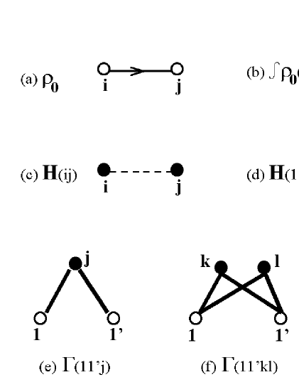
FIG. 1.: The various diagrams corresponding to the terms in Eq. (61)

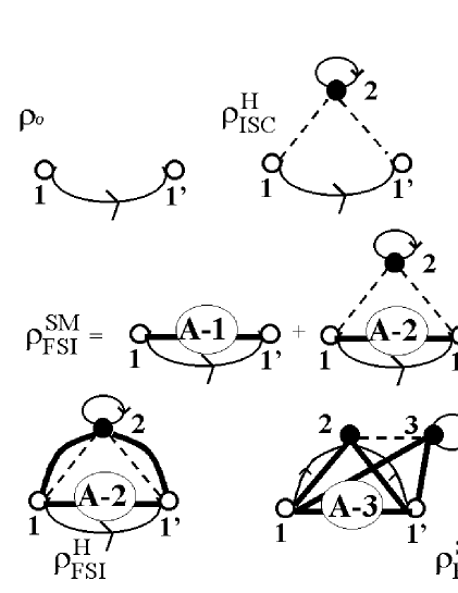
FIG. 2.: The various diagrams corresponding to the terms in Eq. (42) (only the direct contributions are shown)

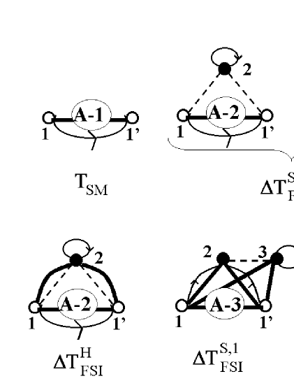
FIG. 3.: The various diagrams corresponding to the terms of the nuclear transparency, Eq. (72) (only the direct contributions are shown)

REFERENCES

• [1] S. Boffi, C. Giusti and F. D. Pacati, Phys. Rep. 226, 1 (1993)
• [2] S. J. Brodsky , in Proceedings of the 13th International Symposium on Multiparticle Dynamics, Ed. by E. W. Kittel, W. Metzger, and A. Stergiou (world Scientific, Singapore, 1982), p.964
• [3] A. Mueller, in Proceedings of the 17th Rencontre de Moriond, Ed. by J. Tranh Thanh Van (Editions Frontieres, Gif-sur-Yvette, 1982), p.13
• [4] L. L. Frankfurt, G. A. Miller and M. Strikman, Annu. Rev. Part. Sci. 45,501 (1994)
N. N. Nikolayev, Surveys in High Energy Physics 7,1 (1994)
• [5] S.C. Pieper, R.B. Wiringa and V.R. Pandharipande, Phys. Rev. C46, 141(1992).
• [6] O. Benhar et al, Phys. Rev. Lett. 69,881 (1992); Phys. Lett. B359,8 (1995)
• [7] T. S. H. Lee and G. A. Miller, Phys. Rev. C45,1863(1992)
• [8] N. N. Nikolayev et al, Phys. Lett. B317,281 (1993)
• [9] N. N. Nikolaev, J. Speth and B.G. Zakharov, J. Exp. Theor. Phys. 82, 1046 (1996)
• [10] A. Bianconi et al, Phys. Lett. 338,123 (1994).
• [11] A. Bianconi et al, Nucl. Phys. A608,437 (1996).
• [12] A. S. Rinat and B. K. Jennings, Nucl. Phys. A568,873 (1994)
A. S. Rinat and M. F. Taragin, Phys. Rev. C52,28 (1995)
• [13] L. L. Frankfurt, E. J. Moniz, M. M. Sargsyan and M. I. Strikman, Phys. Rev. C51, 3435 (1995)
• [14] A. Kohama, K. Yazaki and R. Seki, Nucl. Phys. A551,687 (1993)
R. Seki et al, Phys.Lett. B383,133 (1996)
• [15] M. Gaudin, J. Gillespie and G. Ripka, Nucl. Phys. A176,237 (1971)
• [16] O. Bohigas and S. Stringari, Phys. Lett. B95,9 (1980)
M. F. Flynn et al Nucl. Phys. A427,253 (1984)
• [17] O. Benhar, C. Ciofi degli Atti, S. Liuti and G. Salme, Phys. Lett. 28, 885 (1986)
• [18] F. Arias de Saavedra, G. Co’ and M. M. Renis Phys. Rev.55, 673 (1997)
• [19] C. Ciofi degli Atti, H. Morita and D. Treleani, to appear, and nucl-th/9901086
• [20] I.E. Lagaris and V.R. Pandharipande, Nucl. Phys. A359, 331 (1981); O. Benhar et al, Phys. Lett. B359,8 (1995)
• [21] H. Morita, C. Ciofi degli Atti, and D. Treleani, to appear
• [22] L. L. Foldy and J. D. Walecka, Ann. Phys. (NY) 54, 447 (1969).