The Nuclear Physics of Solar and Supernova Neutrino Detection

Abstract

This talk provides a basic introduction for students interested in the responses of detectors to solar, supernova, and other low-energy neutrino sources. Some of this nuclear physics is then applied in a discussion of nucleosynthesis within a Type II supernova, including the r-process and the $\nu$-process.

1. Introduction

It is a pleasure to have this opportunity to visit Tokyo Metropolitan University and address this group of students and researchers interested in neutrino physics. Professor Minakata has asked me to provide a pedagogical overview of the nuclear physics governing the detection of solar, supernova, and other low-energy neutrinos. As the following presentation is very elementary, I apologize to those of you who are already familiar with the subject.

The talk begins with a discussion of the allowed and first-forbidden responses of nuclei to low-energy neutrinos. To illustrate how the allowed response can be crucial to efforts to detect solar neutrinos, I discuss the classic example of the ³⁷Cl experiment. Similarly, first-forbidden responses are generally quite important to the interaction of heavy-flavor neutrinos from core-collapse supernovae. I discuss some examples from explosive nucleosynthesis – the r-process and the $\nu$-process – to illustrate some of the issues.

2. The allowed response

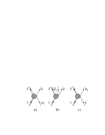
Figure 1 shows several semileptonic weak interactions that take place between nucleons or in nuclei [19]. Among such reactions important to astrophysics, two of the most familiar are the decay of the free neutron

$$n\rightarrow p+e^{-}+\bar{\nu}_{e},$$

a reaction that influences the n/p ratio in big-bang nucleosynthesis, and the driving reaction of the solar $pp$ chain

$$p+p\rightarrow d+e^{+}+\nu_{e}.$$

The latter can be thought of as the decay of a free proton in the plasma, made possible energetically by the proximity of a second proton, within the range of the nuclear force (several fermis), so that the final n+p state can form a bound deuteron. It is the binding energy of the deuteron that allows the reaction to take place.

Fig. 1.: Semileptonic weak interactions of interest: a) charged current neutrino reaction (e.g., ³⁷Cl($\nu,e^{-})^{37}$Ar); b) $\beta^{-}$ decay; and c) electron capture (e.g., ³⁷Ar(EC)³⁷Cl).

As preparation for our discussion of nuclei, first consider the rate for neutron $\beta$ decay

$$d\omega=|M|^{2}{d^{3}p_{p}\over(2\pi)^{3}}{M_{p}\over E_{p}}{d^{3}p_{e}\over(2\pi)^{3}}{m_{e}\over E_{e}}{d^{3}p_{\nu}\over(2\pi)^{3}}{m_{\nu}\over E_{\nu}}(2\pi)^{4}\delta^{4}(p_{n}-p_{p}-p_{e}-p_{\nu}).$$ (1)

(Note that I use a spinor normalization convention where all fermions are treated as massive, including neutrinos.) The invariant amplitude $M$ is taken to be a contact current-current interaction, because the momentum transfered between the leptons and nucleon is so much smaller than the mass of the W boson. Thus

$$M=\cos\theta_{c}{G_{F}\over\sqrt{2}}\bar{u}(p)\gamma^{\mu}(1-g_{A}\gamma_{5})u(n)\bar{u}(e)\gamma_{\mu}(1-\gamma_{5})v(\nu)$$ (2)

where $G_{F}$ is the weak coupling constant measured in muon decay and $\cos\theta_{c}$ gives the amplitude for the weak interaction to connect the u quark to its first-generation partner, the d quark. The origin of this effective amplitude is the underlying standard model predictions for the elementary quark and lepton currents. The weak interactions at this level are predicted by the standard model to be exactly left handed. Experiment shows that the effective coupling of the W boson to the nucleon is governed by

$$(1-g_{A}\gamma_{5})$$

where $g_{A}\sim 1.26$. The axial coupling is thus shifted from its underlying value by the strong interactions responsible for the binding of the quarks within the nucleon.

The extension to nuclear systems traditionally begins with the observation that nucleons in the nucleus are rather nonrelativistic, $v/c\sim 0.1$. The $\beta$ decay amplitude $\bar{u}(p)\gamma^{\mu}(1-g_{A}\gamma_{5})u(n)$ can be expanded in powers of $p/M$. The leading vector and axial operators are readily found to be

$$\begin{array}[]{ccc}&\underline{\gamma_{\mu}}&\underline{\gamma_{\mu}\gamma_{5}}\\ \mu=0&1&{\vec{\sigma}\cdot\vec{p}\over M}\sim{v\over c}\\ \mu=1,2,3&{\vec{p}\over M}\sim{v\over c}&\vec{\sigma}\end{array}$$

Thus it is the time-like part of the vector current and the space-like part of the axial-vector current that survive in the nonrelativistic limit.

(In a nucleus these currents must be corrected for the presence of meson exchange contributions. The corrections to the vector charge and axial three-current, which we just pointed out survive in the nonrelativistic limit, are of order $(v/c)^{2}\sim$ 1%. Thus the naive one-body currents are a very good approximation to the nuclear currents. In contrast, exchange current corrections to the axial charge and vector three-current operators are of order $v/c$, and thus of relative order 1. This difficulty for the vector three-current can be largely circumvented, because current conservation as embodied in the generalized Siegert’s theorem allows one to rewrite important parts of this operator in terms of the vector charge operator. In the long-wavelength limit appropriate to $\beta$ decay, all terms unconstrained by current conservation do not survive. In effect, one has replaced a current operator with large two-body corrections by a charge operator with only small corrections. In contrast, the axial charge operator is significantly altered by exchange currents even for long-wavelength processes like $\beta$ decay. Typical axial-charge $\beta$ decay rates are enhanced by $\sim$ 2 because of exchange currents.)

If such a nonrelativistic reduction is done for our nucleon $\beta$ decay amplitude, one obtains

$$M\sim\cos\theta_{c}{G_{F}\over\sqrt{2}}\left(\phi^{\dagger}(p)\phi(n)\bar{u}(e)\gamma^{0}(1-\gamma_{5})v(\nu)-\phi^{\dagger}(p)g_{A}\vec{\sigma}\phi(n)\cdot\bar{u}(e)\vec{\gamma}(1-\gamma_{5})v(\nu)\right)$$ (3)

where the $\phi$ are now two-component Pauli spinors for the nucleons. The above result is written for the $\beta$ decay $n\rightarrow p$. It is convenient to generalize it for $p\leftrightarrow n$ by introducing the isospin operators $\tau_{\pm}$ where $\tau_{+}$ $\mid$ n$\rangle$ = $\mid$ p$\rangle$ and $\tau_{-}$$\mid$ p$\rangle$ = $\mid$ n$\rangle$, with all other matrix elements being zero: the free proton does not $\beta$ decay, of course, but this is good preparation for the generalization to nuclei. Finally, we square the invariant amplitude, integrate over the outgoing electron, neutrino, and final nucleon three-momenta, average over initial nucleon spin, and sum over final nucleon spin, electron spin, and neutrino spin. The result is

$$\omega=G_{F}^{2}\cos^{2}\theta_{c}{1\over 2\pi^{3}}\int_{m_{e}}^{w}(w-\epsilon)^{2}\epsilon\sqrt{\epsilon^{2}-m_{e}^{2}}d\epsilon{1\over 2}\left(|\langle f||\tau_{\pm}||i\rangle|^{2}+g_{A}^{2}|\langle f||\sigma\tau_{\pm}||i\rangle|^{2}\right)$$ (4)

where $f$ and $i$ are the final and initial nucleon states, $w$ is the energy release in the decay, and $\epsilon$ is the electron energy. The $\tau_{+}$ operator corresponds to $\beta^{-}$ decay and the $\tau_{-}$ to $\beta^{+}$ decay. The notation $||$ denotes a matrix element reduced in angular momentum. One immediately sees, for large energy release $w$, that rates scale as $w^{5}$.

This result easily generalizes to nuclear decay. Given our comments about exchange currents, the first step is the replacement

$$\tau_{\pm}\rightarrow\sum_{i=1}^{A}\tau_{\pm}(i)$$

$$\sigma\tau_{\pm}\rightarrow\sum_{i=1}^{A}\sigma(i)\tau_{\pm}(i).$$

We also have to worry about an approximation in our nucleon $\beta$ decay discussion, the treatment of the nucleon as an elementary, structureless particle. This is certainly appropriate for momentum scales below the inverse size of the nucleon, as the nucleon’s structure then cannot be resolved, and for energy transfers small compared to nucleon excitation energies. Both conditions are easily satisfied in neutron $\beta$ decay. In nuclear $\beta$ decay the issue is not so clear, especially as decays can often populate a collection of states in the daughter nucleus. If the lepton states are treated as plane waves, the operators further generalize to

$$\sum_{i=1}^{A}e^{i\vec{k}\cdot\vec{r}(i)}\tau_{\pm}(i)$$

$$\sum_{i=1}^{A}e^{i\vec{k}\cdot\vec{r}(i)}\sigma(i)\tau_{\pm}(i)$$

where $\vec{r}(i)$ is the coordinate of the $ith$ nucleon relative to the nuclear center of mass. (The center-of-mass coordinate would be integrated out to give the overall three-momentum conservation for the $\beta$ decay.) In $\beta$ decay and in solar neutrino reactions, the three-momentum transfer to the nucleus $|\vec{k}|$ is much smaller than the typical inverse nuclear size, $\sim 160/A^{1/3}$ MeV. Thus as long as one is interested in transitions where the operators $\tau$ or $\sigma\tau$ connect the initial and final states of interest, the effects of the momentum transfer can be ignored. Of course, if this is not the case, then the transition amplitude is nonzero only because of the finite momentum transfer. If one expands the plane wave in powers of $\vec{k}\cdot\vec{r}(i)$, then a transition has a degree of “forbiddenness” according to the number of powers required to produce a nonzero amplitude.

For the moment we will restrict ourselves to allowed transitions where the effects of the momentum transfer can be ignored. The nuclear decay rate is then obtained by substituting into the neutron result

$${1\over 2J_{i}+1}(|\langle f||\sum_{i=1}^{A}\tau_{\pm}(i)||i\rangle|^{2}+g_{A}^{2}|\langle f||\sum_{i=1}^{A}\sigma(i)\tau_{\pm}(i)||i\rangle|^{2}).$$ (5)

The factor $1/(2J_{i}+1)$ replacing the 1/2 in the neutron result comes from the average over initial nuclear spin directions. As the nuclear Coulomb field can significantly distort the wave function of the outgoing electron or positron, a final step is to correct the lepton phase space by

$$F(Z,\epsilon)=|F_{0}(Z,\epsilon)|^{2}={2\pi\eta\over e^{2\pi\eta}-1}~{}~{}\mathrm{where}~{}~{}\eta={Z_{f}Z_{e}\alpha\over\beta}$$

where $\beta$ is the electron/positron velocity and $F_{0}(Z,\epsilon)$ is the s-wave Coulomb wave function in the field of the daughter nucleus of charge $Z_{f}$, evaluated at the nuclear origin. (This is a reasonable approximation for small $Z_{f}$; for heavier nuclei, however, the usual procedure is to solve the Dirac equation for an extensive nuclear charge, evaluating the resulting wave function at the nuclear surface.)

The spin-independent and spin-dependent operators appearing above are known as the Fermi and Gamow-Teller operators. The Fermi operator is proportional to the isospin raising/lowering operator: in the limit of good isopsin, which typically is good to 5% or better in the description of low-lying nuclear states, it can only connect states in the same isospin multiplet, that is, states with a common spin-spatial structure. If the initial state has isospin $(T_{i},M_{Ti})$, this final state has $(T_{i},M_{Ti}\pm 1)$ for $\beta^{-}$ and $\beta^{+}$ decay, respectively, and is called the isospin analog state (IAS). In the limit of good isospin the sum rule for this operator in then particularly simple

$$\sum_{f}{1\over 2J_{i}+1}|\langle f||\sum_{i=1}^{A}\tau_{+}(i)||i\rangle|^{2}={1\over 2J_{i}+1}|\langle IAS||\sum_{i=1}^{A}\tau_{+}(i)||i\rangle|^{2}=|N-Z|.$$ (6)

The excitation energy of the IAS relative to the parent ground state can be estimated accurately from the Coulomb energy difference [9]

$$E_{IAS}\sim({1.728Z\over 1.12A^{1/3}+0.78}-1.293)\mathrm{MeV}.$$ (7)

The angular distribution of the outgoing electron for a pure Fermi $(N,Z)+\nu\rightarrow(N-1,Z+1)+e^{-}$ transition is 1 + $\beta\cos\theta_{\nu e}$, and thus forward peaked. Here $\beta$ is the electron velocity.

The Gamow-Teller (GT) response is more complicated, as the operator can connect the ground state to many states in the final nucleus. In general we do not have a precise probe of the nuclear GT response apart from weak interactions themselves. However a good approximate probe is provided by forward-angle (p,n) scattering off nuclei, a technique that has been developed in particular by experimentalists at the Indiana University Cyclotron Facility. The (p,n) reaction transfers isospin and thus is superficially like $(\nu,e^{-})$. At forward angles (p,n) reactions involve negligible three-momentum transfers to the nucleus. Thus the nucleus should not be radially excited. It thus seems quite plausible that forward-angle (p,n) reactions probe the isospin and spin of the nucleus, the macroscopic quantum numbers, and thus the Fermi and GT responses. For typical transitions, the correspondence between (p,n) and the weak GT operators is believed to be accurate to about 10%. Of course, in a specific transition, much larger discrepancies can arise.

The (p,n) studies demonstrate that the GT strength tends to concentrate in a broad resonance centered at a position $\delta=E_{GT}-E_{IAS}$ relative to the IAS given by [14]

$$\delta\sim(7.0-28.9{N-Z\over A})~{}\mathrm{MeV}.$$ (8)

Thus while the peak of the GT resonance is substantially above the IAS for $N\sim Z$ nuclei, it drops with increasing neutron excess. Thus $\delta\sim 0$ for Pb. A typical value for the full width at half maximum $\Gamma$ is $\sim$ 5 MeV.

The approximate Ikeda sum rule constrains the difference in the $\beta^{-}$ and $\beta^{+}$ strengths

$$\sum_{f}(|M_{GT}^{fi}(\beta^{-})|^{2}-|M_{GT}^{fi}(\beta^{+})|^{2})=3(N-Z)$$ (9)

where

$$|M_{GT}^{fi}(\beta^{-})|^{2}={1\over 2J_{i}+1}|\langle f||\sum_{i=1}^{A}\sigma(i)\tau_{+}(i)||i\rangle|^{2}.$$ (10)

In many cases of interest in heavy nuclei, the strength in the $\beta^{+}$ direction is largely blocked. For example, in a naive $2s1d$ shell model description of ³⁷Cl, discussed below, the p $\rightarrow$ n direction is blocked by the closed neutron shell at N=20. Thus this relation can provide an estimate of the total $\beta^{-}$ strength. Experiment shows that the $\beta^{-}$ strength found in and below the GT resonance does not saturate the Ikeda sum rule, typically accounting for $\sim(60-70)$ % of the total. Measured and shell model predictions of individual GT transition strengths tend to differ systematically by about the same factor. Presumably the missing strength is spread over a broad interval of energies above the GT resonance. This is not unexpected if one keeps in mind that the shell model is an approximate effective theory designed to describe the long wavelength modes of nuclei: such a model should require effective operators, renormalized from their bare values. Phenomenologically, the shell model seems to require $g_{A}^{eff}\sim$ 1.0 as well as a small spin-tensor term $(\sigma\otimes Y_{2}(\hat{r}))_{J=1}$ of relative strength $\sim$ 0.1 [2].

The angular distribution of GT $(N,Z)+\nu_{e}\rightarrow(N-1,Z+1)+e^{-}$ reactions is $3-\beta\cos\theta_{\nu e}$, corresponding to a gentle peaking in the backward direction.

The above discussion of allowed responses can be repeated for neutral current processes such as $(\nu,\nu^{\prime})$. The analog of the Fermi operator contributes only to elastic processes, where the standard model nuclear weak charge is approximately the neutron number. As this operator does not generate transitions, it is not yet of much interest for solar or supernova neutrino detection, though there are efforts to develop low-threshold detectors (e.g., cryogenic technologies) where the modest recoil nuclear energies might be detectable. The analog of the GT response involves

$$|M_{GT}^{fi}(\nu,\nu^{\prime})|^{2}={1\over 2J_{i}+1}|\langle f||\sum_{i=1}^{A}\sigma(i){\tau_{3}(i)\over 2}||i\rangle|^{2}.$$ (11)

The operator appearing in this expression is familiar from magnetic moments and magnetic transitions, where the large isovector magnetic moment ($\mu_{v}\sim$ 4.706) often leads to it dominating the orbital and isoscalar spin operators.

3. The Response of the ³⁷Cl Detector

An interesting example of these issues in the context of a practical detector is provided by the ³⁷Cl solar neutrino experiment of Davis and his collaborators. Davis succeeded in recovering and counting the few atoms of ³⁷Ar produced by solar neutrinos in a 0.615 kiloton C₂Cl₄ detector via the reaction ³⁷Cl($\nu,e^{-})^{37}$Ar. The capture rate determined from three decades of measurements in 2.56 $\pm$ 0.16 $\pm$ 0.16 SNU [7] (1 SNU = 10^-36 captures/target atom/s), or about 1/3 that predicted by the standard solar model, conventional particle physics, and the accepted value for the ³⁷Cl neutrino capture cross section. This experiment was the first manifestation of the solar neutrino problem and remains crucial to current conclusions that neutrino oscillations may be responsible for the neutrino deficit.

The strong conclusions drawn from the ³⁷Cl experiment depend on an accurately determined neutrino capture cross section. Because the threshold for ³⁷Cl$(\nu,e^{-})^{37}$Ar (0.814 MeV) is well above the pp neutrino endpoint, the important neutrino sources are from the ⁷Be and ⁸B solar reactions. The ⁷Be neutrinos can only excite the transition to the ground state of ³⁷Ar, which is relatively weak (log$ft$ = 5.10). Thus the capture rate should be dominated by the high energy ⁸B neutrinos (endpoint $\sim$ 15 MeV).

The nuclear (not atomic) mass difference between ³⁷Cl and ³⁷Ar is 0.303 MeV. The Coulomb energy difference formula (Eq. 7) for the position of the IAS gives

$$E_{IAS}\sim 5.22\mathrm{MeV}.$$

So we conclude that the analog state should reside at $\sim$ 4.92 MeV in ³⁷Ar. Experiment has identified the IAS at 4.99 MeV. In the limit of good isospin the superallowed (Fermi) transition to the IAS has $|M_{F}|^{2}$ = N - Z = 3.0; this transition accounts for about 70% of the ⁸B capture rate.

Now the interesting issue is the model-dependent GT response. While we have noted that the total GT response is about three times the Fermi response (taking $g_{A}^{eff}\sim$ 1), its contribution to the capture rate depends on its distribution, particularly at low excitation energies where the ⁸B neutrino cross section phase space is large. As the effective particle breakup threshold for ³⁷Ar is 8.79 MeV, GT transitions to states above this energy clearly do not contribute. According to our estimate (see Eq. (8)) for $\delta=E_{GT}-E_{IAS}\sim 4.66$ MeV, the peak of the GT distribution should be at an excitation energy $\sim$ 9.6 MeV, relative to the ground state of ³⁷Ar. The two strongest peaks in the forward-angle (p,n) studies are in the region between 7 and 10 MeV, roughly in accord with expectations. Thus much of the GT strength is in the continuum, and still more resides above the IAS, where the neutrino phase space drops rapidly with increasing excitation energy.

To put the capture cross section on firm ground, a reliable map of the strength and distribution of the GT bound state response is needed. In 1964 Bahcall and Barnes [4] pointed out that the needed information could be obtained from the delayed proton spectrum following the $\beta$ decay of ³⁷Ca, as illustrated in Fig. 2. Assuming isospin invariance, the decay ³⁷Ca($\beta^{+})^{37}$K is the mirror reaction to ³⁷Cl($\nu,e^{-})^{37}$Ar. As the ³⁷K levels above the first excited state are unstable to proton emission, the allowed matrix elements for these levels can be deduced from the spectrum and intensities of the delayed protons. The transition to the ground state of ³⁷Ar is known directly, as this transition determines the electron capture lifetime of ³⁷Ar. The final needed constraint on the transition to the first excited state is imposed by the total rate for ³⁷Ca $\beta$ decay. Thus, to the extent that isospin invariance relates the mirror systems accurately, the needed GT strengths can be taken entirely from experiment.

Fig. 2.: Decay schemes of A=37 nuclei. For simplicity only the lowest T = 1/2 and T = 3/2 levels are shown. The important particle decay thresholds for states in ³⁷Ar and ³⁷K are indicated. Atomic masses in MeV are indicated by [0.00], etc. All other energies are excitation energies in the indicated nuclei.

The ³⁷Ca($\beta^{+})^{37}$K delayed proton spectrum was measured [16]] by two groups; the deduced $ft$ values were the basis for the ³⁷Cl cross section used for 20 years. Interestingly these early experiments were flawed because of a simplifying assumption, that the delayed protons from ³⁷K were accompanied by production of the daughter nucleus ³⁶Ar in its ground state. In 1987 Adelberger and Haxton [1], noticing that the GT distribution deduced from the delayed proton experiments differed significantly from that recently measured [17] in ³⁷Cl(p,n), argued that the likely source of this discrepancy was the population of ³⁶Ar in its 2⁺ first excited state (1.97 MeV) in the delayed proton experiments. The states populated in ³⁷K by allowed $\beta$ decay have the spins and parity 1/2⁺, 3/2⁺, and 5/2⁺. Thus the reason that the ³⁶Ar first excited state should be important is clear: the 3/2⁺ and 5/2⁺ states can populate the 2⁺ state by s-wave proton emission, while the ground state requires d-wave emission.

The conclusion was that the ³⁷Ca experiment had to be redone in a kinematically complete way, where 1.97 MeV $\gamma$s accompanying the decay of the 2⁺ state could be observed in coincidence with the delayed protons. A series of elegant experiments were conducted by Garcia et al.[10], resulting in the determination $\sigma(^{8}$B) = 1.09 $\pm$ 0.09. Interestingly, this value was little changed from that used previously: ignoring the population of the 2⁺ state produced two largely compensating errors. The affected transitions were placed too low in energy (by 1.97 MeV), but their strengths were also underestimated as the wrong ³⁷Ca $\beta$ decay phase space was then employed. However, the sizeable discrepancies between the ³⁷Ca $\beta$ decay and (p,n) mappings were largely resolved, thus restoring confidence that the capture rate uncertainties in the Davis experiment were under control.

The reason for the discussions of this section is to illustrate that a reliable cross section for the ³⁷Cl experiment was obtained only after complementary calibration techniques were proposed, developed, and cross checked. This careful nuclear physics is a cornerstone of today’s arguments that the solar neutrino puzzle is likely due to new neutrino phenomena.

4. Supernovae and Supernova Neutrinos

Consider a massive star, in excess of 10 solar masses, burning the hydrogen in its core under the conditions of hydrostatic equilibrium. When the hydrogen is exhausted, the core contracts until the density and temperature are reached where 3$\alpha\rightarrow^{12}$C can take place. The He is then burned to exhaustion. This pattern (fuel exhaustion, contraction, and ignition of the ashes of the previous burning cycle) repeats several times, leading finally to the explosive burning of ²⁸Si to Fe. For a heavy star, the evolution is rapid: the star has to work harder to maintain itself against its own gravity, and therefore consumes its fuel faster. A 25 solar mass star would go through all of these cycles in about 7 My, with the final explosive Si burning stage taking a few days. The result is an “onion skin” structure of the precollapse star in which the star’s history can be read by looking at the surface inward: there are concentric shells of H, ⁴He, ¹²C, ¹⁶O and ²⁰Ne, ²⁸Si, and ⁵⁶Fe at the center.

The source of energy for this evolution is nuclear binding energy. A plot of the nuclear binding energy $\delta$ as a function of nuclear mass shows that the minimum is achieved at Fe. In a scale where the ¹²C mass is picked as zero:

¹²C     $\delta$/nucleon = 0.000 MeV

¹⁶O     $\delta$/nucleon = -0.296 MeV

²⁸Si    $\delta$/nucleon = -0.768 MeV

⁴⁰Ca    $\delta$/nucleon = -0.871 MeV

⁵⁶Fe    $\delta$/nucleon = -1.082 MeV

⁷²Ge    $\delta$/nucleon = -1.008 MeV

⁹⁸Mo    $\delta$/nucleon = -0.899 Mev

Thus once the Si burns to produce Fe, there is no further source of nuclear energy adequate to support the star. So as the last remnants of nuclear burning take place, the core is largely supported by degeneracy pressure, with the energy generation rate in the core being less than the stellar luminosity. The core density is about 2 $\times 10^{9}$ g/cc and the temperature is kT $\sim$ 0.5 MeV.

Thus the collapse that begins with the end of Si burning is not halted by a new burning stage, but continues. As gravity does work on the matter, the collapse leads to a rapid heating and compression of the matter. As the nucleons in Fe are bound by about 8 MeV, sufficient heating can release $\alpha$s and a few nucleons. At the same time, the electron chemical potential is increasing. This makes electron capture on nuclei and any free protons favorable,

$$e^{-}+p\rightarrow\nu_{e}+n.$$

Note that the chemical equilibrium condition is

$$\mu_{e}+\mu_{p}=\mu_{n}+\langle E_{\nu}\rangle.$$

Thus the fact that neutrinos are not trapped plus the rise in the electron Fermi surface as the density increases, lead to increased neutronization of the matter. The escaping neutrinos carry off energy and lepton number. Both the electron capture and the nuclear excitation and disassociation take energy out of the electron gas, which is the star’s only source of support. This means that the collapse is very rapid. Numerical simulations find that the iron core of the star ($\sim$ 1.2-1.5 solar mases) collapses at about 0.6 of the free fall velocity [13].

In the early stages of the infall the $\nu_{e}$s readily escape. But neutrinos are trapped when a density of $\sim$ 10¹²g/cm³ is reached. At this point the neutrinos begin to scatter off the matter through both charged current and coherent neutral current processes. The neutral current neutrino scattering off nuclei is particularly important, as the scattering cross section is off the total nuclear weak charge, which is approximately the neutron number. This process transfers very little energy because the mass energy of the nucleus is so much greater than the typical energy of the neutrinos. But momentum is exchanged. Thus the neutrino “random walks” out of the star. When the neutrino mean free path becomes sufficiently short, the “trapping time” of the neutrino begins to exceed the time scale for the collapse to be completed. This occurs at a density of about 10¹² g/cm³, or somewhat less than 1% of nuclear density. After this point, the energy released by further gravitational collapse and the star’s remaining lepton number are trapped within the star.

If we take a neutron star of 1.4 solar masses and a radius of 10 km, an estimate of its binding energy is

$${GM^{2}\over 2R}\sim 2.5\times 10^{53}\mathrm{ergs}.$$

Thus this is roughly the trapped energy that will later be radiated in neutrinos.

The trapped lepton fraction $Y_{L}$ is a crucial parameter in the explosion physics: a higher trapped $Y_{L}$ leads to a larger homologous core, a stronger shock wave, and easier passage of the shock wave through the outer core, as will be discussed below. Most of the lepton number loss of an infalling mass element occurs as it passes through a narrow range of densities just before trapping. The reasons for this are relatively simple: on dimensional grounds weak rates in a plasma go as $T^{5}$, where T is the temperature. Thus the electron capture rapidly turns on as matter falls toward the trapping radius, and lepton number loss is maximal just prior to trapping. Inelastic neutrino reactions have an important effect on these losses, as the coherent trapping cross section goes as $E_{\nu}^{2}$ and is thus least effective for the lowest energy neutrinos. As these neutrinos escape, inelastic reactions repopulate the low energy states, allowing the neutrino emission to continue.

The velocity of sound in matter rises with increasing density. The inner homologous core, with a mass $M_{HC}\sim 0.6-0.9$ solar masses, is that part of the iron core where the sound velocity exceeds the infall velocity. This allows any pressure variations that may develop in the homologous core during infall to even out before the collapse is completed. As a result, the homologous core collapses as a unit, retaining its density profile. That is, if nothing were to happen to prevent it, the homologous core would collapse to a point.

The collapse of the homologous core continues until nuclear densities are reached. As nuclear matter is rather incompressible ($\sim$ 200 MeV/f³), the nuclear equation of state is effective in halting the collapse: maximum densities of 3-4 times nuclear are reached, e.g., perhaps $6\cdot 10^{14}$ g/cm³. The innermost shell of matter reaches this supernuclear density first, rebounds, sending a pressure wave out through the homologous core. This wave travels faster than the infalling matter, as the homologous core is characterized by a sound speed in excess of the infall speed. Subsequent shells follow. The resulting series of pressure waves collect near the sonic point (the edge of the homologous core). As this point reaches nuclear density and comes to rest, a shock wave breaks out and begins its traversal of the outer core.

Initially the shock wave may carry an order of magnitude more energy than is needed to eject the mantle of the star (less than 10⁵¹ ergs). But as the shock wave travels through the outer iron core, it heats and melts the iron that crosses the shock front, at a loss of $\sim$ 8 MeV/nucleon. The enhanced electron capture that occurs off the free protons left in the wake of the shock, coupled with the sudden reduction of the neutrino opacity of the matter (recall $\sigma_{coherent}\sim N^{2}$), greatly accelerates neutrino emission. This is another energy loss. [Many numerical models predict a strong “breakout” burst of $\nu_{e}$s in the few milliseconds required for the shock wave to travel from the edge of the homologous core to the neutrinosphere at $\rho\sim 10^{12}$ g/cm³ and $r\sim 50$ km. The neutrinosphere is the term from the neutrino trapping radius, or surface of last scattering.] The summed losses from shock wave heating and neutrino emission are comparable to the initial energy carried by the shock wave. Thus most numerical models fail to produce a successful “prompt” hydrodynamic explosion.

Two explosion mechanisms were seriously considered in the last two decades. In the prompt mechanism [8] described above, the shock wave is sufficiently strong to survive the passage of the outer iron core with enough energy to blow off the mantle of the star. The most favorable results were achieved with smaller stars (less than 15 solar masses) where there is less overlying iron, and with soft equations of state, which produce a more compact neutron star and thus lead to more energy release. In part because of the lepton number loss problems discussed earlier, now it is widely believed that this mechanism fails for all but unrealistically soft nuclear equations of state.

The delayed mechanism [5] begins with a failed hydrodynamic explosion; after about 0.01 seconds the shock wave stalls at a radius of 200-300 km. It exists in a sort of equilibrium, gaining energy from matter falling across the shock front, but loosing energy to the heating of that material. However, after perhaps 0.5 seconds, the shock wave is revived due to neutrino heating of the nucleon “soup” left in the wake of the shock. This heating comes primarily from charged current reactions off the nucleons in that nucleon gas; quasielastic scattering also contributes. This high entropy radiation-dominated gas may reach two MeV in temperature. The pressure exerted by this gas helps to push the shock outward. It is important to note that there are limits to how effective this neutrino energy transfer can be: if matter is too far from the core, the coupling to neutrinos is too weak to deposite significant energy. If too close, the matter may be at a temperature (or soon reach a temperature) where neutrino emission cools the matter as fast or faster than neutrino absorption heats it. The term “gain radius” is used to describe the region where useful heating is done.

This subject is still controversial and unclear. The problem is numerically challenging, forcing modelers to handle the difficult hydrodynamics of a shock wave; the complications of the nuclear equation of state at densities not yet accessible to experiment; modeling in two or three dimensions; handling the slow diffusion of neutrinos; etc. Not all of these aspects can be handled reasonably at the same time, even with existing supercomputers. Thus there is considerable disagreement about whether we have any supernova model that succeeds in ejecting the mantle.

However the explosion proceeds, there is agreement that 99% of the 3 $\cdot 10^{53}$ ergs released in the collapse is radiated in neutrinos of all flavors. The time scale over which the trapped neutrinos leak out of the protoneutron star is about 3 seconds. (Fits to SN1987A give, assuming an exponential cooling $e^{-t/\tau}$, $\tau\sim$ 4.5 s [3]) Through most of their migration out of the protoneutron star, the neutrinos are in flavor equilibrium

$$\mathrm{e.g.},~{}~{}\nu_{e}+\bar{\nu}_{e}\leftrightarrow\nu_{\mu}+\bar{\nu}_{\mu}.$$

As a result, there is an approximate equipartition of energy among the neutrino flavors. After weak decoupling, the $\nu_{e}$s and $\bar{\nu_{e}}$s remain in equilibrium with the matter for a longer period than their heavy-flavor counterparts, due to the larger cross sections for scattering off electrons and because of the charge-current reactions

$$\nu_{e}+n\leftrightarrow p+e^{-}$$

$$\bar{\nu_{e}}+p\leftrightarrow n+e^{+}.$$

Thus the heavy flavor neutrinos decouple from deeper within the star, where temperatures are higher. Typical calculations yield

$$T_{\nu_{\mu}}\sim T_{\nu_{\tau}}\sim 8\mathrm{MeV}$$

$$T_{\nu_{e}}\sim 3.5\mathrm{MeV}~{}~{}~{}T_{\bar{\nu_{e}}}\sim 4.5\mathrm{MeV}.$$

The difference between the $\nu_{e}$ and $\bar{\nu_{e}}$ temperatures is a result of the neutron richness of the matter, which enhances the rate for charge-current reactions of the $\nu_{e}$s, thereby keeping them coupled to the matter somewhat longer.

This temperature hierarchy is crucially important to nucleosynthesis and also to possible neutrino oscillation scenarios. The three-flavor MSW level-crossing diagram is shown in Fig. 3. One very popular scenario attributes the solar neutrino problem to $\nu_{\mu}\leftrightarrow\nu_{e}$ transmutation; this means that a second crossing with a $\nu_{\tau}$ could occur at higher density. It turns out plausible seasaw mass patterns suggest a $\nu_{\tau}$ mass on the order of a few eV, which would be interesting cosmologically. The second crossing would then occur outside the neutrino sphere, that is, after the neutrinos have decoupled and have fixed spectra with the temperatures given above. Thus a $\nu_{e}\leftrightarrow\nu_{\tau}$ oscillation would produce a distinctive $T\sim 8$ MeV spectrum of $\nu_{e}$s. This has dramatic consequences for terrestrial detection and for nucleosynthesis in the supernova.

Fig. 3.: Three-flavor neutrino level-crossing diagram. One popular scenario associates the solar neutrino problem with $\nu_{e}\leftrightarrow\nu_{\mu}$ oscillations and predicts a cosmologically interested massive $\nu_{\tau}$ with $\nu_{e}\leftrightarrow\nu_{\tau}$ oscillations near the supernova neutrinosphere.

5. First Forbidden Responses and the Neutrino Process

Core-collapse supernovae are one of the major engines driving galactic chemical evolution, producing and ejecting the metals that enrich our galaxy. The discussion of the previous section described the hydrostatic evolution of a presupernova star in which large quantities of the most abundant metals (C, O, Ne, …) are synthesized and later ejected during the explosion. During the passage of the shock wave through the star’s mantle, temperature of $\sim(1-3)\cdot 10^{9}$K and are reached in the silicon, oxygen, and neon shells. This shock wave heating induces $(\gamma,\alpha)\leftrightarrow(\alpha,\gamma)$ and related reactions that generate a mass flow toward highly bound nuclei, resulting in the synthesis of iron peak elements as well as less abundant odd-A species. Rapid neutron-induced reactions are thought to take place in the high-entropy atmosphere just above the mass cut, producing about half of the heavy elements above A $\sim$ 80. This is the subject of the next section. Finally, the $\nu$-process described below is responsible for the synthesis of rare species such as ¹¹B and ¹⁹F. This process involves the response of nuclei at momentum transfers where the allowed approximation is no longer valid. Thus we will use the $\nu$-process in this section to illustrate some of the relevant nuclear physics.

One of the problems – still controversial – that may be connected with the neutrino process is the origin of the light elements Be, B and Li, elements which are not produced in sufficient amounts in the big bang or in any of the stellar mechanisms we have discussed. The traditional explanation has been cosmic ray spallation interactions with C, O, and N in the interstellar medium. In this picture, cosmic ray protons collide with C at relatively high energy, knocking the nucleus apart. So in the debris one can find nuclei like ¹⁰B, ¹¹B, and ⁷Li.

But there are some problems with this picture. First of all, this is an example of a secondary mechanism: the interstellar medium must be enriched in the C, O, and N to provide the targets for these reactions. Thus cosmic ray spallation must become more effective as the galaxy ages. The abundance of boron, for example, would tend to grow quadratically with metalicity, since the rate of production goes linearly with metalicity. But observations, especially recent measurements with the Hubble Space Telescope (HST), find a linear growth in the boron abundance [18].

A second problem is that the spectrum of cosmic ray protons peaks near 1 GeV, leading to roughly comparable production of the two isotopes ¹⁰B and ¹¹B. That is, while it takes more energy to knock two nucleons out of carbon than one, this difference is not significant compared to typical cosmic ray energies. More careful studies lead to the expectation that the abundance ratio of ¹¹B to ¹⁰B might be $\sim$ 2. In nature, it is greater than 4.

Fans of cosmic ray spallation have offered solutions to these problems, e.g., similar reactions occurring in the atmospheres of nebulae involving lower energy cosmic rays. As this suggestion was originally stimulated by the observation of nuclear $\gamma$ rays from Orion, now retracted, some of the motivation for this scenario has evaporated. Here I focus on an alternative explanation, synthesis via neutrino spallation.

Previously we spoke about weak interactions in nuclei involving the Gamow-Teller (spin-flip) and Fermi operators. These are the appropriate operators when one probes the nucleus at a wavelength – that is, at a size scale – where the nucleus responds like an elementary particle. We can then characterize its response by its macroscopic quantum numbers, the spin and charge. On the other hand, the nucleus is a composite object and, therefore, if it is probed at shorter length scales, all kinds of interesting radial excitations will result, analogous to the vibrations of a drumhead. For a reaction like neutrino scattering off a nucleus, the full operator involves the additional factor

$$e^{i\vec{k}\cdot\vec{r}}\sim 1+i\vec{k}\cdot\vec{r}$$

where the expression on the right is valid if the magnitude of $\vec{k}$ is not too large. Thus the full charge operator includes a “first forbidden” term

$$\sum_{i=1}^{A}\vec{r}_{i}\tau_{3}(i)$$

and similarly for the spin operator

$$\sum_{i=1}^{A}[\vec{r}_{i}\otimes\vec{\sigma}(i)]_{J=0,1,2}\tau_{3}(i).$$

These operators generate collective radial excitations, leading to the so-called “giant resonance” excitations in nuclei. The giant resonances are typically at an excitation energy of 20-25 MeV in light nuclei. One important property is that these operators satisfy a sum rule (Thomas-Reiche-Kuhn) of the form

$$\sum_{f}|\langle f|\sum_{i=1}^{A}r(i)\tau_{3}(i)|i\rangle|^{2}\sim{NZ\over A}\sim{A\over 4}$$

where the sum extends over a complete set of final nuclear states. These first-forbidden operators tend to dominate the cross sections for scattering the high energy supernova neutrinos ($\nu_{\mu}$s and $\nu_{\tau}$s), with $E_{\nu}\sim$ 25 MeV, off light nuclei. From the sum rule above, it follows that nuclear cross sections per target nucleon are roughly constant.

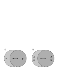
The E1 giant dipole mode described above is depicted qualitatively in Fig. 4a. This description, which corresponds to an early model of the giant resonance response by Goldhaber and Teller [11], involves the harmonic oscillation of the proton and neutron fluids against one another. The restoring force for small displacements would be linear in the displacement and dependent on the nuclear symmetry energy. There is a natural extension of this model to weak interactions, where axial excitations occur. For example, one can envision a mode similar to that of Fig. 4a where the spin-up neutrons and spin-down protons oscillate against spin-down neutrons and spin-up protons, the spin-isospin mode of Fig. 4b. This mode is one that arises in a simple SU(4) extension of the Goldhaber-Teller model, derived by assuming that the nuclear force is spin and isospin independent, at the same excitation energy as the E1 mode. In full, the Goldhaber-Teller model predicts a degenerate 15-dimensional supermultiplet of giant resonances, each obeying sum rules analogous to the TRK sum rule. While more sophisticated descriptions of the giant resonance region are available, of course, this crude picture is qualitatively accurate.

Fig. 4.: Schematic illustration of a) the E1 giant dipole mode familiar from electromagnetic interactions and b) a spin-isospin giant dipole mode associated with the first-forbidden weak axial response.

This nuclear physics is important to the $\nu$-process [21]. The simplest example of $\nu$-process nucleosynthesis involves the Ne shell in a supernova. Because of the first-forbidden contributions, the cross section for inelastic neutrino scattering to the giant resonances in Ne is $\sim 3\cdot 10^{-41}$ cm²/flavor for the more energetic heavy-flavor neutrinos. This reaction

$$\nu+A\rightarrow\nu^{\prime}+A^{*}$$

transfers an energy typical of giant resonances, $\sim$ 20 MeV. A supernova releases about 3 $\times 10^{53}$ ergs in neutrinos, which converts to about $4\times 10^{57}$ heavy flavor neutrinos. The Ne shell in a 20 M_⊙ star has at a radius $\sim$ 20,000 km. Thus the neutrino fluence through the Ne shell is

$$\phi\sim{4\cdot 10^{57}\over 4\pi(20,000\mathrm{km})^{2}}\sim 10^{38}/\mathrm{cm}^{2}.$$

Thus folding the fluence and cross section, one concludes that approximately 1/300th of the Ne nuclei interact.

This is quite interesting since the astrophysical origin of ¹⁹F had not been understood. The only stable isotope of fluorine, ¹⁹F has an abundance

$${{}^{19}\mathrm{F}\over{}^{20}\mathrm{Ne}}\sim{1\over 3100}.$$

This leads to the conclusion that the fluorine found in toothpaste was created by neutral current neutrino reactions deep inside some ancient supernova.

The calculation [21] of the final ¹⁹F/²⁰Ne ratio is more complicated than the simple 1/300 ratio given above:
$\bullet$ When Ne is excited by $\sim$ 20 MeV through inelastic neutrino scattering, it breaks up in two ways

$${}^{20}\mathrm{Ne}(\nu,\nu^{\prime})^{20}\mathrm{Ne}^{*}\rightarrow^{19}\mathrm{Ne}+n\rightarrow^{19}\mathrm{F}+e^{+}+\nu_{e}+n$$

$${}^{20}\mathrm{Ne}(\nu,\nu^{\prime})^{20}\mathrm{Ne}^{*}\rightarrow^{19}\mathrm{F}+p$$

with the first reaction occurring half as frequently as the second. As both channels lead to ¹⁹F, we have correctly estimated the instantaneous abundance ratio in the Ne shell of

$${{}^{19}\mathrm{F}\over{}^{20}\mathrm{Ne}}\sim{1\over 300}.$$

$\bullet$ We must also address the issue of whether the produced ¹⁹F survives. In the first 10^-8 sec the coproduced neutrons in the first reaction react via

$${}^{15}\mathrm{O}(n,p)^{15}\mathrm{N}~{}~{}^{19}\mathrm{Ne}(n,\alpha)^{16}\mathrm{O}~{}~{}^{20}\mathrm{Ne}(n,\gamma)^{21}\mathrm{Ne}~{}~{}^{19}\mathrm{Ne}(n,p)^{19}\mathrm{F}$$

with the result that about 70% of the ¹⁹F produced via spallation of neutrons is then immediate destroyed, primarily by the $(n,\alpha)$ reaction above. In the next $10^{-6}$ sec the coproduced protons are also processed

$${}^{15}\mathrm{N}(p,\alpha)^{12}\mathrm{C}~{}~{}^{19}\mathrm{F}(p,\alpha)^{16}\mathrm{O}~{}~{}^{23}\mathrm{Na}(p,\alpha)^{20}\mathrm{Ne}$$

with the latter two reactions competing as the primary proton poisons. This makes an important prediction: stars with high Na abundances should make more F, as the ²³Na acts as a proton poison to preserve the produced F.
$\bullet$ Finally, there is one other destruction mechanism, the heating associated with the passage of the shock wave. It turns out the the F produced prior to shock wave passage can survive if it is in the outside half of the Ne shell. The reaction

$${}^{19}\mathrm{F}(\gamma,\alpha)^{15}\mathrm{N}$$

destroys F for peak explosion temperatures exceeding $1.7\cdot 10^{9}$K. Such a temperature is produced at the inner edge of the Ne shell by the shock wave heating, but not at the outer edge.

If all of this physics in handled is a careful network code that includes the shock wave heating and F production both before and after shock wave passage, the following are the results:

$$\begin{array}[]{cc}\underline{[^{19}\mathrm{F}/^{20}\mathrm{Ne}]/[^{19}\mathrm{F}/^{20}\mathrm{Ne}]_{\odot}}&\underline{T_{\mathrm{heavy}~{}\nu}\mathrm{(MeV)}}\\ 0.14&4\\ 0.6&6\\ 1.2&8\\ 1.1&10\\ 1.1&12\end{array}$$

One sees that the attribution of F to the neutrino process argues that the heavy flavor $\nu$ temperature must be greater than 6 MeV, a result theory favors. One also sees that F cannot be overproduced by this mechanism: although the instantaneous production of F continues to grow rapidly with the neutrino temperature, too much F results in its destruction through the $(p,\alpha)$ reaction, given a solar abundance of the competing proton poison ²³Na. Indeed, this illustrates an odd quirk: although in most cases the neutrino process is a primary mechanism, one needs ²³Na present to produce significant F. Thus in this case the neutrino process is a secondary mechanism.

While there are other significant neutrino process products (⁷Li, ¹³⁸La, ¹⁸⁰Ta, ¹⁵N …), the most important product is ¹¹B, produced by spallation off carbon. A calculation by Timmes et al. [18] found that the combination of the neutrino process, cosmic ray spallation and big-bang nucleosythesis together can explain the evolution of the light elements. The neutrino process, which produces a great deal of ¹¹B but relatively little ¹⁰B, combines with the cosmic ray spallation mechanism to yield the observed isotope ratio. Again, one prediction of this picture is that early stars should be ¹¹B rich, as the neutrino process is primary and operates early in our galaxy’s history; the cosmic ray production of ¹⁰B is more recent. There is hope that HST studies will soon be able to descriminate between ¹⁰B and ¹¹B: as yet this has not been done.

6. The r-process

Beyond the iron peak nuclear Coulomb barriers become so high that charged particle reactions become ineffective, leaving neutron capture as the mechanism responsible for producing the heaviest nuclei. If the neutron abundance is modest, this capture occurs in such a way that each newly synthesized nucleus has the opportunity to $\beta$ decay, if it is energetically favorable to do so. Thus weak equilibrium is maintained within the nucleus, so that synthesis is along the path of stable nuclei. This is called the s- or slow-process. However a plot of the s-process in the (N,Z) plane reveals that this path misses many stable, neutron-rich nuclei that are known to exist in nature. This suggests that another mechanism is at work, too. Furthermore, the abundance peaks found in nature near masses A $\sim$ 130 and A $\sim$ 190, which mark the closed neutron shells where neutron capture rates and $\beta$ decay rates are slower, each split into two subpeaks. One set of subpeaks corresponds to the closed-neutron-shell numbers N $\sim$ 82 and N $\sim$ 126, and is clearly associated with the s-process. The other set is shifted to smaller N, $\sim$ 76 and $\sim$ 116, respectively, and is suggestive of a much more explosive neutron capture environment where neutron capture can be rapid.

This second process is the r- or rapid-process, characterized by:
$\bullet$ The neutron capture is fast compared to $\beta$ decay rates.
$\bullet$ The equilibrium maintained within a nucleus is established by $(n,\gamma)\leftrightarrow(\gamma,n)$: neutron capture fills up the available bound levels in the nucleus until this equilibrium sets in. The new Fermi level depends on the temperature and the relative $n/\gamma$ abundance.
$\bullet$ The nucleosynthesis rate is thus controlled by the $\beta$ decay rate: each $\beta^{-}$ capture coverting n $\rightarrow$ p opens up a hole in the neutron Fermi sea, allowing another neutron to be captured.
$\bullet$ The nucleosynthesis path is along exotic, neutron-rich nuclei that would be highly unstable under normal laboratory conditions.
$\bullet$ As the nucleosynthesis rate is controlled by the $\beta$ decay, mass will build up at nuclei where the $\beta$ decay rates are slow. It follows, if the neutron flux is reasonable steady over time so that equilibrated mass flow is reached, that the resulting abundances should be inversely proportional to these $\beta$ decay rates.

Let’s first explore the $(n,\gamma)\leftrightarrow(\gamma,n)$ equilibrium condition, which requires that the rate for $(n,\gamma)$ balances that for $(\gamma,n)$ for an average nucleus. So consider the formation cross section

$$A+n\rightarrow(A+1)+\gamma$$

This is an exothermic reaction, as the neutron drops into the nuclear well. Our averaged cross section, assuming a resonant reaction (the level density is high in heavy nuclei) is (see any standard nuclear astrophysics text, such as Clayton [6])

$$\langle\sigma v\rangle_{(n,\gamma)}=\left({2\pi\over\mu kT}\right)^{3/2}{\Gamma_{n}\Gamma_{\gamma}\over\Gamma}e^{-E/KT}$$ (12)

where E $\sim$ 0 is the resonance energy, and the $\Gamma$s are the indicated partial and total widths. Thus the rate per unit volume is

$$r_{(n,\gamma)}\sim N_{n}N_{A}\left({2\pi\over\mu kT}\right)^{3/2}{\Gamma_{n}\Gamma_{\gamma}\over\Gamma}$$ (13)

where $N_{n}$ and $N_{A}$ are the neutron and nuclear number densities and $\mu$ the reduced mass. This has to be compared to the $(\gamma,n)$ rate.

The $(\gamma,n)$ reaction requires the photon number density in the gas. This is given by the Bose-Einstein distribution

$$N(\epsilon)={8\pi\over c^{3}h^{3}}{\epsilon^{2}d\epsilon\over e^{\epsilon/kT}-1}$$ (14)

The high-energy tail of the normalized distribution can thus be written

$$\sim{1\over N_{\gamma}\pi^{2}}\epsilon^{2}e^{-\epsilon/kT}d\epsilon$$

where in the last expression we have set $\hbar=c=1$.

Now we need the resonant cross section in the $(\gamma,n)$ direction. For photons the wave number is proportional to the energy, so

$$\sigma_{(\gamma,n)}={\pi\over\epsilon^{2}}{\Gamma_{\gamma}\Gamma_{n}\over(\epsilon-E_{r})^{2}+(\Gamma/2)^{2}}$$ (15)

As the velocity is c =1,

$$\langle\sigma v\rangle={1\over\pi^{2}N_{\gamma}}\int_{0}^{\infty}\epsilon^{2}e^{-\epsilon/kT}d\epsilon{\pi\over\epsilon^{2}}{\Gamma_{\gamma}\Gamma_{n}\over(\epsilon-E_{r})^{2}+(\Gamma/2)^{2}}$$ (16)

We evaluate this in the usual way for a sharp resonance, remember that the energy integral over just the denominator above (the sharply varying part) is $2\pi/\Gamma$:

$$\sim{\Gamma_{\gamma}\Gamma_{n}\over N_{\gamma}}e^{-E_{r}/kT}{2\over\Gamma}$$

So that the rate becomes

$$r_{(\gamma,n)}\sim 2N_{A+1}{\Gamma_{\gamma}\Gamma_{n}\over\Gamma}e^{-E_{r}/kT}$$ (17)

Equating the $(n,\gamma)$ and $(\gamma,n)$ rates and taking $N_{A}\sim N_{A-1}$ then yields

$$N_{n}\sim{2\over(\hbar c)^{3}}\left({\mu c^{2}kT\over 2\pi}\right)^{3/2}e^{-E_{r}/kT}$$ (18)

where the $\hbar$s and $c$s have been properly inserted to give the right dimensions. Now $E_{r}$ is esssentially the binding energy. So plugging in the conditions $N_{n}\sim 3\times 10^{23}$/cm³ and $T_{9}\sim 1$, we find that the binding energy is $\sim$ 2.4 MeV. Thus neutrons are bound by about 30 times $kT$, a value that is still small compared to a typical binding of 8 MeV for a normal nucleus. (In this calculation I calculated the neutron reduced mass assuming a nuclear target with A=150.)

The above calculation fails to count spin states for the photons and nuclei and is thus not quite correct. But it makes the essential point: the r-process involves very exotic species largely unstudied in any terrestrial laboratory. It is good to bear this in mind, as in the following section we will discuss the responses of such nuclei to neutrinos. Such responses thus depend on the ability of theory to extrapolate responses from known nuclei to those quite unfamiliar.

The path of the r-process is along neutron-rich nuclei, where the neutron Fermi sea is just $\sim$ (2-3) MeV away from the neutron drip line (where no more bound neutron levels exist). After the r-process finishes (the neutron exposure ends) the nuclei decay back to the valley of stability by $\beta$ decay. This can involve some neutron spallation ($\beta$-delayed neutrons) that shift the mass number A to a lower value. But it certainly involves conversion of neutrons into protons, and that shifts the r-process peaks at N $\sim$ 82 and 126 to a lower N, off course. This effect is clearly seen in the abundance distribution: the r-process peaks are shifted to lower N relative to the s-process peaks. This is the origin of the second set of “subpeaks” mentioned at the start of the section.

It is believed that the r-process can proceed to very heavy nuclei (A $\sim$ 270) where it is finally ended by $\beta$-delayed and n-induced fission, which feeds matter back into the process at an A $\sim$ A_max/2. Thus there may be important cycling effects in the upper half of the r-process distribution.

What is the site(s) of the r-process? This has been debated many years and still remains a controversial subject.
$\bullet$ The r-process requires exceptionally explosive conditions

$\rho$(n) $\sim 10^{20}$ cm^-3   T $\sim 10^{9}$K   t $\sim$ 1s.

$\bullet$ Both primary and secondary sites proposed. Primary sites are those not requiring preexisting metals. Secondary sites are those where the neutron capture occurs on preexisting s-process seeds.
$\bullet$ Suggested primary sites include the the neutronized atmosphere above the proto-neutron star in a Type II supernova, neutron-rich jets produced in supernova explosions or in neutron star mergers, inhomogeneous big bangs, etc.
$\bullet$ Secondary sites, where $\rho$(n) can be lower for successful synthesis, include the He and C zones in Type II supernovae, the red giant He flash, etc.

The balance of evidence favors a primary site, so one requiring no preenrichment of heavy s-process metals. Among the evidence:

1) HST studies of very-metal-poor halo stars: The most important evidence are the recent HST measurements of Sneden et al. [15] of very metal-poor stars ([Fe/H] $\sim$ -1.7 to -3.12) where an r-process distribution very much like that of our sun has been seen for Z $\,>$$\sim\,$ 56. Furthermore, in these stars the iron content is variable. This suggests that the “time resolution” inherent in these old stars is short compared to galactic mixing times (otherwise Fe would be more constant). The conclusion is that the r-process material in these stars is most likely from one or a few local supernovae. The fact that the distributions match the solar r-process (at least above charge 56) strongly suggests that there is some kind of unique site for the r-process: the solar r-process distribution did not come from averaging over many different kinds of r-process events. Clearly the fact that these old stars are enriched in r-process metals also strongly argues for a primary process: the r-process works quite well in an environment where there are few initial s-process metals.

2) There are also fairly good theoretical arguments that a primary r-process occurring in a core-collapse supernova might be viable [20]. First, galactic chemical evolution studies indicate that the growth of r-process elements in the galaxy is consistent with low-mass Type II supernovae in rate and distribution. More convincing is the fact that modelers have shown that the conditions needed for an r-process (very high neutron densities, temperatures of 1-3 billion degrees) might be realized in a supernova. The site is the last material blown off the supernova, the material just above the mass cut. When this material is blown off the star initially, it is a very hot neutron-rich, radiation-dominated gas containing neutrons and protons, but an excess of the neutrons. As it expands off the star and cools, the material first goes through a freezeout to $\alpha$ particles, a step that essentially locks up all the protons in this way. Then the $\alpha$s interact through reactions like

$$\alpha+\alpha+\alpha\rightarrow^{12}C$$

$$\alpha+\alpha+n\rightarrow^{9}Be$$

to start forming heavier nuclei. Note, unlike the big bang, that the density is high enough to allow such three-body interactions to bridge the mass gaps at A = 5,8. The $\alpha$ capture continues up to heavy nuclei, to A $\sim$ 80, in the network calculations. The result is a small number of “seed” nuclei, a large number of $\alpha$s, and excess neutrons. These neutrons preferentially capture on the heavy seeds to produce an r-process. Of course, what is necessary is to have $\sim$ 100 excess neutrons per seed in order to successfully synthesize heavy mass nuclei. Some of the modelers find conditions where this almost happens.

There are some very nice aspects of this site: the amount of matter ejected is about 10${}^{-5}-10^{-6}$ solar masses, which is just about what is needed over the lifetime of the galaxy to give the integrated r-process metals we see, taking a reasonable supernova rate. But there are also a few problems, especially the fact that with calculated entropies in the nucleon soup above the proto-neutron star, neutron fractions appear to be too low to produce a successful A $\sim$ 190 peak. There is some interesting recent work invoking neutrino oscillations to cure this problem: charge current reactions on free protons and neutrons determine the n/p ratio in the gas. Then, for example, an oscillation of the type $\bar{\nu}_{e}\rightarrow\nu_{\mathrm{sterile}}$ can alter this ratio, as it would turn off the $\nu_{e}$s that destroy neutrons by charged-current reactions. Unfortunately, a full discussion of such possibilities would take us too far afield today.

The nuclear physics of the r-process tells us that the synthesis occurs when the nucleon soup is in the temperature range of (3-1) $\cdot 10^{9}$K, which, in the hot bubble r-process described above, corresponds to a freezeout radius of (600-100) km and a time $\sim$ 10 seconds after core collapse. The neutrino fluence after freezeout (when the temperature has dropped below 10⁹K and the r-process stops) is then $\sim$ (0.045-0.015) $\cdot 10^{51}$ ergs/(100km). Thus, after completion of the r-process, the newly synthesized material experiences an intense flux of neutrinos. This brings up the question of whether the neutrino flux could have any effect on the r-process.

7. Neutrinos and the r-process

Rather than describe the exotic effects of neutrino oscillations on the r-process, mentioned briefly above, we will examine standard-model effects that are nevertheless quite interesting. The nuclear physics of this section – neutrino-induced neutron spallation reactions – is also relevant to recently proposed supernova neutrino observatories such as OMNIS and LAND. In contrast to our first discussion of the $\nu$-process in Section 5, it is apparent that neutrino effects could be much larger in the hot bubble r-process: the synthesis occurs much closer to the star than our Ne radius of 20,000 km: estimates are 600-1000 km. The r-process is completed in about 10 seconds (when the temperature drops to about one billion degrees), but the neutrino flux is still significant as the r-process freezes out. The net result is that the “post-processing” neutrino fluence - the fluence that can alter the nuclear distribution after the r-process is completed - is about 100 times larger than that responsible for fluorine production in the Ne zone. Recalling that 1/300 of the nuclei in the Ne zone interacted with neutrinos, and remembering that the relevant neutrino-nucleus cross sections scale as A, one quickly sees that the probability of a r-process nucleus interacting with the neutrino flux is approximately unity.

Because the hydrodynamic conditions of the r-process are highly uncertain, one way to attack this problem is to work backward in time. We know the final r-process distribution (what nature gives us) and we can calculate neutrino-nucleus interactions relatively well. Thus from the observed r-process distribution (including neutrino postprocessing) we can work backward to find out what the r-process distribution looked like at the point of freezeout. In Figs. 5 and 6, the “real” r-process distribution - that produced at freezeout - is given by the dashed lines, while the solid lines show the effects of the neutrino postprocessing for a particular choice of fluence [12]. The nuclear physics input into these calculations is precisely that previously described: GT and first-forbidden cross sections, with the responses centered at excitation energies consistent with those found in ordinary, stable nuclei, taking into account the observed dependence on $|N-Z|$.

Fig. 5.: Comparison of the r-process distribution that would result from the freezeout abundances near the A $\sim$ 130 mass peak (dashed line) to that where the effects of neutrino postprocessing have been include (solid line). The fluence has been fixed by assuming that the A = 124-126 abundances are entirely due to the $\nu$-process.

One important aspect of the figures is that the mass shift is significant. This has to do with the fact that a 20 MeV excitation of a neutron-rich nucleus allows multiple neutrons ( $\sim$ 5) to be emitted. (Remember we found that the binding energy of the last neutron in an r-process neutron-rich nuclei was about 2-3 MeV under typical r-process conditions.) The second thing to notice is that the relative contribution of the neutrino process is particularly important in the “valleys” beneath the mass peaks: the reason is that the parents on the mass peak are abundant, and the valley daughters rare. In fact, it follows from this that the neutrino process effects can be dominant for precisely seven isotopes (Te, Re, etc.) lying in these valleys. Furthermore if an appropriate neutrino fluence is picked, these isotope abundances are produced perfectly (given the abundance errors). The fluences are

$$\mathrm{N}=82~{}\mathrm{peak}~{}~{}~{}~{}~{}0.031\cdot 10^{51}\mathrm{ergs/(100km)^{2}/flavor}$$

$$\mathrm{N}=126~{}\mathrm{peak}~{}~{}~{}~{}0.015\cdot 10^{51}\mathrm{ergs/(100km)^{2}/flavor}$$

values in fine agreement with those that would be found in a hot bubble r-process. So this is circumstantial but significant evidence that the material near the mass cut of a Type II supernova is the site of the r-process: there is a neutrino fingerprint.

Fig. 6.: As in Fig. 5, but for the A $\sim$ 195 mass peak. The A = 183-187 abundances are entirely attributed to the $\nu$-process.

In conclusion, I hope this whirlwind tour through the nuclear aspects of neutrino interactions in detectors and in stars has illustrated how nuclear, neutrino, and stellar physics is interconnected. With the HST and other great observatories providing so much new information on the nuclear microphysics governing the universe, it is likely that astrophysics will continue to provide important challenges to nuclear physicists. Likewise, examples like the “neutrino fingerprint” on the r-process illustrate how an understanding of nuclear physics can help astrophysicists settle issues like the site of the r-process.

The work was supported in part by the US Department of Energy.

8. References

1. E. G. Adelberger and W. C. Haxton, 1987, Phys. Rev. C 36, 879.

2. Austin, S. M., Anantaraman, N., and Love, W. G., 1994, Phys. Rev. Lett. 73, 30; Watson, J. W. et al., 1985, Phys. Rev. Lett. 55, 1369.

3. Bahcall, J. N., 1989, Neutrino Astrophysics (Cambridge University Press, Cambridge).

4. Bahcall, J. N. and Barnes, C. A., 1964, Phys. Lett 12, 48.

5. Bethe, H. and Wilson, J. R., 1985, Ap. J. 295, 14.

6. Clayton, D. D., 1968, Principles of Stellar Evolution and Nucleosynthesis (McGraw-Hill, New York).

7. Cleveland, B. T. et al., 1998, Ap. J. 496, 505.

8. Cooperstein, J., Bethe, H. A., and Brown, G. E., 1984, Nucl. Phys. 429, 527.

9. Fuller, G. M. and Meyer, B. S., 1995, Ap. J. 453, 792.

10. Garcia, A. et al., 1991, Phys. Rev. Lett. 67, 3658 and 1990, Phys. Rev. C 42, 765; Trindler, W. et al., 1995, Phys. Lett. B 349, 267.

11. Goldhaber, M. and Teller, E., 1948, Phys. Rev. 74, 1046; Donnelly, T. W., Dubach, J., and Haxton, W. C., 1975, Nucl. Phys. A 251, 353.

12. Haxton, W. C., Langanke, K., Qian, Y.-Z., and Vogel, P., 1997, Phys. Rev. Lett. 78, 2694 and Phys. Rev. C 55, 1532.

13. Mezzacappa, A. et al., 1998, Ap. J. 495, 911; Janka, H.-Th. and Muller, E., 1996, Astron. Astrophys. 306, 167; Burrows, A., Hayes, S., and Fryxell, B. A., 1995, Ap. J. 450, 830.

14. Nakayama, K., Galeao, A. P., and Krmpotic, K., 1982, Phys. Lett. B 114, 217; D. J. Horen et al., 1980, Phys. Lett. B 95, 27.

15. Pfeiffer, B. et al., 1998, astro-ph/9812414.

16. Poskanzer, A. M., McPherson, R., Esterlund, R. A., and Reeder, P. L., 1966, Phys. Rev 152, 995; Sextro, R. G., Gough, R. A., and Cerny, J, 1974, Nucl. Phys. A 234, 130.

17. Rapaport, J. et al., 1981, Phys. Rev. Lett. 47, 1518.

18. Timmes, F. X., Woosley, S. E., and Weaver, T. A., 1995, Ap. J. Suppl. 98, 617.

19. Walecka, J. D., 1975, in Muon Physics, ed. V. W. Hughes and C. S. Wu (Academic Press, New York), vol. 2, p. 113.

20. Woosley, S. E. et al., 1994, Ap. J. 433, 229; Woosley, S. E. and Hoffman, R. D., 1992, Ap. J. 395, 202.

21. Woosley, S. E. and Haxton, W. C., 1988, Nature 334, 45; Woosley, S. E., Hartmann, D. H., Hoffman, R. D., and Haxton, W. C., 1990, Ap. J. 356, 272.