EFFECTIVE FIELD THEORY FOR NUCLEAR PHYSICS

Abstract

I summarize the motivation for the effective field theory approach to nuclear physics, and some of its recent accomplishments.

1 Why effective field theory, why nuclear physics?

Low energy data is generally insensitive to the details of interactions at short distance. It is therefore difficult to learn about short range interactions; yet by the same token, complete knowledge of the physics at short distances is not required for an accurate understanding of experiments. Effective field theory exploits this fact. The effects of nonlocal interactions at short distance may be represented in terms of local operators in a derivative expansion — the effective Lagrangian. The higher an operator’s dimension, the smaller the effect it has on low energy physics, and hence one can obtain a useful phenomenological theory by retaining operators only up to some dimension, fitting their coefficients to data. Some effective theories are quite useful, such as chiral perturbation theory; some are wildly successful, such as the standard model of particle physics. In this talk I will discuss a new application currently being developed, nuclear effective theory.

The utility of effective field theory (EFT) depends on the existence of an energy gap so that “short” and “long” distance physics can be distinguished. It is probably not a useful technique for describing turbulence, or protein folding, for example. In 1990, Weinberg suggested that nuclear physics could be a subject that would benefit from an EFT treatment [1]. In nucleon-nucleon interactions, one can identify the low scales to be $m_{\pi}=140$ MeV, and the nucleon momentum ($p_{F}\simeq 280$ MeV in nuclear matter), while the high scales would be the masses of the vector mesons and higher resonances. The $\Delta$ contributes to $NN$ scattering at a momentum scale $\sim\sqrt{2M_{N}(M_{\Delta}-M_{N})}=750$ MeV, comparable to the vector mesons. While Weinberg’s original proposal has been shown to not be consistent, a new approach has been developed over the past nine months that appears very promising [2] (see also Ref. [3]). It is this approach that I will focus in this talk.

What are the benefits of EFT for nuclear physics? The standard starting point of nuclear theory for the past half century has been to take the $NN$ scattering phase shifts as input, and then construct a Schrödinger potential that can reproduce those phase shifts. Using this potential on can solve the Schrödinger equation for few body systems, or use various many-body approximation schemes (Brückner theory, the shell model, etc.) to solve larger nuclei. The main weakness of this approach is that there is no systematic way to improve results, or to have confidence in their level of accuracy. The lack of a systematic expansion becomes evident in many-body calculations when one finds dependence on “off-shell amplitudes”. As is well known, off-shell amplitudes are arbitrary and can be changed at will by field redefinitions. That a purportedly physical quantity depends on the off-shell definition of an amplitude is a sure sign that a consistent expansion is lacking. As I will discuss below, a systematic expansion is obtainable in the EFT approach to nuclear physics, so that one never need to specify off-shell matrix elements.

EFT offers other, practical, advantages as well: by replacing complicated models of short distance physics by separable contact interactions (in a justifiable fashion), calculations are vastly simplified. In the two nucleon sector, many computations have been performed analytically, while in the three nucleon system, the Fadeev equations are reduced to a one dimensional integral equation quickly solvable on a desktop computer. Furthermore, implementation of relativity as well as chiral and gauge symmetries is simpler using a local effective Lagrangian, compared to a more traditional nucleon potential approach.

2 A systematic expansion

Developing a systematic expansion for an EFT for nuclear physics is less obvious than for more familiar applications. Typically one introduces all operators allowed by low energy symmetries, introduces couplings which depend inversely on the high energy scale $\Lambda$ to the power appropriate for the dimension of the operator, and then compute the Feynman amplitude to the desired power of $p/\Lambda$ or $m/\Lambda$, where $p$ is a external momentum and $m$ is a light particle mass. If performed sensibly, the computation never introduces powers of $\Lambda$ in the numerator and so at which order an operator enters depends solely upon its dimension.

The lowest dimension contribution to $NN$ scattering at low energies would come from the operator $C_{0}(N^{\dagger}N)^{2}$ (ignoring spin and isospin indices) where $N$ is the nonrelativistic nucleon doublet field and $C_{0}$ is a coupling constant with dimension ${\rm(mass)^{-2}}$. If EFT for nuclear theory worked in the accustomed way, then one would expect $C_{0}\sim 1/(M\Lambda)$ where $\Lambda$ is the vector meson mass scale, and $M$ is the nucleon mass (see Ref. [4] for a discussion of the $M$ dependence). One would then insert this $C_{0}$ perturbatively: each insertion would contribute an additional power of $MpC_{0}\sim p/\Lambda$ to the amplitude, which is small at low energy.

The reason why this cannot be the whole story behind $NN$ scattering is evident if one looks at the $NN$ phase shifts. In the ${}^{1}S_{0}$ channel $np$ scattering exhibits a scattering length $a=-1/(8\,{\rm MeV})$, while in the ${}^{3}S_{1}$ channel the $np$ scattering length is $a=1/(40\,{\rm MeV})$. These length scales are obviously neither the inverse pion or vector meson masses, but must arise through nonperturbative dynamics. In the potential model approach, they are due to a near cancellation between potential and kinetic energy. The effective field theory description instead resembles a condensed matter system near a phase transition, a system that similarly exhibits length scales (correlation lengths) much longer than the fundamental scale of the system. In other words, one will have a quantum field theory tuned to lie near a nontrivial fixed point, where the fixed point corresponds to infinite scattering length. The EFT is then necessarily nonperturbative, and the actual dimension of operators can be different than their naive dimension, with power law corrections to the scaling of coupling constants.

To exhibit this fixed point behavior, consider $NN$ scattering at momenta far below $m_{\pi}$. The scattering amplitude is then well described solely in terms of the scattering length $a$,

$${\cal A}\simeq-{4\pi\over M}{1\over 1/a+ip}\ ,\qquad p\equiv\sqrt{ME_{cm}}\ .$$ (1)

This can be reproduced by the effective theory consisting of nonrelativistic nucleons interacting via the $C_{0}(N^{\dagger}N)^{2}$ term. By iterating bubble diagrams with a $C_{0}$ at each vertex, one finds

$${\cal A}_{eff}={-1\over{1\over C_{0}}-I(p)}\ ,$$ (2)

where $I(p)$ is the linearly divergent loop integral

$$I(p)=\int{d^{3}q\over(2\pi)^{3}}{M\over p^{2}-q^{2}}\ .$$ (3)

If one evaluates this diagram using dimensional regularization and the $PDS$ subtraction scheme introduced in Ref. [2] (or similarly, if one performs a momentum space subtraction at $p^{2}=-\mu^{2}$ ,[1, 5, 6]) one finds that in terms of the renormalized coupling $C_{0}(\mu)$, the amplitude is

$${\cal A}_{eff}=-{4\pi\over M}{1\over{4\pi\over MC_{0}(\mu)}+\mu+ip}\$$ (4)

Comparison with eq. (1) implies

$$C_{0}(\mu)={4\pi\over M}{1\over-\mu+1/a}\ .$$ (5)

Note that the dimensionless coupling constant defined as $\hat{C}_{0}=-M\mu C_{0}/(4\pi)$, satisfies the renormalization group equation

$$\mu{d\hat{C}_{0}\over d\mu}=\hat{C}_{0}(1-\hat{C}_{0})\ .$$ (6)

This equation features a nontrivial UV fixed point at $\hat{C}_{0}=1$, corresponding to $1/a=0$. At this fixed point $C_{0}(\mu)\propto 1/\mu$, so that in fact $C_{0}(N^{\dagger}N)^{2}$ behaves as a marginal operator, instead of irrelevant.

We can now do some reverse engineering and identify a consistent power counting scheme: Since $C_{0}(\mu)\propto 1/\mu$, and each loop brought with it a factor of $\mu$ or $p$, we can define an expansion variable $Q$ with $\mu\sim p\sim Q$. Then we see that every term in the bubble sum we just performed was order $Q^{-1}$. This is our leading order amplitude. The final expression Eq. (1) implies that $1/a\sim Q$; our expansion is only valid for systems with large scattering length.

To proceed to higher order we consider higher derivative contact interactions

$$C_{0}+C_{2}p^{2}+C_{4}p^{4}+\ldots$$ (7)

as well as interactions involving pions and photons. Simple power counting rules emerge, allowing one to systematically expand the amplitude (the KSW expansion):

1. $C_{2n}p^{2n}\sim Q^{n-1}$;

2. $m_{\pi}\sim Q$;

3. $\nabla\sim Q$, $\partial_{t}\sim Q^{2}$ for derivative couplings of the pion or photon;

4. Loop integrations $d^{4}q$ count as $\sim Q^{5}$ if $q_{0}\sim q^{2}/M$, otherwise as $Q^{4}$;

5. propagators count as $Q^{-2}$.

Armed with these rules, one computes physical observables to a given order in $Q$. By working consistently to a given order, one is ensured of always being able to renormalize the theory (one has enough couplings to absorb divergences) and no observable will depend on off-shell matrix elements.

The above rules show that effective nuclear theory contains chiral perturbation theory with its usual perturbative treatment of the pion…one never needs to sum up pion exchange to all orders. That is useful in practice, as it allows for analytical calculations. It is also satisfying theoretically, since it would be hard to imagine chiral perturbation theory to be relevant if one needed to treat pions nonperturbatively.

3 Application to a toy model

Before proceeding to the real world, it is worthwhile to analyze a toy model that exhibits two distinct length scales and which can be solved analytically. That toy model is a pair of nucleons interacting via delta shell potentials

$$V(r)=g_{\rho}{m_{\rho}\over M}\delta(r-1/m_{\rho})+g_{\pi}{m_{\pi}\over M}\delta(r-1/m_{\pi})\ .$$ (8)

The couplings $g_{\rho}$, $g_{\pi}$ are dimensionless and normalized so that $g=-1$ is a strong coupling just capable of producing a bound state. In order to have a power counting similar to what is found in the real world, I define $g_{\pi}\equiv-m_{\pi}/\Lambda$, where $\Lambda$ has dimensions of mass.

The phase shift $\delta$ may be computed analytically in this model, and can be taken to be a function of the five variables $\left\{m_{\rho},\Lambda,m_{\pi},a,p\right\}$, where $a$ is the scattering length and $p=\sqrt{ME_{cm}}$. If we perform the rescaling

$$m_{\pi}\to\epsilon m_{\pi}\ ,\qquad p\to\epsilon p\ \qquad a\to{1\over\epsilon}a\ ,$$ (9)

and expand the phase shift in powers of $\epsilon$ as

$$\delta(m_{\rho},\Lambda,\epsilon m_{\pi},a/\epsilon,\epsilon p)=\delta_{0}+\delta_{1}\epsilon+{1\over 2}\delta_{2}\epsilon^{2}+\ldots$$ (10)

then, following the discussion in the previous section, we would expect the functions $\delta_{n}(m_{\rho},\Lambda,m_{\pi},a,p)$ to correspond to the $n^{th}$ term in the KSW expansion of the effective theory. In fact, this is correct. When the short range part of the interaction in Eq. (8) is replaced by contact interactions,

$$V_{eff}=C_{0}+C_{2}p^{2}+C_{4}p^{4}+\ldots+g_{\pi}{m_{\pi}\over M}\delta(r-1/m_{\pi})\ ,$$ (11)

and one expands the amplitude using the rules of the previous section, one finds that appropriate choices of the $C_{2n}$ couplings allow one to recover the expansion Eq. (10) of the exact result, order by order .

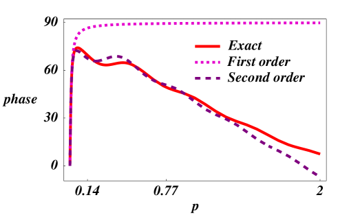
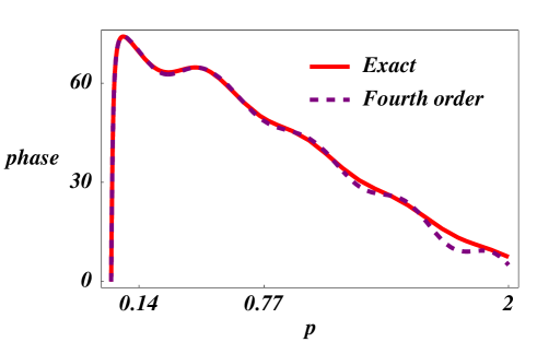
Figure 1: Leading (dotted)and subleading (dashed) EFT result for the toy model, compared with the exact answer (solid), plotted as degrees vs. $p=\sqrt{ME_{cm}}$ in GeV.

Figure 2: Fourth order EFT result (dashed) compared with the exact result (solid), plotted as degrees vs. $p=\sqrt{ME_{cm}}$ in GeV.

How quickly does the series converge to the true phase shift? I take $m_{\pi}=140$ MeV, $m_{\rho}=770$ MeV. In order to have the toy model resemble realistic $np$ scattering in the ${}^{1}S_{0}$ channel, I choose $a=-23$ fm, and set $\Lambda=500$ MeV so that the “pion” interaction in the toy model resembles the true one-pion exchange potential . In Fig. LABEL:comp12 I have plotted the first two terms in the KSW expansion (dashed lines) against the exact result (solid line). The lowest order (LO) result gets the scattering length exactly, but quickly fails to describe the “data”. The next-to-leading order (NLO) result is a vast improvement, working crudely up to $p\sim m_{\rho}$. In Fig. 2 I show the result at fourth order in the KSW expansion; it exhibits excellent agreement up to $p\sim m_{\rho}$, and shows not only that the expansion is converging rapidly (in spite of the enormous difference between LO and NLO results), but also that the radius of convergence in momentum is set by $m_{\rho}$ and not $m_{\pi}$.

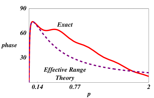
Figure 3: The effective range approximation for the phase shift in the toy model (dotted) compared with the exact result (solid), plotted as degrees vs. $p=\sqrt{ME_{cm}}$ in GeV. The approximation breaks down at $p\sim m_{\pi}$.

For comparison, I have plotted the effective range result in Fig. 3. It does an excellent job at describing the true phase shift for $p<m_{\pi}$ (better than the NLO EFT result), but fails as one would expect above $p\sim m_{\pi}$

Recently several papers have appeared suggesting that pions must be included nonperturbatively in order to obtain convergent answers above $p\sim m_{\pi}$ [8, 9, 10]. This does not appear to be the case in the toy model, and I don’t believe it is true for the real world. Instead, I think one gets into trouble by trying to exactly reproduce the effective range expansion parameters $a$ and $r_{0}$ at finite order in the KSW expansion. That is because one is forcing the short range physics to account for the contributions to these observables from neglected higher order pion exchange. By incorrectly determining the short distance physics (which is finely tuned), one runs into trouble at higher momentum. In the toy model considered here, choosing the $C_{2n}$ coupling to exactly reproduce the $(n+1)$ term in the effective range expansion yields an EFT prediction that fails (at any order in the expansion) at $p\sim m_{\pi}$. These issues are to be discussed at greater length in Ref. [11].

4 The real world

I will now briefly describe the status of calculations for real two and three nucleon physics using the KSW expansion. Phase shifts have been fit to NLO [2] in both the ${}^{1}S_{0}$ and ${}^{3}S_{1}-{}^{3}D_{1}$ channels, as shown in Fig. 4.

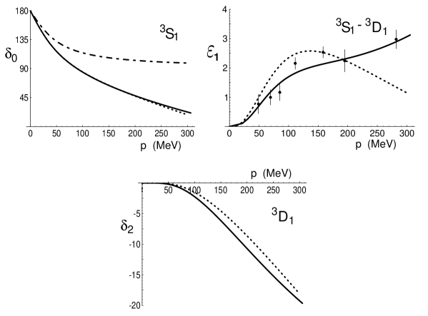
Figure 4: $NN$ phase shifts from Ref. [2]. The dot-dash and dotted lines are the LO and NLO EFT results respectively. The solid lines are from the Nijmegen partial wave (multi-energy) analysis; the data points for $\epsilon_{1}$ are from a single-energy analysis [12].

Using the $C$ parameters derived from the $NN$ phase shifts, a number of two-nucleon processes have been computed. In Figs. (5,6) I show results for the electromagnetic form factors of the deuteron from Ref. [7].

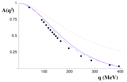
Figure 5: Electric form factor of the deuteron. The dotted and solid curves are the LO and NLO effective field theory results respectively; the dashed curve is the effective range theory prediction. The data are from various sources [7].

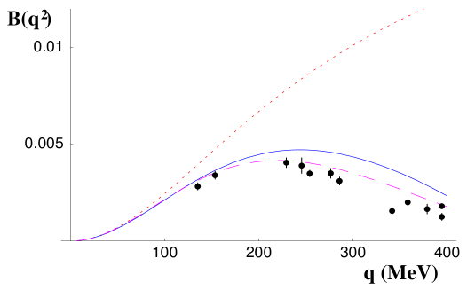
Figure 6: Magnetic form factor of the deuteron. The dotted and solid curves are the LO and NLO effective field theory results respectively; the dashed curve is the effective range theory prediction [7].

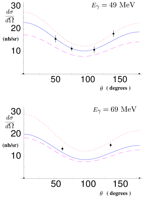
Figure 7: Angular distribution for Compton scattering off the deuteron, for two different energies. In each case the dashed (red) curves represent the LO result; the solid (blue) curves are the full NLO result. The dotted (red) curves are the NLO result when nucleon polarizability graphs are omitted. From Ref. [13].

These figures give evidence that the KSW expansion is converging. However, it also shows that conventional effective range theory gives a somewhat better fit to the data than does the EFT calculation at NLO. Presumably this is because the effective range approximation is fit to reproduce low energy scattering data exactly, while the EFT calculation yields low energy amplitudes in an expansion in powers of $\sim m_{\pi}/\Lambda\sim 1/3$.

In Fig. 7 is displayed the result from Ref. [13] for Compton scattering off the deuteron. Recently $np$ capture has been examined, both the parity conserving part to NLO [14], and the parity violating part to LO Ref. [15]. All of these calculations have been performed analytically. To give you an idea what is involved, I display in Fig. 8 the graphs that had to be computed for the calculation of parity violation in $np$ capture.

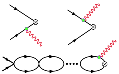
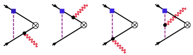
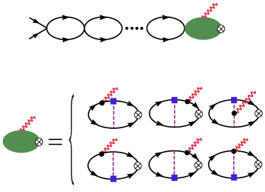
Figure 8: Feynman diagrams contributing to parity violating $np$ capture to lowest order, from Ref. [15]. The square vertex arises from the weak interactions.

Other two-nucleon EFT calculations using the KSW expansion include the deuteron anapole moment[16] and polarizability[17].

Figure 9: $N-d$ scattering phase shift, $J=3/2$ channel, computed in EFT. The only input are the two-body $J=1$ scattering length and effective range. From Ref. [19].

The most interesting challenge in nuclear effective theory presently is to extend the analysis to nuclear matter or finite nuclei. There are a number of issues that arise in the three-body system that must be understood before progress can be made. The simplest three-nucleon process to consider is $Nd$ scattering in the $J=3/2$ channel. This was recently computed in Refs. [18, 19] and the result is displayed in Fig. 9. Great progress has also been made in understanding the more interesting $J=1/2$ channel from the EFT perspective[20]. The problem is that the graphs one must compute must be represented as an integral equation, and no systematic power counting has yet been developed , although many interesting features have been understood. Understanding this system promises to be rewarding.

5 Discussion

How does the EFT approach measure up to conventional nuclear physics, where one solves the Schrödinger equation with a phenomenologically derived potential? So far, the LO and NLO calculations performed in the past nine months are not of comparable accuracy. Potential models obviously do much better than EFT at fitting $NN$ phase shifts, as they typically have about two dozen parameters expressly tuned to fit the data. What about other quantities?

• Deuteron electric moments: State-of-the-art potential models also do quite well at explaining quantities particularly sensitive to long distance physics. This includes the deuteron charge radius and magnetic moments, accurate to $\sim 1\%$ [23]. In contrast, the EFT predictions for the deuteron charge radius are off by $28\%$ at LO, and by $11\%$ at NLO [7]. The reason for this rather poor agreement is that even low momentum properties get corrections order by order in the KSW expansion. The deuteron quadrupole moment is off by $6\%$ in potential model calculations[23]; only the LO result from EFT has been obtained to date, and it is off by $39\%$.

• Deuteron polarizability: The polarizability of the deuteron has not been measured, but different potential models agree with each other on the value of the scalar electric polarizability to $\sim 0.3\%$ [21]; the EFT calculation differs from the potential model results by $\sim 39\%$ at LO, and $6\%$ at NLO.

• Deuteron Compton scattering: Compton scattering in the energy range shown in Fig. 7 is less sensitive to the very long range features of the deuteron wavelength. Predictions from potential models [22] agree with the data at the $\sim 10\%$ level, which is comparable to the agreement found in the NLO EFT calculation.

My conclusion is that the operative expansion parameter in the KSW expansion is $\sim 1/3$, with LO results agreeing with data to the 30% level and NLO agreeing to the 10% level. NLO calculations are typically not very arduous, and can usually be obtained in closed, analytic form. An important NLO calculation yet to be performed is the quadrupole moment of the deuteron. I expect that NNLO calculations, expected to be accurate to $\sim 3\%$, will prove to be competitive with — and in some cases, superior to — potential model calculations for a wide variety of two nucleon processes. Such calculations involve relativistic corrections and propagating pions, and have not yet been fully understood, although several groups are working on the problem. NNLO results most competitive with potential model results will be those relatively insensitive to the long wavelength tail of the deuteron wave function. Perhaps a better understanding of how in practice to match the KSW expansion to the effective range expansion at very low energies could improve the predictions for the latter observables.

Extending the EFT approach to few- and many-body systems remains an intriguing challenge, one that must be surmounted before EFT can really be of much use in nuclear theory. Like civilizations, physics theories progress from barbarism, to civilization to decadence (occasionally skipping the civilized state). Nuclear effective theory is still in the barbaric stage. Nevertheless, great progress has been made over the past nine months, and I am optimistic that the techniques will catch on and eventually prove themselves invaluable.

References

- [1] S. Weinberg, Phys. Lett. B 251, 288 (1990); Nucl. Phys. B 363, 3 (1991)
- [2] D.B. Kaplan, M.J. Savage and M.B. Wise, Phys. Lett. B 424, 390 (1998); Nucl. Phys. B 534, 329 (1998)
- [3] U. van Kolck, hep-ph/9711222
- [4] M. Luke and A.V. Manohar, Phys. Rev. D 55, 4129 (1997).
- [5] J. Gegelia, nucl-th/9802038
- [6] T. Mehen, I. W. Stewart, nucl-th/9809095
- [7] D.B. Kaplan, M.J. Savage, and M.B. Wise, nucl-th/9804032, to appear in Phys. Rev. C
- [8] J. Gegelia, nucl-th/9806028
- [9] T.D. Cohen, J. M. Hansen, nucl-th/9808006; nucl-th/9808038
- [10] J. V. Steele, R.J. Furnstahl, nucl-th/9808022
- [11] D.B. Kaplan, J.V. Steele, in preparation.
- [12] V.G.J. Stoks, R.A.M. Klomp, C.P.F. Terheggen and J.J. de Swart, Phys. Rev. C49 (1994) 2950,
- [13] J.-W. Chen, H. W. Griesshammer, M. J. Savage, R.P. Springer, Nucl. Phys. A 644, 245 (1998)
- [14] M. J. Savage, K. A. Scaldeferri, M. B. Wise, nucl-th/9811029.
- [15] D.B. Kaplan, M.J. Savage, R.P. Springer, M.B. Wise, nucl-th/9807081, submitted to Phys. Lett. B.
- [16] M.J. Savage, R.P. Springer, Nucl. Phys. A 644, 235 (1998)
- [17] J.-W. Chen, H.W. Griesshammer, M.J. Savage, R.P. Springer, Nucl. Phys. A 644, 221 (1998)
- [18] P.F. Bedaque, U. van Kolck, Phys. Lett. B 428, 221 (1998)
- [19] P.F. Bedaque, H.W. Hammer, U. van Kolck, Phys. Rev. C 58, R641 (1998)
- [20] P.F. Bedaque, H.W. Hammer, U. van Kolck, nucl-th/9806025; nucl-th/9811046
- [21] J.L. Friar, G.L. Payne, Phys. Rev. C 55, 2764 (1997)
- [22] T. Wilbois, P. Wilhelm, H. Arenhovel, Few Body Syst. Suppl. 9, 263 (1995); M.I. Levchuk, A.I. L’vov, Few Body Syst. Suppl. 9, 439 (1995)
- [23] B.S. Pudliner, V.R. Pandharipande, J. Carlson, S.C. Pieper, R.B. Wiringa, nucl-th/9705009
- [24] M. Rho, nucl-th/9812012