Real Time Dynamics of Colliding Gauge Fields and the ”Glue Burst”

Abstract

The Yang Mills equations provide a classical mean field description of gauge fields. In view of developing a coherent description of the formation of the quark gluon plasma in high energetic nucleus-nucleus collisions we study pure gauge field dynamics in 3+1 dimensions. In collisions of wave packets, numerically simulated on a SU(2) gauge lattice, we study transverse and longitudinal energy currents. For wave packets with different polarizations in color space, we observe a time delayed fragmentation after the collision resulting in a rapid expansion into transverse directions. We call this phenomenon the ”glue burst”. An analysis of the Yang Mills equations reveals the explanation for this behavior. We point out that this effect could play a role in ultra-relativistic heavy-ion collisions.

I Introduction

It is one of the most challenging topics in the theory of ultra-relativistic heavy-ion collisions to develop a coherent description of the formation of the quark gluon plasma. Many descriptions of the time evolution of such collisions have been developed in the past years [1, 2, 3, 4, 5]. Some of the most recent are the ultra-relativistic quantum molecular dynamics model (UrQMD) [1] and the parton cascade model [6]. While the UrQMD has been developed for collisions at center of mass energies below $10\,{\rm GeV/u}$, the parton cascade model is valid for energies at and above $100\,{\rm GeV/u}$ where the transition into the plasma phase is expected to occur. Both are based on the idea of a perturbative scattering of particles within transport models and describe in principle the evolution of a collision from the first contact of the nuclei throughout the high density phase until to the point where the last Hadrons are freezing out. These models however contain still a variety of problems. One of the problems concerns the description of the initial state of the colliding nuclei. The transport equations start from probability distributions of partons in the phase space. In reality however, the states of the nuclei are described through coherent parton wave functions. The incoherent parton description especially breaks down at exchanges of small transverse momenta. A few years ago, McLerran and Venugopalan proposed [7] that the proper solution of these difficulties is the perturbative expansion not around the empty QCD vacuum but around a vacuum of the mean color fields which accompany the quarks in the colliding nuclei. This idea motivates the development of a combination of the parton cascade model [6] with a coherent description of the initial states. This difficult goal can be accomplished in small steps through systematic studies. Recently, we have proposed a combination of a gauge lattice description for the soft color fields with a transport model for color charged particles [8]. Leaving out the collision terms first, this model then has been applied to simulate the collision of clouds of color charged particles accompanied by soft color fields in 3+1 dimensions [9]. The field energy distributions obtained for times shortly after the collision have shown transverse energy flows resulting from glue field scattering in the center of collision. For times larger than $1\,{\rm fm/c}$ glue field radiation seemed to be dominant. The sudden appearance of transverse energy flows during the overlap time of the nuclei was the motivation to study here the pure glue mean field dynamics leaving out the particles. The time evolution of colliding Yang Mills field wave packets has been studied a few years ago in 1+1 dimensions [10]. These calculations have shown that wave packets of equal polarization in color space (Abelian case) do not interact whereas wave packets polarized into different color directions (non-Abelian case) decay after the collision into low frequency modes of high particle multiplicity in the sense of Ref. [11, 12]. This mechanism of a coupling between high frequency short wavelength modes and low frequency long wavelength modes in the Yang Mills equations has also been observed in Ref. [13].

In the present paper, we focus on the transverse dynamics and the coupling between longitudinal and transverse energy flows in collisions of Yang Mills fields. A study of the transverse dynamics requires simulations in at least 2+1 dimensions. Subsequently, we describe the method used to solve the Yang Mills equations and present results obtained from collisions simulated in 3+1 dimensions on a SU(2) gauge lattice. These studies also reveal an interesting behavior of the time-evolution of non-Abelian gauge fields.

II Time Evolution on the Gauge Lattice

In the Lie algebra LSU(2), we define the adjoint gauge fields ${\cal A}^{\mu}(x):=A_{c}^{\mu}(x)T^{c}$ and the adjoint field strength tensor ${\cal F}^{\mu\nu}:=F^{\mu\nu}_{c}T^{c}$. Einsteins sum convention has to be applied in the Euclidean metric for upper and lower color indices and in the Mincowski metric for upper and lower greek indices. The symbols $T^{c}$ with color index $c=1,2,3$ denote the generators of LSU(2) obeying the commutation relations $\bigl{[}T^{a},T^{b}\bigr{]}_{-}=if_{abc}T^{c}$ and hence ${\cal A}^{\mu}(x),{\cal F}^{\mu\nu}\in$ LSU(2) for all $x\epsilon{\bf R}^{4}$. Here, we chose the representation $T^{c}=1/2\,\sigma^{c}$ with the Pauli matrices $\sigma^{c}$. Further below, we use also $T^{0}:={1\over 2}{\bf 1}_{2}$ which is linearly independent from the generators $T^{c}$. With these conventions, we denote the Yang Mills equations in the short form

$$\bigl{[}{\cal D}_{\mu},{\cal F}^{\mu\nu}\bigr{]}_{-}=0,$$ (1)

where ${\cal D}_{\mu}$ is defined

$${\cal D}_{\mu}:=\partial^{\mu}-ig{\cal A}^{\mu}.$$ (2)

With this definition of the covariant derivative ${\cal D}_{\mu}$ on the SU(2) mainfold, and with the definitions ${\cal E}^{\mu}(x):=E_{c}^{\mu}(x)T^{c}$, ${\cal B}^{\mu}(x):=B_{c}^{\mu}(x)T^{c}$ (${\cal E}^{\mu}(x),{\cal B}^{\mu}(x)\,\in$ LSU(2)) of the adjoint color electric and color magnetic field quantities, the Yang Mills equations Eq. (1) can be expressed in a form which is similar to the U(1) Maxwell equations in the vacuum

$$\bigl{[}{\vec{\cal D}},{\vec{\cal E}}\bigr{]}_{-} = 0,$$ (3)

$$\bigl{[}{\vec{\cal D}},{\vec{\cal B}}\bigr{]}_{-} = 0,$$ (4)

$$\bigl{[}{\vec{\cal D}}\times,{\vec{\cal E}}\bigr{]}_{-} = \bigl{[}{\cal D}_{0},{\vec{\cal B}}\bigr{]}_{-},$$ (5)

$$\bigl{[}{\vec{\cal D}}\times,{\vec{\cal B}}\bigr{]}_{-} = \bigl{[}{\cal D}_{0},{\vec{\cal E}}\bigr{]}.$$ (6)

With the condition $\bigl{[}{\cal A}(t,\vec{x}),{\cal A}(t,\vec{x}^{\prime})\bigr{]}_{-}=0$ for all $\vec{x},\vec{x}^{\prime}\in{\bf R}^{3}$ for one arbitrary real time $t$, the equations (3) to (6) are indeed identical with the Maxwell equations. In this so called Abelian (or U(1)) case, one expects a linear behavior of the solution and it therefore provides an important test through comparison with the solution in the general non-Abelian case. The Yang Mills equations can be solved in an efficient manner on a gauge lattice in a Hamiltonian framework where we choose the temporal gauge ${\cal A}^{0}=0$.

A lattice version of the continuum Yang Mills equations is constructed by expressing the color field amplitudes as elements of the corresponding Lie algebra, i.e. ${\cal E}_{{\vec{x}},k},{\cal B}_{{\vec{x}},k}\,\in$ LSU(2) at each lattice site $\vec{x}$. We define the following variables.

$${\cal U}_{{\vec{x}},l} = \exp(-iga_{l}{\cal A}_{l}(x))\,\,=\,\,{\cal U}^{\dagger}_{{\vec{x}}+l,-l}$$ (7)

$${\cal U}_{{\vec{x}},kl} = {\cal U}_{{\vec{x}},k}\,{\cal U}_{{\vec{x}}+k,l}\,{\cal U}_{{\vec{x}}+k+l,-k}\,{\cal U}_{{\vec{x}}+l,-l}$$ (8)

In adjoint representation the color electric and color magnetic fields are expressed in terms of the above defined link variables ${\cal U}_{{\vec{x}},l}$ and plaquette variables ${\cal U}_{{\vec{x}},kl}$ in the following way.

$${\cal E}_{{\vec{x}},j} = {{1}\over{iga_{j}}}\,\dot{\cal U}_{{\vec{x}},j}{\cal U}^{\dagger}_{{\vec{x}},j}$$ (9)

$${\cal B}_{{\vec{x}},j} = {{i}\over{4ga_{k}a_{l}}}\,\epsilon_{jkl}\,\bigl{(}{\cal U}_{{\vec{x}},kl}-{\cal U}^{\dagger}_{{\vec{x}},kl}\bigr{)}.$$ (10)

The lattice constant in the spatial direction $l$ is denoted by $a_{l}$. As one can see from (6), the gauge field ${\cal A}_{{\vec{x}},l}$ is expressed in terms of the link variables ${\cal U}_{{\vec{x}},l}\,\epsilon$ SU(2), which represent the parallel transport of a field amplitude from a site $x\,\epsilon\,X$ to a neighboring site $(x+l)\,\epsilon\,X$ in the direction $l$. We choose ${\cal U}_{{\vec{x}},i}$ and ${\cal E}_{{\vec{x}},i}$ as the basic dynamic field variables and numerically solve the following equations of motion.

$$\dot{\cal U}_{{\vec{x}},k}(t) = i\,g\,a_{k}\,{\cal E}_{{\vec{x}},k}(t)\,{\cal U}_{{\vec{x}},k}(t)$$ (11)

$$\dot{\cal E}_{{\vec{x}},k}(t) = {i\over{2ga_{1}a_{2}a_{3}}}\sum\limits^{3}_{l=1}\Bigl{\{}{\cal U}_{{\vec{x}},kl}(t)-{\cal U}^{\dagger}_{{\vec{x}},kl}(t)\,\Bigr{.}$$ (12)

$$- \Bigl{.}{\cal U}^{\dagger}_{{\vec{x}}-l,l}(t)\,\Bigl{(}{\cal U}_{{\vec{x}}-l,kl}(t)-{\cal U}^{\dagger}_{{\vec{x}}-l,kl}(t)\Bigr{)}\,{\cal U}_{{\vec{x}}-l,l}(t)\,\Bigr{\}}.$$ (13)

III Numerical Results

First, we study the collision of plane wave packets which have initially constant amplitude in the transverse planes of a 3-torus lattice implying periodic boundary conditions. The size is chosen 20x20x2000 lattice points. We denote the lattice spacing in the space direction $l$ by $a_{l}$. For a collision, we initially arrange wave packets of a Gaussian shape in the longitudinal direction. The average momenta of the wave packets are $(0,0,\pm\overline{k}_{3})$ and their momentum spread is denoted $\Delta k_{3}$. As a consequence of the lattice discretization these quantities are restricted to values between the maximal and minimal Fourier-momenta on the lattice:

$$k_{l}^{min}={\pi\over{(N_{l}a_{l})}},\qquad k_{l}^{max}={\pi\over{(N_{l}a_{l})}},$$ (14)

$$k_{l}^{min}\,\ll\,\Delta k_{l}\,\ll\,\overline{k}_{l}\,\ll\,k_{l}^{max}$$ (15)

The polarization in color space is defined by the unit vectors $\vec{n}_{\rm L}^{c}$ for the left (L) and $\vec{n}_{\rm R}^{c}$ for the and right (R) moving wave packet respectively.

We express the initial conditions through the gauge fields

$$A_{L}^{c}=\delta_{l1}{\vec{n}}^{c}_{L}\phi(+t,x_{3}-Z_{L}),$$ (16)

$$A_{R}^{c}=\delta_{l1}{\vec{n}}^{c}_{R}\phi(-t,x_{3}-Z_{R})$$ (17)

where the scalar function $\phi(t,x_{3})$ defines the initial wave packet

$$\phi(t,x_{3}) = \phi_{0}\exp{\bigl{(}-{1\over 2}\Delta k_{3}^{2}(t+x_{3})^{2}\bigr{)}}\cos{\bigl{(}\overline{k}_{3}(t+x_{3})\bigr{)}},$$ (18)

$$\phi_{0} = \sqrt{{(2\Delta k_{3})}/({\sqrt{\pi}\sigma\overline{k}_{3}})}\bigl{(}1+e^{-(\overline{k}_{3}/\Delta k_{3})^{2}}\bigr{)}$$ (19)

The amplitude factor $\phi_{0}$ is determined for a normalized wave packet when $\sigma=100a_{1}a_{2}$. The parameter $\sigma$ is used to control the amplitude and allows to adjust the energy contained in a wave packet. In a particle interpretation it describes the total cross section per particle contained in the wave packet [10]. The second term in $\phi_{0}$ is usually negligibly small for wave packets since $\overline{k}_{3}/\Delta k_{3}\gg 1$. We chose the polarizations in color space $\vec{n}_{R}=\vec{n}_{L}=(0,0,1)$ for the Abelian case and $\vec{n}_{R}=(0,0,1),\,\vec{n}_{L}=(0,1,0)$ for the non-Abelian case. Once the initial fields are mapped on the lattice, the time evolution of the collision starts from the superposed initial conditions

$${\cal U}^{(0)}_{{\vec{x}},l} = {\cal U}^{(0)}_{{\vec{x}},l,L}\cdot{\cal U}^{(0)}_{{\vec{x}},l,R},$$ (20)

$${\cal E}^{(0)}_{{\vec{x}},l} = {\cal E}^{(0)}_{{\vec{x}},l,R}+{\cal E}^{(0)}_{{\vec{x}},l,L},$$ (21)

respectively. A linear superposition of solutions obeys the Yang Mills equations only if these solutions have no overlap . Therefore, the initial separation $\Delta Z$ should be much larger than $1/{\Delta k_{3}}$.

The calculation contains four parameters. The relative color polarization which is parameterized by the angle $\theta_{\rm C}$ defined through $\vec{n}_{L}\cdot\vec{n}_{R}=\cos(\theta_{\rm C})$. The average momentum of the wave packets $\overline{k}$ and their width $\Delta k_{3}$ and the coupling constant $g$ which can be rewritten in terms of the parameter $\sigma$ as $g^{\prime}=g/\sqrt{\sigma}$ by simultaneously rescaling the field ${\cal A}$ as ${\cal A}^{\prime}=\sqrt{\sigma}{\cal A}$. Consequently, the system shows the same dynamics for different values of $g$ and $\sigma$, as long as the ratio $g^{\prime}=g/\sqrt{\sigma}$ is kept fixed. Multiplying the Eq. (33) in section 4 by a factor $g$, shows that each amplitude ${\cal A}^{\mu}$ absorbs a $g$ such that no $g$ is left over in Eq. (33). For $\overline{k}_{3}\gg\Delta k_{3}$, the energy contained in one wave packet is essentially $\overline{k}_{3}/\sigma$, i.e. for given $\overline{k}_{3}$ the energy is determined through the amplitude and vice versa the amplitude is thus fixed by the energy. Once the amplitude is fixed, it makes sense to use the coupling constant as an additional parameter which determines the reaction dynamics of colliding wave packets. This is preferable also in view of studies in the future where normalized Dirac fields or color charged classical particles shall be included. In such cases $g$ appears also in front of the source current of the inhomogeneous Yang Mills equations. We therefore keep the explicit denotation of $g$ in the subsequent sections.

In the following we present results from a simulated collision in the non-Abelian case with the parameters $\overline{k}_{3}=\pi/(2a_{3})$, $\Delta k_{3}=\pi/(100a)$, $g=1$, $\sigma=100a^{2}=1.0{\rm fm}^{2}$. The simulation was performed on a uniform lattice with constants $a_{1}=a_{2}=a_{3}=a$ using a time step size $\Delta t=a/10$. If we would consider a collision of nuclei at low energies, $a=0.1\,{\rm fm}$ would be an appropriate choice for the above parameter settings. In particluar, $\Delta k_{3}=\pi/(100a)$ corresponds thus to a FWHM of $10\,{\rm fm}$ which is approximately the diameter of a ${}^{208}Pb$-nucleus. It is important to note that for the above chosen values, the calculation runs in the regime of weak coupling. Subsequently, we refer to the direction of the collision axis as the ”longitudinal direction” and to directions perpendicular to the collision axis as the ”transverse directions”. Accordingly, we define the transverse and longitudinal energy densities of the color electric field

$$w_{T}^{(E)}(t,x_{3}) = \int dx_{1}dx_{2}\sum\limits_{l=1}^{2}{\rm Tr}\bigl{(}{\cal E}_{l}{(t,{\vec{x}})}{\cal E}_{l}{(t,{\vec{x}})}\bigr{)},$$ (22)

$$w_{L}^{(E)}(t,x_{3}) = \int\int dx_{1}dx_{2}{\rm Tr}\bigl{(}{\cal E}_{3}{(t,{\vec{x}})}{\cal E}_{3}{(t,{\vec{x}})}\bigr{)}$$ (23)

Fig. 1 displays $w_{T}^{(E)}$ plotted over the $x_{3}$-coordinate at various time steps $t_{n}$ as indicated on top of the curves.

FIG. 1.: Transverse energy densities $w_{T}^{(E)}(t,x_{3})$ are plotted over the collision axis (longitudinal coordinate) for selected time steps $t_{n}$.

At initial time $t_{0}$ the distributions $w_{T}^{(E)}(t_{0},x_{3})$ of the wave packets are completely filled resulting from the strong oscillations in the longitudinal direction according to $\overline{k}_{3}=\pi/(2a_{3})$. After 1500 time steps the wave packets are colliding and have reached maximum overlap. The smooth white zone at the bottom results from a phase shift between the two superposed waves, i.e. the maxima of the wave packet (1) to not coincide with the maxima of the wave packet (2) at time step $t_{1500}$. After the wave packets have passed through each other (at about $t_{2500}$), a small white zone remains in the distribution $w_{T}^{(E)}(x_{3})$ of each and keeps continuously growing. At time step $t_{6000}$ ($t=600a$) the large fraction of the initial high frequency oscillations is reduced to a small remaining contribution visible on the surface of the distibutions in Fig. 1. The hight of the two receding humps decreases accordingly while the energy carried by each wave packet is constant in time. Almost all the energy which has originally been carried by short wavelength modes around $\overline{k}_{3}$ has been transmitted into long wavelength modes which have filled up the vallies in the oscillating distribution $w_{T}^{(E)}(x_{3})$. This behavior agrees qualitatively with results obtained in Ref. [10] where collisions of wave packets have been studied on a one dimensional gauge lattice and for times not larger $t=600a$. At time step $t_{8000}$ however, we observe that energy is partly transmitted back into high frequent modes before the wave packets start to decay around time step $t_{10000}$. At time step $t_{14000}$, the energy distribution has expanded into longitudinal direction. The appearance of a circular polarization of the receding wave packtes could in princple lead to the same behavior before they decay. This possibility, however, is excluded by our numerical results which show - in the case of plane waves - no excitation of modes with $x_{2}$-polarization for all times. This can be veryfied down to floating point precision but it has also a fully analytic explanation through Eq. (33) in section 4 for $\nu=2$.

This behavior does not appear in a collision of wave packets which are equally polarized in color space. In this case the shape of the two humps in the distribution $w_{T}^{(E)}(x_{3})$ at the time step $t_{14000}$ is almost identical with the shape at time $t_{0}$. Deviations result from lattice dispersion.

FIG. 2.: Longitudinal energy densities $w_{L}^{(E)}(t,x_{3})$ are plotted over the collision axis (longitudinal coordinate) for selected time steps $t_{n}$

In Fig. 2, the corresponding longitudinal energy densities $w_{L}^{(E)}(t,x_{3})$ are displayed on a logarithmic scale for selected time steps $t_{n}$. We remember that the wave packets were initially polarized into the transverse $x_{1}$-direction and consequently $w_{L}^{(E)}$ has to be zero as long as they propagate free. However, when the colliding wave packets of different color start overlapping, we observe an increasing longitudinal energy density in the overlap region around the center of collision at $x_{3}=100\,{\rm fm}$. Fig. 2 clearly shows that $w_{L}^{(E)}(t,z)$ grows rather fast from time step $t_{1000}$ until time step $t_{1500}$ where it reaches a maximum and has grown by more than two orders of magnitude. For larger times the hump decreases again and practically disappears at $t_{3000}$. Around $t_{6000}$, however, the longitudinal energy density grows again at the positions of the receding wave packets. After 10000 time steps $w_{L}^{(E)}(z)$ has increased by five orders of magnitude.

A comparison of Fig. 1 with Fig. 2 indicates that the total color electric field energy on transverse links of the lattice decreases at large times while the total color electric field energy on longitudinal links increases. In order to understand this behavior in detail, we explore the time dependence of these quantities for different values of the coupling constant. To be more precise, we define the transverse and longitudinal energy of the color electric fields as

$$W_{T}^{(E)}(t) = \int d^{3}x\sum\limits_{l=1}^{2}{\rm Tr}\bigl{(}{\cal E}_{l}({t,\vec{x}}){\cal E}_{l}{({t,\vec{x}})}\bigr{)},$$ (24)

$$W_{L}^{(E)}(t) = \int d^{3}x{\rm Tr}\bigl{(}{\cal E}_{3}{({t,\vec{x}})}{\cal E}_{3}{({t,\vec{x}})}\bigr{)}$$ (25)

The integration in the definitions (24) and (25) is carried out over the whole lattice.

Fig. 3 displays $W_{T}^{(E)}(t)$ over a time interval of $600a$ which corresponds to 6000 time steps. The energies are compared for different values of the coupling constant $g$. As already mentioned above, values of the coupling constant which differ from $g=1$ can be scaled out with the amplitude of the wave functions. The amplitude of wave packets, however, determines the energy carried by a wave. Once the energy is fixed by describing a real physical system, it makes sense to use different values of the coupling constant. Here, we collide wave packets which are normalized to ${N_{1}N_{2}a^{2}}/\sigma$ particles and refer to different values of $g$.

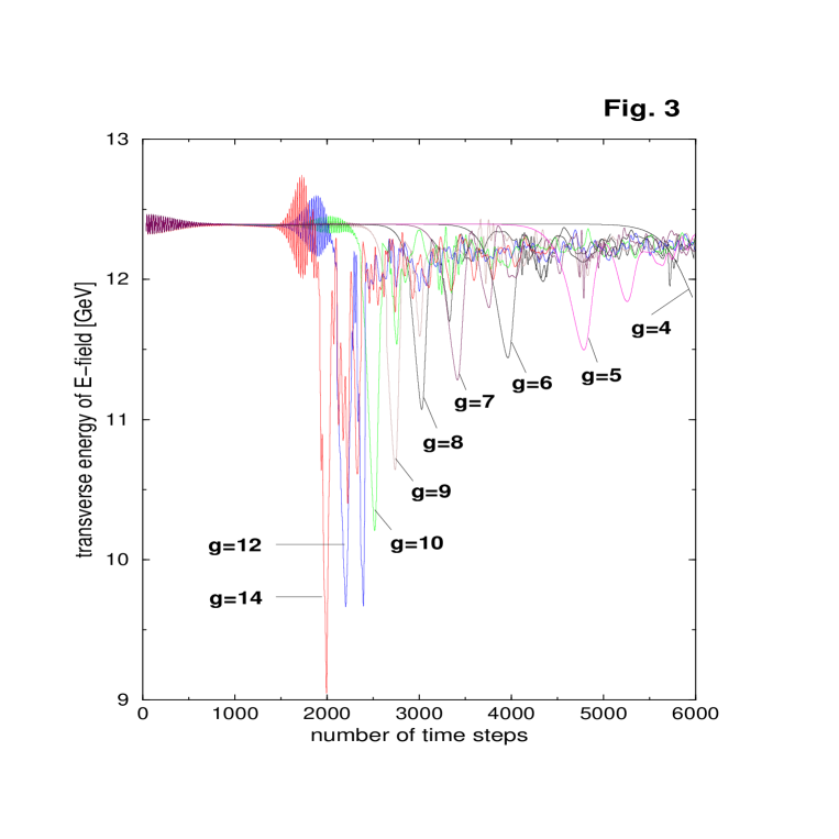
FIG. 3.: The transverse color electric field energy $W_{T}^{(E)}(t)$ as a function of time is displayed for different values of the coupling constant $g$. The time step width of each time step is $\Delta t=a_{3}/10=0.01\,{\rm fm}$.

Fig. 3 shows that for small coupling, $W_{T}^{(E)}(t)$ remains unchanged through a long period of time after the collision which occurs in an interval around the time step $t_{1500}$. For $g=4$ the transverse color electric energy starts to decrease around time step $t_{5000}$. A comparison with curves obtained for increasing values of $g$ shows that the $W_{T}^{(E)}(t)$ begins to decrease at earlier times. For the largest values $g=10,12,14$, the decrease begins in the overlap region of the wave packets. In these cases, strong oscillations occur in the overlap region. The magnetic field energies $W_{T}^{(B)}(t)$ show a very similar behavior. The total energy of both wave packets is $24.76\,{\rm GeV}$ for our numerical choice $a=0.1\,{\rm fm}$.

Fig. 4 displays the corresponding longitudinal field energy $W_{L}^{(E)}(t)$. Before the wave packets start to overlap we find $W_{L}^{(E)}(t)=0$ to a very high precision ($10^{-26}$). In the overlap region, a hump like structure occurs which grows for increasing values of $g$. For small values of $g$, $W_{L}^{(E)}(t)$ vanishes after the wave packets have passed through each other. After a long time $W_{L}^{(E)}(t)$ grows very steeply. Fig. 4 shows clearly that the time between overlap and sudden growth shrinks for increasing coupling $g$. We find, that this time difference scales like $1/g^{2}$.

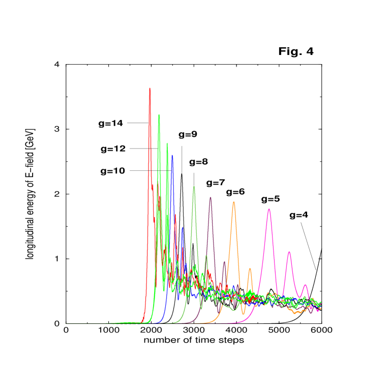
FIG. 4.: The longitudinal color electric field energy $W_{L}^{(E)}(t)$ as a function of time is displayed for different values of the coupling constant $g$. The time step width of each time step is $\Delta t=a_{3}/10=0.01\,{\rm fm}$.

Now the question arises whether the energy deposit in longitudinal links can be associated with fields propagating into transverse directions. To define energy currents, we denote the Poynting vector in the adjoint representation

$$\vec{\cal S}:=c\,\vec{\cal E}\times{\cal B}.$$ (26)

With the transverse and longitudinal components of the vector (26) we define the total transverse and longitudinal energy currents

$$i_{T}(t):=\sum_{l=1}^{2}\int d^{3}x2\,\big{|}{\rm Tr}\bigl{(}{\cal S}_{l}(t,\vec{x})\bigr{)}\big{|}$$ (27)

$$i_{L}(t):=\sum_{l=3}^{3}\int dx^{3}2\,\big{|}{\rm Tr}\bigl{(}{\cal S}_{l}(t,\vec{x})\bigr{)}\big{|}.$$ (28)

In the following Fig. 5, we show the total transverse energy current $i_{T}(t)$ in the overlap time region for different values of the coupling constant. The figure shows that there is no transverse energy current before the wave packets start to overlap. In the overlap time region between the time steps $t_{800}$ and $t_{1500}$, we observe a strong increase of the transverse energy current. The maximum is reached at time step $t_{1500}$ where the overlap is maximal. At decreasing overlap in time region between $t_{1500}$ and $t_{2200}$, $i_{T}(t)$ vanishes. The height of the humps increases for increasing values of $g$ and scales like $1/g^{2}$. To become more precise, in the time region of the humps as shown in Fig. 5, the transverse current implies an oscillating structure of the time period $T_{t}=\overline{\lambda}/4$ over which we have averaged to obtain the smooth curves in Fig. 5. $\overline{\lambda}$ is here defined as $\overline{\lambda}={(2\pi)/k_{3}}$ In the upper left panel in Fig. 5, we show an example for $\overline{k}_{3}=\pi/(4a_{3})$ in the case $g=8$ in which no averaging has been done. The curve displays a period of $T_{t}=2a_{3}$ according to $\overline{\lambda}=8a_{3}$. No averaging was necessary for times after the overlap time region.

FIG. 5.: The total transverse energy current $i_{T}(t)$ as a function of time is displayed for different values of the coupling constant g. The average longitudinal momentum of the colliding wave packets is $\overline{k}_{3}=\pi/(2a_{3})$. In the upper left window, the full time-dependence of the transverse energy current is displayed at the example $g=8$ and $\overline{k}_{3}=\pi/(4a_{3})$.

Fig. 6 displays the same transverse energy currents as Fig. 5 but for a larger time interval and on a larger scale. Note that the current is plotted in units of $[i_{T}(t)]=c\,{\rm GeV}$ in Fig. 6 but in units $[i_{T}(t)]=c\,{\rm MeV}$ in Fig. 5. After passing through the hump region between time step $t_{800}$ and $t_{2000}$, the energy current $t_{T}(t)$ disappears. For the smallest coupling $g=4$, it takes about 3500 time steps or $\tau\simeq 35\,{\rm fm}$ from maximum overlap until to the point where $i_{T}$ starts to re-grow. This time, $i_{T}$ grows to much larger values and stays large at later times. The time delay $\tau$ depends on $g,\Delta k_{3},\overline{k}_{3}$. We find that $\tau\sim 1/g^{2}$ but haven’t studied carefully the dependence on $\Delta k_{3}$ and $\overline{k}_{3}$. For large $\overline{k}_{3}$ at least, one can argue analytically that $\tau\sim{\overline{k}_{3}}^{-3/4}$. This will be further discussed in the appendix B. Some few calculations for smaller $\overline{k}_{3}$ have shown that $\tau$ increases monotonically for decreasing $\overline{k}_{3}$. The sudden increase of $i_{T}$ defines the “glue burst”. For large coupling it occurs already in the overlap region.

FIG. 6.: Same as in Fig. 5 but for a larger time intervall and on a larger scale for the transverse energy current $i_{T}(t)$.

The following Fig. 7 displays the corresponding longitudinal energy currents $i_{L}(t)$. It shows that $i_{L}$ decreases at the same time when $i_{T}$ increases.

FIG. 7.: The longitudinal energy currents $i_{L}(t)$ corresponding to the cases shown in Fig. 6 are displayed. $i_{L}(t)$ decreases at the same time when $i_{T}(t)$ increases.

Subsequently, we present some results from the collision of wave packets with a finite transverse extent. We have carried out similar calculations as in the case of plane waves and found a similar, but even more pronounced behavior for the time dependence of the transverse and longitudinal energy currents. Most of the calculations were carried out on a lattice of the size 4x200x800 points. The wave packets have been initialized in the same way as in the case for plane wave packets. However, the initial wave functions depend now also on the transverse coordinates. Since a lattice with the same extension in both transverse directions would lead to an exceedingly large number of lattice points, we chose a small number of lattice points in the $x_{1}$-direction. Thus, we study the dynamics of a collision in the $(x_{2},x_{3})$-plane integrated over the $x_{1}$-coordinate. Under these restrictions, the scalar function $\phi(t,x_{2},x_{3})$ defines the initial wave packet

$$\phi(t,x_{2},x_{3}) := \phi_{0}\exp{\bigl{(}-{1\over 2}\Delta k_{3}^{2}(t+x_{3})^{2}\bigr{)}}\exp{\bigl{(}-(\Delta k_{2}x_{2})^{\alpha}\bigr{)}}\cos{\bigl{(}\overline{k}_{3}(t+x_{3})\bigr{)}},$$ (29)

$$\phi_{0} := \sqrt{{(2\Delta k_{3})}/({\sqrt{\pi}\sigma\overline{k}_{3}})}.$$ (30)

The additional factor $\exp{\bigl{(}-(\Delta k_{2}x_{2})^{\alpha}\bigr{)}}$ describes the shape of the wave packet in the transverse $x_{2}$-direction. The parameter $\Delta k_{2}$ determines the transverse width and the parameter $\alpha$ controls the transverse shape. For large values of $\alpha$, we obtain a sharp surface and the exponential tails are suppressed. Since the transverse extension of the lattice is limited, we choose the extension of the initial wave packet in the $x_{2}$-direction small enough to leave space for the transverse dynamics after the collision. Good values are $\Delta k_{2}=1/(40a_{2})$ and $\alpha=8$. The wave packet is thus $8\,{\rm fm}$ wide and extends over 80 lattice points into the main transverse direction. Further outside the amplitude is practically zero since $\alpha$ is large. For $\Delta k_{3}=\pi/(100a_{3})$, the FWHM in longitudinal direction is $10\,{\rm fm}$.

With the function $\phi(t,x_{2},x_{3})$ we determine the initial link variables and the color electric field amplitudes and map these data on the lattice at the initial positions of the wave packets. For a collision, the wave packets have opposite average momenta $\pm\overline{k}_{3}$. The evolution of the collision is carried out in the same way as for plane wave packets. Fig. 8, shows snapshots of the transverse energy density of the color electric fields which we define as

$$w_{T}^{(E)}(t,x_{2},x_{3}) = \int dx_{1}\sum\limits_{l=1}^{2}{\rm Tr}\bigl{(}{\cal E}_{l}(t,\vec{x}){\cal E}_{l}(t,\vec{x})\bigr{)}.$$ (31)

The simulation shown in Fig. 8 has been carried out for the non-Abelian case and with a coupling $g=6$. The other parameter settings are as for plane waves above. The upper left picture shows the distribution for the time step $t_{100}$ where the shape has almost not changed as compared to the initial distribution. The wave packets decay into the transverse directions while they propagate free over the lattice. The upper right picture displays $w_{T}^{(E)}(t_{1500},x_{2},x_{3})$ at maximum overlap. In the middle left $w_{T}^{(E)}(t_{3500},x_{2},x_{3})$ is displayed. The distribution is almost identical with that obtained in the Abelian case at the same time step $t_{3500}$. At the time step $t_{4000}$, however, the waves packets start to burst. The last two images correspond to the time steps $t_{5000}$ and $t_{6000}$.

FIG. 8.: The transverse color electric field energy density $w_{T}^{(E)}(t,x_{2},x_{3})$ is shown for six selected snapshots taken at the time steps $t_{100}$, $t_{1500}$, $t_{3500}$, $t_{4000}$, $t_{5000}$ and $t_{6000}$. The corresponding pictures are ordered from the upper left to the lower right.

Note: The Fig.8 exceeds the size accepted at the lanl-server and was therefore omitted. We recommend to download the postscript file from the web page http://www.phy.duke.edu/~poeschl/ under “Rsearch Related Links” and “Preprints”.

IV Analysis of the Yang Mills Equations

In the following, we present the explanation of the glue burst solution by analyzing the Yang Mills equations (1). The details of the discussion are presented in the appendix A. With the definition of the field tensor ${\cal F}^{\mu\nu}:={\cal D}^{\mu}{\cal A}^{\nu}-{\cal D}^{\nu}{\cal A}^{\mu}$ , we rewrite Eq. (1) for the gauge fields in the adjoint denotation

$$\bigl{[}{\cal D}_{\mu},\bigl{(}{\cal D}^{\mu}{\cal A}^{\nu}-{\cal D}^{\nu}{\cal A}^{\mu}\bigr{)}\bigr{]}_{-}=0$$ (32)

With the definition of the derivative ${\cal D}^{\mu}$ in Eq. (2) follows

$$\partial_{\mu}\partial^{\mu}{\cal A}^{\nu} = \partial_{\mu}\partial^{\nu}{\cal A}^{\mu}\,+\,ig\partial_{\mu}\bigl{[}{\cal A}^{\mu},{\cal A}^{\nu}\bigr{]}_{-}$$ (33)

$$+ ig\bigl{[}{\cal A}_{\mu},\partial^{\mu}{\cal A}^{\nu}\bigr{]}_{-}$$ (34)

$$- ig\bigl{[}{\cal A}_{\mu},\partial^{\nu}{\cal A}^{\mu}\bigr{]}_{-}$$ (35)

$$+ g^{2}\bigl{[}{\cal A}_{\mu},\bigl{[}{\cal A}^{\mu},{\cal A}^{\nu}\bigr{]}_{-}\bigr{]}_{-}$$ (36)

Since the time delayed burst-like behavior of the solution occurs also in the case of colliding plane wave packets, we first consider this case. The phenomenon occurs in two steps. It is based on a delicate interplay of color degrees of freedom between the color sub-spaces ${\rm span}(T_{1},T_{2})$ and ${\rm span}(T_{3})$ and between transverse and longitudinal degrees of freedom in the field amplitudes.

The first step occurs in the overlap region of the wave packets in both, time and space. The Yang Mills equations provide a mechanism which transfers field energy from transverse into longitudinal field degrees of freedom. It is explained by the equation for the longitudinal gauge field components which follows from Eq. (33) for ${\nu=3}$. For plane wave packets, only the fourth term and the $g^{2}$-term do not vanish on the r.h.s. of Eq. (33) in the case $\nu=3$ and therefore the equation

$$\partial_{\mu}\partial^{\mu}{\cal A}^{3} = \,-\,ig\bigl{[}{\cal A}_{\mu},\partial^{\nu}{\cal A}^{\mu}\bigr{]}_{-}$$ (38)

$$\,+\,g^{2}\bigl{[}{\cal A}_{\mu},\bigl{[}{\cal A}^{\mu},{\cal A}^{\nu}\bigr{]}_{-}\bigr{]}_{-}$$

describes the dynamics of the longitudinal fields ${\cal A}^{3}$ during the overlap time. Assuming that $\big{|}A_{\mu}^{3}A^{\mu}_{3}\big{|}\ll\big{|}A_{\mu}^{1}A^{\mu}_{1}\big{|}$ and $\big{|}A_{\mu}^{3}A^{\mu}_{3}\big{|}\ll\big{|}A_{\mu}^{2}A^{\mu}_{2}\big{|}$ during the overlap time, we find the following leading contributions on the r.h.s. of Eq. (38).

$$-ig\bigl{[}{\cal A}_{\mu},\partial^{3}{\cal A}^{\mu}\bigr{]}_{-} \simeq {g}\bigl{(}A_{\mu}^{1}\partial^{3}A_{2}^{\mu}-A_{\mu}^{2}\partial^{3}A_{1}^{\mu}\bigr{)}T_{3}$$ (39)

$$g^{2}\bigl{[}{\cal A}_{(1)},\bigl{[}{\cal A}^{(1)},{\cal A}^{(3)}\bigr{]}_{-}\bigr{]}_{-} = \,{{g^{2}}}A_{(1)}^{1}A_{1}^{(1)}A_{3}^{(3)}\,T^{3}\,-\,{{g^{2}}}A_{(1)}^{3}A_{1}^{(1)}A_{3}^{(3)}\,T^{1}$$ (41)

$$\,+\,{{g^{2}}}A_{(1)}^{2}A_{2}^{(1)}A_{3}^{(3)}\,T^{3}\,-\,{{g^{2}}}A_{(1)}^{3}A_{2}^{(1)}A_{3}^{(3)}\,T^{2}$$

The above assumption is certainly true for the numerical results presented in the previous section which have demonstrated that in the overlap time the longitudinal energy densities are smaller by at least one order of magnitude in comparison to the transverse energy densities. The indices of the space coordinates in Eq. (41) are now denoted in parentheses in order to distinguish from color indices. In leading approximation, the dynamics of the longitudinal fields in the overlap time is thus described by the following equation

$$\partial_{0}\partial^{0}{\cal A}^{3} \simeq {g}\bigl{(}A_{\mu}^{1}\partial^{3}A_{2}^{\mu}-A_{\mu}^{2}\partial^{3}A_{1}^{\mu}\bigr{)}T_{3}$$ (44)

$$\,+\,{{g^{2}}}A_{(1)}^{1}A_{1}^{(1)}A_{3}^{(3)}\,T^{3}\,-\,{{g^{2}}}A_{(1)}^{3}A_{1}^{(1)}A_{3}^{(3)}\,T^{1}$$

$$\,+\,{{g^{2}}}A_{(1)}^{2}A_{2}^{(1)}A_{3}^{(3)}\,T^{3}\,-\,{{g^{2}}}A_{(1)}^{3}A_{2}^{(1)}A_{3}^{(3)}\,T^{2}.$$

The order $g$ term on the r.h.s. of Eq. (44) acts as a source term for the third color component of the longitudinal gauge field ${\cal A}^{3}(t,\vec{x})$. As soon as the wave packets start to penetrate into each other, the space integral over this source term

$$I_{3}(t):=\int d^{3}x{g}\bigl{(}A_{\mu}^{1}(t,\vec{x})\partial^{3}A_{2}^{\mu}(t,{\vec{x}})-A_{\mu}^{2}(t,{\vec{x}})\partial^{3}A_{1}^{\mu}(t,\vec{x})\bigr{)}$$ (45)

starts to grow. As Fig. 9 shows in a simplified manner, the derivative $\partial^{3}A_{1}^{\mu}$ is negative in the overlap region at the beginning and $\partial^{3}A_{2}^{\mu}$ is positive. Consequently, $I_{3}(t)>0$ at times before the wave packets have reached maximum overlap. After the maximal overlap the derivatives change the sign and $I_{3}(t)<0$.

FIG. 9.: Two colliding Gaussian wave packets of gauge fields $A_{1}$ and $A_{2}$ for which $\phi(t,x_{3})=\phi_{0}\exp(-1/2\Delta k_{3}^{2}(t+x_{3})^{2})$ at the beginning of the overlap. The products $A_{\mu}^{1}\partial^{3}A_{2}^{\mu}$ and $A_{\mu}^{2}\partial^{3}A_{1}^{\mu}$ (plotted as dashed lines) of the field amplitudes (solid lines) contribute to a source current in the longitudinal Yang-Mills equation.

The Fig. 9 displays in a qualitative manner the situation for the most simple case when $\overline{k}_{3}=0$ and the wave packets show no oscillation in position space. The situation shown in Fig. 9 in principle occurs for each pair of overlapping humps in colliding oscillating wave packets for which $\overline{k}_{3}>0$. The corresponding time dependent behavior of the source current $I_{3}(t)$ at $\overline{k}_{3}=0$ is depicted in Fig. 10. When the penetrating wave packets increase their overlap, the longitudinal contribution $I_{3}(t)$ to the source increases first. Since the derivative on the opposite side of both wave packets has opposite sign, the source term changes the sign as soon as the two humps have passed the maximum overlap. For $\overline{k}_{3}>0$, the wave packets depicted in Fig. 9 would contain oscillations, i.e. the number of oscillations of the curves in Fig. 10 and in the source term would increase accordingly. In this case the envelope of the curves would be of gaussian shape rather than the curves itself.

FIG. 10.: The longitudinal contribution $I_{3}(t)$ to the source is plotted as a function of time (doted line). The time dependence of the source term leads to a time dependence of the gauge field ${\cal A}_{3}$ as indicated by the dashed curve. The corresponding color electric field is indicated by the dot-dashed curve. The contribution from the $g^{2}$-term $\Delta{\cal A}_{3}(t)$ (solid line) adds to the gauge field resulting in the total field ${\cal A}_{3}(t)$ (fat solid line).

As the source term ${g}\bigl{(}A_{\mu}^{1}\partial^{3}A_{2}^{\mu}-A_{\mu}^{2}\partial^{3}A_{1}^{\mu}\bigr{)}$ grows in time, the longitudinal gauge field ${\cal A}^{3}(t,\vec{x})$ grows. At the time of maximal overlap the source current changes the sign and cancels the gauge field $A^{3}(t,\vec{x})$ as shown qualitatively by the dashed curve in Fig. 10.

During the whole time interval in which the wave packets pass through each other the finite longitudinal gauge field ${\cal A}^{3}(t,\vec{x})$ enters into the last term on the r.h.s. of Eq. (33) leading to an additional but small contribution to the source term as long as $g$ is not too large. For large $g^{2}$, the $g^{2}$-term takes over during the overlap time as soon as the order $g$ term has generated a finite amplitude $\tilde{\cal A}^{3}$.

Our calculations show that for not to large values of $g$ ($g<10$) and for small overlap times the contribution from the $g^{2}$-term is not dominant compared to the contribution resulting from the first source term on the r.h.s of Eq. (44). Furthermore, the $g^{2}$-term can not act as a source as long as ${\cal A}^{3}=0$. The finite longitudinal amplitude has first to be generated by the fourth term on the r.h.s. of Eq. (33) or the first term on the r.h.s of Eq. (44) respectively which acts as a initiator for the $g^{2}$-term. The fourth term also again switches off its contribution to the longitudinal gauge field when the wave packets have passed the maximum overlap. The fourth term goes to zero at vanishing overlap and doesn’t contribute any further in the receding wave packets. However, the $g^{2}$ term causes a finite but small contribution $\Delta{\cal A}^{3}(t)$ to the longitudinal gauge field during the overlap time. The qualitative time dependent behavior of this contribution is shown by the solid line in Fig. 10. $\Delta{\cal A}^{3}(t)$ which is not canceled after the overlap is proportional to the surface under the dashed curve ($\tilde{\cal A}_{3}(t)$) in Fig. 10. The fat solid curve depicts the time dependent behavior of the total longitudinal field ${\cal A}^{3}(t)$ while the dashed curve is obtained without $g^{2}$-term.

As a consequence of this mechanism, a small longitudinal color field component ${\cal A}^{3}(t,\vec{x})$ is left over in the receding wave packets. This contribution initiates the second step which forms the burst itself. Without restriction of the general case, we assume that the first wave packet is initially polarized in ${\rm span}(T_{1})$ and the second wave packet is polarized in ${\rm span}(T_{2})$. As soon as the wave packets obtain a small contribution in the gauge field component $A_{3}^{(3)}$, the spacial component ${\cal A}^{(1)}$ starts to change the polarization in color space. In wave packet (1) the components $A_{2}^{(1)}$ and $A_{3}^{(1)}$ grow whereas $A_{1}^{(1)}$ decreases accordingly. In wave packet (2) the components $A_{1}^{(1)}$ and $A_{3}^{(1)}$ grow whereas $A_{2}^{(1)}$ decreases accordingly. This behavior results in a rapid change of the $T^{3}$-terms on the r.h.s. of Eq. (44). It is explained by the Yang-Mills equation for the first component which follows from Eq. (33) for $\nu=1$. Analyzing the r.h.s. terms, we find

$$\partial_{\mu}\partial^{\mu}{\cal A}^{1} = \,-\,gA_{1}^{(1)}\partial_{(3)}A_{3}^{(3)}T^{2}\,+\,gA_{1}^{(1)}\partial_{(3)}A_{3}^{(3)}T^{1}$$ (48)

$$\,-\,gA_{3}^{(3)}\partial_{(3)}A_{1}^{(1)}T^{2}\,+\,gA_{3}^{(3)}\partial_{(3)}A_{2}^{(1)}T^{1}\,+\,....$$

$$\,+\,g^{2}A_{3}^{(3)}A_{3}^{(3)}A_{1}^{(1)}T^{1}\,+\,g^{2}A_{3}^{(3)}A_{3}^{(3)}A_{2}^{(1)}T^{2}\,+\,....$$

where we denote only the most important contributions on the r.h.s. . The first four terms on the r.h.s. come from the second term on the r.h.s. of Eq. (33). Similar contributions which come from the third term are omitted for brevity since they do not bring a new aspect into the discussion. The fourth term does not contribute for plane waves. The last two terms on the r.h.s. of Eq. (48) come from the $g^{2}$-term. For details, we refer to the appendix A.

In the following we discuss the mechanism described by Eq. (48). The first, third and sixth term on the r.h.s. lead to excitations of modes in the color direction $T^{2}$ in the wave packet (1). The second, fourth and fifth term act in a similar manner in the wave packet (2) in the color direction $T^{1}$, i.e. the amplitude $A_{1}^{1}$ is decreased. The same happens in wave packet (2) but for exchanged indices. In all six terms appears the longitudinal amplitude $A_{3}^{(3)}$ which causes the change of the color polarization of the receding wave packets.

The most important role in this context play the $g^{2}$-terms since the longitudinal gauge field enters quadratically. Here, the order $g$ terms on the r.h.s. of Eq (48) act as a trigger for the $g^{2}$-term. As for example in the case of wave packet (1), the amplitue $A_{2}^{(1)}$ is zero initially but grows through the corresponding source terms on the r.h.s. of Eq (48). As long as $A_{3}^{(3)}$ and $A_{2}^{(1)}$ are small, the contribution of the $g^{2}$-term is suppressed by the high powers. If these amplitudes exceed a certain strength, the $g^{2}$-term takes over to determine the dynamics of $A_{2}^{(1)}$ resulting in a fast growth. In the case of wave packet (1), these growing amplitudes $A_{2}^{(1)}$ and $A_{3}^{(3)}$ enter essentially into the third term on the r.h.s. of Eq. (44) inducing the growth of $A_{3}^{(3)}$.

In order to understand the time delay of the burst-like behavior, we study the leading orders in the time dependence of the gauge fields shortly after the collision

$$A_{2}^{(1)} \simeq a_{2}^{(1)}t\,+\,b_{2}^{(1)}t^{2}\,+\,...$$ (49)

$$A_{3}^{(3)} \simeq a_{3}^{(3)}t\,+\,b_{3}^{(3)}t^{2}\,+\,...\,.$$ (50)

Both amplitueds are zero before the overlapp of the wave packets. We insert these amplitudes into the Yang-Mills equations and consider in leading orders the effects of the $g^{2}$-term on the $A_{3}^{(3)}$.

$$\partial_{t}\partial^{t}A_{3}^{(3)} \simeq -{{g^{2}}}A_{2}^{(1)}A_{3}^{(3)}A^{(1)}_{2}\,+\,...$$ (51)

$$= -{{g^{2}}}a_{2}^{(1)}a_{3}^{(3)}a^{(1)}_{2}t^{3}\,+\,...$$ (52)

We integrate both sides of Eq. (51) in time and find a leading fourth order time dependence of the longitudinal color electric field $E_{3}^{(3)}=-\partial_{t}A_{3}^{(3)}$ according to

$$E_{3}^{(3)}(t) \simeq {{g^{2}}\over 4}a_{2}^{(1)}a_{3}^{(3)}a^{(1)}_{2}t^{4}\,+\,...$$ (53)

Consequently, the longitudinal field energy increases like $W_{L}^{(E)}(t)\sim t^{8}$ in the leading order of the time dependence. The high power explains why the longitudinal polarization of the receding wave packets is small at short times after the collision but increases rapidly at large times. This time-dependent behavior of $W_{L}^{(E)}(t)$ together with the resulting transverse expansion of the energy densitiy distribution characterises the ”glue burst”.

Our numerical results above show that the time-delay of the burst scales essentially like $1/g^{2}$. This scaling has the following analytic explanation. Each factor $a_{c}^{(\mu)}$ in Eq. (53) is proportional to $g^{2}$ and thus can be separated as

$$a_{c}^{(\mu)}=\tilde{a}_{c}^{(\mu)}g^{2}$$ (54)

where $\tilde{a}_{c}^{(\mu)}$ is independent on $g$. This $g^{2}$-dependence results from the contribution of the $g^{2}$-term during the overlap time as discussed above. The equation (53) rereads now

$$E_{3}^{(3)}(t) \simeq {1\over 4}\tilde{a}_{2}^{(1)}\tilde{a}_{3}^{(3)}\tilde{a}^{(1)}_{2}(g^{2}t)^{4}\,+\,...$$ (55)

which explains the numerical observation, i.e. $W_{L}^{(E)}(t)\sim(g^{2}t)^{8}$. As Fig. 4 shows, the burst leads to a peak-like shape in $W_{L}^{(E)}(t)$ at the burst time. The steep rise of the longitudinal energy is immediately followed by a strong decrease. This behavior has to be explained by the next order in the expansions (49) and (50). The oscillating nature of the solutions suggests that the coefficients $b_{\mu}^{c}$ have opposite sign as compared to the coefficients $a_{\mu}^{c}$. This results in a next to leading term on the r.h.s. of Eq. (55) which has the form

$$E_{3}^{(3)}(t) \simeq ...\,+\,{1\over{5g^{2}}}(\tilde{b}_{2}^{(1)}\tilde{a}_{3}^{(3)}\tilde{a}^{(1)}_{2}\,+\,...)(g^{2}t)^{5}\,+\,...\,.$$ (56)

Due to the higher power in $t$, this term takes over shortly after the first term has increased the amplitude of $E_{3}^{(3)}(t)$. The opposite sign however turns the total amplitude back. The following drop of the amplitude is stopped by an opposite effekt from the next higher order in Eq. (56) and so on.

In Fig. 4, we observe that $W_{L}^{(E)}(t)$ stays finite and seems to oscillate irregularly around a finite average value after the burst which we denote preliminary as $\overline{W}_{L}^{(E)}(\infty)$. This average value is independent on $g$ which is explained by Eq. (55). Eq. (55) shows that in lowest order in time, $g^{2}$ can be completely scaled out with $t$. As discussed above, the lowest order determines the rise of the first hump in $W_{L}^{(E)}(t)$ at the beginning of the burst. The rise of the first hump determines $\overline{W}_{L}^{(E)}(\infty)$.

The arguments made in the discussion hold for wave packets of large finite transverse extension where we can neglect surface effects. For small transverse extensions, the discussion is in principle similar but more involved due to contributions from the surface.

V Summary and Outlook

We have studied time-dependent solutions of the classical Yang-Mills equations which describe the collision of initially polarized wave packets in color space and position space. We have simulated the collisions on a three dimensional gauge lattice numerically applying the Hamiltonian approach of Kogut and Susskind to describe the dynamics of the color fields in SU(2) gauge symmetry. As a function of time, we have calculated the transverse and longitudinal energy densities $w_{T}^{(E)}(t,x_{3})$ and $w_{L}^{(E)}(t,x_{3})$ of the color electric fields. For initially transverse polarized colliding plane wave packtes and for colliding finite wave packets as well, the longitudinal energy densities show a strongly time dependent increase in the overlap region around the center of collision but vanish when the wave packtes recede. A similar time-dependent behavior was found for the transverse total energy current. A certain time $\tau$ after the collision both the longitudinal color electric field energy and the transverse energy current increase rapidly while the distribution $w_{T}^{(E)}(t,x_{3})$ starts simultaneously to decay. Visualizations in three dimensions show that the wave packets suddenly decay fast in a decoherent manner when the time $\tau$ is reached. Both, the maximum transverse energy current at total overlap and $\tau$ scale like $1/g^{2}$ but for different reasons. This and also the burst can be explained by analyzing the Yang-Mills equations.

The question arises, whether this pure classical phenomenon could play a role in high energy nucleus-nucleus collisions. In the present calculations each wave packet was carrying an energy of $\simeq 10\,{\rm GeV}$. The size of the finite wave packets was $10\,{\rm fm}$ in longitudinal and $8\,{\rm fm}$ in the transverse directions. The energy of $\simeq 10\,{\rm GeV}$ is close to the upper limit that can be described on a lattice with the constant $a_{l}=0.1\,{\rm fm}$ for the above size of the wave packet. It is well known experimentally that about half of the energy in a nucleus is carried by glue fields. A ${}^{208}Pb$-nucleus at $100\,GeV/u$ carries thus about $\sim 10\,{\rm TeV}$ in glue fields. It would be interesting, to study the pure glue field dynamics classically in colliding finite wave packets each carrying an energy of $10\,{\rm TeV}$. This however requires extremely small lattice constants and very large numbers of lattice points. The size of the wave packets can be adjusted to the size of colliding $Pb$ nuclei, i.e. it should have an extension of about $11\,{\rm fm}$ in the transverse directions. Such a description of course is still very rough and would require much improvement in the future.

It would also be iteresting to perform a Fourier analysis of the collisions in three dimensions for each color separately. There is hope that Dirac-Fermion fields can be included in the future.

The authors thank S.G. Matinyan for discussions. This work was supported by the U.S. Department of Energy under Grant No. DE-FG02-96ER40495.

A Analysis of the source terms

We discuss the source terms on the r.h.s. of the the Yang Mills equations which read

$$\partial_{\mu}\partial^{\mu}{\cal A}^{\nu} = \partial_{\mu}\partial^{\nu}{\cal A}^{\mu}\,+\,ig\partial_{\mu}\bigl{[}{\cal A}^{\mu},{\cal A}^{\nu}\bigr{]}_{-}$$ (A1)

$$+ ig\bigl{[}{\cal A}_{\mu},\partial^{\mu}{\cal A}^{\nu}\bigr{]}_{-}$$ (A2)

$$- ig\bigl{[}{\cal A}_{\mu},\partial^{\nu}{\cal A}^{\mu}\bigr{]}_{-}$$ (A3)

$$+ g^{2}\bigl{[}{\cal A}_{\mu},\bigl{[}{\cal A}^{\mu},{\cal A}^{\nu}\bigr{]}_{-}\bigr{]}_{-}.$$ (A4)

Since the time delayed burst-like behavior of the solution occurs also in the case of colliding plane waves, we discuss Eq. (A1) first for this case. The numerical results presented in the section 3 have shown that longitudinal energy densities correspond to transverse energy currents. The longitudinal energy densities therefore exhibit the basic feature of the glue burst solution. The corresponding color electric field components are determined by the negative time derivative of the longitudinal components of the gauge fields. We therefore begin with the discussion of the time evolution of these field components and we set $\nu=3$ in Eq. (A1). Before the collision both wave packets are polarized in the $x_{1}$-direction in Euclidean space. Accordingly, the longitudinal components are ${\cal A}^{3}=0$ before overlap. In the following we focus on the time region where both wave packets start to overlap.

The first term on the r.h.s. of Eq. (A1) contains a sum of four terms

$$\partial_{\mu}\partial^{3}{\cal A}^{\mu}=\partial_{0}\partial^{3}{\cal A}^{0}+\partial_{1}\partial^{3}{\cal A}^{1}+\partial_{2}\partial^{3}{\cal A}^{2}+\partial_{3}\partial^{3}{\cal A}^{3}.$$ (A5)

The first term on the r.h.s. of Eq. (A5) is zero because we use the temporal gauge in which ${\cal A}^{0}=0$. The second term and the third term are zero because $\partial_{1}{\cal A}^{1}=0$ and $\partial_{2}{\cal A}^{2}=0$ for plane waves that propagate into the $x_{3}$-direction. For $\nu=3$, explicitely considering the contribution from Eq. (A5) on the r.h.s., Eq. (A1) now reads

$$\partial_{0}\partial^{0}{\cal A}^{3}+\partial_{1}\partial^{1}{\cal A}^{3}+\partial_{2}\partial^{2}{\cal A}^{3}+\partial_{3}\partial^{3}{\cal A}^{3} = \partial_{3}\partial^{3}{\cal A}^{3}\,+\,...\quad$$ (A6)

This shows that the remaining term of the expression (A5) is canceled by the last term on the l.h.s. of Eq. (A6). For plane waves, the second and third term on the l.h.s. are zero. The contributions from the other source terms in Eq. (A1) are indicated by the dots.

The second term on the r.h.s of Eq. (A1) is zero initially because of two reasons. First, ${\cal A}^{3}=0$ at the very start of the overlapping. The second reason is explained in the following analysis. The term in $\partial_{\mu}\bigl{[}{\cal A}^{\mu},{\cal A}^{3}\bigr{]}_{-}$ corresponding to $\mu=0$ vanishes due to temporal gauge, the $\mu=3$ term vanishes because of the commutator, and the $\mu=1,2$ terms vanish for plane wave packets. Consequently, we find

$$\partial_{\mu}\bigl{[}{\cal A}^{\mu},{\cal A}^{3}\bigr{]}_{-}=0.$$ (A7)

By similar arguments and because of $\bigl{[}{\cal A}_{3},\partial^{3}{\cal A}^{3}\bigr{]}_{-}=0$, we obtain

$$ig\bigl{[}{\cal A}_{\mu},\partial^{\mu}{\cal A}^{3}\bigr{]}_{-}=\,ig\bigl{[}{\cal A}_{1},\partial^{1}{\cal A}^{3}\bigr{]}_{-}\,+\,ig\bigl{[}{\cal A}_{2},\partial^{2}{\cal A}^{3}\bigr{]}_{-}\,+\,ig\bigl{[}{\cal A}_{3},\partial^{3}{\cal A}^{3}\bigr{]}_{-}=0$$ (A8)

for the third term on the r.h.s. of Eq. (A1).

The fourth term on the r.h.s. of Eq. (A1) plays an important role in the overlap region. According to our calculation for plane waves, we assume that the colliding wave packets are initially polarized in color space in the directions $T_{1}$ and $T_{2}$ respectively. When the wave packets start to overlap, a superposition of two colors occurs and we obtain

$$-ig\bigl{[}{\cal A}_{\mu},\partial^{3}{\cal A}^{\mu}\bigr{]}_{-} = -ig\bigl{[}\bigl{(}A_{\mu}^{1}T_{1}\,+\,A_{\mu}^{2}T_{2}\,+\,...\bigr{)},\partial^{3}\bigl{(}A^{\mu}_{1}T^{1}\,+\,A^{\mu}_{2}T^{2}\,+\,...\bigr{)}\bigr{]}_{-}$$ (A9)

$$\simeq -ig\Bigl{(}A_{\mu}^{1}\partial^{3}A_{2}^{\mu}\bigl{[}T_{1},T^{2}\bigr{]}_{-}\,+\,A_{\mu}^{2}\partial^{3}A_{1}^{\mu}\bigl{[}T_{2},T^{1}\bigr{]}_{-}\Bigr{)}$$ (A10)

$$= {g}\bigl{(}A_{\mu}^{1}\partial^{3}A_{2}^{\mu}-A_{\mu}^{2}\partial^{3}A_{1}^{\mu}\bigr{)}T_{3}$$ (A11)

The color indices 1 and 2 refer here at the same time to the contributions of wave packet 1 and 2. This assumption is allowed without restriction of the general case in which the wave packets are polarized in any direction in the color sub-space ${\rm span}(T_{1},T_{2})$. On the r.h.s. of Eq. A9, we have neglected the terms $-ig\bigl{[}A_{\mu}^{3}T_{3},\partial^{3}\bigl{(}A^{\mu}_{1}T^{1}\,+\,A^{\mu}_{2}T^{2}\bigr{)}\bigr{]}_{-}$ and $-ig\bigl{[}\bigl{(}A_{\mu}^{1}T_{1}\,+\,A_{\mu}^{2}T_{2}\bigr{)},\partial^{3}A^{\mu}_{3}T^{3}\bigr{]}_{-}$ since $A^{\mu}_{3}=0$ at the begin of the overlapping. Here, for briefness, we assume that $\big{|}A_{\mu}^{3}A^{\mu}_{3}\big{|}\ll\big{|}A_{\mu}^{1}A^{\mu}_{1}\big{|}$ and $\big{|}A_{\mu}^{3}A^{\mu}_{3}\big{|}\ll\big{|}A_{\mu}^{2}A^{\mu}_{2}\big{|}$ during the overlap time. Consequently, we neglect excitations of modes in the color sub-space ${\rm span}(T_{1},T_{2})$ in ${\cal A}^{3}(t,\vec{x})$ during the overlap time. These components can be included in a straight forward manner in the subsequent discussion but they do not change the results qualitatively. What we show does not depend on the above assumption. Nevertheless, our numerical results show that the assumption is true for many cases. The remaining term on the r.h.s. in Eq. (A9) acts as a source term for the third color component of the longitudinal gauge field ${\cal A}^{3}(t,\vec{x})$. Its effect is discussed in section 4.

In the following we analyze the $g^{2}$-term assuming that the remaining longitudinal fields are essentially polarized in the $T_{3}$-direction in color space. For briefness, we omit the contributions from the first and second color direction. This is sufficient since the $T_{3}$-component becomes always finite in the overlap region as shown above. The $g^{2}$-term breaks up into

$$g^{2}\bigl{[}{\cal A}_{\mu},\bigl{[}{\cal A}^{\mu},{\cal A}^{3}\bigr{]}_{-}\bigr{]}_{-}=g^{2}\bigl{[}{\cal A}_{1},\bigl{[}{\cal A}^{1},{\cal A}^{3}\bigr{]}_{-}\bigr{]}_{-}\,+\,g^{2}\bigl{[}{\cal A}_{2},\bigl{[}{\cal A}^{2},{\cal A}^{3}\bigr{]}_{-}\bigr{]}_{-}$$ (A12)

In the following we discuss the contribution of the first term on the r.h.s. of Eq. (7). The second term does not contribute if the wave packets are polarized into the $x_{1}$-direction or it contributes in an analogous manner. In the following, we put indices in Minkowski-space into parentheses in order to distinguish from color indices. With the above assumtion, we obtain

$$\bigl{[}{\cal A}^{1},{\cal A}^{3}\bigr{]}_{-} \simeq \bigl{[}A^{(1)}_{1}T^{1}+A^{(1)}_{2}T^{2}+A^{(1)}_{3}T^{3},A^{(3)}_{3}T^{3}\bigr{]}_{-}$$ (A13)

$$= \,-\,{i}A_{1}^{(1)}A_{3}^{(3)}T^{2}\,+\,{i}A_{2}^{(1)}A_{3}^{(3)}T^{1}$$ (A14)

for the inner commutator. For Eq. (A12), we thus obtain

$$g^{2}\bigl{[}{\cal A}_{(1)},\bigl{[}{\cal A}^{(1)},{\cal A}^{(3)}\bigr{]}_{-}\bigr{]}_{-} = \,-\,g^{2}\bigl{[}{\cal A}_{(1)},{i}A_{1}^{(1)}A_{3}^{(3)}T^{2}-{i}A_{2}^{(1)}A_{3}^{(3)}T^{1}\bigr{]}_{-}$$ (A15)

$$= \,{{g^{2}}}A_{(1)}^{1}A_{1}^{(1)}A_{3}^{(3)}\,T^{3}\,-\,{{g^{2}}}A_{(1)}^{3}A_{1}^{(1)}A_{3}^{(3)}\,T^{1}$$ (A17)

$$\,+\,{{g^{2}}}A_{(1)}^{2}A_{2}^{(1)}A_{3}^{(3)}\,T^{3}\,-\,{{g^{2}}}A_{(1)}^{3}A_{2}^{(1)}A_{3}^{(3)}\,T^{2}$$

As soon as the wave packets obtain a small contribution in the gauge field component $A_{3}^{(3)}$, the component $A^{(1)}$ starts to change the polarization in color space. In wave packet (1) the components $A_{2}^{(1)}$ and $A_{3}^{(1)}$ grow whereas $A_{1}^{(1)}$ decreases accordingly. In wave packet (2) the components $A_{1}^{(1)}$ and $A_{3}^{(1)}$ grow whereas $A_{2}^{(1)}$ decreases accordingly.

This behavior is explained by the Yang-Mills equation for the first component

$$\partial_{\mu}\partial^{\mu}{\cal A}^{1} = \partial_{\mu}\partial^{1}{\cal A}^{\mu}\,+\,ig\partial_{\mu}\bigl{[}{\cal A}^{\mu},{\cal A}^{1}\bigr{]}_{-}$$ (A18)

$$+ ig\bigl{[}{\cal A}_{\mu},\partial^{\mu}{\cal A}^{1}\bigr{]}_{-}$$ (A19)

$$- ig\bigl{[}{\cal A}_{\mu},\partial^{1}{\cal A}^{\mu}\bigr{]}_{-}$$ (A20)

$$+ g^{2}\bigl{[}{\cal A}_{\mu},\bigl{[}{\cal A}^{\mu},{\cal A}^{1}\bigr{]}_{-}\bigr{]}_{-}.$$ (A21)

The first term on the r.h.s. of Eq. (A18) does not contribute for plane waves since $\partial^{1}{\cal A}^{\mu}=0$. The second term yields the contributions

$$ig\partial_{\mu}\bigl{[}{\cal A}^{\mu},{\cal A}^{1}\bigr{]}_{-} = ig\bigl{[}\partial_{3}A_{3}^{(3)}T^{3}+...,A_{1}^{(1)}T^{1}+A_{2}^{(1)}T^{2}+...\bigr{]}_{-}$$ (A23)

$$ig\bigl{[}A_{3}^{(3)}T^{3}+...,\partial_{3}A_{1}^{(1)}T^{1}+\partial_{3}A_{2}^{(1)}T^{2}+...\bigr{]}_{-}$$

$$= \,-\,gA_{1}^{(1)}\partial_{(3)}A_{3}^{(3)}T^{2}\,+\,gA_{1}^{(1)}\partial_{(3)}A_{3}^{(3)}T^{1}$$ (A25)

$$\,-\,gA_{3}^{(3)}\partial_{(3)}A_{1}^{(1)}T^{2}\,+\,gA_{3}^{(3)}\partial_{(3)}A_{2}^{(1)}T^{1}\,+\,....$$

of which the first and third lead to excitations of modes in the color direction $T^{2}$ in the wave packet (1). The second and fourth term leads to excitations of modes in the color direction $T^{1}$.

We now discuss the $g^{2}$-term. Here, $\bigl{[}{\cal A}^{1},{\cal A}^{1}\bigr{]}_{-}=0$ in the inner commutator and ${\cal A}^{2}=0$ for polarized wave packets. For the essential contributions of the inner commutator we find

$$\bigl{[}{\cal A}^{3},{\cal A}^{1}\bigr{]}_{-} = \bigl{[}\partial_{3}A_{3}^{(3)}T^{3}+...,A_{1}^{(1)}T^{1}+A_{2}^{(1)}T^{2}+...\bigr{]}_{-}$$ (A26)

$$= iA_{3}^{(3)}A_{1}^{(1)}T^{2}\,-\,iA_{3}^{(3)}A_{2}^{(1)}T^{1}\,+\,....$$ (A27)

Inserting the r.h.s. of Eq. (A26) into the $g^{2}$-term, we obtain

$$g^{2}\bigl{[}{\cal A}_{\mu},\bigl{[}{\cal A}^{\mu},{\cal A}^{1}\bigr{]}_{-}\bigr{]}_{-} = g^{2}\bigl{[}{\cal A}_{3},\bigl{[}{\cal A}^{3},{\cal A}^{1}\bigr{]}_{-}\bigr{]}_{-}$$ (A28)

$$= g^{2}A_{3}^{(3)}A_{3}^{(3)}A_{1}^{(1)}T^{1}\,+\,g^{2}A_{3}^{(3)}A_{3}^{(3)}A_{2}^{(1)}T^{2}\,+\,...\,.$$ (A29)

B Time delay at large momenta

In this appendix, we briefly discuss the $\overline{k}_{3}$-scaling in the overlap region and in the burst region. As discussed in section 4, for not too large $g$, the fourth term in the equation

$$\partial_{\mu}\partial^{\mu}{\cal A}^{\nu} = \partial_{\mu}\partial^{\nu}{\cal A}^{\mu}\,+\,ig\partial_{\mu}\bigl{[}{\cal A}^{\mu},{\cal A}^{\nu}\bigr{]}_{-}$$ (B1)

$$+ ig\bigl{[}{\cal A}_{\mu},\partial^{\mu}{\cal A}^{\nu}\bigr{]}_{-}$$ (B2)

$$- ig\bigl{[}{\cal A}_{\mu},\partial^{\nu}{\cal A}^{\mu}\bigr{]}_{-}$$ (B3)

$$+ g^{2}\bigl{[}{\cal A}_{\mu},\bigl{[}{\cal A}^{\mu},{\cal A}^{\nu}\bigr{]}_{-}\bigr{]}_{-}$$ (B4)

acts as the dominant source term for the longitudinal field components in the overlap region of the colliding wave packets. We treat Eq. (B1) first for $\nu=3$. Assuming that during the overlap time the wave packets deviate not much from their initial form

$$\phi(t,x_{3}) = \phi_{0}\exp{\bigl{(}-{1\over 2}\Delta k_{3}^{2}(t+x_{3})^{2}\bigr{)}}\cos{\bigl{(}\overline{k}_{3}(t+x_{3})\bigr{)}},$$ (B5)

we can make the approximation $\partial^{3}{\cal A}^{\mu}\simeq\overline{k}_{3}{\cal A}^{\mu}$ at large $\overline{k}_{3}$. Consequently, the amplitude ${\cal A}^{3}$ is proportional to $\overline{k}_{3}$ during the overlap time. This leads to a $1/{\overline{k}_{3}^{2}}$-scaling of the hight of the hump in $w_{L}^{(E)}(t,z)$ in the overlap region. Further, ${\cal A}^{3}\sim\overline{k}_{3}$ enters into the $g^{2}$-term on the r.h.s. of Eq. (B1). This leads to a linear $\overline{k}_{3}$-dependence of the coefficients $\tilde{a}_{c}^{\mu}$ which appear in Eq. (55) in the section 4. Separating $\overline{k}_{3}$ from the coefficients leads to

$$E_{3}^{(3)}(t) \simeq {1\over 4}{\overline{a}}_{2}^{(1)}{\overline{a}}_{3}^{(3)}{\overline{a}}^{(1)}_{2}(g^{2}{\overline{k}_{3}}^{3/4}t)^{4}\,+\,...$$ (B6)

with new coefficients ${\overline{a}}_{c}^{\mu}=\tilde{a}_{c}^{\mu}/{\overline{k}_{3}}$. We conclude that the time delay of the burst scales like ${\overline{k}_{3}}^{-3/4}$.

REFERENCES

- [1] S.A. Bass et al., Prog. Part. Nucl. Phys. 41 (1998) 225-370.
- [2] S. Ben-Hao et al., nucl-th/9809020.
- [3] A. Krasnitz and R. Venugopalan, hep-ph/9706329 (March 1998).
- [4] X.-N. Wang, Phys. Rept. 280, 237 (1996).
- [5] K. Geiger, Phys. Rept. 258, 237 (1995).
- [6] K. Geiger and B. Müller, Nucl. Phys. B369, 600 (1992); K. Geiger, hep-ph/9701226.
- [7] L. McLerran and R. Venugopalan, Phys. Rev. D49, 2233 and 3352 (1994)
- [8] S.A. Bass, B. Müller, and W. Pöschl, Duke University preprint DUKE-TH-98-168 (nucl-th/9808011).
- [9] W. Pöschl, B. Müller, Duke University preprint DUKE-TH-98-169 (nucl-th/9808031).
- [10] C.R. Hu, et al., Phys. Rev. D 52, 2402 (1995).
- [11] A. Ringwald, Nucl. Phys. B330, 1 (1989).
- [12] O. Espinosa, Nucl. Phys. B343, 310 (1990).
- [13] C. Gong, S.G. Matinyan, B. Müller and A. Trayanov Phys. Rev. D49, 607 (1994).