Analysis of flow effects in relativistic heavy-ion collisions within the CBUU approach    

Abstract

We study flow phenomena in relativistic heavy-ion collisions, both in transverse and radial direction, in comparison to experimental data. The collective dynamics of the nucleus-nucleus collision is described within a transport model of the coupled channel BUU type (CBUU). This recently developed version includes all nucleonic resonances up to 1.95 GeV in mass and mean-field potentials both of the Skyrme and momentum dependent MDYI type. We find that heavy resonances play an important role in the description of transverse flow above 1 AGeV incident energy. For radial flow we analyse reaction times and equilibration and extract the parameters $T$ and $\beta$ for temperature and collective flow velocity within different prescriptions. Furthermore, we apply a coalescence model for fragment production and check the mass dependence of the flow signals.

PACS: 25.75. +r
Keywords: Relativistic Heavy-Ion Collisions

1 Introduction

Relativistic heavy-ion collisions (HIC) provide a unique tool to study nuclear matter at high densities and temperatures. However, throughout a collision the system is partly far away from equilibrium and both particle production and collective motion depend on various quantities, such as the stiffness of the equation-of-state (EoS), the momentum dependence of the interaction or mean-field potentials (MDI), in-medium modifications of the $NN$ cross section $\sigma_{NN}$ and even the initial momentum distribution of the nucleons [1]-[11]. Since these dependencies are in general not very strong or unique and also model parameters influence the results, it is necessary not to focus on a single observable alone, but to investigate the dynamical evolution of the HIC within a single model that is able to describe all relevant quantities.

In this work we investigate the collective behavior of nuclear matter in a heavy-ion collision in the energy range from 150 AMeV to 2 AGeV for various systems using the CBUU model which is briefly presented in Section 2. This model was shown to describe pion production [12], photoproduction and -absorption [13, 14] as well as pion-induced reactions [15]. Recently we investigated isospin equilibration and its dependence on the EoS as well as on medium modifications of the $NN$ cross sections [16] in comparison to experiments currently performed at GSI [17].

The paper is organized as follows: In Section 2 we describe the CBUU model used for the calculations where we especially focus on mean field potentials. Section 3 presents the results and discussions on transverse flow, while Section 4 is assigned to the results on radial flow. The mass dependence of the flow quantities is investigated in Section 5, whereas a summary follows in Section 6.

2 The CBUU-Model

2.1 Basic equations and collision term

For our study we use the CBUU transport model which has already been introduced in an earlier publication [12]. Whereas in [12] we have concentrated on particle production and therefore on the collision term, we will focus here on the mean-field potential, which governs the bulk properties of the nuclear matter throughout a heavy-ion collision.

The basic equation of a BUU transport model reads [18, 19, 20, 21, 22]:

$$\frac{\partial f_{1}}{\partial t}+\left\{\frac{\vec{p_{1}}}{E_{1}}+\vec{\nabla}_{p}\,U_{1}(\vec{r},\,\vec{p_{1}})\right\}\,\vec{\nabla}_{r}f_{1}-\vec{\nabla}_{r}U_{1}(\vec{r},\,\vec{p_{1}})\vec{\nabla}_{p}f_{1}$$

$$\hskip 28.45274pt=\sum_{2,3,4}\frac{g}{(2\pi)^{3}}\,\int\!d^{3}p_{2}\,\int\!d^{3}p_{3}\,\int\!d\Omega_{4}\,\,\,\delta^{3}\left(\vec{p}_{1}+\vec{p}_{2}-\vec{p}_{3}-\vec{p}_{4}\right)$$

$$\hskip 39.83368pt\times\,\,(v_{34}\,\frac{d\sigma_{34\rightarrow 12}}{d\Omega}\,f_{3}\,f_{4}\,\bar{f}_{1}\,\bar{f}_{2}-v_{12}\,\frac{d\sigma_{12\rightarrow 34}}{d\Omega}\,f_{1}\,f_{2}\,\bar{f}_{3}\,\bar{f}_{4})\quad,\hskip 39.83368pt\mbox{}$$ (1)

where $f_{i}$ stands for $f_{i}(\vec{r},\vec{p}_{i},t)$ denoting the single-particle phase-space distribution function for the nucleons; $\bar{f}_{i}=(1-f_{i})$ are the Pauli-blocking factors for fermions. Since we go beyond the pion production threshold similar equations have to be solved for the nucleon resonances and for the mesons included. These transport equations are coupled via the collision term. We, therefore, refer to the model as the coupled channel BUU model (CBUU). Note, that in Eq. (2.1) all phase-space distributions $f$ appear with equal space-time argument, since the collision term is assumed to be local in space and time.

As already described in [12] we include 14 nucleon resonances up to masses of 1.95 GeV/c², i.e. the $\Delta(1232)$, $N(1440)$, $N(1520)$, $N(1535)$, $\Delta(1600)$, $\Delta(1620)$, $N(1650)$, $\Delta(1675)$, $N(1680)$, $\Delta(1700)$, $N(1720)$, $\Delta(1905)$, $\Delta(1910)$ and $\Delta(1950)$, where the resonance properties are adopted from the PDG [23]. The mesons incorporated are $\pi$, $\eta$, $\rho$ and $\sigma$, where the $\sigma$-meson is introduced to describe correlated pion-pairs with total spin $J=0$. For the baryons as well as for the mesons all isospin degrees of freedom are treated explicitly.

The r.h.s. of Eq. (2.1), i.e. the collision integral, describes the changes of $f_{i}(\vec{r},\vec{p_{i}},t)$ due to two-body collisions among the hadrons ($h$): $h_{1}\!+\!h_{2}\leftrightarrow h_{3}\!+\!h_{4}$ and two-body decays of baryonic and mesonic resonances ($R,r$) to hadrons and mesons ($m$): $R_{h}\leftrightarrow h\!+\!m,\,\,r_{m}\leftrightarrow m_{1}\!+\!m_{2}$. Three body final states are treated as two subsequent 2-body processes. The in-medium collision rate is represented by $v_{12}\cdot d\sigma/d\Omega$ where $d\sigma/d\Omega$ is the free differential cross section and $v_{12}$ is the relative velocity between the colliding hadrons $h_{1}$ and $h_{2}$ in their center-of-mass system. Taking elastic collisions only, $v_{12}\cdot d\sigma_{12\rightarrow 34}/d\Omega$ equals $v_{34}\cdot d\sigma_{34\rightarrow 12}/d\Omega$; in case of inelastic collisions one has either to use detailed balance, or, as we do, divide the cross section up into (matrix element $\times$ phase space factors) and use these matrix elements for the determination of the backward reaction [24]. For the most important nucleonic resonance, the $\Delta(1232)$, we use a parametrization following the result of an OBE model calculation by Dimitriev and Sushkov [25] for mass- and angle-differential cross sections.

In the collision integrals describing two-body decays of resonances the product (relative velocity $\times$ cross-section $\times\ f_{2}$) has to be replaced by the corresponding decay rate and the proper fermion blocking factors in the final channel have to be introduced. The factor $g$ in Eq. (2.1) stands for the spin degeneracy of the particles participating in the collision whereas $\sum_{2,3,4}$ stands for the sum over the isospin degrees of freedom of particles 2, 3 and 4.

We include the following elastic and inelastic baryon-baryon, meson-baryon and meson-meson collisions:

$$NN \longleftrightarrow NN$$

$$NN \longleftrightarrow NR$$

$$NR \longleftrightarrow NR^{\prime}$$

$$NN \longleftrightarrow \Delta(1232)\Delta(1232)$$ (2)

$$R \longleftrightarrow N\pi$$

$$R \longleftrightarrow N\pi\pi$$ (3)

$$\quad= \Delta(1232)\pi,\,N(1440)\pi,\,N\rho,\,N\sigma$$

$$N(1535) \longleftrightarrow N\eta$$

$$NN \longleftrightarrow NN\pi$$

$$\rho \longleftrightarrow \pi\pi\,\,\,\,\,\mbox{(p-wave)}$$

$$\sigma \longleftrightarrow \pi\pi\,\,\,\,\,\mbox{(s-wave)},$$

where the $2\pi$-decay of a hadronic resonance, $R$, is introduced as subsequent $1\pi$-decays (3) and the $NN\longleftrightarrow\Delta\Delta$ process (2) is parametrized according to Huber and Aichelin [26].

2.2 Mean-field potentials

The l.h.s. of Eq. (2.1) represents the Vlasov-equation for hadrons moving in a momentum-dependent field $U(\vec{r},\vec{p})$, where $\vec{r}$ and $\vec{p}$ stand for the spatial and momentum coordinates of the hadrons, respectively. From Dirac-phenomenological optical-model calculations [21, 27] it is known that elastic nucleon-nucleus scattering data can only be described when using proper scalar and vector potentials. Since this approach has proven to be numerically very difficult [28] we use as starting point the non-relativistic momentum-dependent mean field potential proposed by Welke et al. [2, 3], i.e.

$$U(\vec{r},\,\vec{p})=A\frac{\rho(\vec{r})}{\rho_{0}}+B\left(\frac{\rho(\vec{r})}{\rho_{0}}\right)^{\tau}+2\frac{C}{\rho_{0}}\int d^{3}p^{\prime}\frac{f(\vec{r},\vec{p^{\prime}})}{1+\left(\frac{\vec{p}-\vec{p^{\prime}}}{\Lambda}\right)^{2}}\;.$$ (4)

This ansatz in principle enables to guarantee energy conservation since it can be derived from a potential energy density functional. However, as an extension of the momentum-independent Skyrme type potentials for nuclear matter [20, 29] the parametrization (4) has no manifest Lorentz properties, whereas the latter are required for a transport model at relativistic energies. To achieve this goal we evaluate the non-relativistic mean-field potential $U$ for a particle in the local rest frame (LRF) of the surrounding nuclear matter which is defined by the frame of reference with vanishing local vector baryon current, $\vec{j}(\vec{r},t)=0$. For this the reaction volume is divided into a grid with 1 fm³ cell volume and the baryon current is evaluated in each cell. In the LRF we then transform the non-relativistic potential $U(\vec{r},\vec{p})$ to a scalar one, $U_{S}$, by the identification

$$\sqrt{\vec{p}^{\,2}+m^{2}}+U(\vec{r},\,\vec{p})=\sqrt{\vec{p}^{\,2}+\left(m+U_{S}(\vec{r},\,\vec{p})\right)^{2}},$$ (5)

thus defining a local momentum-dependent effective mass $m^{*}=m+U_{S}$ for the particle. This effective mass is used throughout our calculations for the baryons. The mesons are propagated as free particles; their effective mass is equal to their restmass, i.e. $U_{\rm meson}\equiv 0$.

Due to the relativistic dispersion relation (5), the potential $U_{S}(\vec{r},\,\vec{p})$ has now definite Lorentz-properties. This enables us to guarantee energy conservation in each two-body collision ( $N_{1}+N_{2}\rightarrow N_{3}+N_{4}$) as

$$\sqrt{\vec{p}_{1}^{\,2}+m_{1}^{*\,2}}+\sqrt{\vec{p}_{2}^{\,2}+m_{2}^{*\,2}}=\sqrt{\vec{p}_{3}^{\,2}+m_{3}^{*\,2}}+\sqrt{\vec{p}_{4}^{\,2}+m_{4}^{*\,2}}$$ (6)

as well as in resonance decays.

The parameters of the Potential $U$ we fit to match the requirements

$$\left.\frac{E}{A}\right|_{\rho_{0}}\!\!=-16\;{\rm MeV},\quad\left.\frac{\partial E}{\partial\rho}\right|_{\rho_{0}}\!\!=0,\quad K=210\,|\,260\,|\,380\;{\rm MeV},\quad$$

$$U(E=300\,{\rm MeV})=0\quad\mbox{and}\quad U(p=\infty)=+32\;{\rm MeV}\quad.$$ (7)

These constraints we derive from the results of a microscopic calculation from Wiringa et al. [30, 31] with Hamiltonians that describe $NN$ scattering data, few body binding energies and nuclear matter saturation properties. In [31] the results of the calculation based on the Urbana v14 model plus additional three-body interaction (UV14+TNI) is fitted by the approximation

$$U=\alpha(\rho)\,+\,\frac{\beta(\rho)}{1+\left(\frac{p}{\Lambda}\right)^{2}}$$ (8)

for different densities, which is close to the functional form of Eq. (4). Thus we fit Eq. (8) with (4) for normal nuclear matter density which we take to be $\rho_{0}\approx$ 0.168 fm^-3. The best agreement to (8) over the whole density regime from 0.1 to 0.5 fm^-3 is achieved using a compressibility of $K$ $\simeq$ 230 MeV, however, we fit the three different compressibilities denoted in Eq. (2.2), $K$ = 210, 260 and 380 MeV, to allow for simulations testing different EoS.

2.3 Numerical realization

The CBUU-equation (2.1) is solved by means of the test-particle method, where the phase-space distribution function $f(\vec{r},\vec{p},t)$ is represented by a sum over $\delta$-functions:

$$f(\vec{r},\,\vec{p},\,t)=\frac{1}{N}\,\sum_{i=1}^{N\times A}\delta\left(\vec{r}-\vec{r}_{i}(t)\right)\times\delta\left(\vec{p}-\vec{p}_{i}(t)\right).$$ (9)

Here $N$ denotes the number of testparticles per nucleon while $A$ is the total number of hadrons in the two colliding nuclei. Inserting the ansatz (9) into the CBUU-equation leads to the equations of motion for the testparticles:

$$\frac{d\vec{r}_{i}(t)}{dt} = \frac{\vec{p}}{E}+\frac{m^{*}}{E}\;\vec{\nabla}_{p}U_{S}(\vec{r}_{i},\,\vec{p}_{i}(t))$$

$$\frac{d\vec{p}_{i}(t)}{dt} = -\frac{m^{*}}{E}\;\vec{\nabla}_{r}U_{S}(\vec{r}_{i},\,\vec{p}_{i}(t)).$$ (10)

Thus the solution of the CBUU-equation within the testparticle method reduces to a set of equations of motion for classical point particles (10). For the actual numerical simulation we discretize the time $t$ into steps of typical 0.5 fm/c and integrate the equations of motion employing a predictor-corrector method [32].

For the evaluation of the mean-field potential we expand the local Thomas-Fermi approach used for the initial momentum distribution for the testparticles. Then the integral in Eq. (4) can be solved analytically giving [2]

$$U(\vec{r},\vec{p}) = \pi\Lambda\left[\frac{p_{F}^{2}+\Lambda^{2}-p^{2}}{2p\Lambda}\ln\frac{\left(p+p_{F}\right)^{2}+\Lambda^{2}}{\left(p-p_{F}\right)^{2}+\Lambda^{2}}+\frac{2p_{F}}{\Lambda}\right.$$ (11)

$$\qquad\left.-2\left[\arctan\frac{p+p_{F}}{\Lambda}-\arctan\frac{p-p_{F}}{\Lambda}\right]\right],$$

which provides a very fast evaluation of the nucleon potential. Two-body collisions and resonance decays are treated as described in Ref. [12].

This model has been proven to adequately describe pion spectra [12], pion multiplicities [24] and Coulomb effects on pion spectra [33].

2.4 Energy conservation

One of the most important issues to check for any transport model is the quality of energy conservation since this influences the results on both transverse [29] and radial flow as well as on particle production. We evaluate the total energy minus the nucleon restmass

$$E = \sum_{i}t_{i}+\int\!d^{3}r\,W(\rho,\vec{r})$$ (12)

$$= \sum_{i}\left(\sqrt{m_{i}^{2}+{\vec{p}_{i}}^{2}}-m_{i}\right)$$

$$+\int\!d^{3}r\,\left(A\frac{\rho(\vec{r})^{2}}{\rho_{0}}+B\frac{\rho(\vec{r})^{(\tau+1)}}{\rho_{0}^{\tau}}+\frac{C}{\rho_{0}}\int\!d^{3}p\,d^{3}p^{\prime}\,\frac{f(\vec{r},\vec{p})f(\vec{r},\vec{p^{\prime}})}{1+\left(\frac{\vec{p}-\vec{p^{\prime}}}{\Lambda}\right)^{2}}\right)$$

$$= \frac{1}{N}\sum_{i=1}^{N\times A}\left(\sqrt{m_{i}^{2}+{\vec{p}_{i}}^{2}}-m_{i}\right)$$

$$+\sum_{x,y,z}\left(A\frac{\rho^{2}}{\rho_{0}}+B\frac{\rho^{(\tau+1)}}{\rho_{0}^{\tau}}+\frac{C}{N\rho_{0}}\sum_{j,k}\frac{1}{1+\left(\frac{\vec{p_{i}}-\vec{p_{j}}}{\Lambda}\right)^{2}}\right)\;,$$

where the kinetic energy sum runs over all $N\times A$ testparticles and the spacial integral $\int\!dxdydz\,W$ is taken as a sum over all grid cells $\sum_{x,y,z}$ and $\sum_{j,k}$ runs over all particles in the current cell $(x,y,z)$. The momenta $\vec{p_{i}},\vec{p_{j}}$ are taken relative to the LRF.

The upper part of Fig. 1 shows this total energy per nucleon in a 1 AGeV central $Au+Au$ collision in the cascade mode (i.e. neglecting the mean field), the middle part the results for propagating the nucleons in the mean field without collisions and the lower part for the ’full’ calculation, i.e. propagation of the particles in the mean-field plus collisions.

Whereas the collisional part (upper picture) – which we require to guarantee energy conservation in the individual collisions on the 10^-5-level – gives rise to a steady total energy loss about 2 %, the propagation in the momentum-dependent mean field (middle picture) in total conserves energy but shows some deviation in the high density phase between t=7.5 fm/c to t=25 fm/c. These deviations from the initial total energy per nucleon are due to a gaussian smearing algorithm for the density distributions used to obtain smooth potentials in coordinate and momentum space. This avoids steep gradients for numerical reasons which would lead to an artificial and unphysical acceleration of the particles. The smearing, of course, smoothes also steep physical density gradients, e.g. in the region of the fireball surface. However, taking the ’bare’ density distribution for the evaluation of the potentials leads to numerically instable nuclei with the consequence that the results depend on initial conditions as extensively discussed in Ref. [8]; with smearing they are stable.

The full calculation (lower picture) shows mainly the behaviour of the cascade with a total energy loss of about 1.8 %, which is an excellent value for the following investigations.

3 Transverse flow

Within the CBUU model described in the previous Section we now calculate the transverse flow for various systems and beam energies and analyse the dependence on different quantities.

In general, in a HIC three stages can be identified: i) the initial phase, which is characterized by high relative momenta of the incoming nucleons, ii) the high compression phase, where due to the high density a lot of collisions happen thus driving the system towards thermal and chemical equilibrium, and iii) the expansion phase, where still some particle freeze-out happens, but the collision rate drops to zero. The phases i) and ii) are most important for collective flow as will be shown in the following.

3.1 Origin of flow

In the participant - spectator picture transverse flow has its origin in the deflection of the spectators at the hot and dense reaction zone, the fireball (see, e.g. [34]). However, in a transport model the flow pattern of the nucleons in coordinate space (Fig. 2) for a $Au+Au$ collision at 1 AGeV and impact parameter b=6 fm shows that the direction of motion of the spectators in the final state of the reaction, clearly characterized by a density close to $\rho_{0}$, is nearly unchanged. At the back of these spectators participating matter escaping from the fireball streams in outward direction alongside the spectator surface, attracted by the nuclear potential field. Since the flow $F$ is defined as the slope of the transverse momentum distribution at midrapidity

$$F=\left.\frac{d\langle p_{x}\rangle}{dy}\right|_{y=y_{0}},$$ (13)

it is this participating matter which gives rise to the transverse flow signal.

This can also be seen by comparing the flow values derived from the transport calculation when using either all nucleons or cutting out the spectator nucleons, which can easily be identified by their collision number. Now defining the flow $F$ as derivative between $-0.5\leq y/y_{0}\leq 0.5$ we obtain for a $Au+Au$ collisions at b=6 fm the results displayed in Table 1. Clearly only at very low incident energies ($\sim$ 150 AMeV) – when the spectators move with relatively low velocities – the results including or excluding spectator matter differ when calculating the flow.

$E_{kin}$	$F_{with}$ [MeV]	$F_{w/o}$ [MeV]
150 AMeV	66	86
250 AMeV	112	115
400 AMeV	138	139
1 AGeV	197	197
2 AGeV	222	221

Table 1: Flow values $\langle dp_{x}/dy\rangle$ for $Au+Au$ collisions at b=6 fm for different incident energies as calculated within the CBUU model. Center row: Including all particles, right row: Excluding particles with collision number zero.

Based on the observation, that sidewards flow is created by the participating matter, it becomes transparent why flow does not clearly distinguish between an EoS with and without momentum-dependent forces. Since the fireball contains the stopped matter, the relative momenta in the fireball besides the unordered thermal motion, are small. Only when applying additional cuts, e.g. on high transverse momenta [6, 7], i.e. by selecting particles escaping early from the fireball, or selecting mainly participant or spectator particles by appropriate $\Theta_{cm}$-Cuts [35], a difference between the momentum-dependent and momentum-independent EoS can be established.

3.2 Conservation of angular momentum

Since flow is generated by the participating matter escaping from the fireball, where the particles move random and undergo numerous collisions, the inclusion of an explicit angular momentum conservation mechanism for the two-body collisions in a transport model is of minor importance. The conservation of angular momentum or at least the conservation of the reaction plane in the individual particle-particle collisions is usually neglected in transport models. In [29, 36] the effects of an explicit angular momentum conservation mechanism have been studied, where in [36] a substantial effect of a reaction plane conservation and a systematic choice of repulsive or attractive scattering trajectories in the individual nucleon-nucleon collisions on transverse flow is reported. We, therefore, investigate the influence of modifications of the CBUU collision term on angular momentum conservation and flow. However, assuming both energy and angular momentum conservation in the individual particle-particle collisions gives rise to some conceptional problems: These two quantities determine the collision time and angular distribution in a unique way. The latter is usually simulated in line with the differential cross section measurements for free $NN$ collisions and thus should not be changed in favor of an arbitrary collision geometry. The first, i.e. the time restriction, is in contradiction to the concept of finite time steps and requires the relocation of the colliding particles either in coordinate or momentum space [29]. This relocation again disturbs the evolution of the phase-space density and gives rise to an artificial motion of the particles. To avoid these problems we, therefore, only checked the importance of the conservation of the reaction plane, that is keeping the direction of $\vec{L}_{ij}$ constant in the individual collisions between particles $i$ and $j$, where similar to [36] attractive or repulsive particle trajectories could be chosen.

As starting point in Fig. 3 the total angular momentum of a semicentral (b=4 fm) $Ni+Ni$ system at different incident energies is shown, where we have calculated

$$|L|=\frac{1}{N}\sum_{j=1}^{N}|l_{j}|\;,\quad|l_{j}|=\left(l_{jx}^{2}+l_{jy}^{2}+l_{jz}^{2}\right)^{1/2}\vspace*{-1.5ex}$$ (14)

with

$$l_{jx}=\frac{1}{A}\sum_{i\in j}(r_{z}p_{y}-r_{y}p_{z})\;,\;l_{jy}=\dots\;,\;l_{jz}=\dots\;,$$ (15)

where $N$ denotes the number of testparticles per nucleon and $A$ is the mass number of the system. The sum over $i$ in Eq. (15) runs over all particles (baryons and mesons) of the ensemble $j$. At 150 AMeV the angular momentum in the cascade mode is conserved better than 2.6 %; the mean field part again gives rise to some deviation from the initial value throughout the high density phase but in total conserves angular momentum better than 0.2 %. The full calculation conserves $|L|$ by 4.7 %. At 2 AGeV the situation looks similar, but the deviations are smaller. The cascade mode deviates by about 2.2 %, the mean field mode about 0.2 % and the full BUU mode about 3.2 %. These rather small deviations from total angular momentum conservation already indicate a small influence of a different treatment of the collisions on the evolution of the system.

Now, including the conservation of the reaction plane in the individual collisions, the result is shown in Fig. 4, upper part. The quality of total angular momentum conservation in the cascade mode is the same, 2.6 % compared to 2.7 %; a similar behaviour is obtained for the full BUU mode. Thus, for the total angular momentum the treatment of the individual collisions seems to play a minor role.

In order to check a possibly more sensitive quantity, we have additionally calculated the azimuthal distribution of particles in the forward hemisphere, both with and without a conservation of the reaction plane, in the cascade mode for semicentral collisions of systems of different mass. The results are shown in Fig. 5. Whereas for a $pp$ collision the effects are expectedly dramatic, already for the $dd$ system the signal is much weaker. This is due to the fact that the collision plane of the individual collisions is not identical to the reaction plane of the system and more or less arbitrary. Consequently, with increasing system mass and collision number the effects of a reaction plane conservation in the individual collisions rapidly vanishes. Table 2 gives the ratio $R=N_{0}/N_{90}$ obtained from a $cos\phi+cos^{2}\phi$ fit to the data of Fig. 5.

System	b [fm]	$R_{\rm with}$	$R_{\rm w/o}$	av. coll. number
pp	0.2	$\infty$	$1.02\pm 0.02$	1
dd	1	$1.35\pm 0.02$	$1.00\pm 0.01$	1,24
4He 4He	1	$1.22\pm 0.02$	$0.97\pm 0.02$	1,41
12C 12C	1.5	$1.09\pm 0.02$	$0.96\pm 0.02$	1,48
16O 16O	1.7	$1.05\pm 0.01$	$1.00\pm 0.01$	2,35
40Ca 40Ca	2.3	$1.03\pm 0.01$	$0.98\pm 0.01$	2,95

Table 2: Anisotropy ratio $R=N_{0}/N_{90}$ at 150 AMeV for particles from the forward hemisphere.

When increasing the incident energy above the one- and two-pion threshold, numerous inelastic collisions happen, where the angular momentum of the baryons cannot be conserved, anyway. More important than the elastic scattering is the treatment of the meson-nucleon-reactions here. Normally, when e.g. a pion matches the requirement

$$b_{\pi N}\leq\sqrt{\frac{\sigma_{\pi N}^{\rm tot}}{\pi}}$$ (16)

and also fulfils the Kodama-criterion [37], it is absorbed by the nucleon and the created resonance is located at the position of the absorbing nucleon. Alternatively we apply a treatment, where the absorbing nucleon in a $\pi N\to R$ (resonance) reaction is relocated to the center of momentum of the $\pi$ and the nucleon. This procedure also does not conserve the angular momentum of the pion plus the nucleon relative to the lab system, but one can expect that the deviation is on average smaller than in the standard treatment. In Fig. 4, lower part, the difference between the ’normal’ BUU and this alternative treatment is shown. The total angular momentum conservation increases from 2.2 % to 1.2 %. However, as in the discussion of the previous paragraph, this relocation gives rise to unphysical sudden motion of the baryons which disturbs the time evolution of the system and which we thus do normally not include in our model.

In summary, concerning sidewards flow, we find no systematic changes in the results of $\langle\frac{dp_{x}}{dy}\rangle$, at least in the range $-0.5\leq y/y_{0}\leq 0.5$, within the statistical accuracy, both for the $Ni+Ni$ and for the $Au+Au$ system at all energies considered here (150 AMeV to 2 AGeV) depending on the treatment of the binary collisions. The inclusion of a reaction plane conserving mechanism for the individual elastic particle-particle collisions has some effect either on very small systems (cf. Fig. 5) or when selecting particles with a low collision number in reactions between heavier systems.

3.3 Mass distribution of resonances

Starting again from the observation that the participating matter is the origin of the transverse flow, another effect becomes worth pointing out: The amount of flow at high energies depends on the mass distribution of the resonances, i.e. on the number of nucleon resonances taken into account in a transport model and being excited in the high density phase.

Recent data on proton flow [38] indicate a decrease of sidewards flow above 1 AGeV incident energy following the well known logarithmic increase at low energies. Using standard potential parameterizations, both nonrelativistic [1, 2, 31] and relativistic [28, 39], this behavior cannot be understood within conventional transport models. In the latter the optical potential stays constant or even increases at high momenta and therefore the repulsion generated from the momentum-dependent forces in a HIC gives rise to a significant contribution to the flow signal. However, since the nucleon-nucleus optical potential is only known up to 1 GeV experimentally [40], it was recently proposed that this decrease of flow above 1 AGeV might indicate a decrease of the optical potential at high relative momenta or at high baryon density [39].

In [11, 41] the transverse momentum of the baryons has been disentangled into a collisional part, a mean-field part and a part originating from the Fermi-motion of the particles, i.e.

$$p_{t}=p_{t}^{\rm coll}+p_{t}^{\rm MF}+p_{t}^{\rm Fermi}\;.$$ (17)

Depending on the EoS and rapidity interval considered, the relative contributions of these vary between 27, 73 and 0 % for $y\simeq 0.5\,y_{pro}$ and 37, 0 and 63 % for $y>y_{pro}$ for intermediate impact parameters. For more central collisions the Fermi-part contributes at minimum about 25 % over all rapidities. However, since we deal with intermediate impact parameters $b\simeq 0.5\,b_{max}$ only, which correspond to the multiplicity bins M3 and M4 where maximum transverse flow is produced, we neglect in the following the contribution of the Fermi-motion to the flow.

Thus disentangling the flow signal into a collisional and a potential part, it turns out that $\sim$50 % of the flow stems from the particle-particle collisions while roughly another 50 % are generated by the potential repulsion. Figure 6 shows these two contributions for flow for the system $Ni+Ni$ at b=4 fm in comparison to the experimental data as compiled by Ref. [38] using different EoS denoted by ’hard’, ’medium’ and ’soft’. Both the collisional ”background” and the potential part rise up to 1 AGeV incident energy and remain constant above, whereas the data indicate a decrease above 1 AGeV. As seen from Figure 6, the $Ni+Ni$ data are described reasonably by both a ’soft’ and ’medium’ EoS.

Fig. 7, furthermore, shows in the upper part the flow in the cascade mode of the CBUU model, i.e. the collisional part, for the $Ni+Ni$ system with all resonances up to M=1.95 GeV included (solid line) and without the resonances above the $\Delta(1232)$ (dashed line). In the latter case all inelastic scattering strength is put into the $NN\to N\Delta$-channel, thus no stopping power from the inelastic collisions is lost. It is clearly seen that the excitation of higher nucleon resonances, though quite low in number, leads to an enhanced flow above 1 AGeV. In the lower part of Fig. 7 the results of the RBUU model [21, 28, 42, 43, 44], where only the $\Delta(1232)$ is included, is shown by the solid line. The flow results practically coincide with those from the CBUU model when including only the $\Delta$ resonance. In addition, we have calculated the flow within the RBUU model by shifting the $\Delta$ mass artificially to 1500 MeV (dashed line) in order to simulate effects from a heavy resonance. Again the flow increases compared to a calculation with the $\Delta(1232)$ mass above 1 AGeV and thus demonstrates the sensitivity of this observable with respect to the inelastic channels taken into account.

We have analysed the origin of flow as a function of time within the various models and found that this effect is caused mainly by two reasons: (a) the Pauli blocking of final scattering states in the initial phase of the reaction, which is reduced in case of high mass excitations, and (b) a harder meson spectrum emitted by the fireball in case of higher resonances since these mesons partly are absorbed by the spectator matter which achieves a larger momentum transfer. Thus high mass resonances have to be included in any transport study that attempts to draw conclusions on the EoS or momentum dependence of the optical potential in comparison to experimental flow data above bombarding energies of about 1 AGeV.

4 Radial flow

Radial flow has been discovered [45] when analyzing the flow pattern of very central events of HIC. In contrast to transverse flow up to about 70 % of the incident energy (stored in the hot compressed fireball) is released as ordered radial expansion of the nuclear matter. Thus the hope is to extract information especially on the compressibility of the EoS via the magnitude of the radial flow.

4.1 Temperature and flow energy

Experimentally the radial flow is characterized or fitted in terms of the Siemens-Rasmussen formula [46]

$$\frac{d^{3}N}{dEd^{2}\Omega}\sim p\cdot e^{-\gamma E/T}\left\{\frac{\sinh\alpha}{\alpha}\cdot(\gamma E+T)-T\cdot\cosh\alpha\right\}$$ (18)

with $\gamma=(1-\beta^{2})^{-1/2}$ and $\alpha=\gamma\beta p/T$, where $\beta$ denotes the flow velocity and $T$ characterizes some temperature. We follow the same strategy in our CBUU calculations and apply a least square fit to the CBUU nucleon spectra using Eq. (18).

The results of the CBUU calculations for central $Au+Au$ collisions are shown in Fig. 8 as a function of the bombarding energy in comparison to the data from [47, 48, 49]. We find that the ’temperature’ $T$ is systematically underpredicted in all schemes investigated (soft and hard EoS, with and without momentum dependent forces), and that the flow velocities are not correctly reproduced, being too low at low energy and crossing the experimental data around 800 AMeV. This might, on the one side, indicate a strong binding from the potential, which gives not enough repulsion at high densities and overcompensates the collisional pressure from the fireball. However, on the other side, the nucleon spectra resulting from the CBUU calculation show a strong non-thermal component at low incident energies and are thus in contradiction to the physical picture behind Eq. (18) which assumes an isentropic expansion of a thermal equilibrated source. In a recent publication [16] we have investigated the degree of equilibration in a HIC as a function of the incident energy and the system mass and have found that even the most massive systems like $Au+Au$ do not equilibrate at low energies. This is also in line with earlier findings [10].

Thus we also evaluate the radial flow energy according to a prescription used in [50, 51],

$$E_{flow}=\frac{1}{A}\sum_{i=1}^{A}\left(\sqrt{m_{i}^{2}+\frac{(\vec{r}_{i}\cdot\vec{p}_{i})^{2}}{r_{i}^{2}}}-m_{i}\right)\;,$$ (19)

which then gives the thermal energy as the difference to the total kinetic energy of the system

$$E_{therm}=\frac{1}{A}\sum_{i=1}^{A}\left(\sqrt{m_{i}^{2}+p_{i}^{2}}-m_{i}\right)-E_{flow}\;.$$ (20)

This direct evaluation of $E_{flow}$ and $E_{therm}$ or $\beta$ and $T$, respectively, has the additional advantage of being statistically more stable than the fits to the nucleon spectra using Eq. (18).

However, although Eq. (19) obviously yields the radial motion of the system, the resulting flow values $\beta_{radial}$ differ strongly from the ones using Eq. (18) as shown in Fig. 9 for central $Au+Au$ collisions. Additionally, the results depend strongly on the evaluation time, since particle momentum and coordinate position become more and more aligned throughout the expansion phase. This is shown in Fig. 10 for a central $Au+Au$ collision at 1 AGeV for the parameter $T$ as well as the parameter $\beta_{flow}$. The changes of the results with time when using Eq. (18) are much less pronounced.

Consequently, one might ask for an ”optimal” time for evaluating these quantities, at least when using Eqs. (19,20). Looking at the time evolution of the central density, collision number and $\pi,\Delta$ - abundancy throughout a central $Au+Au$ collision at 1 AGeV (Fig. 11), we find that for this reaction the collision rate drops practically to zero at t $\simeq$ 25 fm/c. This is also the time when the average expansion velocities in transverse and longitudinal direction become approximately the same as shown in Fig. 12 and the velocity profile reaches its final shape (Fig. 13). Thus, inspite of further pion production via resonance decays, the reaction dynamics determining the flow is basically over at t $\approx$ 25 fm/c and this time might be considered as a kind of hadronic freeze-out time. Nevertheless, the motion of the baryons becomes more ordered during the further expansion process as can be seen in Fig. 12. Consequently, when using Eq. (19) $E_{flow}$ rises with time while $E_{therm}$ drops with time. However, already at the ’freeze-out time’ t $\leq$ 25 fm/c the results using Eqs. (19,20) and Eq. (18) differ quite substantially.

Thus, in addition to Eq. (18) and Eq. (20) for evaluating the ’temperature’ $T$ we have determined a ’temperature’ via the $N/\Delta$ - ratio. Since in [16] we have shown that at 1 AGeV at least isospin-equilibration is reached in a $Au+Au$ collision, we assume that also local thermal equilibrium is achieved and the $N/\Delta$ - ratio might give a hint to the ’real’ temperature of the system. The temperature $T$ can be determined from

$$\frac{N_{\Delta}}{N_{N}}\,=\,\frac{16}{4}\,\frac{\int dM\,f(M)\,M^{3/2}\,e^{-E(p,M)/T}}{m^{3/2}\,e^{-E(p)/T}}\;,$$ (21)

where $m,M$ denote the nucleon and $\Delta$ mass, respectively. The factor 16/4 comes from spin-isosopin and

$$f(M)\,=\,\frac{2}{\pi}\,\frac{M^{2}\Gamma(M)}{(M^{2}-M_{R}^{2})^{2}+M^{2}\Gamma^{2}(M)}$$ (22)

is the normalized $\Delta$-mass distribution using

$$\Gamma(M)\equiv\Gamma(p)\,=\,\Gamma_{R}\frac{M_{R}}{M}\left(\frac{p}{p_{R}}\right)^{3}\left(\frac{p_{R}^{2}+\delta^{2}}{p^{2}+\delta^{2}}\right)^{2}\quad,$$ (23)

as the momentum dependent $\Delta$-width with $\delta^{2}=(M_{R}-m_{N}-m_{\pi})^{2}+\Gamma_{R}^{2}/4$, $\Gamma_{R}$=150 MeV and $p$ denoting the pion momentum in the Delta rest frame. Fig. 14 shows the corresponding temperature in terms of the dotted line in comparison to the temperatures obtained using Eqs. (18) (full line) and (20) (dashed line) as a function of time again for $Au+Au$ at 1 AGeV. Though the $N/\Delta$-temperature shows a similar time dependence as the temperature obtained from Eq. (20), its actual values are closer to the temperatures obtained from the nucleon spectra over the whole time range. Especially at t=25 fm/c, where the collision rate drops to zero and the central density in the reaction volume gets below $\rho_{0}$, it is practically identical to the temperature from Eq. (18). Thus one might define t $\approx$ 25 fm/c as the freeze-out time for this particular reaction. The nucleon spectra parameter $T$ then conserves the $N/\Delta$ - ’temperature’ at this time.

5 Mass dependence

As reported in Refs. [56, 57, 58] flow signals, both radial and transversal, are more pronounced for fragments with charge Z=2,3,$\cdots$ than for free protons or neutrons. This is usually attributed to i) the superposition of the ordered collective flow with the unordered thermal motion of the particles and ii) to the subsequent decay of excited heavier fragments during the expansion phase of the HIC into fragment plus nucleons: $F_{(A+n)}^{\prime}\rightarrow F_{(A)}+n\times N$. Thus a direct comparison of the results from a single-particle model like CBUU, which describes the time evolution of the single-particle phase-space density, to the experimental data averaged over different fragments [47] seems questionable. We thus study how far one can come in describing fragment flow data within the single-particle approach and then estimate the role of many-body correlations by the remaining deficiences. For transverse flow this approach has been used earlier [52, 53] in comparison to the experimental data from Refs. [54, 55].

We have applied a simple phase-space coalescence model to the final state distribution of the testparticles to form fragments out of the single-particle distribution. In this respect particles are decided to belong to a fragment, if their relative distance is less than $r_{0}$ in coordinate space and smaller than $p_{0}$ in momentum space. While $p_{0}$ was fixed to 250 MeV, which roughly corresponds to the average Fermi momentum of light nuclei, $r_{0}$ was chosen to reproduce the experimentally measured number of free nucleons in the collision.

The results for a central 1 AGeV Au+Au collision is shown in Fig. 15 for both the temperature $T$ and flow velocity $\beta_{radial}$ derived from the respective spectra using Eq. (18) in comparison to the results of Ref. [47] for proton spectra and averaged fits. In addition, the CBUU results from fitting the pure single-particle spectra are also shown in terms of the full squares. As can be seen from the upper picture, when applying the coalescence model to the final single-particle distribution, the temperature $T$ for the remaining nucleons starts at the single-particle temperature (full square) and then increases with fragment mass towards the averaged experimental value. This increase is stronger for a hard equation of state (denoted by ’h’ or ’hmd’, respectively) as for a soft EoS (’s’ and ’smd’, respectively) due to a stronger collectivity of the nuclear motion. Averaging over the CBUU results for the different masses, the resulting mean temperature is in good agreement with the averaged experimental measurement while the single-particle temperature is close to the experimental value for protons.

The situation is similar for the flow velocity which drops with increasing mass, again roughly in line with the experimental findings of Ref. [47]. Also here the average over the CBUU results in the mass range of A = 1–4 leads to a flow value closer to the averaged experimental value. The different EoS employed (hard/soft, with and without momentum-dependent forces) practically lead to the same result for the flow velocity $\beta_{radial}$.

Again the results are quantitatively different when using Eq. (19) for evaluating the flow velocity. Whereas from the analysis of the spectra no difference between EoS of different compressibilities can be inferred, the flow energy derived using Eq. (19) clearly separates a hard and soft EoS. Figure 16 shows the results of the CBUU calculation for the 1 AGeV Au+Au collision for fragment masses of 1 to 4 in comparison to the data from [47]. This comparison favors a hard EoS (full squares).

For transverse flow we have compared the flow angle [58],

$$\Theta_{S}=\tan^{-1}\left(\frac{d\langle u_{x}\rangle}{du_{z}}\right)\;,$$ (24)

with $u_{x}$ and $u_{z}$ denoting the velocity in transverse and longitudinal direction, respectively, to the data from Ref. [58]. Since the statistics of the transverse momentum distributions of the fragments obtained by the coalescence model is poor, we have evaluated Eq. (24) for a given mass without separating for charge additionally. To be comparable to Ref. [58], we estimate the mass number of the different charges measured by multiplying the given charge number with the average mass number for that charge. The result is shown in Figure 17 for a Au+Au collision at 400 AMeV in terms of the full squares whereas the data are given in terms of the open circles. For the higher masses (A $\geq$ 4) the agreement between the data and the CBUU calculation is very good, however, in the low mass region the flow angle is overestimated in the CBUU plus coalescence model quite significantly.

In summary, the application of a simple coalescence model can provide results about the mass dependence of the radial flow parameters $T$ and $\beta_{radial}$ that are both correct in the functional dependence on mass and in their absolute magnitude. Here the important aspect is the suppression of random thermal motion, which can be provided by an arbitrary clustering algorithm. However, for transverse flow the situation is different. Obviously the experimental proton momentum distribution is heavily distorted by massive fragment (or spectator) decay that is not adequately described in the single-particle model. This contrasts to the findings in an earlier publication [52] which compared to PlasticBall data [54, 55].

6 Summary

In this paper we have explored the dependence of transverse and radial flow signals on various model inputs and evaluation prescriptions using the CBUU model.

For the transverse flow its origin could be traced back to the expanding participating matter. Starting from this observation we investigated the influence of different EoS, the conservation of angular momentum in the individual particle-particle collisions and of the mass distribution of the nucleonic resonances.

The most important point is that in general angular momentum conservation in the individual particle-particle collisions can be neglected for the overall description of a HIC. In contrast to that the mass distribution of the resonances included in the model – though the high mass resonances are quite low in number throughout a HIC – plays an important role for the description of transverse flow above 1 AGeV. Since they change the collisional part of the signal substantially, they also influence the conclusions that one might draw from the experimental flow measurements on the nuclear potential and the EoS.

For the radial flow we have concentrated on the difference between the results for the flow temperature $T$ and flow velocity $\beta$ when using different EoS and different evaluation prescriptions. The latter we see as an additional problem to the dependence of calculational results on nonphysical model inputs as recently pointed out also by Hartnack et al. [8]. We showed that some kind of ’hadronic freeze out time’ can be defined when looking at the collision rate, the isotropy of expansion and the flow velocity profiles and that at least at energies around 1 AGeV and heavy systems the thermodynamic temperature given by the $N/\Delta$-ratio at this time is best reflected by the ’temperature’ of the nucleon spectra.

In a third part we have investigated the fragment-mass dependence of the flow signals and have shown that even a simple coalescence model can provide reasonable agreement with the experimental findings. From this one might conclude that at least in central reactions of heavy systems ($\to$ radial flow) we have a thermal scenario around 1 AGeV, while the difference between model and experiment for semicentral events ($\to$ transverse flow) hints towards strong nonthermal contributions to the signals measured.

Figure captions

Fig. 1: Total energy per nucleon (nucleon restmass subtracted) for a central $Au+Au$ collision at 1 AGeV. Upper part: cascade mode; middle part: Mean-field propagation; lower part: full calculation including mean-field propagation and collisions.

Fig. 2: Coordinate space picture of a $Au+Au$ collision at 1 AGeV at b=6 fm for different times. Initial stage (upper left), intermediate (upper right) and final stages (lower plots). The contour lines represent densities of 0.1, 0.5, 1, 1.5 and 2 times $\rho_{0}$; the arrows indicate the direction and velocity of motion. In the lower plots the participating matter escaping from the reaction zone circumfloats the spectators.

Fig. 3: Angular momentum per nucleon in a b=4 fm $Ni+Ni$ collision at 150 AMeV (upper part) and 2 AGeV (lower part). Shown are the cascade mode (dotted line), Vlasov mode (dashed line) and the full-BUU results (solid line).

Fig. 4: Angular momentum per nucleon in a b=4 fm $Ni+Ni$ collision in the cascade mode. Upper part: Normal mode (dotted line) and with reaction plane conservation in the individual baryon-baryon collisions (solid line) at 150 AMeV. Lower part: Normal mode (dotted line) and with relocation of the absorbing baryon to the CM in a meson-nucleon reaction (solid line) at 2 AGeV.

Fig. 5: Azimuthal distribution of particles emitted into the forward hemisphere for systems of different size colliding with ${\rm b}\sim 0.6\times{\rm b}_{max}$ where ${\rm b}_{max}$ is $2\times 1.125A^{1/3}$. The solid and dashed histograms are the CBUU results, the lines in the lower 3 panels are the appropriate fits in $\cos^{2}(\phi)$ leading to the ratios of Table 2.

Fig. 6: Transverse flow for a $Ni+Ni$ collision at b=4 fm as calculated within the CBUU model in cascade mode (dashed lower line) and for equations of state with different compressibilities $K$ in comparison to data from EOS, Plastic Ball and FOPI as compiled by Ref. [38].

Fig. 7: Transverse flow in the cascade mode from different transport models, CBUU (upper part) and RBUU [44, 21, 28] (lower part). The computations have been performed with different numbers of baryon resonances and resonance properties (see text).

Fig. 8: The radial flow velocity (lower part) and temperature (upper part) for central $Au+Au$ collisions evaluated via Eq. (18) from the CBUU calculations in comparison to the experimental data from Refs. [47, 48, 49]. The symbol ’s’ denotes a soft EoS without momentum dependent forces, ’h’ a hard EoS and ’smd’, ’mmd’ and ’hmd’ correspond to a soft, medium and hard momentum dependent EoS, respectively.

Fig. 9: The radial flow velocity for central $Au+Au$ collisions evaluated according to Eq. (18) and Eq. (20) from the CBUU calculations as a function of the bombarding energy per nucleon $E/A$.

Fig. 10: The radial flow velocity (upper part) and temperature (lower part) for a $Au+Au$ collision at 1 AGeV evaluated according to Eq. (18) and Eqs. (19,20) as a function of the reaction time.

Fig. 11: Time evolution of the central density, collision rate and pion number throughout a central $Au+Au$ collision at 1 AGeV. The thin vertical line marks t=25 fm/c.

Fig. 12: Time evolution of the total and radial mean velocity in transverse and longitudinal direction throughout a central $Au+Au$ collision at 1 AGeV. The total velocity is given by $\frac{1}{A}\sum_{i}\frac{|\vec{p}_{i}|}{E_{i}}$, the radial velocity by $\frac{1}{A}\sum_{i}\frac{(\vec{p}_{i}\vec{r}_{i})}{E_{i}|\vec{r}_{i}|}$.

Fig. 13: The radial transverse velocity profile at different times of a central $Au+Au$ collision at 1 AGeV. The final shape of the distribution is reached between t=22.5 and 25 fm/c.

Fig. 14: Temperatures obtained from the analysis of nucleon spectra using Eq. (18) (solid squares); direct evaluation according to Eqs. (19,20) (open squares) and from the $N/\Delta$ ratio (dotted line).

Fig. 15: Fragment mass dependence of the parameters temperature $T$ and flow velocity $\beta$ from particle spectra using the CBUU plus coalescence model. Also shown are the results for the fit to the CBUU single-particle spectra (s.p., left) and the fits to the experimental spectra from Ref. [47] (exp., right).

Fig. 16: Flow energy for fragments of different mass evaluated using Eq. (19) for a central 1 AGeV $Au+Au$ collision. The experimental data are taken from Ref. [47].

Fig. 17: Transverse flow angles for different mass fragments in a 400 AMeV $Au+Au$ collision using the CBUU plus coalescence model in comparison to the data from Ref. [58]. The horizontal lines indicate the flow angle saturation value.

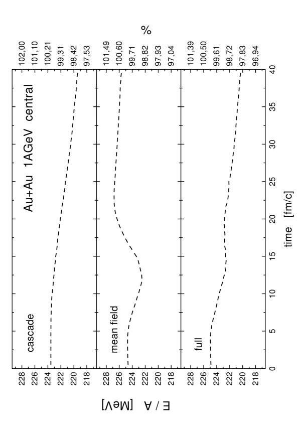
Figure 1:

Figure 2:

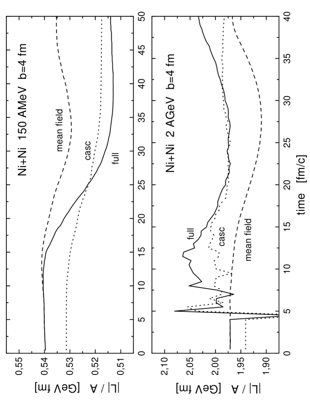
Figure 3:

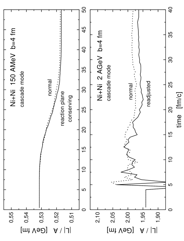
Figure 4:

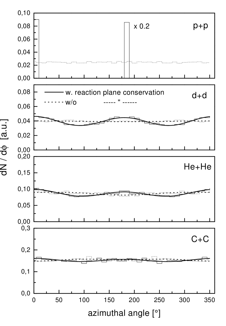
Figure 5:

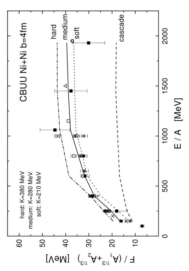
Figure 6:

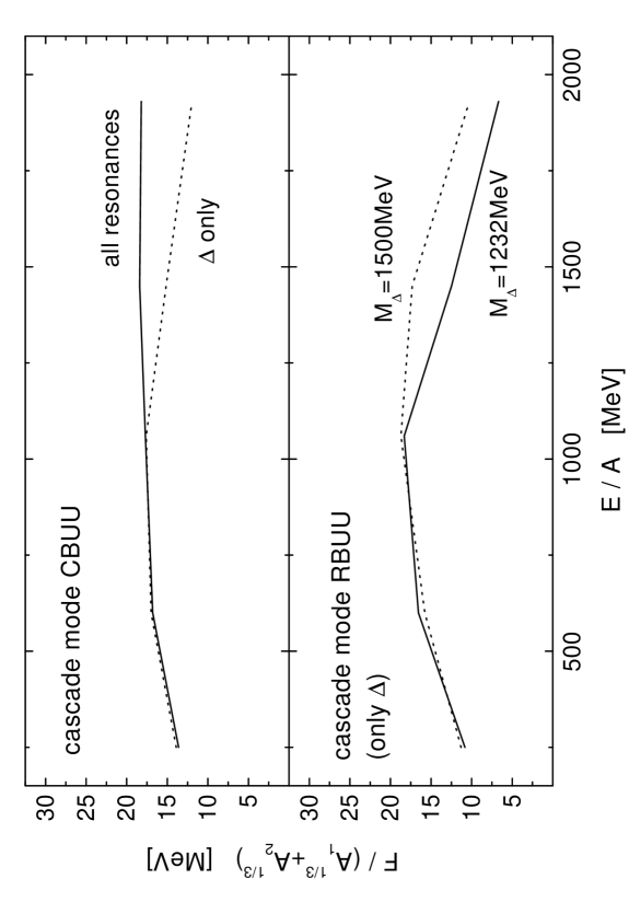
Figure 7:

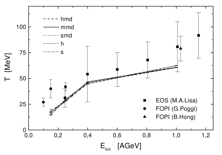
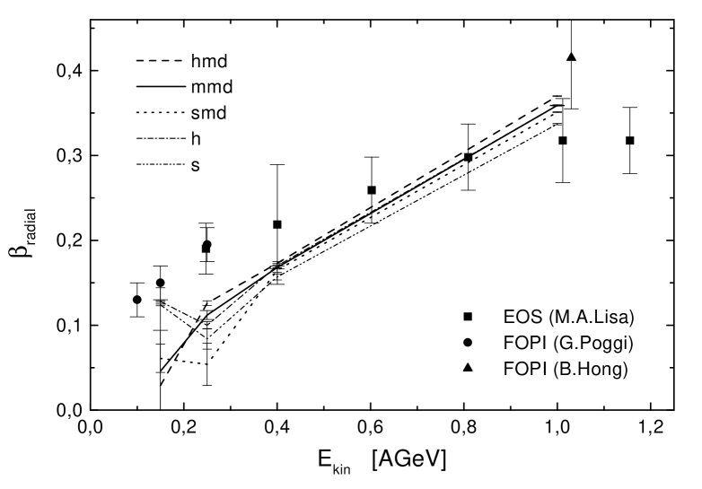
Figure 8:

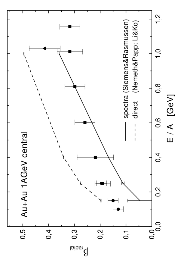
Figure 9:

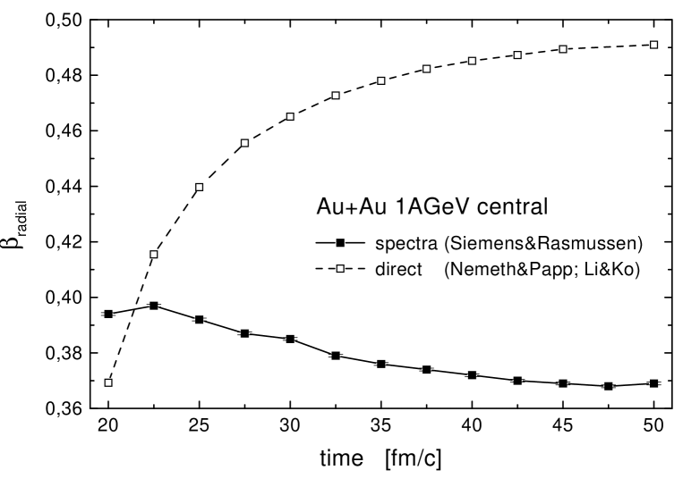
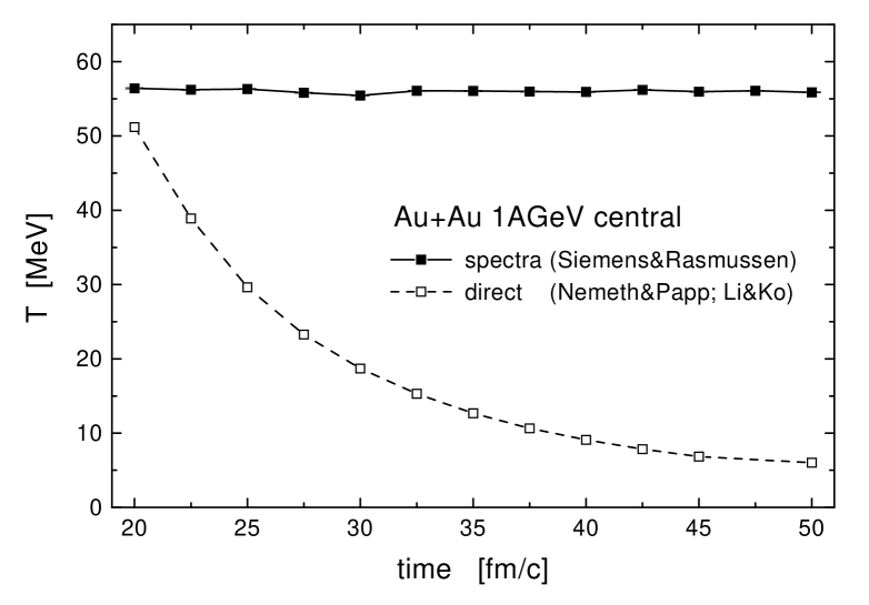
Figure 10:

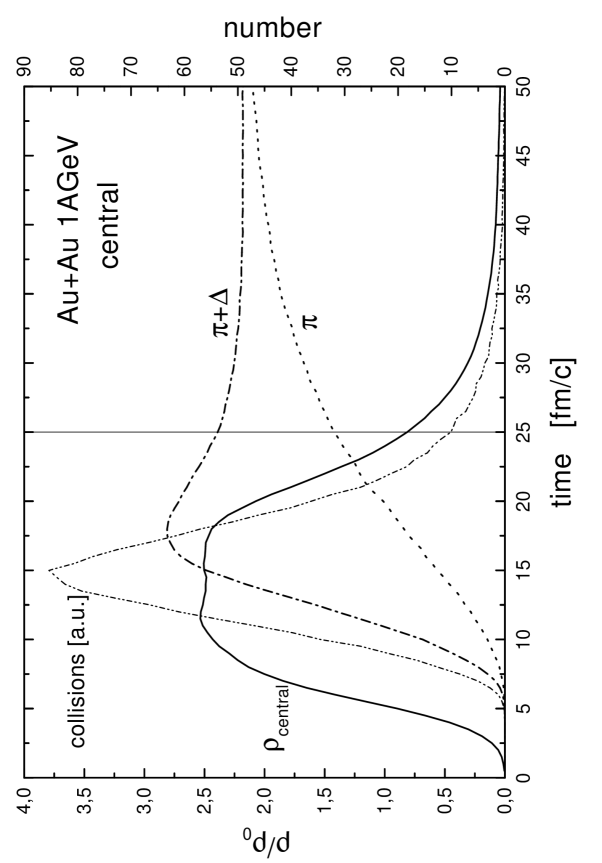
Figure 11:

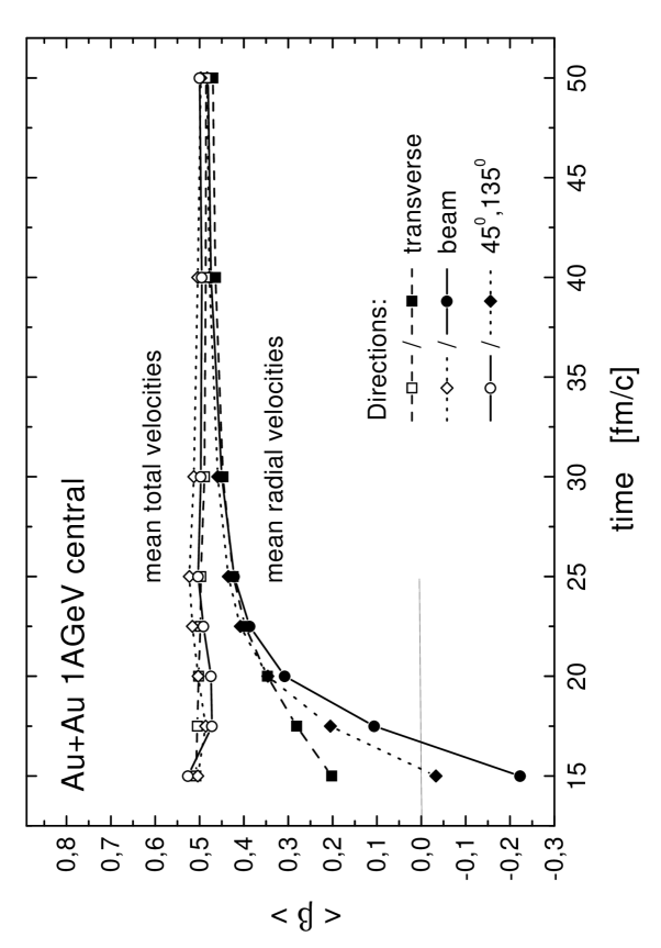
Figure 12:

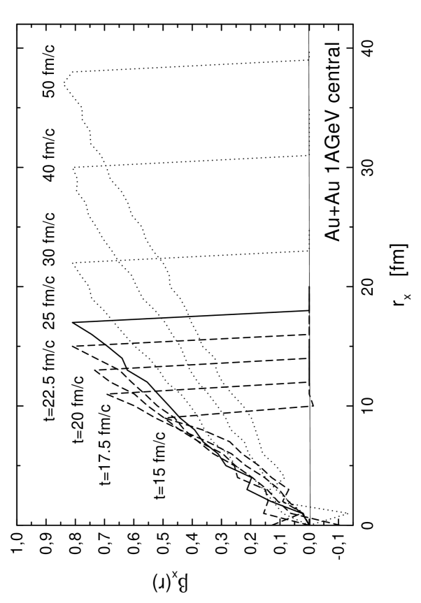
Figure 13:

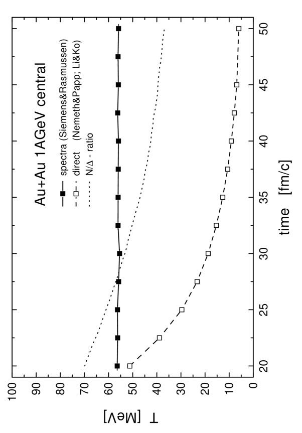
Figure 14:

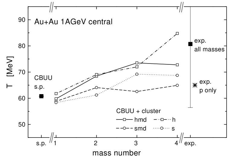
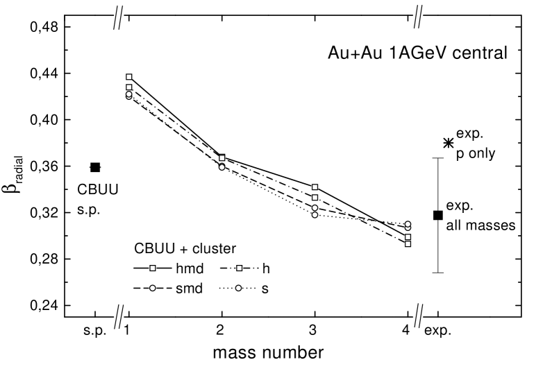
Figure 15:

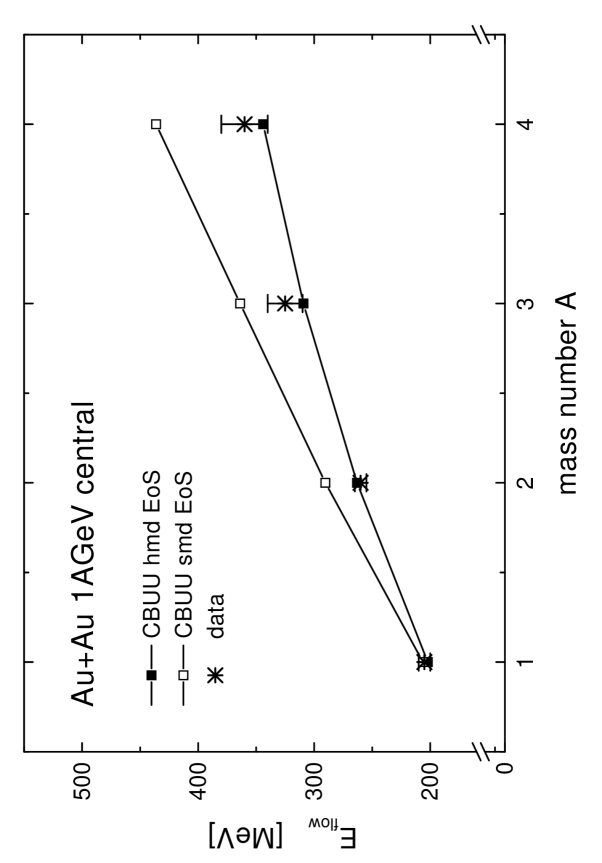
Figure 16:

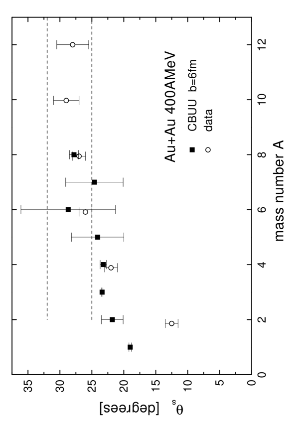
Figure 17:

References

- [1] C. Gale, G. Bertsch and S. Das Gupta, Phys. Rev. C35, 5 (1987) 1666.
- [2] G.M. Welke, M. Prakash, T.T.S. Kuo and S. Das Gupta, Phys. Rev. C38 (1988) 2101.
- [3] C. Gale, G.M. Welke, M. Prakash, S.J. Lee and S. Das Gupta, Phys. Rev. C41 (1990) 1545.
- [4] J. Zhang, S. Das Gupta and C. Gale, Phys. Rev. C50 (1994) 1617.
- [5] C. Roy et al., Z. Phys. A358 (1997) 73.
- [6] Q. Pan and P. Danielewicz, Phys. Rev. Lett. 70 (1993) 2062.
- [7] S. Bass et al., Prog. Part. Nucl. Phys. 41 (1998) 225.
- [8] Ch. Hartnack, R.K. Puri, J. Aichelin, J. Konopka, S.A. Bass, H. Stöcker and W. Greiner, Eur. Phys. J. A1 (1998) 151.
- [9] V. Ramilien et al., Nucl. Phys. A587 (1995) 802.
- [10] A. Lang, B. Blättel, V. Koch, K. Weber, W. Cassing and U. Mosel, Phys. Lett. B245 (1990) 147.
- [11] B. Blättel, V. Koch, A. Lang, K. Weber, W. Cassing and U. Mosel, Phys. Rev. C43 (1991) 2728.
- [12] S. Teis, W. Cassing, M. Effenberger, A. Hombach, U. Mosel and Gy. Wolf, Z. Phys. A356 (1997) 421.
- [13] M. Effenberger, A. Hombach, S. Teis and U. Mosel, Nucl. Phys. A614 (1997) 501.
- [14] M. Effenberger, A. Hombach, S. Teis and U. Mosel, Nucl. Phys. A613 (1997) 353.
- [15] Th. Weidmann, E.L. Bratkovskaya, W. Cassing and U. Mosel, nucl-th/9711004, Phys. Rev. C, in press.
- [16] A. Hombach, W. Cassing and U. Mosel, nucl-th/9809058, submitted to Eur. Phys. J. A.
- [17] Y. Leifels et al., GSI-Report 1/98 (1998) 57.
- [18] G.F. Bertsch and S. Das Gupta, Phys. Rep. 160 (1988) 189.
- [19] W. Cassing, K. Niita and S.J. Wang, Z. Phys. A331 (1988) 439.
- [20] W. Cassing, V. Metag, U. Mosel and K. Niita, Phys. Rep. 188 (1990) 363.
- [21] K. Weber, B. Blättel, W. Cassing, H.-C. Dönges, A. Lang, T. Maruyama and U. Mosel, Nucl. Phys. A552 (1993) 571.
- [22] W. Cassing and E.L. Bratkovskaya, Phys. Rep. 308 (1999) 65.
- [23] Review of Particle Properties, Phys. Rev. D50 (1994).
- [24] S. Teis, PhD Thesis, Giessen 1996.
- [25] V. Dimitriev and O. Sushkov, Nucl. Phys. A459(1986) 503.
- [26] S. Huber and J. Aichelin, Nucl. Phys. A573 (1994) 587.
- [27] L.G. Arnold and B.C. Clark, Phys. Rev. C19 (1979) 917.
- [28] T. Maruyama, W. Cassing, U. Mosel, S. Teis and K. Weber, Nucl. Phys. A573 (1994) 653.
- [29] C. Gale and S. Das Gupta, Phys. Rev. C42 4 (1990) 1577.
- [30] R.B. Wiringa, V. Fiks and A. Fabrocini, Phys. Rev. C38 (1988) 1010.
- [31] R.B. Wiringa, Phys. Rev. C38 (1988) 2967.
- [32] J. Stoer and R. Burlirsch, Vol. 1, Springer-Verlag, Berlin, (1978).
- [33] S. Teis, W. Cassing, M. Effenberger, A. Hombach, U. Mosel and Gy. Wolf, Z. Phys. A359 (1997) 297.
- [34] V. Metag, Nucl. Phys. A638 (1998) 45c.
- [35] P. Crochet et al., Nucl. Phys. A627 (1997) 522.
- [36] D.E. Kahana, D. Keane, Y. Pang, T. Schlagel and S. Wang, Phys. Rev. Lett. 74 (1995) 4404.
- [37] T. Kodama et al., Phys. Rev. C29 (1984) 2146.
- [38] N. Herrmann, Nucl. Phys. A610 (1996) 49c.
- [39] P.K. Sahu, A. Hombach, W. Cassing, M. Effenberger and U. Mosel, Nucl. Phys. A640 (1998) 493.
- [40] S. Hama, B.C. Clark, E.D. Cooper, H.S. Sherif and R.L. Mercer, Phys. Rev. C41 (1990) 2737.
- [41] B. Blättel, V. Koch, K. Weber, W. Cassing and U. Mosel, Nucl. Phys. A495 (1989) 381c.
- [42] C.M. Ko, Q. Li and R. Wang, Phys. Rev. C39 (1987) 1084.
- [43] B. Blättel, V. Koch and U. Mosel, Rep. Prog. Phys. 56 (1993) 1.
- [44] K. Weber, B. Blättel, W. Cassing, H.-C. Dönges, V. Koch, A. Lang and U. Mosel, Nucl. Phys. A539 (1992) 713.
- [45] S.C. Jeong et al., Phys. Rev. Lett. 72 (1994) 3468.
- [46] P.J. Siemens and J.O. Rasmussen, Phys. Rev. Lett. 42 (1979) 880.
- [47] M.A. Lisa et al., Phys. Rev. Lett. 75 (1995) 2662.
- [48] G. Poggi et al., Nucl. Phys. A586 (1995) 755.
- [49] B. Hong et al., Phys. Lett. B407 (1997) 115.
- [50] B.-A. Li and C.M. Ko, Nucl. Phys. A630 (1998) 556.
- [51] J. Nemeth and G. Papp, nucl-th/9711039.
- [52] V. Koch, B. Blättel, W. Cassing, U. Mosel and K. Weber, Phys. Lett. B241 (1991) 174.
- [53] K. Weber, B. Blättel, W. Cassing and U. Mosel, Nucl. Phys. A532 (1991) 715.
- [54] K.H. Kampert, J. Phys. G15 (1989) 691.
- [55] H.H. Gutbrod, A.M. Poskanzer and H.G. Ritter, Rep. Prog. Phys. 52 (1989) 1267.
- [56] H.G. Ritter et al., LBL-35590 (1994).
- [57] M.D. Partlan et al., Phys. Rev. Lett. 75 (1995) 2100.
- [58] W. Reisdorf and H.G. Ritter, Ann. Rev. Nucl. Part. Sci. 47 (1997) 1.