Shell Model Monte Carlo Investigation of Rare Earth Nuclei

Abstract

We utilize the Shell Model Monte Carlo (SMMC) method to study the structure of rare earth nuclei. This work demonstrates the first systematic “full oscillator shell plus intruder” calculations in such heavy nuclei. Exact solutions of a pairing plus quadrupole hamiltonian are compared with mean field and SPA approximations in several Dysprosium isotopes from $A=152-162$, including the odd mass $A=153$. Basic properties of these nuclei at various temperatures and spin are explored. These include energy, deformation, moments of inertia, pairing channel strengths, band crossing, and evolution of shell model occupation numbers. Exact level densities are also calculated and, in the case of ¹⁶²Dy, compared with experimental data.

I Introduction

Our goal is to develop an improved microscopic understanding of the structure of rare earth nuclei; i.e., an understanding based on the behavior of individual nucleons in the nucleus. Toward that end we solve the shell model systematically in a full oscillator shell basis with intruders for the first time in rare earth nuclei using the Monte Carlo (SMMC) technique; calculations using other methods have been restricted to a severely truncated model space. SMMC allows us to trace structural rearrangements within nuclei induced by changes in temperature and spin, so that we may obtain a clearer microscopic picture of general structural features in this region of the periodic table.

We assume an effective two-body nucleon-nucleon interaction and perform a Hubbard-Stratonovich transformation to obtain a path integral representation for the partition function, which is then evaluated by Monte Carlo methods (see Section II) to produce an exact shell model solution within statistical errors; this substantially enhances the predictive power of the nuclear shell model for some observables. Indeed, direct diagonalizations of the shell model Hamiltonian in a full basis have been limited to A$\sim 50$, while we present calculations for A$\sim 150$.

We examine how the phenomenologically motivated “pairing plus quadrupole” interaction compares in exact shell model solutions vs. the mean field treatment. We also examine how the shell model solutions compare with experimental data; static path approximation (SPA) calculations are also shown. There have been efforts recently by others to use SPA calculations, since it is simpler and faster (see [1, 2] as examples). However, the SPA results are not consistently good. In particular, it is useful to know not only if phenomenological pairing plus quadrupole type interactions can be used in exact solutions for large model spaces, but also if the parameters require significant renormalization because this affects the accuracy of the SPA.

We study a range of Dysprosium isotopes (Z=66, $86\leq N\leq 96$), which exhibit a rich spectrum of the behaviors such as shape transitions, level crossings, and pair transfer that have been observed in the rare earths. These results should therefore apply quite generally in the rare earth region, although the immediate work focuses on Dysprosium. We have selected this element since the half-filled proton shell makes the model spaces particularly large.

A previous paper discussed SMMC for the test case ¹⁷⁰Dy, which does not exist as a stable nucleus [3]. The work presented here is much more systematic and thorough. Algorithm improvements subsequent to  [3] have increased the computational execution by a factor of 10 or more and have allowed us to calculate the rare earths at lower temperatures, nuclear shapes are calculated using the correct calculated quadrupole variance (not just a constant), and pairing operators not used in  [3] are calculated.

II Theoretical background

Shell model diagonalization is still limited to $A\sim 50$ in the 0f1p shell [4]. In contrast, SMMC determines thermal observables, but explicit wave functions are never constructed; this is the key to how the predictive power of the shell model is extended so tremendously. The method is far less demanding on machine storage and there is no need to perform manipulations with the exponentially increasing numbers of variables that are encountered in direct diagonalization. SMMC storage scales like $N_{s}^{2}N_{t}$, where $N_{s}$ is the number of single particle shell model states and $N_{t}$ is the number of time slices (see below).

No known discrepancies exist between SMMC and direct diagonalization in cases where the comparison has been possible. This includes odd mass nuclei computed for appropriate temperatures. Realistic fp and sd-shell solutions using modified KB3 and Brown-Wildenthal interactions, respectively, agree with experiments [5]. These results give us a high degree of confidence in the SMMC technique.

As with any shell model, an effective nucleon-nucleon interaction must be specified. We use the well-known pairing plus quadrupole interaction as formulated by Kumar and Baranger [6]. The Hamiltonian is

$$\hat{H}=\hat{H}_{sp}-G_{p}\hat{P}_{p}^{\dagger}\hat{P}_{p}-G_{n}\hat{P}_{n}^{\dagger}\hat{P}_{n}-\frac{\chi}{2}\hat{Q}\cdot\hat{Q}$$ (1)

with $\hat{Q}=\hat{Q}_{p}+\hat{Q}_{n}$. The pairing and quadrupole operators are defined as

$$\hat{P}^{\dagger}_{J=0} = \sum_{jm}(-)^{j-m+l}\hat{a}^{\dagger}_{jm}\hat{a}^{\dagger}_{j-m}$$ (2)

$$\hat{Q}\cdot\hat{Q} = \sum_{i,j,k,l}\langle i|Q_{\mu}|k\rangle\langle l|Q_{\mu}|j\rangle\hat{a}^{\dagger}_{i}\hat{a}^{\dagger}_{j}\hat{a}_{l}\hat{a}_{k},$$ (3)

where $Q_{\mu}=r^{2}Y_{2\mu}(\theta,\phi)$ as usual. The single particle energies are also taken from Kumar and Baranger [6].

Effective charges are incorporated to account for core polarization to fit measured electric quadrupole transition strengths. The electric quadrupole operator, with effective charges $e_{p}$ and $e_{n}$, is

$$\hat{Q}=e_{p}\hat{Q}_{p}+e_{n}\hat{Q}_{n}$$ (4)

A Method and sign problem

Detailed procedures for the SMMC are explained fully in [5] and references therein. We provide no further explanation, except as regards the “sign problem.”

We define $\Phi\equiv$Tr$\hat{U}_{\sigma}/|$Tr$\hat{U}_{\sigma}|$ as the sign for a given Monte Carlo sample, where $\hat{U}_{\sigma}$ is defined as

$$\hat{U}_{\sigma} = \hat{U}_{N_{t}}\hat{U}_{N_{t}-1}...\hat{U}_{1}$$ (5)

$$\hat{U}_{n} = e^{-\Delta\beta\hat{h}_{\sigma}}$$ (6)

$\hat{h}_{\sigma}$ is the one body hamiltonian for the auxiliary field configuration $\sigma$ and $\beta$ is the inverse temperature. In SMMC, the partition function path integral is divided into $N_{t}$ time steps of size $\Delta\beta$ so that $\beta=N_{t}\Delta\beta$. Hence, the complete evolution operator is expressed as a product of operators in each time step. In these studies, we use the canonical (number projection) formalism to evaluate the trace.

If $\Phi$ is not equal to one, numerical instabilities can arise. This has become widely known as the Monte Carlo “sign problem.” The simple phenomenological pairing plus quadrupole interaction (without added pn pairing) does not have an inherent sign problem. However, sign problems can arise even with this simple interaction if time reversal symmetry is broken, as when odd masses are studied or the system is cranked by adding a term $-\omega\hat{J}_{z}$ to $\hat{H}$. In these studies, the sign violation turned out to be minor for odd mass ground states and canonical ensemble cranking was limited to $\omega\leq 0.3$ MeV. Experimentally, these nuclei are observed to $\omega\approx 0.6$ MeV [7].

B Shapes and moments of inertia

The quadrupole expectation values $\langle Q_{\mu}\rangle$ vanish under rotational symmetry. However, for a given Monte Carlo sample $Q_{\mu}$ will have some finite, nozero value. We calculate $Q_{ij}=3x_{i}x_{j}-\delta_{ij}r^{2}$ for each sample and relate its eigenvalues to the quadrupole $\beta$ and $\gamma$ deformation parameters as done previously with SMMC [8, 3]. The intrinsic frame for each sample with a field configuration $\sigma$ has nonzero components $Q^{\prime}_{0}$ and $Q^{\prime}_{2}=Q^{\prime}_{-2}$ as

$$\langle Q_{0}^{\prime}\rangle_{\sigma} = \frac{3}{2\pi}\sqrt{\frac{4\pi}{5}}\langle r^{2}\rangle_{\sigma}\beta_{\sigma}\cos\gamma_{\sigma}$$ (8)

$$\langle Q_{2}^{\prime}\rangle_{\sigma} = \frac{3}{2\pi}\sqrt{\frac{4\pi}{5}}\langle r^{2}\rangle_{\sigma}\frac{\beta_{\sigma}}{\sqrt{2}}\sin\gamma_{\sigma}$$ (9)

In terms of eigenvalues $Q^{\prime}_{11},Q^{\prime}_{22}$, and $Q^{\prime}_{33}$ of $Q_{ij}$ give

$$\langle Q_{11}^{\prime}\rangle_{\sigma} = \sqrt{\frac{2\pi}{5}}\left(\sqrt{3}(\langle Q_{2}^{\prime}\rangle_{\sigma}+\langle Q_{-2}^{\prime}\rangle_{\sigma})-\sqrt{2}\langle Q_{0}^{\prime}\rangle_{\sigma}\right)$$ (10)

$$\langle Q_{22}^{\prime}\rangle_{\sigma} = \sqrt{\frac{2\pi}{5}}\left(-\sqrt{3}(\langle Q_{2}^{\prime}\rangle_{\sigma}+\langle Q_{-2}^{\prime}\rangle_{\sigma})-\sqrt{2}\langle Q_{0}^{\prime}\rangle_{\sigma}\right)$$ (11)

$$\langle Q_{33}^{\prime}\rangle_{\sigma} = 2\sqrt{\frac{4\pi}{5}}\langle Q_{0}^{\prime}\rangle_{\sigma}$$ (12)

We can also calculate the free energy $F(\beta,\gamma)$ to construct shape contour plots. This is done using

$$F(\beta,\gamma)=-T\ln{\frac{P(\beta,\gamma)}{\beta^{3}\sin{3\gamma}}}$$ (13)

$P(\beta,\gamma)$ is the shape distribution as a function of the deformation coordinates $(\beta,\gamma)$ and $T$ is the temperature. Plots are truncated at small $\gamma$ for an obvious reason. All shape plots discussed in this paper are for the mass quadrupole and are not electric quadrupole.

Moments of inertia are calculated in the cranked Hamiltonian ($\hat{H}\rightarrow\hat{H}-\omega\hat{J}_{z}$) using ${\cal I}_{2}=d\langle\hat{J}_{z}\rangle/d\omega$. We expect moments of inertia to initially increase as the nucleus is cranked and then to decrease when pairs are broken.

C Pairing composition

Pairing correlations in nuclei can be studied by calculating pairing strengths in different spins for protons and neutrons. For like particle pairs, define the pair creation operator as

$$A^{\dagger}_{JM}=\frac{1}{\sqrt{1+\delta_{ab}}}[\hat{a}^{\dagger}_{j_{a}}\times\hat{a}^{\dagger}_{j_{b}}]_{JM}(-)^{l_{b}}$$ (14)

where

$$[\hat{a}^{\dagger}_{j_{a}}\times\hat{a}^{\dagger}_{j_{b}}]_{JM}=\sum_{m_{a},m_{b}}(j_{a}m_{a}j_{b}m_{b}|JM)\hat{a}^{\dagger}_{j_{a}}\hat{a}^{\dagger}_{j_{b}}$$ (15)

Note that we only consider like particle pairing, i.e., proton-proton and neutron-neutron (Eq. 1). Now let $\alpha=(j_{a},j_{b})$ and $\alpha^{\prime}=(j_{c},j_{d})$. Using the pair creation operator, a matrix $M^{J}_{\alpha,\alpha^{\prime}}$ can be constructed as

$$M^{J\pi}_{\alpha,\alpha^{\prime}}=\sum_{M}\langle A^{\dagger}_{JM}(j_{a},j_{b})A_{JM}(j_{c},j_{d})\rangle$$ (16)

from which we can then define a pairing strength $P^{J}$ as

$$P^{J\pi}=\sum_{\alpha\geq\alpha^{\prime}}M^{J\pi}_{\alpha,\alpha^{\prime}}$$ (17)

The correlated pair strength, which is more useful, is obtained by subtracting uncorrelated mean field pairs from the total $P^{J\pi}$ defined above. A Fermi gas has generally been used for the mean field with SMMC. Letting $n_{k}=\langle\hat{a}^{\dagger}_{k}\hat{a}_{k}\rangle$ and substituting $n_{1}n_{2}(\delta_{13}\delta_{24}-\delta_{23}\delta_{14})$ for $\langle\hat{a}^{\dagger}_{1}\hat{a}^{\dagger}_{2}a_{3}a_{4}\rangle$ in Eq. 16 yields the Fermi gas mean field pair strength $P^{J\pi}_{MF}$. In this case, of course, we could use the SPA occupations as the “mean field” to subtract from the complete pairing plus quadrupole solutions.

Even-even nuclei have correlated ground states, so we expect an excess of $J~{}=~{}0$ pairs beyond the mean field in even-even ground states. The hallmark for a pair condensate is the existence of one eigenvalue of $M^{J\pi}_{\alpha,\alpha^{\prime}}$ which is much greater than all the rest.

The pair matrix can be diagonalized to find the eigenbosons $B^{\dagger}_{\alpha JM\pi}$ as

$$B^{\dagger}_{\alpha JM\pi}=\sum_{ab}\psi_{\alpha JM\pi}(ab)A^{\dagger}_{JM\pi}(ab)\;,$$ (18)

where $\alpha=1,2,\cdots$ labels the various bosons with the same angular momentum and parity. The $\psi_{\alpha J\pi}$ are the eigenvectors of the diagonalization, i.e. the wavefunctions of the boson, and satisfy the relation

$$\sum_{j_{a}j_{b}}\psi^{*}_{\alpha J\pi}\psi_{\mu J\pi}=\delta_{\alpha\mu}\;.$$ (19)

These eigenbosons satisfy

$$\sum_{M}\langle B_{\alpha JM\pi}^{\dagger}B_{\gamma JM\pi}\rangle=n_{\alpha J\pi}\delta_{\alpha\gamma}\;,$$ (20)

where the positive eigenvalues $n_{\alpha J\pi}$ are the number of $J\pi$-pairs of type $\alpha$.

D Backbending

We can monitor the pair strength for neutrons coupled to $J=12$ as a signature for the anticipated band crossing or backbending. The only orbital in our model space which can produce this coupling is the neutron $i_{13/2}$ level. We do not monitor backbending by mapping out the typical backbending plot of $I$ vs. $\omega$ because the backbend in the plot requires a multivalued solution of $I$, whereas SMMC always produces a single-valued solution from the statistical ensemble.

E Level density in SMMC

SMMC is an excellent way to calculate level densities. $E(\beta)=\langle\hat{H}\rangle$ is calculated for many values of $\beta$ which then determine the partition function, $Z$, as

$$\ln[Z(\beta)/Z(0)]=-\int_{0}^{\beta}d\beta^{\prime}E(\beta^{\prime});$$ (21)

$Z(0)$ is the total number of available states in the space. The level density is then computed as an inverse Laplace transform of $Z$. Here, the last step is performed with a saddle point approximation:

$$S(E) = \beta E+\ln Z(\beta)$$ (22)

$$\rho(E) = (2\pi\beta^{-2}C)^{-1/2}\exp(S),$$ (23)

where $\beta^{-2}C\equiv-dE/d\beta$. SMMC has been used recently to calculate level densities in iron region nuclei [9]. Here, we present the first exact level density calculation for the much heavier Dy.

Nuclear level densities in the static path approximation has previously been investigated by Alhassid and Bush for a simple solvable Lipkin model [10]. The simple Lipkin Hamiltonian does not include pairing, however. These authors found SPA to be superior to the mean field approximation and the difference between the two depended on interaction strength.

F Recap on interaction and model space

It is fortunate that the elementary pairing plus quadrupole interaction does not break the Monte Carlo sign so that no g-extrapolation is required. The calculation of level densities is also simplified, since accurate results require very low statistical uncertainties [9].

We do not include isovector proton-neutron (pn) pairing in the interaction. This is a reasonable assumption since fp shell calculations with SMMC have shown clearly that isovector pn correlations diminish quickly as N exceeds Z and we are not at N$\sim$Z [11]. Further, in our case the valence protons and neutrons occupy different oscillator shells. To be sure some pn correlations are included via the isoscalar quadrupole interaction ($2\hat{Q}_{p}\cdot\hat{Q}_{n}$), but any observable that depends strongly on pn correlations such as the Gamow-Teller strength will not be accurately determined with this interaction.

We choose one shell each for protons (sdg) and neutrons (pfh) with the opposite parity intruders $h_{11/2}$ and $i_{13/2}$, respectively. The space encompasses $32$ proton levels and $44$ neutron levels. The oscillator length, $b=\sqrt{\hbar/m\omega_{0}}$, was taken to be $1.01A^{1/6}$ fm.

With this space, Dy has sixteen valence protons so that the proton shell is half-filled. The number of valence neutrons varies from four in ¹⁵²Dy to fourteen in ¹⁶²Dy. This model space is identical to the one used by Kisslinger and Sorensen [12], but is smaller than the two shell space Kumar and Baranger used.

G Static path approximation and mean field

The static path approximation (SPA) is the one-time-slice limit of the partition function path integral and is obviously easily implemented in SMMC. The mean field approximation is the saddle point estimation of the path integral; neither includes imaginary time-dependent terms. The SPA differs from mean field since the integral over time-independent auxiliary fields in SPA is done exactly, so that contributions from multiple configurations (even with large fluctuations) are included rather than just the single, steepest-descent mean field.

Static path calculations do not do as well with realistic interactions as with schematic interactions, e.g., pairing plus quadrupole. Also, the accuracy of the approximation varies among operators, as will be demonstrated in Section III.

Static path calculations were done in SMMC with continuous fields rather than the discrete field sampling that has typically been used with SMMC. However, continuous sampling is not used for other calculations due to the significantly increased number of thermalization cycles it would require. Continuous fields proved necessary for accurate results in SPA; calculated energies were higher for discretized fields than for continuous fields and the difference could not be attributed to statistical uncertainties.

III Results

A SPA vs. full solution: static properties

1 Energy, spin, and quadrupole moments

Comparisons of SPA and full path solutions for the static observables energy $\langle H\rangle$, spin $\langle J^{2}\rangle$, and mass quadrupole moment $\langle Q^{2}\rangle$ are shown for the experimentally deformed, transitional, and spherical isotopes in Figs. 1(a)-(i). A few of the full canonical calculations do not extend quite as low in temperature as the SPA results due to numerical instability developing from multiple matrix multiplications. Error bars in these plots are smaller than the dot sizes and are therefore not shown. Also, note that the quadrupole moments are expressed as $\langle Q^{2}\rangle/b^{4}$, where $b$ is the oscillator length.

The SPA energy is greater than the exact energy, except at very high temperatures for all three of these nuclei; at the lowest temperatures, the difference is a few MeV. The origin of this discrepancy will be discussed below (Section III A 2). The difference between SPA and exact canonical ground state energies is $2.39\pm 0.15$ MeV for ¹⁵²Dy and $2.59\pm 0.18$ MeV for ¹⁵⁶Dy, so there is not a significant discrepancy between the lighter and heavier isotopes. Thus, SPA does not predict absolute energies accurately, but works well for relative differences. The partition function integral in SMMC is always divided into time steps of fixed size $\Delta\beta$, which is fixed at 0.0625 MeV^-1. As the temperature, $1/\beta$, increases the number of time slices in the exact partition function expression decreases. Hence, it is not surprising that SPA is more accurate for higher temperatures.

Looking at $\langle J^{2}\rangle$ shows that the SPA calculations only cool to about $J=8-10$ for even the lowest calculated temperatures while the even-even ground states are of course $J=0$. In these canonical SMMC calculations, $J=0$ is not exactly reached even in the full canonical calculations because the thermal ensemble always includes contributions from higher energy states. An estimate for the $\beta$ required for good filtering to the even-even ground states is $\beta=1/E(2_{1}^{+})$, where $E(2_{1}^{+})$ is the measured energy of the first $2^{+}$ state. This $\beta$ value varies from $\beta=1.6$ MeV^-1 for ¹⁵²Dy to $\beta=11.5$ MeV^-1 for ¹⁶²Dy as $E(2_{1}^{+})$ varies from 0.614 to 0.087 MeV.

The thermal spin expectation, $\langle J^{2}\rangle$, can, in principle, be compared against the experimental spectra. However, one never experimentally knows all the states in a nucleus so such a direct comparison is difficult except at low excitation energies which are dominated by the well known ground state band. The difference in $\langle J^{2}\rangle$ between SPA and full canonical solutions at the lowest temperatures is $58$ for ¹⁵²Dy, $74$ for ¹⁵⁴Dy, and $91$ for ¹⁵⁶Dy. Hence, the deviation is worse with increasing deformation in these isotopes.

SPA works very well for the quadrupole moments. This result is also very robust, i.e., strengthening or weakening the coupling $\chi$ beyond the nominal Kumar-Baranger value does affect the agreement between SPA and exact results.

More information about the static quadrupole moment appears in Figs. 2(a)-(d), where the proton and neutron quadrupole components are shown separately. The neutron quadrupole moment increases quickly from ¹⁵²Dy to ¹⁵⁴Dy and increases much more slowly after the onset of deformation in ¹⁵⁶Dy. The proton quadrupole moment, meanwhile, remains approximately fixed for all the studied isotopes. $\langle Q^{2}_{v}\rangle$ increases rapidly as $A$ increases from $154$ to $162$. Relative to $\langle Q^{2}\rangle$ it is only 8.5% (Fig. 2(a)), but the total quadrupole moment at $\beta=6$ MeV^-1 is 46% larger for ¹⁶²Dy than for ¹⁵⁶Dy ($1221\;b^{4}$ vs. $834\;b^{4}$). $\langle Q^{2}_{v}\rangle/\langle Q^{2}\rangle$ is roughly 10% for all isotopes, where $Q_{v}$ is the isovector quadrupole operator ($Q_{p}-Q_{n}$).

Another comparison between SPA and full canonical calculations is how quickly the solutions cool for various observables. For example, in ¹⁵²Dy $\langle H\rangle$ appears to have stabilized by $\beta=6$ MeV^-1 in both SPA and the full solution. The spin $\langle J^{2}\rangle$ and quadrupole moment $\langle Q^{2}\rangle$ also appear to have minimized near $\beta=6$ MeV^-1 in the SPA and exact calculations. Similar results are evident in the other nuclei, except for $\langle J^{2}\rangle$ in ¹⁵⁶Dy which is clearly decreasing still in SPA for $\beta=8$ MeV^-1, the largest value for which the calculation could be done.

2 Pairing energy and gaps

Some insight can be had by looking at the pairing energy and gaps. The quadrupole energy,$-0.5\chi\langle\hat{Q}\cdot\hat{Q}\rangle$ in SPA agrees well with the full canonical solution, but the total energies in SPA shown above have clear deviations from the exact canonical results. The difference in $\langle H\rangle$ is due to the pairing energy. The accuracy of the SPA in the pairing interaction depends strongly on the pairing strength and is naturally better for weaker pairing.

The pairing energies and BCS pair gaps for ^152-156Dy are shown in Figs. 3(a)-(f). The latter were obtained from the pairing energies by $\Delta^{2}_{BCS}/G=H_{pair}$. The disagreement between SPA and exact calculations looks worse for protons, but recall that there are 16 valence protons and just 4-8 valence neutrons in these isotopes.

B B(E2) and effective charges

The reduced electric quadrupole transition strength, $B(E2)$, is computed from

$$B(E2)=\langle(e_{p}\hat{Q}_{p}+e_{n}\hat{Q}_{n})^{2}\rangle$$ (24)

where $e_{p}$ and $e_{n}$ are effective proton and neutron charges. We have taken $e_{p}=1+x,e_{n}=x$. Results are shown in Table I and Fig. 4, where it has been assumed that the total $B(E2)$ calculated in SMMC is the same as $B(E2;2_{1}^{+}\rightarrow 0_{1}^{+})$. Effective charges in column 3 and column 4 are fitted to measured $B(E2)$ values. Typical effective charges in rare earths are approximately $e_{p(n)}=2(1)$, so these values are in a reasonable range.

Table I and Fig. 4 also show what $B(E2)$ strength would be obtained from SMMC quadrupole moments with Kumar-Baranger charges. This illustrates how a small change in the effective charge can produce a comparatively large change in the $B(E2)$. For ¹⁶²Dy, the $7\%$ difference in $e_{p}$ when using Kumar-Baranger charges leads to a $23\%$ change in $B(E2)$.

The collectivity of a nucleus, and thus the $B(E2)$ value, varies with the energy $E(2_{1}^{+})$. The effective proton charge, $e_{p}$, is plotted against $E(2_{1}^{+})$ in Fig. 5. For the SMMC results, the neutron effective charge needs to be zero for spherical ¹⁵²Dy to avoid severely overestimating the $B(E2;2_{1}^{+}\rightarrow 0_{1}^{+})$ strength as it is calculated above. The fitted effective charge is $e_{p}=1.75$ for the deformed isotopes and it is intermediate for ¹⁵⁴Dy. This is a reflection of the fact that exact solutions for the mean field interaction yield lighter dysprosiums which are too deformed (Section III F); the effective charge should be constant.

It should be noted that Kumar and Baranger did not calculate $B(E2)$ values for spherical nuclei in the same way as for deformed nuclei, i.e., they did not take effective charges for spherical nuclei as $e_{p}=1+1.5Z/A$, $e_{n}=1.5Z/A$. For spherical nuclei, they combined phonon and rotational model properties (see [6] p. 552). They used $E(2_{1}^{+})=(C/B)^{1/2}$ and $B(E2,0\rightarrow 2)\propto Z^{2}R_{0}^{4}(BC)^{-1/2}$ from the phonon model with the relation $Q_{s}\propto B(E2)^{1/2}$. These $E(2_{1}^{+})$ predictions are not very good (Table II).

C SPA vs. full solution: cranking

D Sign limits on cranking

Recall from Section II A that cranking degrades the Monte Carlo sign from unity and that calculations become impractical when the sign drops below 0.5. This is illustrated for both full canonical and SPA results for ¹⁵⁶Dy in Figs. 6(a)-(b). Error bars are not displayed in these figures since they are small; the statistical error in $\Phi$ for $\beta=6$ MeV^-1 and $\omega=0.3$ MeV is 0.04. Canonical cranking in this nucleus is limited to small frequencies for $\beta=8$ MeV^-1, as evidenced by the quick drop in sign from $\omega=0.05$ MeV to $\omega=0.1$ MeV. The canonical cranking is fairly good for $\beta\leq 6$ MeV^-1, especially $\beta\leq 4$ MeV^-1. SPA cranking predictably has better sign properties. In SPA, ¹⁵⁶Dy can be cranked well out to $\beta=8$ MeV^-1, which is the approximate limit of temperature that can be reached in this nucleus without matrix stabilization.

1 Energy, spin, and quadrupole moments again

Energy, spin, and quadrupole moments at various temperatures are compared at different cranking frequencies in exact canonical and SPA. Calculations for ¹⁵⁶Dy appear in Figs. 7(a)-(f). Energy results for SPA at different cranking frequencies mirror the full canonical result. In the range $5\leq\beta\leq 8$ MeV^-1, or $0.2\leq T\leq 0.125$ MeV, $\omega=0.1$ MeV lies at small excitation energy $\epsilon$ above the $\omega=0$ baseline, $\omega=0.2$ MeV lies roughly $3\epsilon$ above the baseline, and $\omega=0.3$ MeV is excited by approximately $6\epsilon$ above $\omega=0$.

The spin results reveal that $\langle J^{2}\rangle$ in SPA is higher than the exact canonical result until $T\geq 1$ MeV when $\omega\leq 0.2$ MeV. However, for $\omega=0.3$ MeV, SPA agrees well with the exact solution. The exact solution is not shown for $\beta=8$ MeV^-1 at this frequency due to numerical difficulties. The SPA $\langle J^{2}\rangle$ for $\omega=0.2$ MeV is very flat across the computed temperature range, $0.125\leq T\leq 1$ MeV. As with the exact solution, $\langle J^{2}\rangle$ decreases with rising temperature for $\omega=0.3$ MeV.

Quadrupole results with cranking are similar to the $\omega=0$ results in that the quadrupole moment does not change when the temperature is decreased below 200 keV at any frequency studied here. Note that the quadrupole results are plotted vs. $\omega$ for various temperatures. At the lowest temperatures, the quadrupole moment begins to decrease after $\omega=0.15$ MeV in the canonical case. It decreases after $\omega=0.1$ MeV in the SPA, however, $\omega=0.15$ MeV is not computed there so it is difficult to say if the quadrupole moment is declining at frequency $0.1$ or $0.15$ MeV in SPA. SPA agrees very well with the exact solution for $\langle Q^{2}\rangle$ at all temperatures and cranking frequencies computed.

2 Moments of inertia

The $J_{z}$ variation with cranking frequency determines the moment of inertia. Results for ¹⁵⁶Dy are displayed in Figs. 8$(a)-(b)$ for both canonical and SPA cases.

The moment of inertia, ${\cal I}_{2}$, for ¹⁵⁶Dy is $44.6\pm 7$ $\hbar^{2}$/MeV in the exact canonical ensemble at $J\approx 4$ with $\beta=8$ MeV^-1 and is $73.0\pm 2$ $\hbar^{2}$/MeV at same $\omega$ in SPA. At this temperature, $T=0.125$ MeV, the SPA moment of inertia is $64\%$ larger than the exact result. The experimental moment of inertia ${\cal I}_{2}=40\hbar^{2}$/MeV at $J=4$, which matches the SMMC canonical result. Also, the rigid body moment of inertia for ¹⁵⁶Dy with $(\beta,\gamma)=(0.24,0)$ is $73\hbar^{2}$/MeV. This coincides with the SPA moment of inertia.

E Band crossing

The pairing strength for $J=12$ pairs in ¹⁵⁶Dy, which can be produced only from $i_{13/2}$ neutron pairs, is shown in Fig. 8(c)-(d). The strength $P_{J=12}$ begins to increase quickly in the canonical case for $(\beta,\omega)=(8,0.15)$, which corresponds to $J=16\pm 1$. In SPA, $P_{J=12}$ increases sharply beyond $(\beta,\omega)=(8,0.1)$, which corresponds to $J=14$.

The occupations of both the proton $h_{11/2}$ and neutron $i_{13/2}$ intruder orbitals for ¹⁵⁶Dy are given in Figs. 9(a)-(b). The proton intruder occupation is comparatively stable over this same spin range at each temperature. However, it is clear that the $i_{13/2}$ occupation is increasing with spin, particularly for lower temperatures, as expected. The $h_{11/2}$ occupation number decreases slightly with temperature for all frequencies computed. Occupation shifts slightly to $\pi d_{5/2}$. For $\beta=6$ MeV^-1, the maximum spin $J_{z}$ corresponds to $J\approx 32$ and for $\beta=1$ MeV^-1, the maximum spin is $J\approx 28$. Unfortunately for $\beta=6$ MeV^-1, or $T=167$ keV, the Monte Carlo sign is reduced to $0.4$ at the maximum spin shown (recall Fig. 6). At $\beta=1$ MeV^-1, however, the sign is still very stable at $0.96$.

F Shape vs. temperature and spin

Nuclear shapes have also been computed to clarify how the shape varies with temperature and spin. Temperatures and frequencies for these calculations are given in the figure captions. In all shape graphs, the $\beta$-axis is radial and the other axis is the $\gamma$-axis. Results for ¹⁵²Dy at temperatures from $T=0.25$ MeV to $T=2$ MeV are shown in Fig. 10. The nucleus becomes increasingly spherical for rising temperature.

Shapes for ¹⁵⁴ Dy and ¹⁵⁶Dy are shown in Figs. 11-13. These were all produced from the exact canonical ensemble except Fig. 12(f), which was produced with the static path approximation. Cranked contour plots, such as Fig. 13(d) for ¹⁵⁶Dy at $(\beta,\omega)=(8,0.1)$, show the nuclei becoming increasingly gamma-soft with increasing spin. This is also true in SPA (Fig. 12(f)), which was utilized in this case since the Monte Carlo sign for the exact calculation becomes too small to obtain useful results. There is no sign of oblate shape at this spin in ¹⁵⁴Dy, as predicted by Cranmer-Gordon, et al., using a Nilsson-Strutinsky cranking model [13]. However, the SMMC ground state deformation in ¹⁵⁴Dy with these parameters is clearly too large. Ma, et al. [14] claimed evidence for a return to some collectivity in ¹⁵⁴Dy from spin 36⁺-$48^{+}$. The shape plot for ¹⁵⁴Dy at $J\sim 50$ (Fig. 12(f)) appears soft. The SMMC $B(E2)=5$ W.U. at this spin using the fitted effective charge.

Note that with increasing A in these isotopes, the ground state deformation is roughly constant and the depth of the minimum increases. In fact for ¹⁵⁶Dy, the depth of the well is roughly the same as the fission barrier ($\sim 40$ MeV) [15]. However, it can be questioned whether our shape formalism (Eq. 13) should be applied at such low temperatures ($T\leq 0.25$ MeV) since in the limit $T\rightarrow 0$ the free energy becomes everywhere degenerate and zero. The very low temperature results for ¹⁵⁶Dy and ¹⁶²Dy (not shown) do not coincide with the mean field.

Previous publication of shape plots from SMMC results in gamma-soft nuclei using a pairing plus quadrupole Hamiltonian with quadrupole pairing [16] did not exhibit this. However, those nuclei are only weakly deformed ($\beta\approx 0.05-0.15$) while the Dysprosiums with A$\geq$154 are well-deformed ($\beta\approx 0.3$). For the Dysprosium shapes in this paper, the unexpected depth of the potential well is only evident for well-deformed cases.

It is apparent from the above that the dysprosiums are all deformed in their ground states in the exact model calculation. However, ¹⁵²Dy is known experimentally to be spherical. Kumar and Baranger did not calculate ¹⁵²Dy, though they did calculate some other spherical isotopes. A shape plot has also been constructed from SMMC results in ¹⁴⁰Ba for comparison with Kumar and Baranger (Fig. 14). The SMMC result for ¹⁴⁰Ba agrees with Kumar-Baranger; both calculations indeed show a spherical nucleus. This isotope has $Z=56$ and $N=84$. For the shell model space used, this becomes six valence protons and two valence neutrons so that, unlike dysprosium, the proton shell is less than half filled. The SMMC $B(E2;2\rightarrow 0)$ is $5$ W.U. using the effective charge fitted for the dysprosiums. Reducing the quadrupole coupling to half its mean field strength still yielded deformation $\beta\approx 0.3$ for ¹⁵⁶Dy with a deep potential. However, reducing $\chi$ to half the mean field strength returns ¹⁵²Dy to a spherical distribution which fits the measured $B(E2)$ strength with effective charges $(e_{p},e_{n})=(1,0)$.

The equilibrium shape was also calculated in ¹⁴⁴Ba for inverse temperature $\beta=4$ MeV^-1. ¹⁴⁴Ba has $E(2_{1}^{+})=199$ keV [23] and deformation $\beta=0.19$ [24]. This nucleus proved to be extremely deformed ($\beta\approx 0.45$) in SMMC with the Kumar-Baranger interaction parameters, but with a deformation well not nearly so deep as for the $A\geq 154$ Dysprosiums (Fig. 15). In this case, the potential was only about 2.5 MeV deep. Kumar and Baranger did not calculate this isotope, so direct comparison with them is not possible in this case. Kumar and Baranger also made no claims their model is valid for nuclei at such extreme deformation [22].

G Odd A

As mentioned previously, the odd nucleon in an odd mass nucleus violates T-reversal symmetry and can break the Monte Carlo sign, even with an interaction free from repulsive contributions. Results from ¹⁵³Dy are shown below in Figs. 16(a)-(e). In this case, for our simple Hamiltonian the Monte Carlo sign behaves well and remains at 0.82 for canonical $\beta=10$. Also, some of this reduction in sign may in fact be due to limits of numerical accuracy in the machine.

1 Static observables

Results for static observables are quantitatively similar to the even-even results. The energy difference between the full canonical and SPA calculations at $T=100$ keV is $1.97\pm 0.4$ MeV (Fig. 16(a)), which is a little less than the $2.49\pm 0.16$ MeV canonical-SPA energy difference in neighboring ¹⁵²Dy and the $2.15\pm 0.06$ difference in ¹⁵⁴Dy. This difference is due to different pairing energies in these odd-even and even-even isotopes. The discrepancy in $\langle J^{2}\rangle$ between SPA and full solutions is $\Delta J^{2}=66$ or $\Delta J\approx 8$ (Fig. 16(b)). The ground state spin for ¹⁵³Dy is $(7/2)^{-}$ so that $\langle J^{2}\rangle=15.75$ and the first excited state is $(3/2)^{-}$ at excitation $E=109$ keV. Thus, the estimated $\beta$ needed for filtering the ground state is reachable and $\langle J^{2}\rangle=16\pm 4$ in the SMMC canonical ensemble agrees very well with experiment. Again, the SPA quadrupole moment in ¹⁵³Dy is in excellent agreement with the full canonical calculation (Fig. 16(c)). The total pairing energy and BCS gaps (Fig. 16(d)-(e)) are similar to results in ¹⁵²Dy and ¹⁵⁴Dy (Fig. 3(a)-(e)).

Occupation numbers for protons and neutrons in the canonical ensemble for ¹⁵³Dy appear in Fig. 17(a)-(b). As the temperature increases to $T=2$ MeV, the proton occupation shifts only slightly to the highest orbitals. For neutrons, however, there is a clear rise in the $i_{13/2}$ occupation. The occupation numbers are also compared for full canonical vs. SPA in ¹⁵³Dy for $\beta=10$ in Figs. 17(c)-(d). These occupation numbers look very similar, though the agreement is slightly better for the protons. Pairing strengths are more revealing.

The pairing strengths in both proton and neutron channels has also been computed (Fig. 18(a)-(b)). The sum of these eigenvalues, with no background subtraction, in p(n) $J=0^{+}$ channels is $2.30(0.39)$ for the exact canonical solution and $1.70(0.27)$ in SPA. These values are stronger in the full canonical than in the SPA, as would be expected from looking at Fig. 16(b). For the protons, the difference in the eigenvalue sum is mostly due to eigenvalue number $2$, where the full canonical eigenvalue is more than twice the SPA result. These eigenvalues are otherwise distributed very similarly in the full and SPA results. A similar situation holds for the neutrons, where the first eigenvalue for the full canonical solution is more than double the SPA value. SPA simply does not produce the nuclear pair condensate revealed in the exact calculation.

2 Cranking

With cranking at $\beta=10$ MeV^-1, the sign for ¹⁵³Dy is $0.69$ for $\omega=0.05$ MeV, $0.52$ for $\omega=0.1$ MeV, and just $0.10$ for $\omega=0.2$ MeV. Recall that the sign for $\beta=10$ MeV^-1 in uncranked ¹⁵³Dy is $0.82$. The moment of inertia, ${\cal I}_{2}$, is $49.6\pm 3$ $\hbar^{2}/$MeV in the limit $\omega\rightarrow 0$ for the canonical calculation.

H Level density

The level density results for ¹⁵⁴Dy are shown in Figs. 19- 20. $E(\beta)$ points are calculated at intervals of $\Delta\beta=0.0625$ to execute the saddle point inversion to the level density $\rho(E)$ (Eq. 23). The level density (Fig. 19(a)) is compared with a few parameterizations of backshifted Fermi gas formulas. The ¹⁵⁴Dy density is not directly compared with experimental data since no measurements are available. SMMC results are not as accurate for low temperatures or small excitation energies ($E<1$ MeV) since numerical errors tend to be larger there. This is not a serious concern since the saddle point approximation itself is not really valid at the lowest energies anyway. For the lowest energies, density of states is best determined by simple state counting from known experimental levels.

Three versions of Fermi gas density formulas are used. The first, labelled BBF with $a=19.25$ and $\delta=1.0$ in Fig. 19(a), is the classic Bethe formula [17]:

$$\rho(E)=\frac{1}{12a^{1/4}(E-\delta)^{5/4}}\exp\left(2\sqrt{a(E-\delta)}\right)$$ (25)

The calculation for ¹⁵⁴Dy was done with $a=A/8=19.25$ MeV^-1 and the energy is backshifted as $E-\delta$ for $\delta=1$ MeV for an even-even nucleus. This formula happens to agree quite well with the SMMC prediction for the ¹⁵⁴Dy density for energies above 2 MeV. Notice that solutions to this formula will diverge as $E\rightarrow\delta$ for positive $\delta$, so the result is only shown down to an energy where the density formula yields a sensible result.

Holmes, Woosley, Fowler, and Zimmerman (HWFZ) calculate backshifted level densities as [18]:

$$\rho(E)=\frac{0.482}{A^{5/6}}(E-\delta)^{-3/2}\exp\left(2\sqrt{a(E-\delta)}\right)$$ (26)

The $a$ parameters for HWFZ can depend on whether the nucleus is deformed or not. For ¹⁵⁴Dy, $\delta=0.89$ MeV and $a=22.28$ MeV^-1 for spherical parameters and $a=20.05$ for the deformed parameterization. The spherical HWFZ curve is always slightly low and the magnitude tails off to quickly below $E=2.5$ MeV as compared with the SMMC result. HWFZ (spherical) is too small by a factor 2.5 at $E=10$ MeV and too low by a factor of 4 at $E=1.5$ MeV. HWFZ (deformed), which has a smaller $a$ parameter, is clearly a worse fit. It is worse than an order of magnitude smaller at $E=10$ MeV and is six times smaller at $E=1.5$ MeV. The typical BBF $a$ parameter, $A/8$, is $19.25$ MeV^-1 for $A=154$. This is smaller than the HWFZ(deformed) density parameter and would make the fit even worse.

Thielemann has modeled the parameters $\delta$ and $a$ slightly differently than HWFZ. In this paper, these are called HWFZ-T parameters. He has taken $\delta$ as

$$\delta=\Delta(Z,N)-10/A$$ (27)

with

$$\Delta(Z,N) = 12/\sqrt{A}\qquad even-even$$ (28)

$$= -12/\sqrt{A}\qquad odd-odd$$ (29)

$$= 0\qquad\qquad odd$$ (30)

He obtained the density parameter $a$ from a fit to experimental densities at one neutron separation energy [19, 20]. For ¹⁵⁴Dy, this gives $\delta=0.90$ and $a=19.58$. The HWFZ-T level density is somewhat lower than the calculated SMMC density in ¹⁵⁴Dy at all energies, but the slope agrees pretty well with the SMMC calculation. The HWFZ-T magnitude is lower by a factor 15 at $E=10$ MeV for ¹⁵⁴Dy and a factor 6 for $E\approx 1.5$ MeV.

Certainly for the case of ¹⁵⁴Dy, the most naive Bohr-Mottelson Fermi gas formula works much better than the more carefully developed parameterizations of HWFZ and Thielemann. This serves as an example of the utility of more realistic SMMC calculations to determine nuclear level densities.

From the specific heat (Fig. 20) and the known $E$ vs. $\beta$, the ¹⁵⁴Dy density calculation is expected to be valid up to $10-15$ MeV excitation before finite model space effects set in. The specific heat will increase with increasing temperature. Eventually, however, the model space will become exhausted as the valence particles are all promoted as high in energy as possible within the finite space. The turnover point where $C_{v}$ stops decreasing is taken as the limit of validity for the calculation. An inert core is assumed here at all times.

The SPA level density for ¹⁵⁴Dy has also been calculated and compared with SMMC (Fig. 19(a)). The SPA level density agrees well with SMMC for low excitation energies, but is consistently lower for energies above 4 MeV. Recall the SPA energy $E$ vs. $\beta$ (Fig. 1(d)) agrees with the full SMMC at high temperatures, but never cools completely to the SMMC value for lower temperatures. Thus $\Delta E$ from $T=0$ to $T=\infty$ is smaller in SMMC and this difference of a couple MeV makes a perceptible difference in the level density. At $E=10$ MeV, the SPA density is smaller by a factor of 4.

The heat capacity can be found in Fig. 21. This looks similar to the full SMMC calculation except the magnitude of $C_{v}$ is smaller except for the lowest temperatures (highest $\beta$). The heat capacity has a sharp dropoff below $E=1$ MeV for both SPA and full SMMC solutions. The heat curve implies that SPA should be valid for up to about $13$ MeV excitation. However, the SPA density clearly diverges from SMMC well before this limit.

Similar calculations are shown for ¹⁶²Dy in Fig. 19(b). For the more deformed ¹⁶²Dy, the HWFZ-T formula works comparatively well as Fermi gas estimates go, but is still off by a factor 3 near $E=1$ MeV and factor 1.4 near $E=10$ MeV. HWFZ in ¹⁶²Dy is better than HWFZ-T at low energies, but is clearly worse at higher energies. It is within a factor 2 of SMMC for $E=1$ MeV and smaller than SMMC by a factor of 3 at $E=10$ MeV. In contrast to ¹⁵⁴Dy, HWFZ fits very well for ¹⁶²Dy using $a=A/8=20.25$ MeV^-1. The simple backshifted Bethe formula fails badly here, however, especially for higher energies.

We determined that the level density calculation for this isotope is valid up to excitations of $15-20$ MeV. This is slightly higher than the valid range for the density in ¹⁵⁴Dy.

The comparison of SMMC density in ¹⁶²Dy with the Tveter, et al [21] data is displayed in Fig. 22. The experimental method of Tveter, et al. can reveal fine structure, but does not determine the absolute density magnitude. The SMMC calculation is scaled to facilitate comparison. In this case, the scale factor has been chosen to make the curves agree at lower excitation energies. From $1-3$ MeV, the agreement is very good. From $3-5$ MeV, the SMMC density increases more rapidly than the data. This deviation from the data cannot be accounted for by statistical errors in either the calculation or measurement. Near 6 MeV, the measured density briefly flattens before increasing and this also appears in the calculation, but the measurement errors are larger at that point.

The measured density includes all states included in the theoretical calculation plus some others, so that one would expect the measured density to be greater than or equal to the calculated density and never smaller. We may have instead chosen our constant to match the densities for moderate excitations and let the measured density be higher than the SMMC density for lower energies (1-3 MeV).

Comparing structure between SMMC and data is difficult for the lowest energies due to statistical errors in the calculation and comparison at the upper range of the SMMC calculation, i.e., $E\approx 15$ MeV, is unfortunately impossible since the data only extend to about $8$ MeV excitation energy.

Level density information has also been calculated for the lighter nearer closed shell nucleus ¹⁴⁰Ba. This was done to investigate possible systematic differences in level densities. Its level density is shown in Fig. 23 and the specific heat in Fig. 24. Unlike the dysprosiums, the calculated heat capacity curve in ¹⁴⁰Ba is very flat.

IV Summary

The work has systematically laid the groundwork for applying the shell model in rare earths. Previous applications have been plagued by severely truncated model spaces. An advantage of being able to explore exact shell model solutions in more expansive model spaces is to explain in fundamental ways behaviors such as band crossings and pair correlations which have been previously understood from phenomenological models.

The static path approximation for this phenomenological pairing plus quadrupole model works well for calculating deformation and relative energy differences between ground states of different isotopes regardless of deformation. Additionally, deformations are well determined in SPA for quadrupole coupling strengths even a factor of three larger or smaller than the Kumar-Baranger mean field values.

The SPA results for the pairing energy and pair gaps are not as good, however, and the discrepancy is worse for increasing pair strengths. SPA also overestimates the low spin moments of inertia. However, SPA does produce the $\nu i_{13/2}$ band crossing at the predicted spin for ¹⁵⁶Dy. SPA does not produce the ground state nuclear pair condensate and pair gap, hence the discrepancies in energy and moments of inertia.

Deformations in the canonical ensemble with Kumar-Baranger parameters agree with both Kumar-Baranger and experimental results for isotopes tested that appear in their paper [6], but deformations calculated for some other nuclei do not. Also, the deformation wells in Dysprosiums with $A\geq 156$ are very deep at low temperatures, i.e., below $T\sim 0.25$ MeV. There is some question whether the shape plots at such low temperatures are reliable. However, ¹⁵²Dy is clearly too deformed in its ground state and the calculated $B(E2)$ strengths require a reduced fitted effective charge for $A\leq 154$, indicating that the light Dysprosiums are excessively deformed in their ground states for this Hamiltonian.

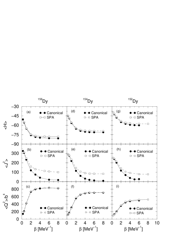
FIG. 1.: (a)-(c) Energy, spin, and quadrupole moment for ¹⁵⁶Dy. (d)-(f) Energy, spin, and quadrupole moment for ¹⁵⁴Dy. (g)-(i) Energy, spin, and quadrupole moment in ¹⁵²Dy.

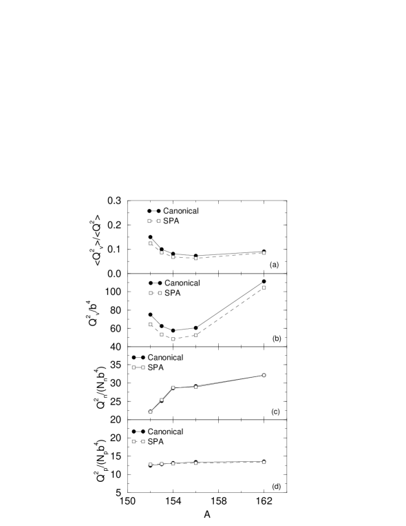
FIG. 2.: SPA and exact canonical solutions for quadrupole observables in selected dysprosium isotopes $A=152$ to $A=162$. All results are for $\beta=6$ or $T=0.167$ MeV. $\langle Q_{v}^{2}\rangle$ is defined as $(Q_{p}-Q_{v})^{2}$ and $b$ is the oscillator length.

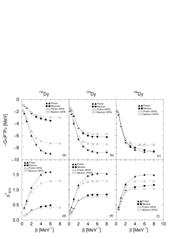
FIG. 3.: Pairing energy in ¹⁵²Dy (a), ¹⁵⁴Dy (b), and ¹⁵⁶Dy (c). BCS pair gaps are shown for ¹⁵²Dy (d), ¹⁵⁴Dy (e), and ¹⁵⁶Dy (f).

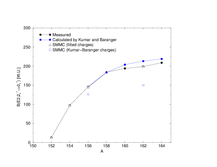
FIG. 4.: SMMC results for $B(E2;2_{1}^{+}\rightarrow 0_{1}^{+})$ for dysprosium isotopes. Results also shown in deformed cases (A=156, A=162) for strengths calculated with SMMC quadrupole moment and Kumar-Baranger effective charges.

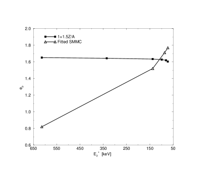
FIG. 5.: Effective charge vs. $E(2_{1}^{+})$ in Dy. Shown for Kumar-Baranger effective charge in deformed nuclei, $e_{p}=1+1.5Z/A$, and fitted SMMC charges. $E(2_{1}^{+})=614$ keV is spherical ¹⁵²Dy and $E(2_{1}^{+})=335$ keV is ¹⁵⁴Dy. The other points are for deformed ¹⁵⁶Dy and ¹⁶²Dy.

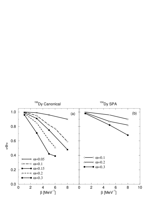
FIG. 6.: Monte Carlo sign for canonical (a) and SPA (b) cranking in ¹⁵⁶Dy.

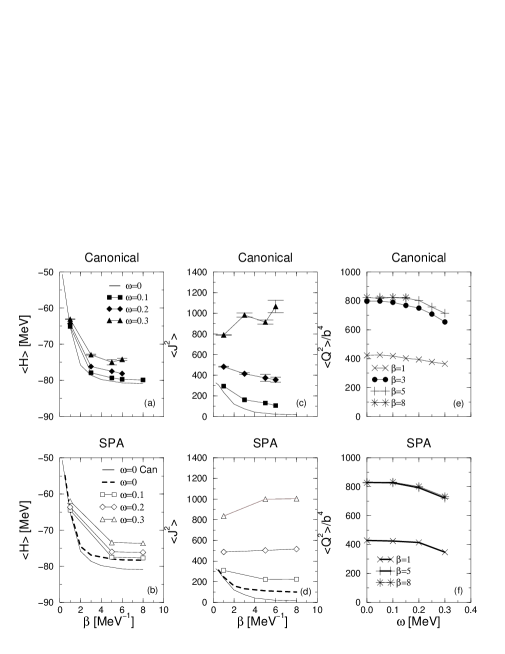
FIG. 7.: Canonical vs. SPA cranking results in ¹⁵⁶Dy for energy (a)-(b), spin (c)-(d), and quadrupole moment (e)-(f). Error bars are not shown for SPA results since error bars are smaller than the symbols.

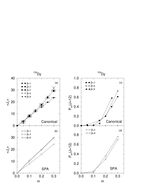
FIG. 8.: (a)-(b) $\langle J_{z}\rangle$ for canonical and SPA cranking in ¹⁵⁶Dy. (c)-(d) $J=12$ pair strength in canonical and SPA cranking in ¹⁵⁶Dy. $J=12$ pair strength comes exclusively from $i_{13/2}$.

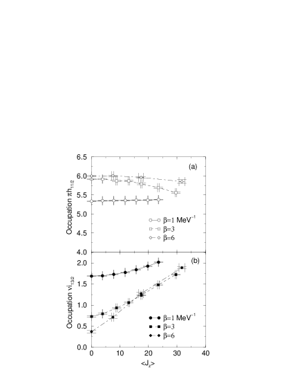
FIG. 9.: Occupation for proton $h_{11/2}$ (a) and neutron $i_{13/2}$ (b) vs. spin.

(a) ¹⁵²Dy, T$=0.25$ MeV            (b) ¹⁵²Dy, T$=0.5$ MeV                        

(c) ¹⁵²Dy, T$=2$ MeV            

FIG. 10.: (a) Shape at T=0.25 MeV for ¹⁵²Dy. Contour spacing is 0.79 MeV. (b) Shape at T=0.5 MeV for ¹⁵²Dy. Contour spacing is 0.64 MeV. (c) Shape at T=2 MeV for ¹⁵²Dy. Contour spacing is 2.9 MeV. Each plot is compiled from 2000 sample.

¹⁵⁴Dy at T$=0.133$ MeV

FIG. 11.: Shape at T=0.133 MeV for ¹⁵⁴Dy. 4800 samples. Contour spacing is 0.92 MeV.

¹⁵⁴Dy

(a) T$=0.25$ MeV, $\omega=0.05$ MeV^-1  (b) T$=0.25$ MeV, $\omega=0.1$ MeV^-1                                           (c) T$=0.25$ MeV, $\omega=0.2$ MeV^-1  (d) T$=0.5$ MeV, $\omega=0.05$ MeV^-1                                           (e) T$=0.5$ MeV, $\omega=0.2$ MeV^-1  (f) SPA: T$=0.125$ MeV, $\omega=0.6$ MeV^-1

FIG. 12.: (a) Shape at T=0.25 MeV and $\omega=0.05$ ($J\approx 6$) for ¹⁵⁴Dy. 2560 samples. Contour spacing is 2.9 MeV. (b) Shape at T=0.25 MeV and $\omega=0.1$ ($J\approx 8$) for ¹⁵⁴Dy. 2400 samples. Contour spacing 2.5 MeV. (c) Shape at T=0.25 MeV and $\omega=0.2$ for ¹⁵⁴Dy. 2400 samples. Contour spacing 2.4 MeV. (d) Shape at T=0.5 MeV and $\omega=0.05$ ($J\approx 10$) for ¹⁵⁴Dy. 3840 samples. Contour spacing 3.4 MeV. (e) Shape at T=0.5 MeV and $\omega=0.2$ ($J\approx 20$) for ¹⁵⁴Dy. 1920 samples. Contour spacing 4.2 MeV. (f) Shape at T=0.125 MeV and $\omega=0.6$ ($J\approx 50)$ for ¹⁵⁴Dy in SPA. Sign $\Phi=0.5$. 2000 samples. Contour spacing 1.2 MeV.

¹⁵⁶Dy

(a) T$=0.25$ MeV                                 (b) T$=0.5$ MeV                                          (c) T$=1$ MeV                                    (d) T$=0.125$ MeV, $\omega=0.1$ MeV^-1                        

FIG. 13.: Shape at T=0.25 MeV for ¹⁵⁶Dy. 2000 samples. Contour spacing is 6.5 MeV. Shape at T=0.5 MeV for ¹⁵⁶Dy. 2000 samples. Contour spacing is 6.9 MeV. Shape at T=1 MeV for ¹⁵⁶Dy. 2000 samples. Contour spacing is 2.0 MeV. Shape at T=0.125 MeV for ¹⁵⁶Dy with $\omega=0.1$ MeV^-1. 4800 samples. Contour spacing is 3.0 MeV.

¹⁴⁰Ba at T$=0.25$ MeV

FIG. 14.: Shape at T=0.25 MeV for ¹⁴⁰Ba. 4000 samples. Contour spacing 0.42 MeV.

¹⁴⁴Ba at T$=0.25$ MeV

FIG. 15.: Shape at $T=0.25$ MeV for ¹⁴⁴Ba. 2300 samples. Contour spacing is 0.7 MeV.

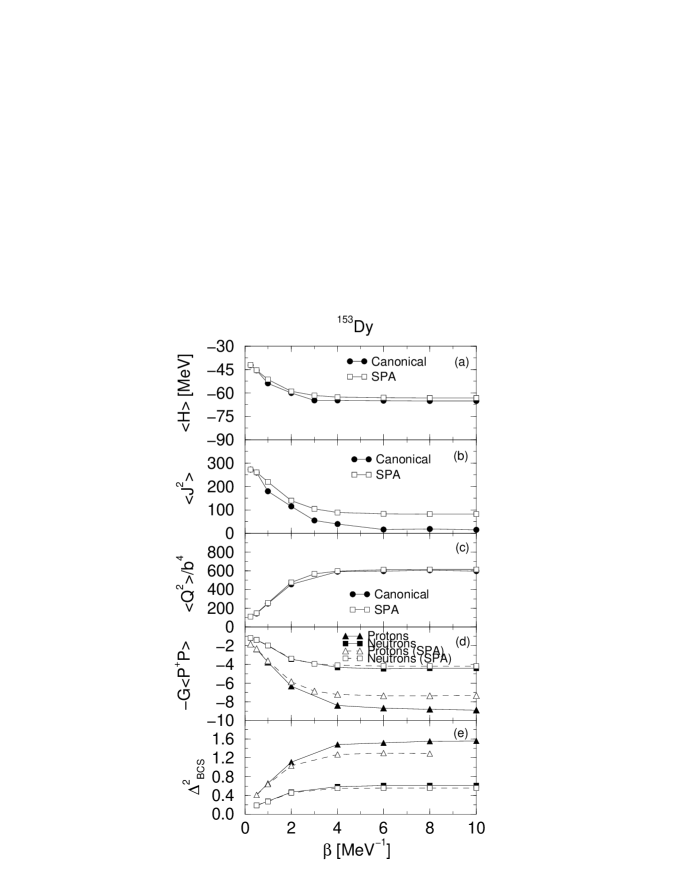
FIG. 16.: Energy (a), spin (b), quadrupole moment (c), pairing energy (d), and BCS pair gap (e) in ¹⁵³Dy for Kumar-Baranger interaction strengths. Symbols for $(e)$ match the symbols in $(d)$.

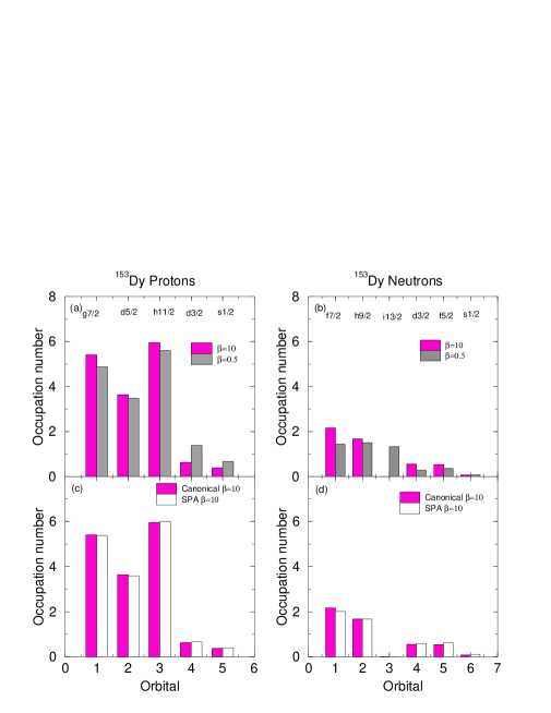
FIG. 17.: Proton and neutron occupations in ¹⁵³Dy. Results (a) and (b) are for the canonical ensemble at $T=0.1$ MeV and $T=2$ MeV while (c) and (d) are canonical vs. SPA at $T=0.1$ MeV.

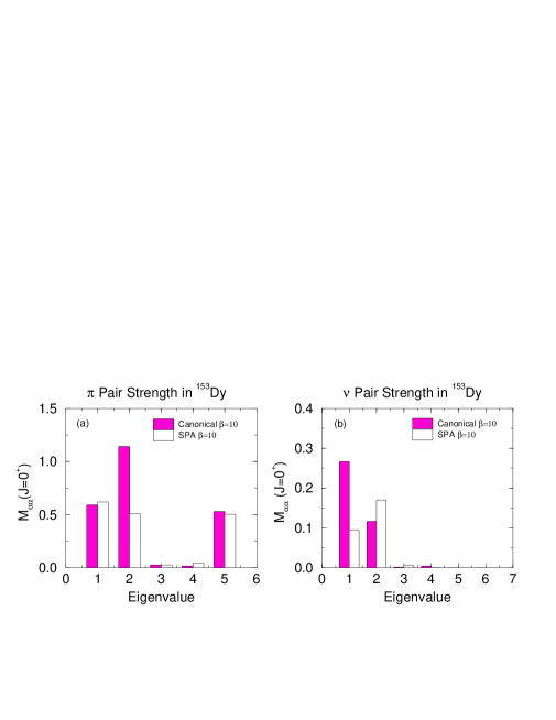
FIG. 18.: (a) Pairing matrix eigenvalues for protons in $J^{\pi}=0^{+}$ for ¹⁵³Dy at $T=.1$ MeV. (b) Pairing matrix eigenvalues for neutrons in $J^{\pi}=0^{+}$ for ¹⁵³Dy at $T=.1$ MeV.

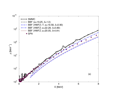
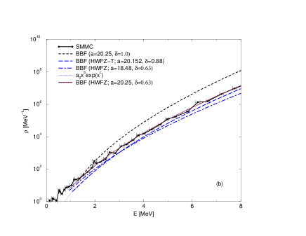
FIG. 19.: (a) Level density for ¹⁵⁴Dy in SMMC shown with backshifted Fermi gas approximations. BBF=standard backshifted Bethe formula. HFWZ=parameterization of Holmes, Woosley, Fowler, and Zimmerman, and HWFZ-T=HWFZ formula with Thielemann parameters. See text. HWFZ with $a=22.28$ is for spherical ¹⁵⁴Dy parameters while $a=20.05$ is for deformed ¹⁵⁴Dy parameters. SPA denotes the SPA result for the level density from SMMC. (b) SMMC result for ¹⁶²Dy compared with the same backshifted Bethe formula approximations.

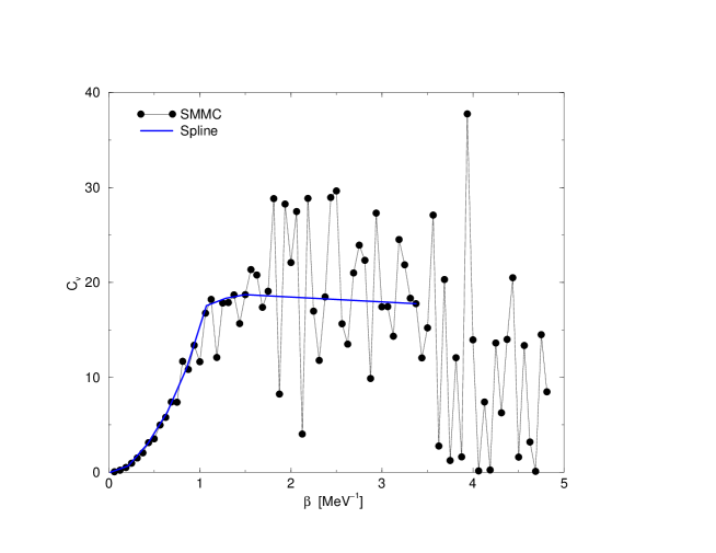
FIG. 20.: Heat capacity in ¹⁵⁴Dy.

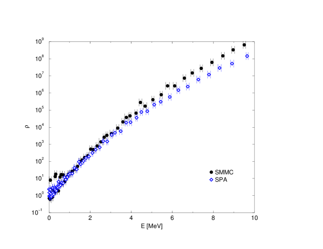
FIG. 21.: SPA heat capacity in ¹⁵⁴Dy.

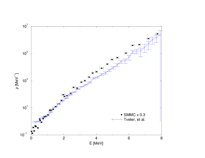
FIG. 22.: SMMC density vs. data in ¹⁶²Dy.

FIG. 23.: SMMC density in ¹⁴⁰Ba.

FIG. 24.: SMMC heat capacity in ¹⁴⁰Ba.

TABLE I.: SMMC $B(E2)$ vs. measured $B(E2;2_{1}^{+}\rightarrow 0_{1}^{+})$ with specified effective charges. $B(E2)$ in W.U. Errors are statistical Monte Carlo sampling errors. Column 6, $B(E2)$ for SMMC/KB $e_{p}(n)$, is the $B(E2)$ obtained from SMMC calculated quadrupole moments with Kumar-Baranger effective charges.

A	N	$e_{p}$	$e_{n}$	$B(E2)$	$B(E2)$	$B(E2)$
				SMMC	SMMC/KB $e_{p(n)}$	Expt
152	86	1	0	$13\pm 0.2$	N/A	13
154	88	1.5	0.5	$97\pm 0.2$	N/A	97
156	90	1.75	0.75	$146\pm 0.6$	$126.4\pm 0.5$	146
162	96	1.75	0.75	$199\pm 0.7$	$150.1\pm 0.5$	199

TABLE II.: Some spherical $E(2_{1}^{+})$ values from Kumar-Baranger [6]. Energies in keV.

	$E(2_{1}^{+})_{exp}$	$E(2_{1}^{+})_{th}$
138Ba	1438	2767
140Ba	602	2006
140Ce	1596	2531
142Ce	641	1772
144Ce	397	1095