Department of Physics and Astronomy 1998

ACCESSING THE SPACE–TIME DEVELOPMENT OF HEAVY–ION COLLISIONS WITH THEORY AND EXPERIMENT

David Alan Brown

Chapter 0 INTRODUCTION

1 Heavy-Ion Collisions

How does a colliding heavy-ion system evolve in space-time? This is an interesting question which we will discuss in this introduction. In the rest of this thesis, we will present work demonstrating how to access this space-time development using both theoretical and experimental techniques. This work falls into two categories: understanding transport-like models, with special emphasis on understanding their application to events at the Relativistic Heavy Ion Collider (RHIC) [BD98b], and understanding the use of Hanbury-Brown/Twiss (HBT) intensity interferometry as a way of working backwards from the data to the end of a heavy-ion collision [BD97, BD98a]. So, why should we be interested in heavy-ion collisions and why should we care how such a system evolves in space-time?

In a heavy-ion collision, the two colliding nuclei create an excited, dense and possibly thermalized, zone of nuclear matter in their wake. We see a much larger version of this in the effectively infinite thermalized nuclear matter of neutron stars, accretion disks and supernovas. We also expect that such matter existed moments after the Big Bang [Mül85, HM96]. In all of these cases, a reasonable description can be built up using single nucleon-nucleon collisions. Indeed, the systems created in heavy ion reactions are intermediate in size between single nucleon collisions and infinite thermalized nuclear matter and have features of both. Both single nucleon-nucleon collisions and heavy-ion collisions are easily accessible with current technology. Creating and manipulating infinite thermalized nuclear matter in a controlled way is far beyond anything possible today – we can not smash neutron stars together at will. In the absence of black hole/neutron star collider experiments, we must rely on extrapolation from finite nuclear systems.

Because the systems created in heavy-ion collisions are on the border of few particle systems and infinite thermalized nuclear matter, we expect that many of the features of both will show up in heavy-ion reactions. In particular, the thermal features of infinite matter should reveal themselves in some form in heavy-ion collisions. As an example, consider the liquid-gas phase-transition of nuclear matter – it is predicted to reveal itself through the processes of fragmentation and multifragmentation [Lyn98]. Another phase-transition, the Quark-Gluon Plasma (QGP) phase-transition is predicted to reveal itself by “fragmenting” into disordered Chiral Condensates or quark droplets [Raj95, HM96, McL86, Mül85]. The QGP phase transition is predicted by lattice QCD [DeT95, McL86, Mül85] and is implied by the hadronic model of Hagedorn [Hag65, Hag68, Hag71] and by Chiral Perturbation Theory [Raj95]. This phase transition is currently generating great interest as it may already be happening at CERN-SPS energies [RNC98] and should happen at both RHIC and the Large Hadron Collider (LHC) at CERN [HM96, McL86, Mül85]. A phase diagram of nuclear matter is shown in Figure 1. In this diagram, we see the two important phase transitions – the liquid gas phase transition and the transition to the QGP.

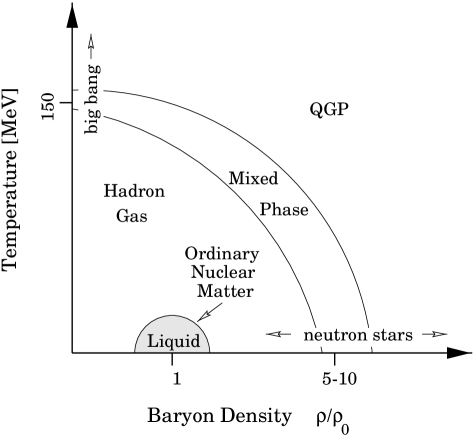
Figure 1: Phase diagram of nuclear matter. In this figure, $\rho$ is the baryon density and $\rho_{0}$ is normal nuclear matter density. The ground state of normal nuclear matter is the “liquid” phase.

Given that colliding heavy-ion systems are interesting, why study the space-time evolution of a heavy-ion collision? Well, the existence of a phase transition dramatically affects the space-time development of the system which in turn modifies the final state particle characteristics. Compare the two scenarios for a typical RHIC collision shown in Figure 2: on the left, the collision proceeds through a purely hadronic phase and, on the right, the system undergoes a phase-transition to the Quark-Gluon Plasma. Now, the existence of the phase-transition would lead to a drop in the pressure of the system at the phase-transition, softening the equation of state and leading to a disappearance of flow at the “softest point” [RPM⁺95, Ris96, RG96b, RG96a, R⁺96, Ris97]. Additionally, a phase-transition may lead to a long-lived system which would, in turn, lead to a larger relative emission point distribution for identical particle pairs [PCZ90]. This could be detected using HBT interferometry and nuclear imaging. The existence of a temporarily deconfined region would lead to other observable effects such as the color screening of the quarks in a $J/\psi$ particle. This then allows them to disassociate, leading to so-called $J/\psi$ suppression [MS86]. So, now it is clear that different physics leads to different space-time evolution of a collision. What we need now are ways to get at this space-time evolution.

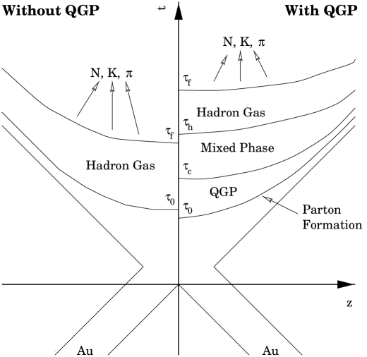
Figure 2: Space-time evolution of colliding heavy-ion system both with and without the QGP. In this figure, the important hypersurfaces are labeled with the proper time in the system CM. The time of full overlap of the two nuclei occurs at proper time $\tau_{0}$. The coexistence phase begins at proper time $\tau_{c}$ and hadronization begins at $\tau_{h}$. The collision ends at the freeze-out proper time $\tau_{f}$ when the final state nucleons and mesons stream out to the detector.

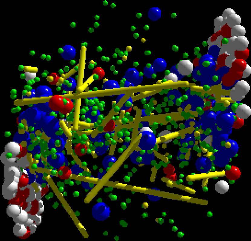
Figure 3: Sample UrQMD event: Au+Au at $E/A=200$ GeV and $b=5$ fm. In this picture, the small green spheres represent pions, the larger white and red spheres represent neutrons and protons, the larger blue spheres represent nucleon resonances and the yellow lines represent string excitations of the hadrons. In this picture, one can clearly see the spectator matter leaving the central collision zone. The large number of strings in the central region shows that there is a high energy density.

We can access the space-time evolution of a heavy-ion collision in several different ways. Two ways in particular are quite fruitful and are the subject of this thesis: 1) modeling the reaction using transport-like models and 2) accessing the final state directly using nuclear imaging. A large class of event generators are designed in order to study the phase-space densities of the particles as they evolve in time. Models that provide the time evolution of the phase-space particle densities are generally called transport models. In part, these models are useful because they provide a direct visualization of the collision (see for example the output from an UrQMD Au+Au event at $b=5$ fm and $E/A=200$ GeV in Figure 3 from [Web98]). More importantly however, such models can easily incorporate the data from single nucleon-nucleon collisions in vacuum, allowing us to build up a transport theory consistent with the underlying, elementary physics. A different and complementary approach is to directly image the reaction. By imaging the reaction, we directly get at the configuration space distribution of the system at freeze-out. Of course there are problems resulting from such an inversion of the experimental data resulting from the mixing of temporal evolution into the source in a nontrivial manner and the inherently difficulty of imaging resulting in rather crude images. Both the subjects of transport theory and nuclear imaging are discussed at length in this thesis.

2 Working Forwards – Theory

Modeling heavy-ion collisions has a long history, going back into the 1940’s. It has progressed to its current state by a series of improvements in our transport models and through theoretical insights into transport theory as a whole. However, the basic idea behind many of the models has remained more or less the same over the years: nucleons travel along their classical paths in configuration space and collide when particles are within $\sqrt{\sigma_{\mbox{\sc tot}}/\pi}$ of one another. The total collision cross section, $\sigma_{\rm TOT}$, is often tuned to reproduce single particle spectra. In other words, the nucleons are treated as an ensemble of “billiard balls” with radius $\sqrt{\sigma_{\rm TOT}/\pi}$ as they evolve in phase-space. This picture works well for nucleons at intermediate to high energies because they can be localized and interact on time scales much smaller than their mean free path. Should we expect this picture to work for the highest energy collisions? In these collisions, the criteria for closest approach breaks down [KBH⁺95] and the dynamics are dominated by massless (or nearly massless) particles which are both difficult to localize and may interact over large length and time scales. In other words, can the series of approximations used to arrive at this picture be justified for a RHIC collision where the majority of the interacting particles are quarks and gluons (i.e. partons)? Indeed, can we even define the initial conditions for a RHIC collision, a job tantamount to rewriting the parton model in phase-space?

The first models of heavy-ion collisions were based on the Internucleon Cascade (INC) concept developed by Serber in 1947 [Ser47]. His idea is simply to represent nucleons as “billiard balls” that travel along classical (relativistic) trajectories through configuration space. The nucleons interact strictly through binary collisions between nucleons at the point of closest approach in configuration space. This point of closest approach is defined through the total cross section to be $\sqrt{\sigma_{\rm TOT}/\pi}$; this model is the origin of the closest approach criteria. Collisions are the only way, in this model, to modify the momentum portion of the phase-space distribution. The INC concept has been extended into its modern-day incarnation by including resonances [CMV81, Cug82]. Because the particles do not interact through mean-fields, or any other higher order mechanisms, this model can only reproduce single particle observables such as spectra. Thus, it works best at energies where mean-field effects are small (i.e. $\gtrsim 1$ GeV). The concepts first laid out in this model form a blueprint for all the successful heavy-ion transport models to follow.

There are several models that build upon the basic ideas laid out in the INC and we will only discuss two classes of them: Quantum Molecular Dynamics and Boltzmann equation simulations. There are many other types of models, such as Time Dependent Hartree-Fock models, hydrodynamical models and thermal models, just to name a few. These models have varying degrees of success however none are as successful at reproducing single and many particle observables at intermediate to high energies ($\gtrsim 100$ MeV) as the classes of models that we discuss below.

Quantum Molecular Dynamics (QMD) models follow along much like the INC. In QMD, as in the INC, each nucleon is treated as a “billiard ball.” The particles are on-shell and all follow their classical equations of motion through configuration space. However, instead of using the cross sections to determine how a collision proceeds, QMD uses nucleon-nucleon potentials. QMD’s higher-energy incarnations, RQMD and UrQMD, supplement the nucleon-nucleon potentials with hard scattering through the cross sections using the closest approach criteria as in the INC [SBH⁺91, B⁺97] and with strings and resonances. RQMD and UrQMD also sport two other features, not present in INC: a nucleon mean field and Pauli blocking. With the inclusion of the mean field, both RQMD and UrQMD can reproduce flow observables, which are sensitive to mean field effects. The Pauli blocking only really helps at the lower energies, and the lack of Pauli blocking in the INC partially explains why the INC can not work well below 150–200 MeV/A. Both RQMD and UrQMD are significant advances over INC and are quite successful at reproducing single and multiple particle observables.

In Boltzmann-Uehling-Uhlenbeck (BUU) based approaches, such as in the MSU-BUU or the BEM models, one sets out to solve the BUU equation:

$$\begin{array}[]{rl}\displaystyle\frac{\partial f}{\partial t}+\vec{v}\cdot\vec{\nabla}_{r}f-\vec{\nabla}_{r}U\cdot\vec{\nabla}_{p}f=&\displaystyle-\frac{1}{(2\pi)^{6}}\int{d}^{3}p_{2}\>{d}^{3}p_{2^{\prime}}\>d\Omega\frac{d\sigma}{d\Omega}v_{12}\\ &\times\displaystyle\left\{\left[ff_{2}(1-f_{1^{\prime}})(1-f_{2^{\prime}})-f_{1^{\prime}}f_{2^{\prime}}(1-f_{1})(1-f_{2})\right]\right.\\ &\times\displaystyle\left.(2\pi)^{3}\delta^{3}\!\left(\vec{p}+\vec{p}_{2}-\vec{p}_{1^{\prime}}-\vec{p}_{2^{\prime}}\right)\right\}.\end{array}$$ (1)

In this equation, $f$ is the phase-space density. The particles are all taken to be on-shell and primes denote quantities to be taken after a collision between particles $1$ and $2$. This equation incorporates all of the important innovations included in the QMD and INC models, namely Pauli blocking, a mean field and the ability to fit results to known particle spectra. The factor $d\sigma/d\Omega$ is the experimentally determined nucleon-nucleon cross sections, although in practice, it may be altered to account for in-medium effects such as screening. The $(1-f)$ terms account for Pauli blocking in the final state; if a cell in phase-space is occupied by a Fermion, then in that region $f=1$ so $1-f=0$ making that collision term $0$. Finally we have the mean-field, $U$, which produces a driving force through the term $\vec{\nabla}_{r}U\cdot\vec{\nabla}_{p}f$. Now, the actual solving of the BUU equation varies with the model in question, but most models use the test-particle method. In this method, one replaces the phase-space distribution of particles with an ensemble of test-particles (essentially “billiard balls”). The test-particles follow classical trajectories that are modified by the mean-field driving force and interact using known cross sections in the same manner as the INC. Most BUU-type models are capable of reproducing both single particle spectra and flow observables.

Clearly, there are several features common to all of these models: classical relativistic kinetics, use of cross sections to constrain inter-particle interactions and full phase-space evolution of on-shell particle densities. How can we justify these features? For the INC and QMD based approaches, the justification is purely phenomenological. However, in BUU based approaches many features can be justified using known procedures and time-ordered non-equilibrium field theory [KB62, RS86, Dan84, BD72, KOH97, MD90, MH94]. So, we can study these works and understand how to justify the various features of transport models. In the standard derivations of the BUU equation the particles follow their classical trajectories only after applying the gradient approximation, an approximation also know as the Quasi-Classical Approximation (QCA). In this approximation, one throws away short scale structure in favor of large-scale structure in the densities and collision integrals. This washes out the quantum wanderings of particles from their classical paths. To justify this approximation, one needs the collision length scale to be much smaller than the length scale of variation of particle densities. Now the Lorentz dilation effects in an ultra-relativistic nuclear collision can ruin this scale separation by simultaneously shrinking the mean free path (the nucleon density increases by a factor of $\gamma$) and increasing the interaction time. A complementary approximation that one typically makes is the so-called Quasi-Particle Approximation (QPA). In this approximation, one replaces the full phase-space densities (i.e. in $E,\vec{p},t,$ and $\vec{x}$) with distributions of on-mass shell particles (so $E\equiv\sqrt{{\vec{p}}^{2}+m^{2}}$). This is equivalent to making all particles free particles with infinite lifetimes. Most theorists recognize this as a problem because even in intermediate energy collisions many off-shell and unstable particles exist (the resonances in particular). The persistence of off-shell and unstable particles means that subsequent interactions are not independent, making the interactions effectively many-body interactions. An example of this is the Landau-Pomeranchuk effect in a QED plasma. Suppose an electron is knocked off-mass-shell in a collision. In the vacuum, it would radiate a bremsstrahlung photon after some “formation-time.” In a dense plasma, it is possible for that electron to be struck again, before the “formation-time” has elapsed, both resetting “formation-time” clock and ensuring that that photon is not radiated. Thus, the subsequent electron interactions depend on the previous history of that electron. In both QMD and BUU type models, off shell evolution of unstable particles is included in some form by introducing a life-time parameter – when particles live too long, they are decayed. In the vacuum, particles are all on-shell and in momentum eigenstates so are spread over all configuration space. So, the QPA and QCA together act to scatter the particles as though they are in the vacuum, at least on the length scale of the interactions.

There is one feature that can not be justified on the basis of non-equilibrium field theory under any circumstances: the closest approach criteria. In practice, colliding particles when they are within the closest approach radius (i.e. $\sqrt{\sigma_{\rm TOT}/\pi}$) of one another is a purely phenomenological and conceptually simple way to implement the collision integrals in the BUU equations. At lower energies, use of this criteria causes no problems. However, at higher energies the closest approach radius acquires a frame dependence leading to the causality violations noted by Kortemeyer, et al. [KBH⁺95]. These violations grow more severe as the closest approach radius approaches the mean-free path of the particles in the simulation. Kortemeyer, et al. suggest several ways to avoid the causality violations but their solutions require a brute force suppression of the collisions that result in the violations rather than addressing the validity of the closest approach criteria. In the end, it is not clear whether the use of the closest approach criteria is a valid way to determine if two particles can collide.

Can these approximations be applied at RHIC energies to make a RHIC BUU model? Well, primary hadronic collisions in a typical nuclear reaction at RHIC will occur at $\sqrt{s}\sim 200A$ GeV. Such collisions are so violent that the partons, i.e. the quarks and gluons, comprising the hadrons will become deconfined. If the energy density is too low, the partons will immediately hadronize and the collision will presumably proceed as lower energy collisions do. However, if the energy density is high enough, the partons will remain deconfined and should form a quark-gluon plasma (QGP) [EW93, HM96, NR86]. In either case, we will need a transport model that can handle the partons. There have been several attempts to build a pure parton transport theory [Gei96, Hen95, HBFZ96, BI94], but each has their problems. Chief among these problems is that one either treats the soft long-range phenomena or one treats the hard short-distance phenomena, but never both in the same framework. Perhaps, by relaxing the need for a scale separation (and hence the QCA), we may be able to treat both hard and soft modes on equal footing. Additionally, we must relax the Quasi-Particle Approximation to allow for many-particle effects, such as the Landau-Pomeranchuk effect, which depend on particles being off-shell. Although the parton model is usually formulated with on-shell partons (i.e. in the Quasi-Particle Approximation), it has been known for some time that a proper covariant treatment of partons requires that the partons be allowed to be off-mass-shell [Lan77, SV93]. In fact, by allowing the partons to be off-shell, one can account for the apparent violation of the Gottfried sum rule and the relative depletion of Drell-Yan pairs at high $x_{F}$ in nuclear targets [SV93].

We do not have a phase-space treatment for QCD, but we have made several steps toward developing one for QED. In particular, we discuss how to create a transport theory for massless particles in Chapter 1 and we discuss issues related to constructing the parton model in phase-space in Chapter 2. The main result of both chapters is that the phase-space densities are convolutions of a phase-space source and a phase-space propagator. This “source-propagator” picture should lead to an improved transport theory for the massless partons at RHIC as it can handle both soft and hard modes simultaneously. The “source-propagator” picture is covariant, so does not suffer from the causality violations of standard transport approaches. So, in the end we may not have all the answers for what a transport model at RHIC would be, but we have made several steps in the right direction.

3 Working Backward – Experiment

Being able to watch a system evolve on the computer definitely helps to visualize the events during a collision, but it pales in comparison to directly imaging the reaction. The technique of intensity interferometry allows us to take a large step toward this goal. Astronomers have long recognized the value of intensity interferometry. In fact, it was a pair of astronomers who developed the technique: Robert Hanbury-Brown and Richard Twiss [HBJDG52, HBT54, HBT56b, HBT56a, HBT56c, HBT57a, HBT57b]. The application of intensity interferometry to nuclear collisions followed a few years after Hanbury-Brown and Twiss’s initial discovery [G⁺59, GGLP60]. Until recently the goal of nuclear interferometry did not differ greatly from Hanbury-Brown and Twiss’s original goal; they measured the radius of Sirius while we typically measure the radius of the relative emission profile of particle pairs (the source function) in heavy-ion reactions. We have recently demonstrated how to move beyond simply extracting source radii to extracting the entire source function from the experimental data [BD97, BD98a].

Intensity interferometry is based on a fairly simple observation. If we have two possible events, say detection of one pion in detector 1 and detection of a second pion in detector 2, the probabilities of each occurring are uncorrelated if the probability of both happening is the product of the probability of each happening individually:

$$P_{12}=P_{1}P_{2}.$$

On the other hand, if they are correlated then this is not true. In this case, we can define the correlation function as the ratio

$$C_{12}=\frac{P_{12}}{P_{1}P_{2}}.$$

Then $C_{12}=1$ if the two events are totally uncorrelated.

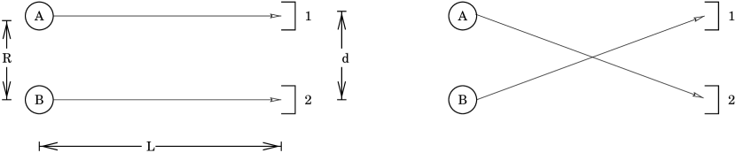
Figure 4: A simple example illustrating the HBT effect.

It is useful to illustrate this point with an example. This example is given in [Bay98] and pictured in Figure 4. In this figure, we have two sources of photons labeled A and B and two photon detectors labeled 1 and 2. Now, suppose A and B emit the photons in spherical waves and bunched in time. The amplitude for receiving a photon from A in detector 1 is

$$C_{A}\frac{\exp[{ir_{A1}k+i\phi_{A}}]}{r_{A1}}$$

so the total amplitude at detector 1 is (assuming $L\gg d,R$)

$$A_{1}=\frac{1}{L}\left(C_{A}\exp[ir_{A1}k+i\phi_{A}]+C_{B}\exp[ir_{B1}k+i\phi_{B}]\right)$$

and similarly for detector 2. Here, the phase $\phi$ is random and changes with each bunch. So, detector 1 receives photon hits with a probability (or intensity) of

$$\begin{split}I_{1}=|A_{1}|^{2}=&\frac{1}{L^{2}}\left(|C_{A}|^{2}+|C_{B}|^{2}+C_{A}^{*}C_{B}\exp[i((r_{B1}-r_{A1})k+\phi_{B}-\phi_{A})]\right.\\ &+\left.C_{A}C_{B}^{*}\exp[-i((r_{B1}-r_{A1})k+\phi_{B}-\phi_{A})]\right)\end{split}$$

and similarly for detector 2. Now averaging over many sets of bunches, each with different phases, we find the average intensity in any one detector to be

$$\left<I_{1}\right>=\left<I_{2}\right>=\frac{1}{L^{2}}\left(\left<|C_{A}|^{2}\right>+\left<|C_{B}|^{2}\right>\right).$$

Now, if instead of averaging the intensities, we were to average the quantity $I_{1}I_{2}$, we would find that $\left<I_{1}I_{2}\right>\neq\left<I_{1}\right>\left<I_{2}\right>$ as we would expect for uncorrelated sources. In fact, we would find

$$\frac{\left<I_{1}I_{2}\right>}{\left<I_{1}\right>\left<I_{2}\right>}=1+2\frac{\left<|C_{A}|^{2}\right>\left<|C_{B}|^{2}\right>}{\left(\left<|C_{A}|^{2}\right>+\left<|C_{B}|^{2}\right>\right)^{2}}\cos[k(r_{A1}-r_{A2}-r_{B1}+r_{B2})].$$

This second term is the interesting one as it is purely quantum in origin and because it is sensitive to the separation of the two sources. In practice, the ratio $\left<I_{1}I_{2}\right>/\left<I_{1}\right>\left<I_{2}\right>$ is defined as the correlation function $C_{12}$.

This example illustrates a simplified form of what Hanbury-Brown and Twiss observed in their series of pioneering experiments into intensity interferometry [HBJDG52, HBT54, HBT56b, HBT56a, HBT56c, HBT57a, HBT57b]. The culmination of their experiments was the determination of the angular diameter of the star Sirius using a pair of World War II surplus searchlight mirrors and some electronics [HBT56b]. The radius they found to be $0.0068^{\prime\prime}\pm 0.0005^{\prime\prime}$ or $3.1\times 10^{-8}$ radians. At a distance of $2.7$ pc $=8.5$ lyrs, Sirius is a mere $3.7$ times the radius of our sun. As a result of their work, the technique of intensity interferometry became known as the HBT effect.

The HBT effect was first noted in subatomic physics in a study of the Bose-Einstein symmetrization effects on pion emission in proton-antiproton annihilation [G⁺59]. To explain the data Goldhaber, Goldhaber, Lee and Pais [GGLP60] used a static source model for pion emission and determined the effect on the angular distribution of pions due to symmetrization. For a time, the effect was known as the GGLP effect. While Kopylev and Podgoretski first described how interferometry is sensitive to the size of the emission region of a heavy-ion collision [KP71, GKP71, Kop72, KP72, KP73, Kop74], the GGLP effect first was explained in terms of intensity interferometry by Shuryak [Shu73a, Shu73b] and Cocconi [Coc74]. In the late 70’s and early 80’s the ranks of particles where the HBT effect was observed grew to include protons, intermediate mass fragments (IMF’s) and neutrons. Today interferometry is carried out with a wide array of particles, including (but not limited to) kaons, leptons, photons, and even pairs of unlike particles.

While the experimental community advanced dramatically in its ability to measure correlation functions, the amount of information gleaned from an individual correlation function has not advanced much at all; until recently, people still used the correlation function only to get the radius (or mean life-time) and $r=0$ intercepts of the source function. This is of course the obvious thing to do because most correlation functions (at least for pions) look like Gaussians after a Coulomb correction. One can get a lot of information from a radius, especially when the data is cut on the right kinematic variables. Nevertheless, in many cases, one is replacing 50 points of a well defined function with one radius – a great waste of information. There are of course exceptions to this rule: Pratt [PCZ90] developed a series of codes to convert output from transport models to correlation functions which can then be directly compared to data. Beyond this, it is only lately that people have tried to go beyond simply fitting a radius: Nickerson, Csörgő and Kiang have attempted fitting correlation functions to a Gaussian plus an exponential halo [NCK98] and Wiedermann and Heinz have proposed performing a moment expansion of the correlation functions [WH96]. While both of these are valuable exercises, neither make full use of the data. This is why my advisor, Paweł Danielewicz, and I proposed doing nuclear imaging.

Nuclear imaging amounts to reconstructing the relative emission distribution for the pairs used to construct the correlation function. Imaging relies on the observation that the source function and the correlation function are related through a simple integral equation which can be inverted. We discuss the methods for doing this inversion and the results we get from the inversion in Chapter 3.

4 Overview of Thesis

This thesis is about the tools we use to investigate the space-time developments of heavy-ion reactions. Specifically, we discuss the application of transport theory to parton dominated collisions at RHIC and the LHC and we discuss the application of imaging techniques to HBT intensity interferometry. Both lines of research are aimed at deducing the features of the phase-space particle densities and how they evolve as a heavy-ion collision proceeds.

In the second chapter, we describe some of the things needed to derive a QCD transport theory. We begin by defining the phase-space particle densities as understanding their time-evolution is the ultimate goal when building transport models. We then describe the contour Green’s functions and the other Green’s functions that we need to perform actual calculations of the densities. We will then spend the rest of the chapter deriving a QED transport theory valid for massless photons and electrons but without applying either the Quasi-Particle or the Quasi-Classical (or gradient) approximations. In doing so, we derive the Generalized Fluctuation-Dissipation theorem – proving that a phase-space density is the convolution of a phase-space source density with a phase-space propagator. This is a general result, applicable to QCD as well as to particles with mass. We use this theorem to create QED phase space evolution equations and to illustrate the perturbative solution for the photon and electron densities that we discuss in Chapter 2. Finally, we describe how one might make a transport model based on these results.

We will need phase-space parton densities for input in a parton transport model so in the third chapter we begin the process of recasting the parton model in phase-space. The parton model has two key components: factorization of the cross sections and evolution of the parton densities. The first component has a QED analogy in the Weizsäcker-Williams approximation: in the Weizsäcker-Williams approximation, the cross section for a photon mediated process is the convolution of a photon density and the cross section for the photon induced sub-process. We rederive the Weizsäcker-Williams approximation in phase-space, applying it to both the photon cloud and electron clouds of a point charge. In the process, we not only illustrate how to rewrite things in phase-space, but we investigate the roles of phase-space sources and propagators. The second component, evolution of the parton densities, can also be investigated in QED. The renormalization group evolution of the parton densities is equivalent to the summation of a class of ladder diagrams in the Leading Logarithm Approximation. We can study a simplified version of the ladder diagrams in QED by calculating the photon and electron phase-space densities around a point charge. Indeed, the electron and photons surrounding a point charge are point-like “constituents” of the point charge, so they earn the right to be called QED partons. Finally, with all of this QED experience, we discuss the main features of the phase-space parton distribution of a nucleon in the Leading Logarithm Approximation.

In the fourth chapter, we describe how nuclear imaging can be used to extract the source function from correlation data. We list the methods we have used to perform this inversion, describing what works and how and why they work. In particular, we will discuss the role of constraints in the stabilization of the inversion and the method Paweł Danielewicz developed which works well even without constraints. Next, we discuss what other quantities can be extracted from the images. Finally, we apply our inversion techniques to various data sets and discuss what the images mean.

We will conclude the thesis with a brief summary and a description of what work needs to be done to follow up the lines of investigation opened here.

There are also several appendices exploring various side and technical issues. Among these are discussion and derivations of the phase-space propagators, the measurables in a heavy-ion collision, the cross section in terms of phase-space densities, the Coulomb field of a static point charge in phase-space, the gauge dependence of the photon distributions from Chapter 2 and both wavepackets in phase-space and current densities in phase-space.

Throughout this thesis, we use natural units ($\hbar=c=1$) when convenient, but we insert factors of $\hbar c$ when we need an energy or length in conventional units. The signature of the metric tensor is $(+,-,-,-)$.

Chapter 1 EVOLUTION OF PHASE-SPACE PARTICLE DENSITIES

How can we go beyond standard transport methods to produce a transport-like theory for massless (or nearly massless) particles in ultra-relativistic heavy-ion collisions? However we do it, this theory must allow for off-shell evolution of the particle densities so we must relax the Quasi-Particle Approximation. This theory must also deal with all hard and soft modes on equal footing. Since the modes act on different length and time scales, the theory must not require scale separation or use the Quasi-Classical Approximation. The way we produce our transport-like theory is to go back to the original work on transport, identify where the QCA and QPA approximations are made, and replace them with more suitable approximations. We use QED for this study because it is not as complicated as QCD but still contains many of the relevant features of QCD. By not making the standard approximations in our study of QED transport, we will find that the densities take a “source-propagator” form – meaning a phase-space density is the convolution of a phase-space source density and a phase-space propagator. As the reader will see, the phase-space source gives the quasi-probability density for creating a particle with a particular momentum. The propagator then sends this particle from its creation point across a space-time displacement to the observation point. This “source-propagator” form is a general result, not specific to QED, and it is encoded in the key result of this chapter: the phase-space Generalized Fluctuation-Dissipation Theorem.

To begin, we define the initial state through the density matrix and the particle phase-space densities as expectation values with the density matrix. Because of the general nature of the density matrix we can simultaneously investigate anything from single states to ensembles of states. The densities themselves are Wigner transforms of two-point functions such as $G^{\gtrless}(x_{1},x_{2})$. We will discuss these densities, how they relate to other possible definitions of the particle densities, and how one normally implements the Quasi-Particle Approximation.

To perform practical calculations of the $G^{\gtrless}$, we introduce the contour Green’s functions. These Green’s functions are defined on a contour in the complex time plane. By restricting the arguments of the contour Green’s function to various branches of the contour, we can define other auxiliary Green’s functions such as Feynman’s Green’s functions. At this point, we also introduce the retarded Green’s functions as they will play a dominant role in later discussions. The introduction of the complex time contour also leads to a simple scheme for perturbatively calculating the contour Green’s functions. This in turn leads to the Dyson-Schwinger equations which are the starting point for the derivation of the semi-classical transport equations.

After these preliminaries, we begin examining QED transport theory for massless particles. In Section 1, we follow essentially the standard semi-classical transport equation derivation: we derive the Kadanoff-Baym equations and formally solve them to get the Generalized Fluctuation-Dissipation Theorem. Unlike conventional derivations of transport theory, at this point we do not make the Quasi-Classical Approximation. This approximation amounts to ignoring small-scale structure of the particle phase-space densities, resulting in much simpler collision integrals [Dan84, MH94]. By not making this approximation, we arrive at the Generalized Fluctuation-Dissipation Theorem which codifies the “source-propagator” picture of the particle densities. Crucial inputs to the theorem are the phase-space sources; we will discuss how to calculate them.

With the sources and the Generalized Fluctuation-Dissipation Theorem, we derive a set of phase-space QED evolution equations. These evolution equations describe the evolution of the system in phase-space from the distant past to the present, including all splittings, recombinations and scatterings. Furthermore, we can expand these evolution equations to get the lowest order contributions to the particle densities or we can differentiate the evolution equations to get transport equations. All of these results are manifestly Lorentz covariant so do not suffer from the causality violation of a more traditional approach. However, our investigation is not as mature as conventional transport approaches and we are not at the stage where we can make quantitative predictions.

For those familiar with the common steps in deriving semi-classical transport equations from the Kadanoff-Baym equations, we suggest skipping past Section 4 to Section 5.

1 The Density Matrix

The systems that we study range from the very simple, i.e. binary collisions, to the very complex, i.e. interacting heavy-ion systems. We could deal with the potential complexity right up front by specifying the incoming states, or we could cleverly lump the complexity into a density matrix. We choose the latter because it is both more general and simpler to do.

First we write the density matrix $\hat{\rho}$ as

$$\hat{\rho}=\sum_{{\rm all\;states}}\left|m\right>\left<n\right|\rho_{mn}.$$ (1)

Here, the states $\left|m\right>$ and $\left|n\right>$ can correspond to single particle or many particle states, depending on the system of interest.

Because the density matrix is so general, we can treat many different situations at the same time, all within one general framework. For example, we can easily incorporate a thermal population of states for work with infinite thermalized nuclear matter. As a second example, we can account for correlated initial and final states as well as bound states using an appropriate choice of density matrix. As a final example, we can choose suitable density matrices to give us localized wavepackets of single particles in the initial state. It is this last reason that we will take advantage of in this thesis. In every subsequent chapter, the particles we consider will be localized in space and or momentum (or both!). In fact, we demonstrate how to make a wavepacket localized in phase-space in Appendix 11. In this chapter and the following chapter we create particle phase-space densities that are localized both in momentum and coordinates and in Chapter 3 we will measure the localized sources of particles created in heavy-ion reactions.

For now, we leave the density matrix in this general form. The only condition that we place on it is that we can perform a Wick decomposition on general expectation values. This requirement is important for creating a perturbation expansion of the expectation values [Dan84]. The discussion of what density matrices allow a Wick decomposition is carried out elsewhere [Dan84, CSHY85, Sch94].

Now, in terms of this density matrix, we can define an arbitrary expectation value of an Heisenberg picture operator:

$$\left<\hat{\cal O}_{H}\right>=\frac{{\rm Tr}\left(\hat{\rho}\hat{\cal O}_{H}\right)}{{\rm Tr}(\hat{\rho})}.$$ (2)

As a simple example of both a density matrix and an expectation value, consider the density matrix containing only the vacuum state, $\left|0\right>$: $\hat{\rho}=\left|0\right>\left<0\right|$. The trace over this density matrix gives the vacuum expectation value of the operator

$$\left<\hat{\cal O}_{H}\right>=\frac{{\rm Tr}\left(\hat{\rho}\hat{\cal O}_{H}\right)}{{\rm Tr}(\hat{\rho})}=\frac{\left<0\right|\hat{\cal O}_{H}\left|0\right>}{\left<\left.0\right|0\right>}.$$

2 Particle Phase-Space Densities

Since our ultimate goal is to follow the phase-space densities, we would like to define them precisely. We will define them as the Wigner transforms of certain two-point functions. These two-point functions, also known as the $>$ and $<$ Green’s functions are for scalar bosons:

$$i{G}^{>}\!\left(x,y\right)= \left<\hat{\phi}(x)\hat{\phi}^{*}(y)\right>$$ (3a)

$$i{G}^{<}\!\left(x,y\right)= \left<\hat{\phi}^{*}(y)\hat{\phi}(x)\right>,$$ (3b)

for vector bosons (such as photons):

$$i{D}^{>}_{\mu\nu}\!\left(x,y\right)= \left<\hat{A}_{\mu}(x)\hat{A}_{\nu}(y)\right>-\left<\hat{A}_{\mu}(x)\right>\left<\hat{A}_{\nu}(y)\right>$$ (3c)

$$i{D}^{<}_{\mu\nu}\!\left(x,y\right)= \left<\hat{A}_{\nu}(y)\hat{A}_{\mu}(x)\right>-\left<\hat{A}_{\mu}(x)\right>\left<\hat{A}_{\nu}(y)\right>,$$ (3d)

and for fermions (such as electrons or nucleons):

$$i{S}^{>}_{\alpha\beta}\!\left(x,y\right)= \left<\hat{\psi}_{\alpha}(x)\hat{\bar{\psi}}_{\beta}(y)\right>$$ (3e)

$$i{S}^{<}_{\alpha\beta}\!\left(x,y\right)= -\left<\hat{\bar{\psi}}_{\beta}(y)\hat{\psi}_{\alpha}(x)\right>.$$ (3f)

The field operators in these expressions are taken in the Heisenberg picture. Note that, because of the equal time commutation relations for the interaction picture operators, if we write the above in the interaction picture, we find ${G}^{>}\!\left(x,y\right)={G}^{<}\!\left(y,x\right)$ for both fermions and bosons.

These Green’s functions are hermitian and they contain the complete single-particle information of the system. For example, setting $x=y$ gives us the single particle density matrix. Furthermore, Wigner transforming in the relative coordinate, we find the off-mass shell generalization of the Wigner function for the particles – in other words, the phase-space density. Let us demonstrate for scalar fields:

$$\begin{split}f(x,p)&=i{G}^{<}\!\left(x,p\right)\\ &=\int{d}^{4}(x-y)\>e^{i(x-y)\cdot p}i{G}^{<}\!\left(x,y\right)\\ &=\int{d}^{4}(x-y)\>e^{i(x-y)\cdot p}\left<\hat{\phi}^{*}(y)\hat{\phi}(x)\right>.\end{split}$$ (4)

We identify $f(x,p)$ with the number density of particle (or antiparticles) per unit volume in phase-space per unit invariant mass squared at time $x_{0}$:

$$f(x,p)=\frac{dn(x,p)}{d^{3}x\>d^{3}p\>dp^{2}}$$

In particular, for $p_{0}>0$, $i{G}^{<}\!\left(x,p\right)$ is associated with the particle densities and $i{G}^{>}\!\left(x,p\right)$ is associated with the hole density. For $p_{0}<0$, $i{G}^{<}\!\left(x,p\right)$ is the anti-hole density and $i{G}^{>}\!\left(x,p\right)$ is the anti-particle density. The photon and electron densities are defined in the same way, however because of their more complicated spin structure, their Wigner functions carry indices.

Other, gauge invariant, definitions of the particle densities exist in the literature [ZH96, VGE87, EGV86a, EGV86b]. However, while these distributions are gauge invariant, they do not obey simple Dyson-Schwinger equations and so it is difficult to derive transport theory from them. Since all of the observables in which we are interested are gauge invariant and all of the equations involving the densities that we derive are gauge covariant, we do not need to resort to exotic definitions of the densities.

The off-shell Wigner function is related to the conventional Wigner function, $f_{0}(x,\vec{p})$, through the invariant mass integration:

$$f_{0}(x,\vec{p})=\frac{dn(x_{0},\vec{x},\vec{p})}{d^{3}x\>d^{3}p}=\int^{\infty}_{-\infty}dp^{2}f(x,p).$$ (5)

In the Quasi-Particle Approximation we assume that

$$f(x,p)\approx\begin{cases}f_{0}(x,\vec{p})\delta(p^{2}-m^{2}_{*})&\text{for $p_{0}>0$}\\ -(1-f_{0}(x,\vec{p}))\delta(p^{2}-m^{2}_{*})&\text{for $p_{0}<0$.}\end{cases}$$ (6)

In this approximation (which is quite a common approximation in transport-like models), $f(x,p)$ and $f_{0}(x,\vec{p})$ are interchangeable. Here $m_{*}$ is the effective mass of the particle and it may be either the mass in free space or it may contain in-medium modifications.

Now, finding the particle densities are the ultimate goal of our work. We will describe several ways to calculate them in the following chapters. To this end, we will need several of the Green’s functions in the next subsection. Also, given that we measure the densities in any experiment, we discuss particle spectra (basically the momentum space density of particles) in great detail in the Appendix 6.

3 Other Green’s Functions

In order to calculate the densities, we will need to introduce several other Green’s functions. The first of these, the contour Green’s functions, are the most exotic as they are defined on a contour on the complex time plane. To see why such a contour is useful, we will first discuss the expectation value of an arbitrary Heisenberg operator $\hat{\cal O}_{H}(t)$. With an understanding of why this contour is used, we will define the contour Green’s functions and all of the auxiliary Green’s functions that the contour Green’s functions encapsulate.

1 Operator Expectation Values

Consider the expectation value of an Heisenberg picture operator with one time argument:

$$\left<\hat{\cal O}_{H}(t)\right>=\frac{{\rm Tr}\left(\hat{\rho}\hat{\cal O}_{H}(t)\right)}{{\rm Tr}(\hat{\rho})}.$$ (7)

This operator could be anything from the energy density of the system to the number operator of a specific field provided that is a function of one time variable only.

The simplest way to evaluate this operator is to rewrite the operator in the interaction representation. Once in the interaction picture, we can perform a perturbative expansion of the time evolution operator and develop successive approximations to the expectation value. The relation between an operator in the Heisenberg and interaction pictures is

$$\hat{\cal O}_{H}(t)=\hat{U}(t_{0},t)\hat{\cal O}_{I}(t)\hat{U}(t,t_{0})$$ (8)

where $\hat{U}(t,t_{0})$ is the interaction picture time evolution operator and $t_{0}$ is the time at which the two pictures coincide. For $t>t_{0}$, the evolution operator is given in terms of the interaction part of the Hamiltonian in the interaction representation by

$$\hat{U}(t,t_{0})={\rm T}^{c}\left[\exp\left(-i\int^{t}_{t_{0}}dt^{\prime}\hat{H}_{I}^{I}(t^{\prime})\right)\right].$$ (9)

The operator ${\rm T}^{c(a)}$ simply orders the operators in the expectation value in a chronological (or anti-chronological) fashion. In other words:

$${\rm T}^{c}\left(\hat{A}(t_{1})\hat{B}(t_{2})\right) =\theta(t_{1}-t_{2})\hat{A}(t_{1})\hat{B}(t_{2})+\theta(t_{2}-t_{1})\hat{B}(t_{2})\hat{A}(t_{1})$$ (10a)

$${\rm T}^{a}\left(\hat{A}(t_{1})\hat{B}(t_{2})\right) =\theta(t_{1}-t_{2})\hat{B}(t_{2})\hat{A}(t_{1})+\theta(t_{2}-t_{1})\hat{A}(t_{1})\hat{B}(t_{2})$$ (10b)

So, we can write the expectation value of $\hat{\cal O}_{H}(t)$ in the interaction picture as follows:

$$\begin{array}[]{rl}\displaystyle\left<\hat{\cal O}_{H}(t)\right>&=\displaystyle\left<\hat{U}(t_{0},t)\hat{\cal O}_{I}(t)\hat{U}(t,t_{0})\right>\\ &=\displaystyle\left<{\rm T}^{a}\left[\exp\left(-i\int^{t_{0}}_{t}dt^{\prime}\hat{H}_{I}^{I}(t^{\prime})\right)\right]\hat{\cal O}_{I}(t){\rm T}^{c}\left[\exp\left(-i\int^{t}_{t_{0}}dt^{\prime}\hat{H}_{I}^{I}(t^{\prime})\right)\right]\right>\end{array}$$ (11)

Notice that the time ordering goes as follows from right to left: the rightmost time evolution operator takes things from $t_{0}$ forward in time to $t$ where the operator is evaluated then the second time evolution operator takes things from $t$, backwards in time again to $t_{0}$. We can simplify notation by introducing a contour in the complex time plane which runs from $t_{0}$ up to $t$ and back again to $t_{0}$ as shown in Figure 1.

Figure 1: Contour in the complex time plane for evaluating operator expectation values. The upper branch corresponds to causal ordering and the lower branch to anti-causal ordering. The arrows denote the contour ordering enforced by the $\rm T$ operator.

We can define ordering along this contour using the contour time-ordering operator, T, defined via

$${\rm T}\left(\hat{A}(t_{1})\hat{B}(t_{2})\right)=\theta(t_{1},t_{2})\hat{A}(t_{1})\hat{B}(t_{2})+\theta(t_{2},t_{1})\hat{B}(t_{2})\hat{A}(t_{1})$$ (12)

where the contour theta function is given by

$$\theta(x_{0},y_{0})=\left\{\begin{array}[]{ll}1&\mbox{if $x_{0}$ is later on the contour than $y_{0}$}\\ 0&\mbox{otherwise}\end{array}\right.$$

Using this notation, Equation (11) simplifies to

$$\left<\hat{\cal O}_{H}(t)\right>=\left<{\rm T}\left[\exp\left(-i\int_{\cal C}dt^{\prime}\hat{H}_{I}^{I}(t^{\prime})\right)\hat{\cal O}_{I}(t)\right]\right>$$ (13)

This idea of a contour that zig zags back and forth along the real time axis, encapsulating the various time orderings needed in an expectation value was first noticed by Schwinger [Sch61]. The idea was generalized by Danielewicz [Dan90] to account for operators with multiple time arguments.

Now we will not actually demonstrate how to solve for $\left<\hat{\cal O}_{H}(t)\right>$, although it is discussed in several places, notably [Sch61] and [FW71]. However, our discussion is a useful motivation for the introduction of the contour ordering that we use to define the contour Green’s functions in the next section.

2 Contour Green’s Functions

Introducing the time ordering along a contour in the complex time plane is a clever way to express expectation values and what makes the ordering so clever is the way the two branches encode causal or anti-causal time orderings. Let us take advantage of this feature and define the contour Green’s functions as Green’s functions that are ordered along the time contour:

$$i{G}\!\left(x,y\right)=\left<T\hat{\phi}(x)\hat{\phi}^{*}(y)\right>$$ (14a)

for scalar particles,

$$i{D}_{\mu\nu}\!\left(x,y\right)=\left<T\hat{A}_{\mu}(x)\hat{A}_{\nu}(y)\right>-\left<\hat{A}_{\mu}(x)\right>\left<\hat{A}_{\nu}(x)\right>$$ (14b)

for photons and

$$i{S}_{\alpha\beta}\!\left(x,y\right)=\left<T\hat{\psi}_{\alpha}(x)\hat{\bar{\psi}}_{\beta}(y)\right>$$ (14c)

for fermions. For practical purposes, we must take the lower limit of the contour as $t_{0}\rightarrow-\infty$, where we specify the initial conditions in the density matrix. Furthermore, we must take the upper limit of the contour as $t\rightarrow\infty$ to ensure that all of the time arguments of the contour Green’s functions are between the limits $t_{0}$ and $t$ and thus are on the contour.

All of the above Green’s functions can be written in the interaction picture in a manner analogous to Equation (13). From this, Danielewicz [Dan84] has derived the set of Feynman rules for evaluating the contour Green’s functions. These rules differ slightly from the Feynman rules for the S-matrices found in most field theory books, so we tabulate the QED rules in the next section.

The contour Green’s function can be written in terms of the $\gtrless$ Green’s functions as

$${G}\!\left(x,y\right)=\theta(x_{0},y_{0}){G}^{>}\!\left(x,y\right)+\theta(y_{0},x_{0}){G}^{<}\!\left(x,y\right)$$ (15)

for both fermions and bosons. By virtue of this, we have the relation ${G}\!\left(x,y\right)={G}\!\left(y,x\right)$.

3 Contour Feynman Rules for Quantum Electrodynamics

In order to evaluate the contour Green’s functions in the interaction picture, we need a set of Feynman rules for these Green’s functions. These rules have been derived previously [Dan84] so we may just state them here. The Feynman rules we state are the QED Feynman rules. A similar set may be written down for QCD or any other field theory. We use the field normalization conventions of [AB65].

The Feynman rules for the evaluation of the QED contour Green’s functions in the interaction picture are:

1. The vertex Feynman rules are summarized in Table 1.

2. The contour propagators are summarized in Table 2.

3. Every closed fermion loop yields a factor of $(-1)$.

4. Every single particle line that forms a closed loop or is linked by the same interaction line yields a factor of $iG^{<}$.

Notice that the second scalar coupling is second order in the coupling constant while the rest of the couplings are of first order.

Table 1: The vertex Feynman rules for scalar and spinor QED.

3 point photon-scalar vertex		$eZ\stackrel{{\scriptstyle\leftrightarrow}}{{\partial}}_{\mu}=eZ(\stackrel{{\scriptstyle\leftarrow}}{{\partial}}_{\mu}-\stackrel{{\scriptstyle\rightarrow}}{{\partial}}_{\mu})$
4 point photon-scalar vertex		$2ie^{2}Z^{2}g_{\mu\nu}$
fermion-photon vertex		$-ie\gamma_{\mu}$

Table 2: The contour scalar, photon, and electron propagators.

scalar line		$\displaystyle G(x_{1},x_{2})$
photon line		$\displaystyle D_{\mu\nu}(x_{1},x_{2})=4\pi g_{\mu\nu}G(x_{1},x_{2})$
fermion line		$\displaystyle S_{\alpha\beta}(x_{1},x_{2})=-(-i\not{\!\partial}+m)_{\alpha\beta}G(x_{1},x_{2})$

4 Auxiliary Green’s Functions

We define several auxiliary Green’s functions in terms of the $>$ and $<$ Green’s functions: the retarded and advanced Green’s functions and the Feynman and anti-Feynman propagators, and the spectral function. For the scalar particle retarded and advanced propagators, we have

$${G}^{\pm}\!\left(x,y\right)=\pm\theta(\pm(x_{0}-y_{0}))({G}^{>}\!\left(x,y\right)-{G}^{<}\!\left(x,y\right)).$$ (16)

For the Feynman and anti-Feynman propagators, we have:

$${G}^{\rm c}\!\left(x,y\right)= \theta(x_{0}-y_{0}){G}^{>}\!\left(x,y\right)+\theta(y_{0}-x_{0}){G}^{<}\!\left(x,y\right),$$ (17a)

$${G}^{\rm a}\!\left(x,y\right)= \theta(y_{0}-x_{0}){G}^{>}\!\left(x,y\right)+\theta(x_{0}-y_{0}){G}^{<}\!\left(x,y\right).$$ (17b)

One can also obtain these Feynman and anti-Feynman propagators by restricting the arguments of the contour propagators to be on one side of the contour in Figure 1. Finally, the Feynman and anti-Feynman propagators can also be written down as time ordered (or anti-time ordered) expectation values of the fields. We state only those for the Feynman propagators:

$$i{G}^{\rm c}\!\left(x,y\right)= \left<T^{c}\phi(x)\phi^{*}(y)\right>$$ (18a)

$$i{D}^{\rm c}_{\mu\nu}\!\left(x,y\right)= \left<T^{c}A_{\mu}(x)A_{\nu}(y)\right>-\left<A_{\mu}(x)\right>\left<A_{\nu}(y)\right>$$ (18b)

$$i{S}^{\rm c}_{\alpha\beta}\!\left(x,y\right)= \left<T^{c}\psi_{\alpha}(x)\bar{\psi}_{\beta}(y)\right>$$ (18c)

Finally, we have the spectral function:

$$\begin{split}{G}^{s}\!\left(x,y\right)&=i\left({G}^{>}\!\left(x,y\right)-{G}^{<}\!\left(x,y\right)\right)\\ &=\delta^{3}\!\left(\vec{x}-\vec{y}\right)\quad\text{ if $x_{0}=y_{0}$}\end{split}$$ (19)

Notice that the retarded and advanced Green’s functions are actually the spectral function multiplied by a theta function:

$${G}^{\pm}\!\left(x,y\right)=\pm\theta(\pm(x_{0}-y_{0}))({G}^{s}\!\left(x,y\right)).$$ (20)

The spectral function can also be written as the expectation value of the (anti-)commutators of the (fermion)boson fields.

The Wigner transform of the spectral function plays an interesting role in transport. By virtue of Equation (20), the spectral function determines how particles propagate. Furthermore, given the interpretation of $G^{\gtrless}(x,p)$ in terms of particle and hole densities, the spectral density is the hole density minus the particle density. In the Quasi-Particle Approximation the spectral function also determines how far off shell particles can get. For example, in the most common implementation of the Quasi-Particle Approximation,

$${G}^{s}\!\left(x,p\right)=\operatorname{sgn}\left(p_{0}\right)\delta(p^{2}-m^{2}_{*}).$$ (21)

Given that particles are rarely truly on shell in a nuclear reaction (except in the final state), various schemes have been developed to accommodate the broadening of the spectral function. Rather than go into them, we will keep away from the Quasi-Particle Approximation when possible.

All of these auxiliary Green’s functions will get used one way or another in the following chapters. The Feynman propagators will get used in the perturbative expansion of the S-matrix in Chapter 2 and are discussed in Appendix 5. On the other hand, the retarded functions are used extensively in this chapter as they are most convenient for deriving the Generalized Fluctuation-Dissipation Theorem and transport theory. The spectral function, however, is rarely used in this work since it is used most often in the justification of the Quasi-particle Approximation.

4 Conventional Transport Theory

In this subsection, we follow the standard derivation of the transport equations up to the point where we find the Generalized Fluctuation-Dissipation Theorem. The procedure is as follows: 1) find the Dyson-Schwinger equations for the contour Green’s functions, 2) apply the free field equations of motion to get the Kadanoff-Baym equations and 3) solve the Kadanoff-Baym equations to get the Generalized Fluctuation-Dissipation Theorem.

1 Dyson-Schwinger Equations

The Dyson-Schwinger equations encapsulate all of the nonperturbative effects in the field theory that that can be described at the level of two-point functions. Using the Feynman rules for the QED contour Green’s functions in Section 3, we can write the Dyson-Schwinger equations for the photon, electron and scalar contour Green’s functions:

$${G}\!\left(1,1^{\prime}\right) ={G}^{0}\!\left(1,1^{\prime}\right)+\int_{\cal C}d2\>d3\>{G}^{0}\!\left(1,2\right)Q(2,3){G}\!\left(3,1^{\prime}\right)$$ (22a)

$${D}_{\mu\nu}\!\left(1,1^{\prime}\right) ={D}^{0}_{\mu\nu}\!\left(1,1^{\prime}\right)+\int_{\cal C}d2\>d3\>{D}^{0}_{\mu\mu^{\prime}}\!\left(1,2\right)\Pi^{\mu^{\prime}\nu^{\prime}}(2,3){D}_{\nu^{\prime}\nu}\!\left(3,1^{\prime}\right)$$ (22b)

$${S}_{\alpha\beta}\!\left(1,1^{\prime}\right) ={S}^{0}_{\alpha\beta}\!\left(1,1^{\prime}\right)+\int_{\cal C}d2\>d3\>{S}^{0}_{\alpha\alpha^{\prime}}\!\left(1,2\right)\Sigma^{\alpha^{\prime}\beta^{\prime}}(2,3){S}_{\beta^{\prime}\beta}\!\left(3,1^{\prime}\right)$$ (22c)

In these equations, we represent the coordinates by their index, i.e. $x_{1}\rightarrow 1$ and the time integrals are taken along the contour in Figure 1. We present the corresponding diagrams in Figures 2(a-c). In Equations (22a)-(22c), the non-interacting contour Green’s functions have a $0$ superscript.

Figure 2: The Dyson-Schwinger equations for the propagators. Double lines represent the dressed Green’s functions and single lines represent the non-interacting Green’s functions. The particle self-energies are the large square vertices.

The self-energies describe all of the branchings and recombinations possible for the photons, electrons and scalars. The self-energies are:

$$\begin{split}Q(1,1^{\prime})=&i(eZ\stackrel{{\scriptstyle\leftrightarrow}}{{\partial}}^{\mu})\int_{\cal C}d2\>d3\>{G}\!\left(1,3\right)\Gamma_{\gamma\phi\phi}^{\nu}(2,3,1^{\prime}){D}_{\mu\nu}\!\left(1,3\right)\\ &+i(2i\alpha_{em}Z^{2}g^{\mu\nu})\int_{\cal C}d2\>d3\>d4\>{G}\!\left(1,2\right)\Gamma_{\gamma\gamma\phi\phi}^{\mu^{\prime}\nu^{\prime}}(2,3,4,1^{\prime}){D}_{\mu\mu^{\prime}}\!\left(1,3\right){D}_{\nu\nu^{\prime}}\!\left(1,4\right)\\ &+Q_{\rm MF}(1)\delta^{4}\!\left(1,1^{\prime}\right)\end{split}$$ (23a)

$$\begin{split}\Pi_{\mu\nu}(1,1^{\prime})=&-i(-ie(\gamma_{\mu})_{\alpha\beta})\int_{\cal C}d2\>d3\>{S}_{\alpha\alpha^{\prime}}\!\left(1,2\right)\Gamma_{\gamma e,\nu}^{\alpha^{\prime}\beta^{\prime}}(2,3,1^{\prime}){S}_{\beta^{\prime}\beta}\!\left(3,1\right)\\ &+i(eZ\stackrel{{\scriptstyle\leftrightarrow}}{{\partial}}_{\mu})\int_{\cal C}d2\>d3\>{G}\!\left(1,2\right)\Gamma_{\gamma\phi\phi,\nu}(2,3,1^{\prime}){G}\!\left(3,1\right)\\ &+i(2i\alpha_{em}Z^{2}g_{\mu\mu^{\prime}})\int_{\cal C}d2\>d3\>d4\>{G}\!\left(1,2\right){G}\!\left(3,1\right)\Gamma_{\gamma\gamma\phi\phi,\nu}^{\nu^{\prime}}(2,3,4,1^{\prime}){D}_{\mu^{\prime}\nu^{\prime}}\!\left(1,4\right)\\ &+\Pi_{\rm MF}(1)g_{\mu\nu}\delta^{4}\!\left(1,1^{\prime}\right)\end{split}$$ (23b)

$$\begin{split}\Sigma_{\alpha\beta}(1,1^{\prime})=&i(-ie(\gamma^{\mu})_{\alpha\alpha^{\prime}})\int_{\cal C}d2\>d3\>{S}_{\alpha^{\prime}\beta^{\prime}}\!\left(1,2\right)\Gamma_{\gamma e}^{\beta^{\prime}\beta,\nu}(2,3,1^{\prime}){D}_{\mu\nu}\!\left(1,3\right)\\ &+\Sigma_{\rm MF}(1)\delta_{\alpha\beta}\delta^{4}\!\left(1,1^{\prime}\right)\end{split}$$ (23c)

In Figures 3(a-c), we show the diagrams corresponding to the non-mean-field terms in Equations (23a)-(23c). We define the contour delta function $\delta^{4}\!\left(x,y\right)$ by

$$\delta^{4}\!\left(x,y\right)=\left\{\begin{array}[]{ll}\delta^{4}\!\left(x-y\right)&\mbox{for $x_{0}$, $y_{0}$ on the upper branch}\\ 0&\mbox{for $x_{0}$, $y_{0}$ on different branches}\\ -\delta^{4}\!\left(x-y\right)&\mbox{for $x_{0}$, $y_{0}$ on the lower branch}\\ \end{array}\right.$$

Finally, there is another set of Dyson-Schwinger equations for the vertex functions. Since we will truncate the vertices at tree level, we do not state the Dyson-Schwinger equations here.

Figure 3: The scalar and electron self energies and the photon polarization tensor. Bare vertices are represented by dots and dressed vertices by blobs. The self-energies and the polarization tensor are all represented by large square vertices.

2 Kadanoff-Baym Equations

The free-field contour Green’s functions satisfy the equations of motion:

$$(\partial_{x}^{2}+M^{2}){G}^{0}\!\left(x,y\right) =\delta^{4}\!\left(x,y\right)$$ (24a)

$$\partial_{x}^{2}{D}^{0}_{\mu\nu}\!\left(x,y\right) =4\pi g_{\mu\nu}\delta^{4}\!\left(x,y\right)$$ (24b)

$$(i\not{\!\partial}_{x}-m_{e}){S}^{0}_{\alpha\beta}\!\left(x,y\right) =\delta_{\alpha\beta}\delta^{4}\!\left(x,y\right)$$ (24c)

Combining these with the Dyson-Schwinger equations, we have

$$(\partial_{1}^{2}+M^{2}){G}\!\left(1,1^{\prime}\right) =\delta^{4}\!\left(1,1^{\prime}\right)+\int_{\cal C}d2\>Q(1,2){G}\!\left(2,1^{\prime}\right)$$ (25a)

$$\partial_{1}^{2}{D}_{\mu\nu}\!\left(1,1^{\prime}\right) =4\pi g_{\mu\nu}\delta^{4}\!\left(1,1^{\prime}\right)+4\pi\int_{\cal C}d2\>\Pi_{\mu}^{\;\;\nu^{\prime}}(1,2){D}_{\nu^{\prime}\nu}\!\left(2,1^{\prime}\right)$$ (25b)

$$(i\not{\!\partial}_{1}-m_{e}){S}_{\alpha\beta}\!\left(1,1^{\prime}\right) =\delta_{\alpha\beta}\delta^{4}\!\left(1,1^{\prime}\right)+\int_{\cal C}d2\>\Sigma_{\alpha\beta^{\prime}}(1,2){S}_{\beta^{\prime}\beta}\!\left(2,1^{\prime}\right).$$ (25c)

There is a conjugate set of equations for (24a)–(24c) and (25a)–(25c) with the differential operators acting on $1^{\prime}$.

Restricting $t_{1}$ and $t_{1^{\prime}}$ to lie on different sides of the time contour in Figure 1, we arrive at the Kadanoff-Baym equations.

$$\begin{split}(\partial_{1}^{2}+M^{2}){G}^{\gtrless}\!\left(1,1^{\prime}\right)=&\displaystyle\int{d}^{3}x_{2}\>Q_{\rm MF}(\vec{x}_{1},\vec{x}_{2},t_{1}){G}^{\gtrless}\!\left(\vec{x}_{2},t_{1},1^{\prime}\right)\\ &+\displaystyle\int^{t_{1}}_{t_{0}}d2\>\left(Q^{>}(1,2)-Q^{<}(1,2)\right){G}^{\gtrless}\!\left(2,1^{\prime}\right)\\ &+\displaystyle\int^{t_{1}^{\prime}}_{t_{0}}d2\>Q^{\gtrless}(1,2)\left({G}^{>}\!\left(2,1^{\prime}\right)-{G}^{<}\!\left(2,1^{\prime}\right)\right)\end{split}$$ (26a)

$$\begin{split}\frac{1}{4\pi}\partial_{1}^{2}{D}^{\gtrless}_{\mu\nu}\!\left(1,1^{\prime}\right)=&\displaystyle\int{d}^{3}x_{2}\>\Pi_{\rm MF}(\vec{x}_{1},\vec{x}_{2},t_{1}){D}^{\gtrless}_{\mu\nu}\!\left(\vec{x}_{2},t_{1},1^{\prime}\right)\\ &+\displaystyle\int^{t_{1}}_{t_{0}}d2\>\left(\Pi^{>\>\>\>\nu^{\prime}}_{\>\>\>\mu}(1,2)-\Pi^{<\>\>\>\nu^{\prime}}_{\>\>\>\mu}(1,2)\right){D}^{\gtrless}_{\nu^{\prime}\nu}\!\left(2,1^{\prime}\right)\\ &+\displaystyle\int^{t_{1}^{\prime}}_{t_{0}}d2\>\Pi^{\gtrless\>\>\>\nu^{\prime}}_{\>\>\>\mu}(1,2)\left({D}^{>}_{\nu^{\prime}\nu}\!\left(2,1^{\prime}\right)-{D}^{<}_{\nu^{\prime}\nu}\!\left(2,1^{\prime}\right)\right)\end{split}$$ (26b)

$$\begin{split}(i\not{\!\partial}_{1}-m_{e}){S}^{\gtrless}_{\alpha\beta}\!\left(1,1^{\prime}\right)=&\displaystyle\int{d}^{3}x_{2}\>\Sigma_{\rm MF}(\vec{x}_{1},\vec{x}_{2},t_{1}){S}^{\gtrless}_{\alpha\beta}\!\left(\vec{x}_{2},t_{1},1^{\prime}\right)\\ &+\displaystyle\int^{t_{1}}_{t_{0}}d2\>\left(\Sigma^{>}_{\alpha\beta^{\prime}}(1,2)-\Sigma^{<}_{\alpha\beta^{\prime}}(1,2)\right){S}^{\gtrless}_{\beta^{\prime}\beta}\!\left(2,1^{\prime}\right)\\ &+\displaystyle\int^{t_{1}^{\prime}}_{t_{0}}d2\>\Sigma^{\gtrless}_{\alpha\beta^{\prime}}(1,2)\left({S}^{>}_{\beta^{\prime}\beta}\!\left(2,1^{\prime}\right)-{S}^{<}_{\beta^{\prime}\beta}\!\left(2,1^{\prime}\right)\right)\end{split}$$ (26c)

Here the $>$ and $<$ self-energies have the same relation to the contour self-energy that the $>$ and $<$ Green’s functions have to the contour Green’s functions. Again, there is a set of conjugate equations with the differential operators acting on $1^{\prime}$.

3 Generalized Fluctuation-Dissipation Theorem

Now we define the retarded and advanced self-energies for scalars:

$$Q^{\pm}(1,2)=Q_{\rm MF}\delta\!\left(t_{1},t_{2}\right)\pm\theta\left(\pm(t_{1}-t_{2})\right)\left(Q^{>}(1,2)-Q^{<}(1,2)\right)$$ (27)

The photon polarization tensor and electron self-energy are defined in a similar manner.

Using these, the Kadanoff-Baym equations simplify:

$$\begin{split}(\partial_{1}^{2}+M^{2}){G}^{\gtrless}\!\left(1,1^{\prime}\right)=&\displaystyle\int^{\infty}_{t_{0}}d2\>Q^{+}(1,2){G}^{\gtrless}\!\left(2,1^{\prime}\right)\\ &+\displaystyle\int^{\infty}_{t_{0}}d2\>Q^{\gtrless}(1,2){G}^{-}\!\left(2,1^{\prime}\right)\end{split}$$ (27a)

$$\begin{split}\frac{1}{4\pi}\partial_{1}^{2}{D}^{\gtrless}_{\mu\nu}\!\left(1,1^{\prime}\right)=&\displaystyle\int^{\infty}_{t_{0}}d2\>\Pi^{+\>\>\>\nu^{\prime}}_{\>\>\>\mu}(1,2){D}^{\gtrless}_{\nu^{\prime}\nu}\!\left(2,1^{\prime}\right)\\ &+\displaystyle\int^{\infty}_{t_{0}}d2\>\Pi^{\gtrless\>\>\>\nu^{\prime}}_{\>\>\>\mu}(1,2){D}^{-}_{\nu^{\prime}\nu}\!\left(2,1^{\prime}\right)\end{split}$$ (27b)

$$\begin{split}(i\not{\!\partial}_{1}-m_{e}){S}^{\gtrless}_{\alpha\beta}\!\left(1,1^{\prime}\right)=&\displaystyle\int^{\infty}_{t_{0}}d2\>\Sigma^{+}_{\alpha\beta^{\prime}}(1,2){S}^{\gtrless}_{\beta^{\prime}\beta}\!\left(2,1^{\prime}\right)\\ &+\displaystyle\int^{\infty}_{t_{0}}d2\>\Sigma^{\gtrless}_{\alpha\beta^{\prime}}(1,2){S}^{-}_{\beta^{\prime}\beta}\!\left(2,1^{\prime}\right)\end{split}$$ (27c)

If we subtract the $>$ equations from the $<$ equations and multiply the resulting equations by $\pm\theta(\pm(t_{1}-t_{1^{\prime}}))$, we get a second set of differential equations:

$$(\partial_{1}^{2}+M^{2}){G}^{\pm}\!\left(1,1^{\prime}\right) =\delta^{4}\!\left(1-1^{\prime}\right)+\int^{\infty}_{t_{0}}d2\>Q^{\pm}(1,2){G}^{\pm}\!\left(2,1^{\prime}\right)$$ (28a)

$$\frac{1}{4\pi}\partial_{1}^{2}{D}^{\pm}_{\mu\nu}\!\left(1,1^{\prime}\right) =\delta^{4}\!\left(1-1^{\prime}\right)+\int^{\infty}_{t_{0}}d2\>\Pi^{\pm\>\>\>\nu^{\prime}}_{\>\>\>\mu}(1,2){D}^{\pm}_{\nu^{\prime}\nu}\!\left(2,1^{\prime}\right)$$ (28b)

$$(i\not{\!\partial}_{1}-m_{e}){S}^{\pm}_{\alpha\beta}\!\left(1,1^{\prime}\right) =\delta^{4}\!\left(1-1^{\prime}\right)+\int^{\infty}_{t_{0}}d2\>\Sigma^{\pm}_{\alpha\beta^{\prime}}(1,2){S}^{\pm}_{\beta^{\prime}\beta}\!\left(2,1^{\prime}\right)$$ (28c)

Solving the initial value problem posed by Equations (27a)–(27c) using Equations (28a)–(28c), we find:

$$\begin{split}{G}^{\gtrless}\!\left(1,1^{\prime}\right)=&\int^{\infty}_{t_{0}}d2\>\int^{\infty}_{t_{0}}d3\>{G}^{+}\!\left(1,2\right)Q^{\gtrless}(2,3){G}^{-}\!\left(3,1^{\prime}\right)\\ &+\int{d}^{3}x_{2}\>{d}^{3}x_{3}\>{G}^{+}\!\left(1,\vec{x}_{2},t_{0}\right){G}^{\gtrless}\!\left(\vec{x}_{2},t_{0},\vec{x}_{3},t_{0}\right){G}^{-}\!\left(\vec{x}_{3},t_{0},1^{\prime}\right)\end{split}$$ (29a)

$$\begin{split}{D}^{\gtrless}_{\mu\nu}\!\left(1,1^{\prime}\right)=&\int^{\infty}_{t_{0}}d2\>\int^{\infty}_{t_{0}}d3\>{D}^{+}_{\mu\mu^{\prime}}\!\left(1,2\right)\Pi^{\gtrless\>\>\>\mu^{\prime}\nu^{\prime}}(2,3){D}^{-}_{\nu^{\prime}\nu}\!\left(3,1^{\prime}\right)\\ &+\int{d}^{3}x_{2}\>{d}^{3}x_{3}\>{D}^{+}_{\mu\mu^{\prime}}\!\left(1,\vec{x}_{2},t_{0}\right){D}^{\gtrless\mu^{\prime}\nu^{\prime}}\!\left(\vec{x}_{2},t_{0},\vec{x}_{3},t_{0}\right){D}^{-}_{\nu^{\prime}\nu}\!\left(\vec{x}_{3},t_{0},1^{\prime}\right)\end{split}$$ (29b)

$$\begin{split}{S}^{\gtrless}_{\alpha\beta}\!\left(1,1^{\prime}\right)=&\int^{\infty}_{t_{0}}d2\>\int^{\infty}_{t_{0}}d3\>{S}^{+}_{\alpha\alpha^{\prime}}\!\left(1,2\right)\Sigma^{\gtrless}_{\alpha^{\prime}\beta^{\prime}}(2,3){S}^{-}_{\beta^{\prime}\beta}\!\left(3,1^{\prime}\right)\\ &+\int{d}^{3}x_{2}\>{d}^{3}x_{3}\>{S}^{+}_{\alpha\alpha^{\prime}}\!\left(1,\vec{x}_{2},t_{0}\right){S}^{\gtrless}_{\alpha^{\prime}\beta^{\prime}}\!\left(\vec{x}_{2},t_{0},\vec{x}_{3},t_{0}\right){S}^{-}_{\beta^{\prime}\beta}\!\left(\vec{x}_{3},t_{0},1^{\prime}\right)\end{split}$$ (29c)

These equations are the Generalized Fluctuation-Dissipation Theorem. They describe the evolution of a density fluctuation (given by the $>$ and $<$ Green’s functions) from $t_{0}$ to $t_{1}$.

5 Phase-Space Generalized Fluctuation-Dissipation Theorem

We now translate the Fluctuation-Dissipation Equations (29a)–(29c) into phase-space. We will only illustrate this for the scalar equation because the photon and electron equations follow similarly. First we extend the integration region to cover all time:

$$\begin{array}[]{ccl}{G}^{\gtrless}\!\left(x_{1},x_{1^{\prime}}\right)&=&\displaystyle\int{d}^{4}x_{2}\>\>{d}^{4}x_{3}\>\>{G}^{+}\!\left(x_{1},x_{2}\right)Q^{\gtrless}(x_{2},x_{3}){G}^{-}\!\left(x_{3},x_{1^{\prime}}\right)\\ &&+\displaystyle\lim_{t_{0}\rightarrow-\infty}\int{d}^{4}x_{2}\>{d}^{4}x_{3}\>\delta\!\left(t_{0}-x_{20}\right)\delta\!\left(t_{0}-x_{30}\right)\\ &&\times{G}^{+}\!\left(x_{1},x_{2}\right){G}^{\gtrless}\!\left(x_{2},x_{3}\right){G}^{-}\!\left(x_{3},x_{1^{\prime}}\right).\end{array}$$

Next, we Wigner transform in the relative variable $x_{1}-x_{1^{\prime}}$:

$$\begin{array}[]{ccl}{G}^{\gtrless}\!\left(x,p\right)&=&{\displaystyle\int{d}^{4}x^{\prime}\>\frac{{d}^{4}p^{\prime}}{{(2\pi)}^{4}}\>\tilde{G}^{+}(x,p;x^{\prime},p^{\prime})Q^{\gtrless}(x^{\prime},p^{\prime})}\\ &&+{\displaystyle\lim_{x^{\prime}_{0}\rightarrow-\infty}\int{d}^{3}x^{\prime}\>\frac{{d}^{4}p^{\prime}}{{(2\pi)}^{4}}\>\tilde{G}^{+}(x,p;x^{\prime},p^{\prime}){G}^{\gtrless}\!\left(x^{\prime},\vec{p}^{\prime}\right)}\end{array}$$ (30)

We recognize the Wigner transforms of the self-energy and initial particle density:

$$Q^{\gtrless}(x,p)=\int{d}^{4}\tilde{x}\>e^{ip\cdot\tilde{x}}Q^{\gtrless}(x+\tilde{x}/2,x-\tilde{x}/2)$$ (31)

and

$$\begin{array}[]{ccl}\lx@intercol\@ADDCLASS{ltx_eqn_lefteqn}$\displaystyle\displaystyle\delta\!\left(t_{0}-x_{0}\right){G}^{\gtrless}\!\left(x,\vec{p}\right)=$\mbox{}\hfil\lx@intercol\\ &&\displaystyle\int{d}^{4}\tilde{x}\>e^{ip\cdot\tilde{x}}\delta\!\left(t_{0}-(x_{0}+\tilde{x}_{0}/2)\right)\delta\!\left(t_{0}-(x_{0}-\tilde{x}_{0}/2)\right){G}^{\gtrless}\!\left(x+\tilde{x}/2,x-\tilde{x}/2\right).\end{array}$$ (32)

The delta functions render the initial density independent of $p_{0}$. We have also defined the retarded propagator in phase-space:

$$\tilde{G}^{+}(x,p;y,q)=\int{d}^{4}x^{\prime}\>{d}^{4}y^{\prime}\>e^{i(p\cdot x^{\prime}-q\cdot y^{\prime})}{G}^{+}\!\left(x+x^{\prime}/2,y+y^{\prime}/2\right){G}^{-}\!\left(x-x^{\prime}/2,y-y^{\prime}/2\right)$$ (33)

At this point, one usually applies the Quasi-Classical Approximation to Equation (30) by expanding the propagators in gradients and throwing away higher terms in the expansion and eliminating the ${d}^{4}x^{\prime}\>$ integral. We do not do this.

Next, we assume the translational invariance of the advanced and retarded propagators. This is reasonable at lowest order in the coupling since the free field advanced and retarded propagators are translationally invariant. However, this approximation neglects interference effects and it is likely that these terms are needed to accurately describe many-particle effects such as the Landau-Pomeranchuk effect [KV96, KIV98]. Making this approximation, the retarded propagator in phase-space becomes

$$\begin{array}[]{ccl}\displaystyle\tilde{G}^{+}(x,p;y,q)&=&{\displaystyle(2\pi)^{4}\delta^{4}\!\left(p-q\right)\int{d}^{4}z\>e^{ip\cdot z}G^{+}(x-y+z/2)\left(G^{+}(x-y-z/2)\right)^{*}}\\ &\equiv&(2\pi)^{4}\delta^{4}\!\left(p-q\right){G}^{+}\!\left(x-y,p\right).\end{array}$$ (34)

We use ${G}^{+}\!\left(x-y,p\right)$ in all subsequent calculations and in practice we only use the lowest order contribution to ${G}^{+}\!\left(x-y,p\right)$. This means that we dresses the $\gtrless$ propagators but not the $\pm$ propagators when we iterate Equation (29a)–(29c). Thus, particles propagate as though they are in the vacuum. In Appendix 5 we calculate the lowest order contribution to ${G}^{+}\!\left(x-y,p\right)$.

Repeating this for the photons and electrons, we arrive at the phase-space Generalized Fluctuation-Dissipation Theorem:

$$\begin{split}{G}^{\gtrless}\!\left(x,p\right)=&\int{d}^{4}y\>{G}^{+}\!\left(x-y,p\right)Q^{\gtrless}(y,p)\\ &+\lim_{y_{0}\rightarrow-\infty}\int{d}^{3}y\>{G}^{+}\!\left(x-y,p\right){G}^{\gtrless}\!\left(y,\vec{p}\right)\end{split}$$ (35a)

$$\begin{split}{D}^{\gtrless}_{\mu\nu}\!\left(x,p\right)=&\int{d}^{4}y\>{D}^{+}_{\mu\nu\mu^{\prime}\nu^{\prime}}\!\left(x-y,p\right)\Pi^{\gtrless\mu^{\prime}\nu^{\prime}}(y,p)\\ &+\lim_{y_{0}\rightarrow-\infty}\int{d}^{3}y\>{D}^{+}_{\mu\nu\mu^{\prime}\nu^{\prime}}\!\left(x-y,p\right){D}^{\gtrless\mu^{\prime}\nu^{\prime}}\!\left(y,\vec{p}\right)\end{split}$$ (35b)

$$\begin{split}{S}^{\gtrless}_{\alpha\beta}\!\left(x,p\right)=&\int{d}^{4}y\>{S}^{+}_{\alpha\beta\alpha^{\prime}\beta^{\prime}}\!\left(x-y,p\right)\Sigma^{\gtrless}_{\alpha^{\prime}\beta^{\prime}}(y,p)\\ &+\lim_{y_{0}\rightarrow-\infty}\int{d}^{3}y\>{S}^{+}_{\alpha\beta\alpha^{\prime}\beta^{\prime}}\!\left(x-y,p\right){S}^{\gtrless}_{\alpha^{\prime}\beta^{\prime}}\!\left(y,\vec{p}\right).\end{split}$$ (35c)

These equations have a clear meaning. In the source terms, particles are created at point $y$ with momentum $p$ and they propagate with momentum $p$ out to point $x$. In the terms with the initial conditions, particles are initialized at point $\vec{y}$ at time $y_{0}\rightarrow-\infty$ with on-shell momentum $p$ and they propagate with momentum $p$ out to point $x$. Thus, these equations describe the evolution of the particle phase-space densities from $y_{0}\rightarrow-\infty$ to the time $x_{0}$, including particle creation and absorption through the particle self-energies. They also have “source-propagator” form, namely each term is a convolution of a phase-space source (or the initial conditions) and a phase-space propagator. The derivation of these equations does not rely on the form of the self-energies and so these results should be immediately applicable to any system.

The general form of the Generalized Fluctuation-Dissipation Theorem is shown in the cut diagrams in Figure 4. Since these diagrams are slightly different from the contour diagrams and from traditional cut diagrams, we will describe what they mean. Here, the cut line is the dashed line down the center. The subdiagram on the left encodes the initial conditions via the cutting of the propagators at the top of the subdiagram. The two propagators going down the the x’ed vertices are the two retarded propagators that we Wigner transformed together in Equation (34). The x’ed vertices represent the two space-time arguments of the two-point function for the density. The space-time coordinates are Wigner transformed together. On the right, the diagram has much the same meaning except that now the initial conditions are replaced with the cut self-energy. In both subdiagrams, time flows downward toward the future.

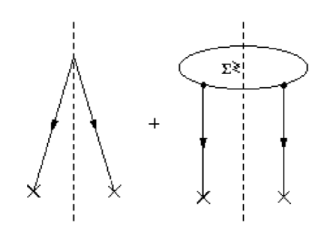
Figure 4: Cut diagram for the particle densities in the Generalized Fluctuation-Dissipation Theorem.

1 Sources

The first step toward getting the phase-space evolution equations from the Generalized Fluctuation-Dissipation Theorem is calculating the self-energies (i.e. the sources). To do this, we insert Equations (27) and (15) into the self-energy equations and keep only the lowest order approximation to the vertex functions. Thus, we assume that the vertices are not dressed and are point-like. So, we arrive at the creation and absorption rates:

$$Q^{\gtrless}(1,1^{\prime})= i\alpha_{em}Z^{2}\stackrel{{\scriptstyle\leftrightarrow}}{{\partial}}_{1\mu}{G}^{\gtrless}\!\left(1,1^{\prime}\right)\stackrel{{\scriptstyle\leftrightarrow}}{{\partial}}_{1^{\prime}\nu}{D}^{\gtrless\mu\nu}\!\left(1,1^{\prime}\right)+Q_{\rm MF}^{\gtrless}(1)\delta^{4}\!\left(1-1^{\prime}\right)$$ (36a)

$$\begin{split}\Pi^{\gtrless}_{\mu\nu}(1,1^{\prime})=&i\alpha_{em}{\rm Tr}\left\{\gamma_{\mu}{S}^{\gtrless}\!\left(1,1^{\prime}\right)\gamma_{\nu}{S}^{\lessgtr}\!\left(1,1^{\prime}\right)\right\}\\ &+i\alpha_{em}Z^{2}\stackrel{{\scriptstyle\leftrightarrow}}{{\partial}}_{1\mu}{G}^{\gtrless}\!\left(1,1^{\prime}\right)\stackrel{{\scriptstyle\leftrightarrow}}{{\partial}}_{1^{\prime}\nu}{G}^{\lessgtr}\!\left(1,1^{\prime}\right)+\Pi_{\rm MF}^{\gtrless}(1)g_{\mu\nu}\delta^{4}\!\left(1-1^{\prime}\right)\end{split}$$ (36b)

$$\Sigma^{\gtrless}_{\alpha\beta}(1,1^{\prime})= -i\alpha_{em}(\gamma_{\mu})_{\alpha\alpha^{\prime}}{S}^{\gtrless}_{\alpha^{\prime}\beta^{\prime}}\!\left(1,1^{\prime}\right)(\gamma_{\nu})_{\beta^{\prime}\beta}{D}^{\gtrless\mu\nu}\!\left(1,1^{\prime}\right)+\Sigma_{\rm MF}^{\gtrless}(1)\delta_{\alpha\beta}\delta^{4}\!\left(1-1^{\prime}\right)$$ (36c)

Here we neglect the second scalar term in the polarization tensor and the second photon term in the scalar self-energy because they enter with a factor $\alpha_{em}^{2}$ which is higher order than the other terms.

The self-energies in (36a)–(36c) can be Wigner transformed. Taking care to integrate the derivative scalar couplings by parts, we arrive at

$$\begin{split}Q^{\gtrless}(x,p)=&i\alpha_{em}Z^{2}\int\frac{{d}^{4}q_{1}}{{(2\pi)}^{4}}\>\frac{{d}^{4}q_{2}}{{(2\pi)}^{4}}\>(q_{1}+q_{2}-i\stackrel{{\scriptstyle\leftrightarrow}}{{\partial}}/2)_{\mu}{G}^{\gtrless}\!\left(x,q_{1}\right)\\ &\times(q_{1}+q_{2}-i\stackrel{{\scriptstyle\leftrightarrow}}{{\partial}}/2)_{\nu}{D}^{\gtrless\mu\nu}\!\left(x,q_{2}\right)(2\pi)^{4}\delta^{4}\!\left(p-(q_{1}+q_{2})\right)+Q_{\rm MF}^{\gtrless}(x)\end{split}$$ (37a)

$$\begin{split}\Pi^{\gtrless}_{\mu\nu}(x,p)=&i\alpha_{em}\int\frac{{d}^{4}q_{1}}{{(2\pi)}^{4}}\>\frac{{d}^{4}q_{2}}{{(2\pi)}^{4}}\>{\rm Tr}\left\{\gamma_{\mu}{S}^{\gtrless}\!\left(x,q_{1}\right)\gamma_{\nu}{S}^{\gtrless}\!\left(x,q_{2}\right)\right\}(2\pi)^{4}\delta^{4}\!\left(p-(q_{1}+q_{2})\right)\\ &+i\alpha_{em}Z^{2}\int\frac{{d}^{4}q_{1}}{{(2\pi)}^{4}}\>\frac{{d}^{4}q_{2}}{{(2\pi)}^{4}}\>(q_{1}+q_{2}+i\stackrel{{\scriptstyle\leftrightarrow}}{{\partial}}/2)_{\mu}{G}^{\gtrless}\!\left(x,q_{1}\right)\\ &\times(q_{1}+q_{2}+i\stackrel{{\scriptstyle\leftrightarrow}}{{\partial}}/2)_{\nu}{G}^{\gtrless}\!\left(x,q_{2}\right)(2\pi)^{4}\delta^{4}\!\left(p-(q_{1}+q_{2})\right)+\Pi_{\rm MF}^{\gtrless}(x)g_{\mu\nu}\end{split}$$ (37b)

$$\begin{split}\Sigma^{\gtrless}_{\alpha\beta}(x,p)=&-i\alpha_{em}(\gamma_{\mu})_{\alpha\alpha^{\prime}}\int\frac{{d}^{4}q_{1}}{{(2\pi)}^{4}}\>\frac{{d}^{4}q_{2}}{{(2\pi)}^{4}}\>{S}^{\gtrless}_{\alpha^{\prime}\beta^{\prime}}\!\left(x,q_{1}\right)(\gamma_{\nu})_{\beta^{\prime}\beta}{D}^{\gtrless\mu\nu}\!\left(x,q_{2}\right)\\ &\times(2\pi)^{4}\delta^{4}\!\left(p-(q_{1}+q_{2})\right)+\Sigma_{\rm MF}^{\gtrless}(x)\delta_{\alpha\beta}\end{split}$$ (37c)

6 QED Evolution Equations

We now insert the phase-space self-energies into the phase-space Generalized Fluctuation-Dissipation theorem and rewrite these equations directly in terms of the particle and antiparticle densities.

$$\begin{split}{g^{\gtrless}}\left(x,p\right)=&\int{d}^{4}y\>\frac{{d}^{4}q_{1}}{{(2\pi)}^{4}}\>\frac{{d}^{4}q_{2}}{{(2\pi)}^{4}}\>{G}^{+}\!\left(x-y,p\right)(2\pi)^{4}\delta^{4}\!\left(p-(q_{1}+q_{2})\right)\\ &\times\alpha_{em}Z^{2}(q_{1}+q_{2}-i\stackrel{{\scriptstyle\leftrightarrow}}{{\partial}}/2)^{\mu}{g^{\gtrless}}\left(y,q_{1}\right)(q_{1}+q_{2}-i\stackrel{{\scriptstyle\leftrightarrow}}{{\partial}}/2)^{\nu}{d^{\gtrless}_{\mu\nu}}\left(y,q_{2}\right)\\ &+\int{d}^{4}y\>{G}^{+}\!\left(x-y,p\right)iQ_{\rm MF}^{\gtrless}(y)\\ &+\lim_{y_{0}\rightarrow-\infty}\int{d}^{3}y\>{G}^{+}\!\left(x-y,p\right){g^{\gtrless}}\left(y,\vec{p}\right)\end{split}$$ (38a)

$$\begin{split}{d^{\gtrless}_{\mu\nu}}\left(x,p\right)=&\int{d}^{4}y\>\frac{{d}^{4}q_{1}}{{(2\pi)}^{4}}\>\frac{{d}^{4}q_{2}}{{(2\pi)}^{4}}\>{D}^{+}_{\mu\nu\mu^{\prime}\nu^{\prime}}\!\left(x-y,p\right)(2\pi)^{4}\delta^{4}\!\left(p-(q_{1}+q_{2})\right)\\ &\times\left\{\alpha_{em}{\rm Tr}\left[\gamma^{\mu^{\prime}}{s^{\gtrless}}\left(y,q_{1}\right)\gamma^{\nu^{\prime}}{s^{\gtrless}}\left(y,q_{2}\right)\right]\right.\\ &+\left.\alpha_{em}Z^{2}(q_{1}+q_{2}+i\stackrel{{\scriptstyle\leftrightarrow}}{{\partial}}/2)^{\mu^{\prime}}{g^{\gtrless}}\left(y,q_{1}\right)(q_{1}+q_{2}+i\stackrel{{\scriptstyle\leftrightarrow}}{{\partial}}/2)^{\nu^{\prime}}{g^{\gtrless}}\left(y,q_{2}\right)\right\}\\ &+\int{d}^{4}y\>{D}^{+}_{\mu\nu\mu^{\prime}\nu^{\prime}}\!\left(x-y,p\right)i\Pi_{\rm MF}^{\gtrless}(y)g^{\mu^{\prime}\nu^{\prime}}\\ &+\lim_{y_{0}\rightarrow-\infty}\int{d}^{3}y\>{D}^{+}_{\mu\nu\mu^{\prime}\nu^{\prime}}\!\left(x-y,p\right){d^{\gtrless\mu^{\prime}\nu^{\prime}}}\left(y,\vec{p}\right)\end{split}$$ (38b)

$$\begin{split}{s^{\gtrless}_{\alpha\beta}}\left(x,p\right)=&\int{d}^{4}y\>\frac{{d}^{4}q_{1}}{{(2\pi)}^{4}}\>\frac{{d}^{4}q_{2}}{{(2\pi)}^{4}}\>{S}^{+}_{\alpha\beta\alpha^{\prime}\beta^{\prime}}\!\left(x-y,p\right)(2\pi)^{4}\delta^{4}\!\left(p-(q_{1}+q_{2})\right)\\ &\times\alpha_{em}(\gamma^{\mu})_{\alpha^{\prime}\alpha^{\prime\prime}}{s^{\gtrless}_{\alpha^{\prime\prime}\beta^{\prime\prime}}}\left(y,q_{1}\right)(\gamma^{\nu})_{\beta^{\prime\prime}\beta^{\prime}}{d^{\gtrless}_{\mu\nu}}\left(y,q_{2}\right)\\ &+\int{d}^{4}y\>{S}^{+}_{\alpha\beta\alpha^{\prime}\beta^{\prime}}\!\left(x-y,p\right)\left(\pm i\Sigma_{\rm MF}^{\gtrless}(y)\right)\delta_{\alpha^{\prime}\beta^{\prime}}\\ &+\lim_{y_{0}\rightarrow-\infty}\int{d}^{3}y\>{S}^{+}_{\alpha\beta\alpha^{\prime}\beta^{\prime}}\!\left(x-y,p\right){s^{\gtrless}_{\alpha^{\prime}\beta^{\prime}}}\left(y,\vec{p}\right).\end{split}$$ (38c)

These equations simultaneously describe all “partonic” splittings, recombinations and scatterings from the distant past to the present. Note that an implementation of these equations would be very different from the conventional transport approach. First, these splittings and recombinations occur in all cells of coordinate space. This is a very different from the conventional approach where particles interact only when they are within $\sqrt{\sigma_{\rm TOT}/\pi}$ of each other [KBH⁺95, KLW87, Gei92a, Gei92b, Gei94, Gei95, Gei96, KOH97]. Because the approach in this thesis is both non-local and Lorentz covariant, implementing it would avoid the causality violating problems implicit in conventional approaches. Second, the particles in our approach do not follow straight-like trajectories. Instead, they have a “probability” distribution for propagating to a certain point. This idea is elaborated on somewhat in the next chapter and discussed in detail in Appendix 5.

Equations (38a)–(38c) are the phase-space QED analog of Mahklin’s evolution equations [Mak95a, Mak95b, MS98]. A QCD version of the phase-space evolution equations should reduce to Makhlin’s equations when integrating out the coordinate dependence. Geiger [Gei96] has derived a set of QCD transport equations based on Makhlin’s work. While his derivation is very similar to our derivation of the phase-space evolution equation, he uses a variant of the Quasi-Classical Approximation tailored toward the DGLAP partons in order to simplify his collision integrals. The QCD version of the transport equations we derive in Section 8 would reduce to his semi-classical equations if one applies this approximation.

There are several ways to solve Equation (38a)–(38c) but we propose only two methods in the following subsections. The first method is a perturbative scheme which we use to derive the time-ordered version of the results of Sections 1–2 in the next chapter. The second method is to derive transport equations from Equations (38a)–(38c).

7 Perturbative Solutions

We can perform a coupling constant expansion on Equations (38a)–(38c) and get the leading contributions to the particle densities. We show this for the photons and electrons surrounding a classical point charge. The discussion here is mainly technical and is designed to show how to perform a perturbative calculation in phase-space. There is an expanded discussion of these densities in the next chapter; there we describe the sources and propagators for the photon and electron densities around a point charge.

We begin by stating the initial densities and listing our assumptions. In the initial state, we assume there is one massive scalar particle serving as the photon source. If we view only photons with a wavelength much larger than the spread of the scalar wavepacket then the scalar particle density is

$${g^{<}}\left(y_{0}=-\infty,\vec{y},\vec{p}\right)={\cal N}\theta(p_{0})\delta^{3}\!\left(\vec{p}-\vec{p_{i}}\right)\delta(p^{2}-M^{2})\delta^{3}\!\left(x_{0}\vec{p}/p_{0}-\vec{x}\right)$$

This form is only needed to make the correspondence between the results here and the results in Chapter 2 and the form is discussed in Appendix 11.C. The initial electron and photon particle densities are all zero:

$${s^{<}_{\alpha\beta}}\left(y_{0}=-\infty,\vec{y},\vec{p}\right)={d^{<}_{\mu\nu}}\left(y_{0}=-\infty,\vec{y},\vec{p}\right)=0$$

Finally, the other assumptions that we make are that we neglect all mean fields and drop the gradients in the scalar-photon coupling.

1 A Photon Distribution

Since the scalar field only couples to the photons, the lowest order contribution to the photon density comes from the photons directly coupling to the initial scalar density. The cut diagram for this process has the form of the left subdiagram in the Generalized Fluctuation-Dissipation theorem of Figure 4 and is shown in Figure 5. In Figure 5, the photon self-energy is the triangular source current loop.

For positive energy photons, we can write down the density directly from Equation (38b):

$$\begin{array}[]{ccl}{d^{<}_{\mu\nu}}\left(x,p\right)&=&\displaystyle\int{d}^{4}y\>\frac{{d}^{4}q_{1}}{{(2\pi)}^{4}}\>\frac{{d}^{4}q_{2}}{{(2\pi)}^{4}}\>{D}^{+}_{\mu\nu\mu^{\prime}\nu^{\prime}}\!\left(x-y,p\right)(2\pi)^{4}\delta^{4}\!\left(p-(q_{1}+q_{2})\right)\\ &&\times\alpha_{em}Z^{2}(q_{1}+q_{2})^{\mu^{\prime}}{g^{<}}\left(y,q_{1}\right)(q_{1}+q_{2})^{\nu^{\prime}}{g^{<}}\left(y,q_{2}\right).\end{array}$$

Now, ${G}^{>}\!\left(x,p\right)={G}^{<}\!\left(x,-p\right)$ because $\gtrless$ propagators obey the relation ${G}^{>}\!\left(x,y\right)={G}^{<}\!\left(y,x\right)$ at lowest order in the coupling. Thus, we can switch one of the ${g^{<}}\left(y,q\right)$ to ${g^{>}}\left(y,-q\right)$, changing it from an initial state antiscalar to a final state scalar (or an initial state hole). Doing so, we have

$$\begin{array}[]{ccl}{d^{<}_{\mu\nu}}\left(x,p\right)&=&\displaystyle\int{d}^{4}y\>\frac{{d}^{4}q_{1}}{{(2\pi)}^{4}}\>\frac{{d}^{4}q_{2}}{{(2\pi)}^{4}}\>{D}^{+}_{\mu\nu\mu^{\prime}\nu^{\prime}}\!\left(x-y,p\right)(2\pi)^{4}\delta^{4}\!\left(p-(q_{1}-q_{2})\right)\\ &&\times\alpha_{em}Z^{2}(q_{1}-q_{2})^{\mu^{\prime}}{g^{<}}\left(y,q_{1}\right)(q_{1}-q_{2})^{\nu^{\prime}}{g^{>}}\left(y,q_{2}\right).\end{array}$$ (39)

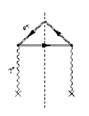
Figure 5: Cut diagram for the time-ordered non-equilibrium photon density.

Comparing Equation (39) and Figure 5 we can further understand the correspondence between the cut diagrams and the perturbative solution. The factor of ${g^{<}}\left(y,q_{1}\right)$ for the initial scalar density is the cut upper double line in Figure 5. The other factor of ${g^{>}}\left(y,q_{2}\right)$ then is the final scalar density and is represented by the lower cut double line.

The entire photon source can be associated with the Wigner transform of the scalar current density after a sum over the final scalar momenta. This is discussed in Appendix 12. Because of this correspondence, Equation (39) is the non-equilibrium, time-ordered, analog of the Wigner transform of the photon vector potential in Section 1.

2 An Electron Distribution

Since the electrons only couple to the photons, the lowest order contribution to the electron density comes from a photon splitting into an electron-positron pair. The cut diagram for this is shown in Figure 6. As one can see, the electron self-energy is everything above the two electron propagators. From Equations (38a)–(38c) we have:

$$\begin{array}[]{ccl}{s^{<}_{\alpha\beta}}\left(x,p\right)&=&\displaystyle\int{d}^{4}y\>\frac{{d}^{4}q_{1}}{{(2\pi)}^{4}}\>\frac{{d}^{4}q_{2}}{{(2\pi)}^{4}}\>{S}^{+}_{\alpha\beta\alpha^{\prime}\beta^{\prime}}\!\left(x-y,p\right)(2\pi)^{4}\delta^{4}\!\left(p-(q_{1}+q_{2})\right)\\ &&\displaystyle\times\alpha_{em}(\gamma^{\mu})_{\alpha^{\prime}\alpha^{\prime\prime}}{s^{<}_{\alpha^{\prime\prime}\beta^{\prime\prime}}}\left(y,q_{1}\right)(\gamma^{\nu})_{\beta^{\prime\prime}\beta^{\prime}}{d^{<}_{\mu\nu}}\left(y,q_{2}\right).\\ \end{array}$$

Using ${s^{<}_{\alpha\beta}}\left(x,q\right)={s^{>}_{\beta\alpha}}\left(x,-q\right)$, we find

$$\begin{array}[]{ccl}{s^{<}_{\alpha\beta}}\left(x,p\right)&=&\displaystyle\int{d}^{4}y\>\frac{{d}^{4}q_{1}}{{(2\pi)}^{4}}\>\frac{{d}^{4}q_{2}}{{(2\pi)}^{4}}\>{S}^{+}_{\alpha\beta\alpha^{\prime}\beta^{\prime}}\!\left(x-y,p\right)(2\pi)^{4}\delta^{4}\!\left(p-(-q_{1}+q_{2})\right)\\ &&\displaystyle\times\alpha_{em}(\gamma^{\mu})_{\alpha^{\prime}\alpha^{\prime\prime}}{s^{>}_{\beta^{\prime\prime}\alpha^{\prime\prime}}}\left(y,q_{1}\right)(\gamma^{\nu})_{\beta^{\prime\prime}\beta^{\prime}}{d^{<}_{\mu\nu}}\left(y,q_{2}\right).\\ \end{array}$$ (40)

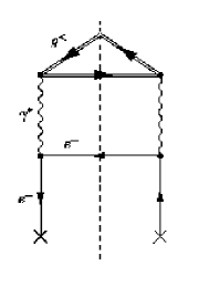
Figure 6: Cut diagram for the time-ordered non-equilibrium electron density.

As with the photon density, this equation maps directly to its analog in Chapter 2, specifically (21). Together the electron density here and the photon density in (39) show that a we can solve the phase-space evolution equations perturbatively.

8 The QED Semi-classical Transport Equations

While we can solve the evolution equations perturbatively, this does not lend itself towards the more complex calculations needed to model a nuclear collision. In this section, we find a set of transport equations from the integral equations in (38a)–(38c). The QCD version of this section might be what is needed to construct a parton transport model. We will find the transport equations by writing two equations of motion for the phase-space retarded propagator. Applying these equations to the phase-space evolution equations, we derive two sets of coupled integro-differential equations. The first set of equations are the transport equations and the second set are the “constraint” equations of Mrówczyński and Heinz [MH94, ZH96]. The transport equations are what is normally solved in a transport approach. The second “constraint” equations, supplement the first by describing the mass shift of the particles in medium.

The equation of motion for the non-interacting retarded massless scalar propagator is

$$\partial^{2}G^{+}(x)=\delta^{4}\!\left(x\right).$$

The conjugate equation is

$$\partial^{2}(G^{+}(x))^{*}=\delta^{4}\!\left(x\right).$$

Multiplying both sides of the first equation by $(G^{+}(y))^{*}$, both sides of the second equation $G^{+}(y)$ and Wigner transforming in the relative space-time coordinate, we find two equations:

$$(k+i\partial/2)^{2}{G}^{+}\!\left(x,k\right)= \int{d}^{4}x^{\prime}\>e^{ix^{\prime}\cdot k}\left(G^{+}(x-x^{\prime}/2)\right)^{*}\delta^{4}\!\left(x+x^{\prime}/2\right)$$ (41a)

$$(k-i\partial/2)^{2}{G}^{+}\!\left(x,k\right)= \int{d}^{4}x^{\prime}\>e^{ix^{\prime}\cdot k}\left(G^{+}(x+x^{\prime}/2)\right)\delta^{4}\!\left(x-x^{\prime}/2\right)$$ (41b)

Inserting the retarded propagator in the energy-momentum representation (with $m_{e}=0$) and adding and subtracting Equations (41a) and (41b), we find the equations of motion for the retarded propagator:

$$k\cdot\partial{G}^{+}\!\left(x,k\right)= \frac{2}{\pi}\theta(x_{0})\delta(x^{2})\sin{(2x\cdot k)}$$ (42a)

$$(\partial^{2}/4-k^{2}){G}^{+}\!\left(x,k\right)= \frac{2}{\pi}\theta(x_{0})\delta(x^{2})\cos{(2x\cdot k)}.$$ (42b)

Taylor series expanding the sine or cosine and keeping only the lowest order is equivalent to performing the gradient expansion in the Quasi-Classical Approximation.

Now, we apply the $k\cdot\partial$ and $(\partial^{2}/4-k^{2})$ operators to the particle densities in Equation (38a)–(38c). On the right hand side, these differential operators act on the retarded propagators, so we can use their equations of motion to simplify the results. For scalars we find

$$\begin{split}\@ADDCLASS{ltx_eqn_lefteqn}$\displaystyle p\cdot\partial{g^{\gtrless}}\left(x,p\right)=\displaystyle\int{d}^{4}y\>\frac{{d}^{4}q_{1}}{{(2\pi)}^{4}}\>\frac{{d}^{4}q_{2}}{{(2\pi)}^{4}}\>\frac{2}{\pi}\theta(x_{0}-y_{0})\delta((x-y)^{2})$\mbox{}\hfil\hskip 18.06749pt\\ &\displaystyle\times\sin{(2(x-y)\cdot p)}(2\pi)^{4}\delta^{4}\!\left(p-(q_{1}+q_{2})\right)\\ &\displaystyle\times\alpha_{em}Z^{2}(q_{1}+q_{2}-i\stackrel{{\scriptstyle\leftrightarrow}}{{\partial}}/2)^{\mu}{g^{\gtrless}}\left(y,q_{1}\right)(q_{1}+q_{2}-i\stackrel{{\scriptstyle\leftrightarrow}}{{\partial}}/2)^{\nu}{d^{\gtrless}_{\mu\nu}}\left(y,q_{2}\right)\\ &+\displaystyle\int{d}^{4}y\>\frac{2}{\pi}\theta(x_{0}-y_{0})\delta((x-y)^{2})\sin{(2(x-y)\cdot p)}iQ_{\rm MF}^{\gtrless}(y)\\ &+\displaystyle\lim_{y_{0}\rightarrow-\infty}\int{d}^{3}y\>\frac{2}{\pi}\theta(x_{0}-y_{0})\delta((x-y)^{2})\sin{(2(x-y)\cdot p)}{g^{\gtrless}}\left(y,\vec{p}\right)\end{split}$$ (43a)

$$\begin{split}\@ADDCLASS{ltx_eqn_lefteqn}$\displaystyle(\partial^{2}/4-k^{2}){g^{\gtrless}}\left(x,p\right)=\displaystyle\int{d}^{4}y\>\frac{{d}^{4}q_{1}}{{(2\pi)}^{4}}\>\frac{{d}^{4}q_{2}}{{(2\pi)}^{4}}\>\frac{2}{\pi}\theta(x_{0}-y_{0})\delta((x-y)^{2})$\mbox{}\hfil\hskip 18.06749pt\\ &\times\displaystyle\cos{(2(x-y)\cdot p)}(2\pi)^{4}\delta^{4}\!\left(p-(q_{1}+q_{2})\right)\\ &\times\displaystyle\alpha_{em}Z^{2}(q_{1}+q_{2}-i\stackrel{{\scriptstyle\leftrightarrow}}{{\partial}}/2)^{\mu}{g^{\gtrless}}\left(y,q_{1}\right)(q_{1}+q_{2}-i\stackrel{{\scriptstyle\leftrightarrow}}{{\partial}}/2)^{\nu}{d^{\gtrless}_{\mu\nu}}\left(y,q_{2}\right)\\ &+\displaystyle\int{d}^{4}y\>\frac{2}{\pi}\theta(x_{0}-y_{0})\delta((x-y)^{2})\cos{(2(x-y)\cdot p)}iQ_{\rm MF}^{\gtrless}(y)\\ &+\displaystyle\lim_{y_{0}\rightarrow-\infty}\int{d}^{3}y\>\frac{2}{\pi}\theta(x_{0}-y_{0})\delta((x-y)^{2})\cos{(2(x-y)\cdot p)}{g^{\gtrless}}\left(y,\vec{p}\right)\end{split}$$ (43b)

Now because of the delta functions, the boundary conditions at $y_{0}\rightarrow-\infty$ only contribute when $|\vec{x}-\vec{y}|$ goes to $\infty$, implying that we need ${g^{\gtrless}}\left(x,p\right)$ as $\vec{x}\rightarrow\infty$. The densities are zero there, so they drop out from these equations.

The transport equations for the photons and electrons are

$$\begin{split}\@ADDCLASS{ltx_eqn_lefteqn}$\displaystyle p\cdot\partial{d^{\gtrless}_{\mu\nu}}\left(x,p\right)=\displaystyle\frac{2}{\pi}\int{d}^{4}y\>\theta(x_{0}-y_{0})\delta((x-y)^{2})\sin{(2(x-y)\cdot p)}$\mbox{}\hfil\hskip 18.06749pt\\ &\times\left\{\displaystyle\int\frac{{d}^{4}q_{1}}{{(2\pi)}^{4}}\>\frac{{d}^{4}q_{2}}{{(2\pi)}^{4}}\>(2\pi)^{4}\delta^{4}\!\left(p-(q_{1}+q_{2})\right)\left\{\alpha_{em}{\rm Tr}\left[\gamma^{\mu}{s^{\gtrless}}\left(y,q_{1}\right)\gamma^{\nu}{s^{\gtrless}}\left(y,q_{2}\right)\right]\right.\right.\\ &+\left.\left.\alpha_{em}Z^{2}(q_{1}+q_{2}+i\stackrel{{\scriptstyle\leftrightarrow}}{{\partial}}/2)^{\mu}{g^{\gtrless}}\left(y,q_{1}\right)(q_{1}+q_{2}+i\stackrel{{\scriptstyle\leftrightarrow}}{{\partial}}/2)^{\nu}{g^{\gtrless}}\left(y,q_{2}\right)\right\}\right.\\ &\left.+g_{\mu\nu}i\Pi_{\rm MF}^{\gtrless}(y)\right\}\end{split}$$ (43c)

$$\begin{split}\@ADDCLASS{ltx_eqn_lefteqn}$\displaystyle p\cdot\partial{s^{\gtrless}_{\alpha\beta}}\left(x,p\right)=\displaystyle\frac{2}{\pi}(\not{\!p}+i\not{\!\partial})_{\alpha\alpha^{\prime}}(\not{\!p}-i\not{\!\partial})_{\beta\beta^{\prime}}$\mbox{}\hfil\hskip 18.06749pt\\ &\times\displaystyle\int{d}^{4}y\>\theta(x_{0}-y_{0})\delta((x-y)^{2})\sin{(2(x-y)\cdot p)}\\ &\times\left\{\displaystyle\int\frac{{d}^{4}q_{1}}{{(2\pi)}^{4}}\>\frac{{d}^{4}q_{2}}{{(2\pi)}^{4}}\>(2\pi)^{4}\delta^{4}\!\left(p-(q_{1}+q_{2})\right)\right.\\ &\times\displaystyle\left.\alpha_{em}(\gamma^{\mu})_{\alpha^{\prime}\alpha^{\prime\prime}}{s^{\gtrless}_{\alpha^{\prime\prime}\beta^{\prime\prime}}}\left(y,q_{1}\right)(\gamma^{\nu})_{\beta^{\prime\prime}\beta^{\prime}}{d^{\gtrless}_{\mu\nu}}\left(y,q_{2}\right)\right.\\ &+\left.\delta_{\alpha^{\prime}\beta^{\prime}}\left(\pm i\Sigma_{\rm MF}^{\gtrless}(y)\right)\right\}.\end{split}$$ (43d)

These equations almost have the form of the Boltzmann equation: the left side clearly is the Boltzmann transport operator and the right side is almost the collision integrals. If we were to expand the sines in the collision integrals and keep only the lowest term, we would recover the collision integrals. Furthermore, if we were to do this same approximation to the QCD version of (43c) we would arrive at Geiger’s semi-classical QCD transport equations [Gei96].

We also state the constraint equations:

$$\begin{split}\@ADDCLASS{ltx_eqn_lefteqn}$\displaystyle(\partial^{2}/4-k^{2}){d^{\gtrless}_{\mu\nu}}\left(x,p\right)=\displaystyle\frac{2}{\pi}\int{d}^{4}y\>\theta(x_{0}-y_{0})\delta((x-y)^{2})\cos{(2(x-y)\cdot p)}$\mbox{}\hfil\hskip 18.06749pt\\ &\times\left\{\displaystyle\int\frac{{d}^{4}q_{1}}{{(2\pi)}^{4}}\>\frac{{d}^{4}q_{2}}{{(2\pi)}^{4}}\>(2\pi)^{4}\delta^{4}\!\left(p-(q_{1}+q_{2})\right)\left\{\alpha_{em}{\rm Tr}\left[\gamma^{\mu}{s^{\gtrless}}\left(y,q_{1}\right)\gamma^{\nu}{s^{\gtrless}}\left(y,q_{2}\right)\right]\right.\right.\\ &+\left.\left.\alpha_{em}Z^{2}(q_{1}+q_{2}+i\stackrel{{\scriptstyle\leftrightarrow}}{{\partial}}/2)^{\mu}{g^{\gtrless}}\left(y,q_{1}\right)(q_{1}+q_{2}+i\stackrel{{\scriptstyle\leftrightarrow}}{{\partial}}/2)^{\nu}{g^{\gtrless}}\left(y,q_{2}\right)\right\}\right.\\ &\left.+g_{\mu\nu}i\Pi_{\rm MF}^{\gtrless}(y)\right\}\end{split}$$ (43e)

$$\begin{split}\@ADDCLASS{ltx_eqn_lefteqn}$\displaystyle(\partial^{2}/4-k^{2}){s^{\gtrless}_{\alpha\beta}}\left(x,p\right)=\displaystyle\frac{2}{\pi}(\not{\!p}+i\not{\!\partial})_{\alpha\alpha^{\prime}}(\not{\!p}-i\not{\!\partial})_{\beta\beta^{\prime}}$\mbox{}\hfil\hskip 18.06749pt\\ &\times\displaystyle\int{d}^{4}y\>\theta(x_{0}-y_{0})\delta((x-y)^{2})\cos{(2(x-y)\cdot p)}\\ &\times\left\{\displaystyle\int\frac{{d}^{4}q_{1}}{{(2\pi)}^{4}}\>\frac{{d}^{4}q_{2}}{{(2\pi)}^{4}}\>(2\pi)^{4}\delta^{4}\!\left(p-(q_{1}+q_{2})\right)\right.\\ &\times\displaystyle\left.\alpha_{em}(\gamma^{\mu})_{\alpha^{\prime}\alpha^{\prime\prime}}{s^{\gtrless}_{\alpha^{\prime\prime}\beta^{\prime\prime}}}\left(y,q_{1}\right)(\gamma^{\nu})_{\beta^{\prime\prime}\beta^{\prime}}{d^{\gtrless}_{\mu\nu}}\left(y,q_{2}\right)\right.\\ &+\left.\delta_{\alpha^{\prime}\beta^{\prime}}\left(\pm i\Sigma_{\rm MF}^{\gtrless}(y)\right)\right\}.\end{split}$$ (43f)

If we were we to derive the constraint equation for massive particles, we would find that $(\partial^{2}/4-k^{2})\rightarrow(\partial^{2}/4-k^{2}+m^{2})$. Therefore, the constraint equations give rise to the in-medium mass shift for the photons and electrons and thus the RHS of the constraint equations for massless particles can be interpreted as an “in-medium” mass. Note that despite the presence of this “in-medium” mass, particles still propagate on the light-cone. Finally, we have not written the various constants in terms of their renormalized values. Dressing the particle densities by solving the evolution equations (which are nonperturbative) should, to some extent, be equivalent to using renormalized couplings.

9 Summary and Implications for QCD Parton Transport Theory

The “source-propagator” picture must apply to QCD partons since the derivation of the phase-space Generalized Fluctuation-Dissipation Theorem does not depend on the form of the self-energies but rather on the form of the Dyson-Schwinger equations for the contour propagators in (22a)–(22c). It would then seem that if we find the QCD self-energies and define the parton distributions appropriately, we may construct QCD phase-space parton evolution equations. However, before we could do this we must assess whether we need to dress the phase-space propagators and vertices and we must implement renormalization.

In the present work, we would dress the particle densities by iterating the phase-space evolution equations but we would not dress the phase-space propagators or vertices. Hopefully, dressing the particle densities is sufficient to incorporate any needed higher order or many particle effects. One simple form of dressing mentioned above is the in-medium mass shift. Given this, it may prove necessary to give particles an effective mass and in this event, we would need the phase-space propagator for non-zero mass. However, we do not know the analytic form of the retarded phase-space propagators for particles with non-zero mass. We are currently investigating propagation in this case and a summary of what we have so far is in Appendix 5.

The issue of implementing renormalization will require some work as there is not a well-developed understanding of renormalization in non-equilibrium quantum mechanics. In momentum-space perturbation theory, renormalization is used to correct some parameters (e.g. a particle’s mass) to make them correspond to their observed values. Some of these corrections can be ascribed to many-particle effects that are effectively dealt with by dressing the densities, propagators and/or vertices. Nevertheless, there may be divergencies that need to be removed in our formulation of non-equilibrium perturbation theory but, at the present, we have not yet encountered any. The issue of renormalization brings up one other question. Usually momentum-space renormalization is interpreted as removing physics at one momentum scale in favor of another scale. It is not clear what this means in phase-space. When renormalizing in phase-space, are we removing physics at a certain length scale, a certain momentum scale, both, or neither? Is renormalization a form of smoothing in phase-space, akin to the gradient approximation?

In any event, these two issues are intricately intertwined and their investigation is beyond the scope of the present work. Nevertheless, in the absence of a phase-space evolution equation, we can still use the Generalized Fluctuation-Dissipation Theorem as insight to build models.

Chapter 2 PARTONS IN PHASE-SPACE

How can we rewrite the QCD Parton Model in phase-space? This is a necessary step if one is to connect the quark and gluon phase-space densities in a transport approach to the Parton Distribution Functions (PDF’s) measured experimentally. Two of the key components of the parton model are factorization of QCD cross sections and evolution of the parton densities. Both of these components can be studied within the Weizsäcker-Williams approximation, the QED analog of the parton model.

Factorization in the QCD Parton Model is the idea that the cross section for a reaction involving a hadron can be written as the convolution of an elementary parton/target cross section and the Parton Distribution Function of the partons in the hadron [AP77, Qui83]. The QED Weizsäcker-Williams approximation follows exactly along this track: a cross section in the Weizsäcker-Williams approximation is the convolution of the Effective Photon Distribution with the elementary photon/target cross section [vW34, Wil34, Jac75, BB88]. We will extend the Weizsäcker-Williams approximation to include electrons. The analogy between the factorization in the parton model and the Weizsäcker-Williams approximation makes even more sense when one realizes that both photons and electrons are the point-like constituents of a dressed QED point charge; in this sense, photons and electrons are the QED partons of the point charge. Thus, by learning how to write the Weizsäcker-Williams Approximation in phase-space, we will be showing factorization in parton model cross sections in phase-space. Now, factorization does fail when there are interference terms in the S-matrix squared and in Appendix 10 we discuss an example the failure of factorization in phase-space. My advisor, Paweł Danielewicz, and I were not the first to consider writing cross sections in phase-space; Remler [Rem90] rewrites transition probabilities in phase-space in his discussion of simulating many-particle systems in phase-space. Remler’s work is not immediately applicable to partons because his work only applies to particles with a large mass.

In the parton model, evolution describes how the the parton densities change via parton splitting and radiation. Evolution is modeled by using evolution equations, which are a set of coupled integro-differential equations for the quark and gluon densities, or by summing over a class of ladder diagrams in the Leading Logarithm Approximation. One such ladder is shown in Figure 7. We can study these ladder diagrams by building up a simplified QED parton ladder. The photon “parton distribution” is the boosted Coulomb field of the point charge and constitutes the first leg in the QED ladder. The electron “parton distribution” is the virtual electron distribution from photons virtually splitting into an electron and a final state positron. The electron is the second leg of the ladder and the positron is the first rung. Since the QED coupling constant, $\alpha_{em}$, is small, only one rung is needed to describe the electron densities and no rungs are needed for the photons. The QCD coupling, $\alpha_{s}$, is much larger implying that a large number of rungs will be needed to reasonably approximate the parton distributions. Thus we can only expect the QED ladder to give some of the qualitative features of the full QCD problem.

Let us outline this chapter. The first two sections, Sections 1 and 2, outline the calculation of the QED phase-space “parton distributions” of a point charge. We begin Section 1 by writing the Weizsäcker-Williams Approximation in phase-space. We do this in several steps. First, we write the reaction rate density for the “partonic subprocess,” namely the reaction rate for absorbing a free photon. By writing this rate in phase-space, we illustrate how we convert a momentum-space reaction rate to one in phase-space. Next, we write the reaction probability for photon exchange in phase-space. Comparing the full reaction probability to the reaction rate density for absorbing a photon, we can identify the phase-space Effective Photon Distribution. This photon distribution is the effective photon number density in phase-space and it has the form of a phase-space source folded with a phase-space propagator. Following this, we calculate the photon number density surrounding a classical point charge and explain how the photon’s phase-space propagator and phase-space source work. Finally, we comment on the implications of this section for the QCD parton model. We will find that we understand how partons propagate, but since our photon source is point-like we do not learn anything about QCD parton sources. In Section 2, we continue the study of the QED parton distributions of a point charge by studying the first link in a parton ladder: a virtual photon splitting into a virtual electron and on-shell positron. We start our analysis by generalizing the phase-space Weizsäcker-Williams Approximation to include electrons and writing down the “Effective Electron Distribution.” This Effective Electron Distribution takes the “source-propagator” form. While this “partonic” splitting leads to a complicated form of the electron source, the shape of the source is mostly determined by the underlying photon (the “parent parton”) distribution. We calculate the electron distribution explicitly for a classical point charge and discuss how the electron propagates from the source to the observation point.

As a practical application of this study, in Section 3 we examine the configuration space structure of the parton cloud of a nucleon. In principle, one should Wigner transform the quark or gluon wavefunctions of a nucleon. Since we do not know the quark or gluon wavefunctions of a nucleon, such a specification is not possible and we must result to model building. One might envision constructing a model phase-space parton density of a nucleon by multiplying the momentum space density (the Parton Distribution Function) and the coordinate space density of the partons [Gei92a, Gei92b, Gei94, GK93, Gei95]. This approximation neglects correlations between the momentum and position in the parton density which are present in the phase-space density [Tat83, Lee95, CZ83]. One might insert these correlations using uncertainty principle based arguments [Mue89, Gei92a, Gei92b, Gei94, GK93, Gei95]. This has intuitive appeal, but such a prescription is ad-hoc at best. We can approach this problem in a more systematic manner using some physical insight from the momentum-space renormalization-group improved parton model and our understanding of how particles propagate in phase-space. In the renormalization-group improved parton model, one calculates the parton densities by evolving the densities in momentum scale, $Q^{2}$ (which we take to be the parton virtuality), and in longitudinal momentum fraction, $x_{F}$. This evolution is equivalent to evaluating a certain class of ladder diagrams and these diagrams can be re-cast in the form of the phase-space Generalized Fluctuation-Dissipation Theorem. Thus, we can discuss the shape of the parton phase-space densities of an hadron in the large-$Q^{2}$ limit or in the small-$x_{F}$ limit using a simple model for the nucleon and the phase-space propagators. We argue that neither large-$Q^{2}$ partons nor small-$x_{F}$ partons extend beyond the nucleon bag in the transverse direction. We also argue that the large-$Q^{2}$ partons extend out an additional $\hbar c/x_{F}P_{L}$ from the bag surface in the longitudinal direction. This is in line with what others have estimated [Mue89, Gei92a, Gei92b, Gei94, GK93, Gei95]. Furthermore, we estimate that the small-$x_{F}$ partons extend at least an additional $\hbar c\sqrt{-q^{2}}$ from the bag so the small-$x$ parton cloud is substantially larger than the large-$Q^{2}$ cloud.

The reaction probabilities that we calculate in this section are for exclusive reactions. The interaction picture Feynman rules for the S-matrix needed for such calculations are found in many field theory books [AB65, BS79, IZ80, Ste93]. The densities we find are directly related to the densities we calculated in the previous chapter by the summation over all final states. This is elaborated on somewhat in Appendix 6 where we discuss measurables of a heavy-ion reaction. Furthermore, we can map our results directly to cross sections in the way outlined in Appendix 7.

1 Photons as QED Partons

If we are to interpret photons as QED partons, we must write the photon exchange process reaction rate in a factorized, parton model-like, form. In other words, we want to write the cross section of the process of photon exchange (pictured in Figure 1(b)) as a convolution of the cross section for free photon absorption (pictured in Figure 1(a)) with an Effective Photon Distribution, and in phase-space. We can then go on to study the properties of the QED version of a phase-space parton distribution with the example of the photon distribution of a point charge. Not only will we rewrite the Weizsäcker-Williams Approximation in phase-space in this work, but we will also show that the phase-space photon density has the form of a phase-space source convoluted with a phase-space propagator. This formal structure of the phase-space densities is a general property as we saw in Chapter 1, so it is not a real surprise to find it here.

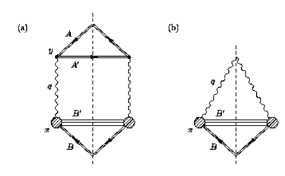
Figure 1: Cut diagrams for photon exchange and free photon absorption. (a) Cut diagram for current A to exchange a photon with current B. (b) Cut diagram for current B to absorb a free photon. In both figures, the photon/current B interaction is unspecified and is represented with a blob.

1 Photon Absorption

We begin this section by finding the photon/current B reaction rate, ${\cal W}_{\rm\gamma B\rightarrow B^{\prime}}$; this reaction rate is our “partonic” subprocess reaction rate. Our derivation demonstrates how to rewrite the reaction probability in terms of phase-space quantities. The high point in this calculation occurs in Equation (1) when we identify the Wigner transforms of B’s current and of the photon field. This type of identification lets us rewrite the reaction probabilities in phase-space.

To find ${\cal W}_{\rm\gamma B\rightarrow B^{\prime}}$ we write the S-matrix for the process in Figure 1(b):

$$S_{\gamma B\rightarrow B^{\prime}} = \int{d}^{4}x\>\left<0\right|A^{\mu}(x)\left|\vec{q},\lambda\right>\left<B^{\prime}\right|j_{\mu}(x)\left|B\right>$$

$$= \int{d}^{4}x\>\frac{{d}^{4}k}{{(2\pi)}^{4}}\>e^{-ik\cdot x}\left<0\right|A^{\mu}(x)\left|\vec{q},\lambda\right>\left<B^{\prime}\right|j_{\mu}(k)\left|B\right>.$$

Here $\left<0\right|A^{\mu}(x)\left|\vec{q},\lambda\right>=\sqrt{\frac{4\pi}{2|q_{0}|V}}\epsilon^{\mu}\!\left(\lambda\right)e^{iq\cdot x}$ is the free photon wave function (with $q^{2}=0$) and $j_{\mu}$ is the current operator for the probe particle B. We leave both the initial and final states of $B$ unspecified so the final state may be a single particle or several particles (as pictured in Figure 1(b)).

If we now square the S-matrix and average over photon polarizations, we find:

$${\left|S_{\rm\gamma B\rightarrow B^{\prime}}\right|}^{2} = \int{d}^{4}x\>{d}^{4}x^{\prime}\>\frac{{d}^{4}k}{{(2\pi)}^{4}}\>\frac{{d}^{4}k^{\prime}}{{(2\pi)}^{4}}\>e^{-i(k\cdot x-k^{\prime}\cdot x^{\prime})}$$

$$\times\displaystyle\frac{1}{2}\sum_{\lambda=\pm}\left<0\right|A^{\mu}(x)\left|\vec{q},\lambda\right>\left<\vec{q},\lambda\right|A^{*\nu}(x^{\prime})\left|0\right>\left<B^{\prime}\right|j_{\mu}(k)\left|B\right>\left<B\right|j^{\dagger}_{\nu}(k^{\prime})\left|B^{\prime}\right>.$$

On writing the coordinates and momenta in terms of the relative and average quantities (i.e. $\tilde{k}=k-k^{\prime}$ and $K=\frac{1}{2}(k+k^{\prime})$), and taking advantage of the momentum conserving delta functions in the current matrix elements, ${\left|S_{\rm\gamma B\rightarrow B^{\prime}}\right|}^{2}$ becomes

$$\begin{split}{\left|S_{\rm\gamma B\rightarrow B^{\prime}}\right|}^{2}=&\int{d}^{4}X\>{d}^{4}\tilde{x}\>\frac{{d}^{4}K}{{(2\pi)}^{4}}\>\frac{{d}^{4}\tilde{k}}{{(2\pi)}^{4}}\>e^{-i(K\cdot\tilde{x}+\tilde{k}\cdot X)}\frac{1}{2}\sum_{\lambda=\pm}\left<0\right|A^{\mu}(X+\tilde{x}/2)\left|\vec{q},\lambda\right>\\ &\times\left<\vec{q},\lambda\right|A^{*\nu}(X-\tilde{x}/2)\left|0\right>\left<B^{\prime}\right|j_{\mu}(K+\tilde{k}/2)\left|B\right>\left<B\right|j^{\dagger}_{\nu}(K-\tilde{k}/2)\left|B^{\prime}\right>.\end{split}$$ (1)

There are two Wigner transforms in this equation: the Wigner transform of the photon field (the $\tilde{x}$ integral) and the Wigner transform of B’s current (the $\tilde{k}$ integral).

Now we rewrite the S-matrix in terms of the phase-space quantities and define the reaction rate density:

$$\begin{array}[]{ccl}\displaystyle{\left|S_{\rm\gamma B\rightarrow B^{\prime}}\right|}^{2}&=&\displaystyle\int{d}^{4}x\>\frac{{d}^{4}k}{{(2\pi)}^{4}}\>\frac{\pi}{V|q_{0}|}\sum_{\lambda=\pm}\epsilon_{\mu}\!\left(\lambda\right)\epsilon^{*}_{\nu}\!\left(\lambda\right)(2\pi)^{4}\delta^{4}\!\left(q-k\right){J}^{\mu\nu}_{\rm B}\!\left(x,k\right)\\ &\equiv&\displaystyle\int{d}^{4}x\>{\cal W}_{\rm\gamma B\rightarrow B^{\prime}}\left(x,q\right).\end{array}$$ (2)

Here the Wigner transform of the current is

$${J}^{\mu\nu}_{\rm B}\!\left(x,q\right)\equiv\int\frac{{d}^{4}\tilde{q}}{{(2\pi)}^{4}}\>e^{-i\tilde{q}\cdot x}\left<B^{\prime}\right|j^{\mu}(q+\tilde{q}/2)\left|B\right>\left<B\right|j^{\dagger\nu}(q-\tilde{q}/2)\left|B^{\prime}\right>.$$ (3)

Since B’s Wigner current is proportional to the reaction rate, it seems natural to give them both the same physical interpretation: as a “probability” density, for absorbing a free photon with momentum $q$ at space-time point $x$. Now, it may not be clear where the spatial structure of the reaction rate comes from, especially since the incident photon is completely delocalized in space (it is in a momentum eigenstate). To give the reaction rate spatial structure, we must localize either the initial or final states of $B$ with a wavepacket.

2 Photon Exchange

We have the probability density,${\cal W}_{\rm\gamma B\rightarrow B^{\prime}}\left(x,q\right)$, for free photon absorption in phase-space. We now need the reaction rate for one-photon exchange (see Figure 1(a)) in phase-space in order to extract the Effective Photon Density. We do it two different ways: in terms of the Wigner transforms of the currents A and B and the photon propagator and in terms of the Wigner transform of the photon vector potential. The first form of the reaction rate has a clear physical interpretation in terms of photon emission, propagation, and absorption. However, it is the second form which can be brought into a factorized form.

The S-matrix for Figure 1(a) is

$$S_{\rm AB\rightarrow A^{\prime}B^{\prime}}=\int d^{4}xd^{4}y\left<A^{\prime}\right|j^{A\mu}(x)\left|A\right>{D}^{\rm c}_{\mu\nu}\!\left(x,y\right)\left<B^{\prime}\right|j^{B\nu}(y)\left|B\right>.$$ (4)

Taking the absolute square of this S-matrix and rewriting it in terms of Wigner transformed currents and propagators, we find

$${\left|S_{\rm AB\rightarrow A^{\prime}B^{\prime}}\right|}^{2}=\int{d}^{4}y\>{d}^{4}x\>\frac{{d}^{4}q}{{(2\pi)}^{4}}\>{J}^{\mu\nu}_{\rm A}\!\left(y,q\right){D}^{\rm c}_{\mu\nu\mu^{\prime}\nu^{\prime}}\!\left(y-x,q\right){J}^{\mu^{\prime}\nu^{\prime}}_{\rm B}\!\left(x,q\right).$$ (5)

Here, the Wigner transform of the photon propagator is

$$\begin{array}[]{ccl}{D}^{\rm c}_{\mu\nu\mu^{\prime}\nu^{\prime}}\!\left(x,q\right)&=&\displaystyle\int{d}^{4}\tilde{x}\>e^{i\tilde{x}\cdot q}D^{c}_{\mu\nu}(x+\tilde{x}/2)D^{c*}_{\mu^{\prime}\nu^{\prime}}(x-\tilde{x}/2)\\ &=&(4\pi)^{2}g_{\mu\nu}g_{\mu^{\prime}\nu^{\prime}}{G}^{\rm c}\!\left(x,q\right)\end{array}$$ (6)

and ${G}^{\rm c}\!\left(x,q\right)$ is the Wigner transform of the scalar Feynman propagator. We outline the derivation and properties of $G^{c}(x,q)$ in Appendix 5.

Equation (5) has an obvious physical meaning: 1) current A makes a photon with momentum $q$ at space-time point $y$, 2) the photon propagates from $y$ to $x$ with momentum $q$ and 3) current B absorbs the photon at space-time point $x$. The spatial structure of the integrand of (5) can come from localizing either $A$ or $B$.

Now we take a detour and calculate the Wigner transform of the vector potential of the current $A$. This detour will lead us to a form of the reaction probability amenable to a parton model-like interpretation. In terms of the current density and propagator, the vector potential with causal boundary conditions is [Jac75]:

$$A^{\mu}(x)=\int{d}^{4}y\>D^{c}_{\mu\nu}(x-y)J_{A}^{\nu}(y).$$ (7)

The Wigner transform of this is:

$$\begin{array}[]{ccl}{A}_{\mu\nu}\!\left(x,q\right)&=&\displaystyle\int{d}^{4}\tilde{x}\>e^{i\tilde{x}\cdot q}A_{\mu}(x+\tilde{x}/2)A_{\nu}^{*}(x-\tilde{x}/2)\\ &=&\displaystyle\int{d}^{4}y\>{J}^{\mu^{\prime}\nu^{\prime}}_{\rm A}\!\left(y,q\right){D}^{\rm c}_{\mu^{\prime}\nu^{\prime}\mu\nu}\!\left(x-y,q\right).\end{array}$$ (8)

The Wigner transform of the vector potential has a “source-propagator” form. Current $A$ (the photon source) creates the photon with momentum $q$ at space-time point $y$ and the propagator takes the photon from $y$ to $x$. Let us put this in Equation (5),

$$|S_{AB\rightarrow A^{\prime}B^{\prime}}|^{2}=\int d^{4}x\frac{d^{4}q}{(2\pi)^{4}}A_{\mu\nu}(x,q)J^{\mu\nu}_{B}(x,q).$$ (9)

Stated this way, the spatial structure of the integrand of this equation comes from either localizing $B$ or from the spatial structure in the Wigner transform of the photon vector potential.

Equation (9) is nearly factorized because current $B$ is proportional to the photon/current B reaction rate and, as we see in the next section, the vector potential is proportional to the phase-space Effective Photon Distribution.

3 The Weizsäcker-Williams Approximation

We have the reaction rate for photon exchange, ${\cal W}_{AB\rightarrow A^{\prime}B^{\prime}}(x,q)$, and the reaction rate for absorption of a free photon, ${\cal W}_{\gamma B\rightarrow B^{\prime}}(x,q)$. Let us compare them and extract the phase-space Effective Photon Distribution. First, we decompose B’s Wigner current into photon polarization vectors, allowing us to rewrite ${\cal W}_{\rm\gamma B\rightarrow B^{\prime}}\left(x,q\right)$ in terms of ${J}^{\mu\nu}_{\rm B}\!\left(x,q\right)$. Knowing this, we can identify the Effective Photon Distribution.

Current Decomposition

If the photon probing ${J}^{\mu\nu}_{\rm B}\!\left(x,q\right)$ is sufficiently delocalized in space (in other words, $\partial_{\sigma}A_{\mu\nu}(x,q)\ll q_{\sigma}A_{\mu\nu}(x,q)$), the momentum-space cutting rules tell us that we can expand ${J}^{\mu\nu}_{\rm B}\!\left(x,q\right)$ in terms of the photon polarization vectors [BGMS75]:

$$\begin{array}[]{ccl}\displaystyle{J}^{\mu\nu}_{\rm B}\!\left(x,q\right)&=&\displaystyle\sum_{\lambda=\pm}\epsilon^{\mu}\!\left(\lambda\right)\epsilon^{*\nu}\!\left(\lambda\right)J_{trans}(x,q)\\ &+&\displaystyle\epsilon^{\mu}\!\left(0\right)\epsilon^{*\nu}\!\left(0\right)J_{scalar}(x,q)\\ &+&\displaystyle\frac{q^{\mu}q^{\nu}}{q^{2}}J_{long}(x,q).\end{array}$$ (10)

Here, $\epsilon_{\mu}(0)$ is the scalar (i.e. time-like) polarization vector: $\epsilon_{\mu}(0)=p_{B\mu}-q_{\mu}q\cdot p_{B}/q^{2}$, where $p_{B}$ is the momentum of B. The transverse polarization vectors, $\epsilon_{\mu}(\pm)$, span the hyperplane perpendicular to $\epsilon_{\mu}(0)$ and $q_{\mu}$. Now, if $A_{\mu\nu}(x,q)$ is not delocalized, then Equation (10) should be modified to include gradients in $x$. However, if we were to include those gradients here, we may not be able to map ${J}^{\mu\nu}_{\rm B}\!\left(x,q\right)$ to ${\cal W}_{\gamma B\rightarrow B^{\prime}}$.

Since $\epsilon^{\mu}\!\left(\lambda\right)\epsilon^{*}_{\mu}\!\left(\lambda^{\prime}\right)=\delta_{\lambda\lambda^{\prime}}$, it is simple to find the separate currents in (10) in terms of ${J}^{\mu\nu}_{\rm B}\!\left(x,q\right)$:

$$J_{scalar}(x,q)=\epsilon_{\mu}\!\left(0\right)\epsilon^{*}_{\nu}\!\left(0\right){J}^{\mu\nu}_{\rm B}\!\left(x,q\right)$$

and

$$J_{trans}(x,q)=\frac{1}{2}\sum_{\lambda=\pm}\epsilon_{\mu}\!\left(\lambda\right)\epsilon^{*}_{\nu}\!\left(\lambda\right){J}^{\mu\nu}_{\rm B}\!\left(x,q\right)$$

The longitudinal piece, $J_{long}(x,q)$, vanishes due to current conservation.

The Effective Photon Distribution

If we insert (10) into Equation (5), the reaction probability is a sum of two terms:

$$\begin{array}[]{ccl}{\left|S_{\rm AB\rightarrow A^{\prime}B^{\prime}}\right|}^{2}&=&\displaystyle\int{d}^{4}x\>\frac{{d}^{4}q}{{(2\pi)}^{4}}\>{A}_{\mu\nu}\!\left(x,q\right)\sum_{\lambda=\pm}\epsilon^{\mu}\!\left(\lambda\right)\epsilon^{*\nu}\!\left(\lambda\right)J_{trans}(x,q)\\ &+&\displaystyle\int{d}^{4}x\>\frac{{d}^{4}q}{{(2\pi)}^{4}}\>{A}_{\mu\nu}\!\left(x,q\right)\epsilon^{\mu}\!\left(0\right)\epsilon^{*\nu}\!\left(0\right)J_{scalar}(x,q).\end{array}$$ (11)

The two terms in (11) describe transverse and scalar photon exchange between currents A and B, respectively.

Noting that if $J_{trans}(x,q)$ has a weak $q^{2}$ dependence, then

$$J_{trans}(x,q)\propto{\cal W}_{\rm\gamma B\rightarrow B^{\prime}}\left(x,q\right).$$

In other words, $J_{trans}(x,q)$ is proportional to the reaction rate for the “partonic” subprocess. Therefore, the transverse term of (11) can be written as

$${\left|S_{\rm AB\rightarrow A^{\prime}B^{\prime}}\right|}^{2}=\frac{1}{4\pi}\int{d}^{4}x\>\frac{Vd^{3}q}{(2\pi)^{3}}\frac{dq^{2}}{2\pi}\frac{dn_{\gamma}\!\left(x,q\right)}{{d}^{3}x\>{d}^{3}q\>dq^{2}}{\cal W}_{\rm\gamma B\rightarrow B^{\prime}}\left(x,q\right),$$ (12)

provided we identify the transverse Effective Photon Distribution as

$$\frac{dn_{\gamma}\!\left(x,q\right)}{{d}^{3}x\>{d}^{3}q\>dq^{2}}=\sum_{\lambda=\pm}\epsilon^{\mu}\!\left(\lambda\right)\epsilon^{*\nu}\!\left(\lambda\right){A}_{\mu\nu}\!\left(x,q\right).$$ (13)

So, Equation (12) generalizes the Weizsäcker-Williams method to phase-space. The Effective Photon Distribution in (13) is the spin summed photon Wigner function. In other words, it is the phase-space number density of photons at time $x_{0}$ per unit $q^{2}$. Now, when we assume that $J_{trans}(x,q)$ has a weak $q^{2}$ dependence we are in essence assuming that the photons are good quasi-particles. We say this for the following reason: since $J_{trans}(x,q)$ is nearly independent of $q^{2}$, we can perform the $q^{2}$ integral in Equation (12) by pulling it past the reaction rate to act solely on the Effective Photon Distribution. In that case, we have

$$\frac{dn_{\gamma}(x,\vec{q})}{{d}^{3}x\>{d}^{3}q\>}=\int\frac{dq^{2}}{2\pi}\frac{dn_{\gamma}\!\left(x,q\right)}{{d}^{3}x\>{d}^{3}q\>dq^{2}}$$

which is the photon quasi-particle density (see Equation (5)). This should not be a surprise since we wanted a photon distribution that we could fold with a reaction rate for on-shell particles. We comment that conventional formulations of the parton model factorization give a similar result for the full parton model cross section: the full parton model cross section is a folding of the Parton Distribution Function (essentially the momentum-space quasi-particle density of partons) with a hard parton cross section (with on-shell parton). While making partons quasi-particles is a questionable goal for transport applications (as partons must be allowed to evolve in $q^{2}$ to properly include many-particle effects), a definition in terms of quasi-particles gives us the connection to the experimentally determined Parton Distribution Functions. Finally, we state that the factorization we have achieved here is possible because their are no interference terms in our expression for the S-matrix squared. In Appendix 10, we explore the case of lepton pair production in the strong electromagnetic field of two passing ions. In that case, there is interference between the photon fields of the two ions and factorization is not possible.

Now, while classical derivations of the Weizsäcker-Williams method begin with finding the photon power spectra from the Poynting flux [Jac75, vW34, Wil34], a quantum mechanical derivation follows along the lines of what we do here [BGMS75, BB88]. Were we to perform the spatial integrals in (11), we would find that the exponentials in the Wigner transforms conspire to make several delta functions. The resulting delta function integrations are trivial and we would quickly recover the momentum-space result.

Finally, we comment that multiplying the photon phase-space density by the projector $\sum_{\lambda=\pm}\epsilon^{\mu}\!\left(\lambda\right)\epsilon^{*\nu}\!\left(\lambda\right)$ in (13) does not render the photon distribution gauge invariant. Were we in momentum space, the projection would render the distribution gauge invariant [BGMS75]. However because we are in phase-space, when we gauge transform ${A}_{\mu\nu}\!\left(x,q\right)$ and apply the projector, terms proportional to $q_{\mu}$ are removed but terms proportional to $\partial/\partial x^{\mu}$ are not. If the distribution is sufficiently delocalized than the gradients in $x$ become negligible and we might find an “approximately” gauge invariant distribution. Of course we could always find a pathological gauge that still makes the result gauge dependent. A truly gauge invariant virtual photon distribution is introduced in Appendix 9. This gauge invariant distribution reduces to (13) when $A_{\mu\nu}(x,q)$ is sufficiently delocalized.

4 The Photon Cloud of a Point Charge

We know we can calculate the QED analog of a phase-space Parton Distribution Function – the phase-space Effective Photon Distribution. The phase-space Effective Photon Distribution is a quasi-particle distribution and the important part of this distribution is the Wigner transform of the vector potential, ${A}_{\mu\nu}\!\left(x,q\right)$. In this section, we calculate $A_{\mu\nu}(x,q)$ for the simple case of a classical point charge radiating photons. If we localize the source’s wavepacket and view it on a length scale larger than its localization scale, we can treat its density as a delta function. In this case, the shape of the photon distribution is determined the photon propagation and we can use this calculation to illustrate how partons propagate in phase-space. Now field theory books tell us we should use the Feynman propagator to propagate the photons, however we will describe photon propagation via the Wigner transform of the retarded (time-ordered) propagator. We will argue that this is a valid procedure and we will summarize the behavior of the propagator. A complete discussion and derivation of the analytic form of the propagator is contained in Appendix 5. As a result of the discussion in the appendix, the photon propagates a distance of roughly $R_{\|}\sim 1/|q_{0}|$ in the direction parallel to its 3-momentum and $R_{\perp}\sim 1/\sqrt{|q^{2}|}$ in the direction perpendicular to its 3-momentum. We demonstrate this behavior by plotting the coordinate-space distribution of photons with $q^{2}\ll q_{0}^{2}$ (making the photons collinear with the source) and with $q^{2}\sim q_{0}^{2}$. In Appendix 8 we examine the additional case of a static point charge (i.e. $\vec{v}=0$). This case is not relevant for QCD partons since a QCD parton source must be taken in the limit $|\vec{v}|\rightarrow c$.

The Photon Source

For our source current, we assume the source particle’s wavepacket is localized on the length scales that the photons can resolve so we can replace the source current with the current of a point particle. The source particle follows a classical trajectory $x_{\mu}=x_{0}v_{\mu}$ with four-velocity $v_{\mu}=(1,v_{L},\vec{0}_{T})$, $v_{L}\approx c$ and $\gamma=1/(1-v_{L}^{2})\gg 1$. Ignoring the recoil caused by photon emission, the current of the point charge is [Jac75]

$$j_{\mu}(x)=ev_{\mu}\>\delta^{3}\!\left(\vec{x}-x_{0}\vec{v}\right).$$

The Wigner transform of this is the classical Wigner current:

$$\begin{array}[]{rl}{J}^{\mu\nu}_{\rm classical}\!\left(x,q\right)&=\displaystyle\int{d}^{4}\tilde{x}\>e^{iq\cdot\tilde{x}}j_{\mu}(x+\tilde{x}/2)j_{\nu}^{\dagger}(x-\tilde{x}/2)\\ &=2\pi\alpha_{em}\>v_{\mu}v_{\nu}\>\delta(q\cdot v)\delta^{3}\!\left(\vec{x}-x_{0}\vec{v}\right).\end{array}$$ (14)

Here $e^{2}=\alpha_{em}$ is the QED coupling constant.

The current has several easy to interpret features. The first delta function sets $q\cdot v=0$. This ensures that the emitted photons are space-like and that current is conserved. It also insures that, when $q^{2}\rightarrow 0$, the photons become collinear with the emitting particle ($q_{0}=v_{L}q_{L}\approx q_{L}$ making $q^{2}\approx{\vec{q_{T}}}^{2}\approx 0$). This delta function arises because we neglect the recoil of the point charge as it emits a photon. The second delta function insures that the source is point-like and follows its classical trajectory.

This source has one other feature of note: it allows for emission of both positive and negative energy photons. In the following work, we consider creating only positive energy photons so we insert a factor of $2\theta(q_{0})$ in (14). This amounts to constraining the source’s initial energy to be greater its final energy.

The Photon Propagator

For the photon propagator, we take the result in Equation (8) and replace the scalar Feynman propagator with the retarded propagator. We have several very good reasons why we can do this. The first is that, in the momentum representation, the retarded propagator and the Feynman propagator are identical for particles with positive energy (normally they differ in their $+i\varepsilon$ prescription). The second is that the Feynman rules for the S-matrix can be formulated equivalently in terms of either propagator [Leh59]. The final reason why we may make this replacement is that one can view Equation (8) as an approximation of Equation (39) where only one exit channel dominates. In Equation (39), the propagator must be retarded by the time-ordering requirements implicit in our discussion in Chapter 1.

Given that the switch is allowed, the scalar part of the retarded phase-space propagator is given in Appendix 5:

$${G}^{+}\!\left(x,p\right)=\frac{1}{\pi}\theta(x_{0})\theta(x^{2})\theta(\lambda^{2})\frac{\sin{(2\sqrt{\lambda^{2}})}}{\sqrt{\lambda^{2}}}$$

Here ${G}^{+}\!\left(x,p\right)$ is the scalar part of the photon propagator, $x$ is the space-time displacement the photon with momentum $q$ traverses and the Lorentz invariant $\lambda^{2}$ is $\lambda^{2}=(x\cdot q)^{2}-x^{2}q^{2}.$ Looking at the equation for ${G}^{+}\!\left(x,p\right)$, there are some obvious features: the photons must propagate inside the light-cone and forward in time. However the rest of the features of the propagator are tied up in the dependence on $\lambda^{2}$. In Appendix 5 (especially Section 1), we go into great detail understanding what this $\lambda^{2}$ dependence means and we will summarize the results here.

Given that our source can only make photons with $q^{2}\leq 0$, we only describe space-like and on-shell propagation. The case of time-like propagation is discussed in the appendix. Now, what we found was that massless particles in phase-space do not follow their classical trajectory. In fact, if we were to characterize their trajectory by the start and end points of the trajectory, then what we found is not a fixed end point at $\vec{x}+\vec{v}\Delta t$, but rather an entire end zone. The size of the zone depends on the virtuality and energy of the photon. This is sketched for photons with space-like momentum in Figure 2. As one can see, the photon can end up anywhere in the end zone; the transverse size of the zone is set by the off-shellness of the photon and the longitudinal size is set by the energy of the photon. For on-shell photons the situation is similar except both the transverse and longitudinal size is set by the energy of the photon. In actual fact, the propagator is a bit more complicated then what we lay out here, but these estimates of the propagation distance will serve us well in understanding the photon density to follow.

Figure 2: A schematic of phase-space propagation for off-shell particles.

The Photon Density

Now we put the photon source and propagator together into the photon density. We concentrate our efforts on $A_{\mu\nu}(x,q)$ because all of the spatial dependence of the photon distribution is tied up in the Wigner transform of the vector potential. Inserting the classical current and the retarded photon propagator in the Lorentz gauge into (8), we find

$${A}_{\mu\nu}\!\left(x,q\right)=4\pi\alpha_{em}\>v_{\mu}v_{\nu}\theta(q_{0})\delta(q\cdot v)\int{d}^{4}y\>{G}^{+}\!\left(x-y,q\right)\>\delta^{3}\!\left(\vec{y}-y_{0}\vec{v}\right).$$ (15)

The delta function integrals in Equation (15) are trivial, however the remaining proper time integral can not be done analytically. We find

$$\begin{split}{A}_{\mu\nu}\!\left(x,q\right)=&\frac{(8\pi)^{2}\alpha_{em}\gamma\theta(q_{0})\delta(q\cdot v)}{\sqrt{-q^{2}}}v_{\mu}v_{\nu}\\ &\times{\cal A}\!\left(2|x\cdot q|,2\sqrt{-q^{2}\gamma^{2}\left((x\cdot v)^{2}-x^{2}v^{2}\right)-(x\cdot q)^{2}}\right),\end{split}$$ (16)

where the dimensionless function ${\cal A}\!\left(a,b\right)$ is given by

$${\cal A}\!\left(a,b\right)=\int_{a}^{\infty}d\tau\frac{\sin{\tau}}{\sqrt{b^{2}+\tau^{2}}}.$$ (17)

There are two interesting cases that are easy to explore: that of photons nearly collinear to the source particle (i.e. $q_{0}\approx q_{L}\gg|\vec{q}_{T}|$), and that of photons with a large transverse momentum (i.e. $|\vec{q}_{T}|\sim q_{0},q_{L}$). Since there is a $1/\sqrt{-q^{2}}$ singularity in the photon density and nearly on-shell photons (i.e. $q^{2}\rightarrow 0$) are collinear, there will be many more collinear photons than any other kind.

Two plots, representative of collinear photons and high $\vec{q}_{T}$ photons, are shown in Figure 3. The left is a plot of the dimensionless function ${\cal A}\!\left(a,b\right)$ for collinear photons with $q_{\mu}=(m_{e},m_{e}/v_{L},\vec{0}_{T})$. On the right is a plot of ${\cal A}\!\left(a,b\right)$ for photons with transverse momentum comparable to their transverse momentum and energy, $q_{\mu}=(m_{e},m_{e}/v_{L},0.56{\rm MeV/c},0)$. The characteristic energy scale of QED is $m_{e}$, so we choose this scale for the momenta to plot. In both plots, we chose $v_{L}=0.9c$ to illustrate the Lorentz contraction of the distribution. The oscillations exhibited by both photon distributions are expected for a Wigner transformed density [Tat83, Lee95, CZ83]. To obtain an equivalent classical distribution, one should smear this distribution over a unit volume of phase-space.

Figure 3: Plots of the photon phase-space density. Both figures are plots of the dimensionless function ${\cal A}$ corresponding to the photon number density of a point charge with 3-velocity $\vec{v}=(v_{L},\vec{0}_{T})$ where $v_{L}=0.9c$. These slices of the phase-space density have $q_{\mu}=(m_{e},m_{e}/v_{L},\vec{0}_{T})$ (left) and $q_{\mu}=(m_{e},m_{e}/v_{L},0.56\mbox{ MeV/c},0)$ (right). In both plots, only the negative and zero contours are labeled. The positive contours increase in increments of $0.25$.

Both cuts through the photon distribution show Lorentz contraction. For the collinear photons, this contraction occurs in the longitudinal direction. We can account for the contraction with the behavior of the retarded propagator. We expect that the width will be $\sim R_{\|}=\hbar c/|q_{0}|$ parallel to $\vec{q}$ and $\sim R_{\perp}=\hbar c/\sqrt{|q^{2}|}$ perpendicular to $\vec{q}$. For the collinear photons, $\vec{q}$ is in the longitudinal direction and $q_{0}=\gamma\sqrt{|q^{2}|}$ so the longitudinal width is $\sim R_{L}=\hbar c/\gamma\sqrt{|q^{2}|}$. In other words, the collinear photon distribution is a “Lorentz contracted onion” centered on the moving point source. The inner layers of this “onion” correspond to higher $|q^{2}|$ photons. However, we must emphasize that the contraction is not due to the movement of the source, but rather due to kinematics of the photon’s creation and the propagation of the photon. To illustrate this point, one only needs to look at the high transverse momentum photons: their distribution is tilted. In the case plotted on the right in Figure 3, the photon momentum points $45^{\circ}$ to the longitudinal direction, coinciding with the tilt of the distribution. Furthermore, the width of the distribution is $\sim R_{\|}=\hbar c/|q_{0}|$ along this tilted axis and $\sim R_{\perp}=\hbar c/\sqrt{|q^{2}|}$ perpendicular to this tilted axis.

5 What the Photons Tell Us about QCD Partons

QCD parton model cross sections can be written in phase-space as a folding of the phase-space Parton Distribution Function with the reaction rate for the partonic sub-process. A phase-space Parton Distribution Functions is the number of quasi-particle partons per unit volume in phase-space. The phase-space Parton Distribution Functions is simply related to the underlying quark and gluon phase-space densities through integration over the off-shellness of the particles. The phase-space Parton Distribution Functions have a “source-propagator” form and possibly may be defined in a gauge invariant manner as discussed in Appendix 9. It may not be necessary to resort to gauge invariant parton distributions however, provided the parton evolution equations are gauge covariant. If the phase-space parton source produces only positive energy partons or if we use time-ordered field theory then the partons propagate from their source using the Wigner transform of the retarded propagator. This retarded propagator propagates off-shell partons up to roughly $R_{\|}=\hbar c/{\rm min}(|q_{0}|,|\vec{q}|)$ parallel to the parton three-momentum and $R_{\perp}=\hbar c/\sqrt{|q^{2}|}$ perpendicular to the parton 3-momentum. Both of these estimates are valid only in frames with $q_{0},\vec{q}\neq 0$. When either $q_{0}=0$ or $\vec{q}=0$, propagation is cut off at $\sim R_{\|,\perp}=\hbar c/\sqrt{|q^{2}|}$. On-shell (i.e. $q^{2}=0$) partons tend to follow their classical trajectory, with deviations from that trajectory of order $1/|q_{0}|$.

Despite what we have learned, we know next to nothing about QCD parton sources in phase-space. We use a point source here while, because of the finite size of the valence quark bag, a nucleon has spatial structure on the length scales of interest. Furthermore, QCD partons radiate other partons making Figure 1a an entire ladder diagram and this alters the source. We gain more insight into the phase-space sources in the next few sections.

2 Electrons as QED Partons

In the QCD parton model, the Parton Distribution Functions can be found by summing a class of ladder diagrams and the simplest of these has only one rung, corresponding to a single partonic splitting. The QED analog of the first rung of such a ladder is shown in Figure 4(a) where we see a virtual photon splitting into an electron-positron pair. Probing the electron distribution spawned by this process occurs in three steps: 1) a virtual photon splits into an electron-positron pair with the positron on-shell, 2) the virtual electron propagates from the splitting point toward the probe particle and 3) the electron interacts with the probe. In step 1, we assume that the leading contribution to the virtual electron distribution comes from photon splitting. We put the positron on-shell in order to sum over its states – thus encapsulating all possible emission contributions to the electon density. We can give the rate for Figure 4(a) a parton-model like form by associating steps 1 and 2 with the “Effective Electron Distribution” and step 3 with the electron/probe reaction rate (see Figure 4(b)).

Let us outline this section. In Subsection 1, we demonstrate that the reaction rate for the virtual electron exchange process in Figure 4(b) factorizes in phase-space. In the process, the electron phase-space density acquires the “source-propagator” form. In Subsection 2, we calculate the electron distribution of a point charge. The electron source shape is determined mostly by the shape of the parent photon distribution. As with the photon distribution, we use the retarded propagator here instead of the Feynman propagator. We assume the electrons are massless throughout this section because quarks in QCD are effectively massless ($\Lambda_{QCD}\sim m_{q}\ll p_{0},|\vec{p}|$). Finally, in Subsection 3 we discuss the implications of this section.

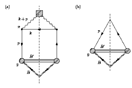
Figure 4: Cut diagrams for a photon splitting into a positron-virtual electron pair and for a free electron interacting with a probe. (a) Cut diagram for creating an electron-positron pair by photon splitting. The virtual electron interacts with the probe particle, $B$. The square vertex represents the photon source. (b) Cut diagram for a free electron interacting with the probe particle.

1 Factorization

First we want to show that the process in Figure 4 can be factorized in phase-space, as needed for a parton model-like form. The S-matrix for the process in Figure 4(a) is:

$$S_{\rm\gamma B\rightarrow\bar{e}B^{\prime}}=\int{d}^{4}x\>{d}^{4}y\>A_{\mu}(x)\psi_{\bar{e}}(x,s)e\gamma^{\mu}S^{c}(x-y){\cal V}_{\rm Be\rightarrow B^{\prime}}(y).$$ (18)

The spatial structure of the electron source comes from localizing the photon vector potential, $A_{\mu}(x)$. The spatial structure of the “partonic” subprocess comes from ${\cal V}_{\rm Be\rightarrow B^{\prime}}(y)$, the electron/probe interaction in Figure 4(b). In Equation (18), $\psi_{\bar{e}}(x,s)=\int\frac{{d}^{4}k}{{(2\pi)}^{4}}\>v(k,s)e^{ik\cdot x}\frac{f^{*}(k)}{\sqrt{2k_{0}V}}$ is the final state positron wavepacket and $S^{c}(x-y)=\int\frac{{d}^{4}p}{{(2\pi)}^{4}}\>e^{-ip\cdot(x-y)}\frac{\not{p}+m_{e}}{p^{2}+m_{e}^{2}+i\epsilon}$ is the electron’s Feynman propagator.

We square $S_{\rm\gamma B\rightarrow\bar{e}B^{\prime}}$ and write it in terms of phase-space quantities:

$$\begin{split}{\left|S_{\rm\gamma B\rightarrow\bar{e}B^{\prime}}\right|}^{2}=&\alpha_{em}\displaystyle\int{d}^{4}x\>{d}^{4}y\>\frac{{d}^{4}p}{{(2\pi)}^{4}}\>\frac{{d}^{4}q}{{(2\pi)}^{4}}\>\frac{{d}^{4}k}{{(2\pi)}^{4}}\>{A}_{\mu\nu}\!\left(x,q\right)f(x,k)\\ &\times(2\pi)^{4}\delta^{4}\!\left(k+p-q\right){\rm Tr}\left\{\frac{1}{2}(\not{\!k}-m)\gamma^{\mu}S^{c}(y-x,p){\cal V}_{\rm Be\rightarrow B^{\prime}}(y,p)\gamma^{\nu}\right\}\end{split}$$ (19)

Here, $S^{c}(y-x,p)$ is the Wigner transform of the two electron Feynman propagators and it can be written in terms of the Wigner transform of the scalar Feynman propagator, ${G}^{\rm c}\!\left(x,q\right)$:

$$\begin{array}[]{rl}{S}^{\rm c}_{\alpha\alpha^{\prime}\beta\beta^{\prime}}\!\left(x,p\right)&=\displaystyle\int\frac{{d}^{4}\tilde{p}}{{(2\pi)}^{4}}\>e^{-i\tilde{p}\cdot x}S^{c}_{\alpha\beta}(p+\tilde{p}/2)\bar{S}^{c}_{\alpha^{\prime}\beta^{\prime}}(p-\tilde{p}/2)\\ &=(\not{\!p}+i\not{\!\partial}+m_{e})_{\alpha\beta}(\not{\!p}-i\not{\!\partial}+m_{e})_{\alpha^{\prime}\beta^{\prime}}{G}^{\rm c}\!\left(x,p\right).\end{array}$$

Also in Equation (19), ${\cal V}_{\rm Be\rightarrow B^{\prime}}(y,p)$ is the Wigner transform of the electron/probe interaction and $f(x,k)$ is the phase-space density of final state positrons.

Now we want to sum over the full set of positron final states. The positron is on-shell and in a momentum eigenstate so we sum over the positron momentum and spin. Furthermore, we can separate off the spinor structure of the electron propagator and shift the derivatives to act on ${\cal V}_{\rm Be\rightarrow B^{\prime}}$. In the end we find

$$\begin{split}{\left|S_{\rm\gamma B\rightarrow\bar{e}B^{\prime}}\right|}^{2}=&\displaystyle\alpha_{em}\int{d}^{4}x\>{d}^{4}y\>\frac{{d}^{4}p}{{(2\pi)}^{4}}\>\frac{{d}^{4}q}{{(2\pi)}^{4}}\>\frac{{d}^{3}k_{f}}{2\left|{k_{f}}_{0}\right|{(2\pi)}^{3}}\>\\ &\displaystyle\times{A}_{\mu\nu}\!\left(x,q\right){G}^{\rm c}\!\left(y-x,p\right)(2\pi)^{4}\delta^{4}\!\left(k_{f}+p-q\right)\\ &\displaystyle\times{\rm Tr}\left\{\frac{1}{2}(\not{\!k}_{f}-m)\gamma^{\mu}(\not{\!p}+i\not{\!\partial}/2+m_{e}){\cal V}_{\rm Be\rightarrow B^{\prime}}(y,p)(\not{\!p}-i\not{\!\partial}/2+m_{e})\gamma^{\nu}\right\}.\end{split}$$ (20)

Since ${\cal V}_{\rm Be\rightarrow B^{\prime}}(y,p)$ is separated from the electron propagator, the reaction probability is factorized. We could explicitly calculate the rate for the partonic subprocess $eB\rightarrow B^{\prime}$, but we are only interested in the shape of the distribution as a function of electron momentum. We can guess the form of the electron density just by looking at Equation (20), without performing the explicit rate density calculation. The electron density is

$$\begin{array}[]{ccl}\displaystyle\frac{dn_{e^{-}}\!\left(y,p\right)}{{d}^{3}y\>{d}^{3}p\>dp^{2}}&\propto&\displaystyle\alpha_{em}\int{d}^{4}x\>{G}^{\rm c}\!\left(y-x,p\right)\int\frac{{d}^{3}k}{2\left|{k}_{0}\right|{(2\pi)}^{3}}\>{A}_{\mu\nu}\!\left(x,k+p\right)\\ &\equiv&\displaystyle\int{d}^{4}x\>{G}^{\rm c}\!\left(y-x,p\right)\Sigma(x,p).\end{array}$$ (21)

Here, ${G}^{\rm c}\!\left(x,p\right)$ is the Wigner transform of the scalar propagator. Equation (21) has the “source-propagator” form: $\Sigma$, the integral of ${A}_{\mu\nu}\!\left(x,k+p\right)$ over the positron momentum, plays the role of the partonic source. Because the emitted positron’s wavepacket has no configuration space structure (it is in a momentum eigenstate), the spatial structure of the source comes solely from the parent photon’s phase-space distribution.

At this stage, we see several important features of the source. First, we note the $d^{3}k/|k_{0}|$ in the positron momentum integral. This factor weights positron emission toward small $k_{0}$ and is the origin of the small–$x_{F}$ singularity used in BFKL evolution [Fie89, D⁺91, SCC95, TW94, LL94]. Second, we note that the entire spatial dependence of the electron source comes from the parent photon distribution. These two points are especially important for the partons in Section 3 so they are elaborated on in the next subsection.

2 The Electron Cloud of a Point Charge

Our main interest is with how the “parton ladder” (in our case, the source is only one rung of the ladder) shapes the electron distribution. First, we discuss the electron’s source and how both the parent photon distribution and the cut positron rung effect it. Second, we discuss the interplay of the electron creation and propagation. Because the electron has positive energy, we can use either the retarded or Feynman phase-space propagator. We choose to use the retarded propagator. We describe the Feynman propagator in Appendix 5.

The Electron Source

In our electron source, we use the photon distribution of Equation (16). This is not a QCD parton-like distribution as the photon source is point-like. Nevertheless, because the electron source is a short parton ladder, it contains many of the general features that one expects from a QCD parton source. In particular it contains the $1/|k_{0}|$ singularity from the integration over final state positrons (in other words, the cut positron rung). We discuss the effects of this integration and we detail both the shape of the source and how this shape depends on the photon distribution.

Up to irrelevant factors, the electron source is

$$\Sigma(x,p)\propto\alpha_{em}\int{d}^{4}k\>\theta(-k_{0})\theta(p_{0}+k_{0})\delta\!\left(k^{2}-m_{e}^{2}\right)\delta\!\left(q\cdot v\right)\frac{{\cal A}\!\left(a,b\right)}{\sqrt{-(k+p)^{2}}}$$ (22)

where $a=2|x\cdot(k+p)|$ and $b=2\sqrt{-(k+p)^{2}\gamma^{2}((x\cdot v)^{2}-x^{2}v^{2})-(x\cdot(k+p))^{2}}$. The longitudinal and temporal positron momentum integrals can be done with the aid of the delta functions, leaving the transverse momentum integrals:

$$\begin{array}[]{rl}\Sigma(x,p)\propto&\displaystyle\alpha_{em}\theta(p\cdot v)\int_{|\vec{k}_{T}|<k_{T{\rm max}}}\frac{{d}^{2}k_{T}\>}{\sqrt{k_{T{\rm max}}^{2}-k_{T}^{2}}}\\ &\times\displaystyle\left\{\frac{\theta(p_{0}+k_{0+}){\cal A}\!\left(a_{+},b_{+}\right)}{\sqrt{-(k_{+}+p)^{2}}}+\frac{\theta(p_{0}+k_{0-}){\cal A}\!\left(a_{-},b_{-}\right)}{\sqrt{-(k_{-}+p)^{2}}}\right\}.\end{array}$$ (23)

Here, $k_{T{\rm max}}^{2}=\gamma^{2}(p\cdot v)^{2}-m_{e}^{2}$ and

$$\begin{array}[]{rcl}k_{0\pm}&=&-\gamma(\gamma p\cdot v\mp v_{L}\sqrt{k_{T{\rm max}}^{2}-\vec{k}_{T}^{2}})\\ k_{L\pm}&=&-\gamma(\gamma v_{L}p\cdot v\mp\sqrt{k_{T{\rm max}}^{2}-\vec{k}_{T}^{2}}).\end{array}$$ (24)

Now, in a parton ladder we expect to find a factor of $d^{3}k/|k_{0}|$ for each cut rung. Here is no exception, one can see that $d^{4}k\theta(-k_{0})\delta(k^{2}-m^{2}_{e})$ gives us this factor. However, because we neglect the recoil of the source, we have an additional $\delta(q\cdot v)$, turning this factor into $d^{2}k/\sqrt{k_{T{\rm max}}^{2}-k_{T}^{2}}$. Because of this factor, the positron’s tend to have $|\vec{k}_{T}|\ll|k_{L}|$, making the positron momentum collinear (or anti-collinear) to the point charge’s velocity. The small photon momentum forces the electron to be emitted with momentum opposite the positrons. Incidentally, one finds this same behavior of the momenta of the leg and rung partons of a real QCD parton ladder. There, the collinearity of the momenta of the partons with the hadron momentum gives rise to the so-called collinear or infra-red singularities.

Now, the shape of $\Sigma$ comes from the parent photon distribution. In our simple case, we can actually estimate the $\left<q_{\mu}\right>$ that gives the dominant contribution to $\Sigma$. For $v_{L}\approx 1$, we estimate that the average $\left<k_{\mp\mu}\right>$ is given by

$$\left<k_{\mp\mu}\right>=\gamma^{2}(p\cdot v)\left(-1\pm\frac{1}{2},-1\pm\frac{1}{2},\cos(\theta_{T})/\gamma,\sin(\theta_{T})/\gamma\right)$$

For the purposes of illustration, we choose to emit the positron in the direction $\hat{k}_{T}\cdot\hat{x}_{T}=\cos(\theta_{T})=\frac{1}{\sqrt{2}}$. By momentum conservation, the dominant photon momentum is $\left<q_{\pm\mu}\right>=p_{\mu}+\left<k_{\pm\mu}\right>$.

On the left in Figure 5, we plot the electron source for $p_{\mu}=(2.0,2.05,\vec{0}_{T})$ MeV/c electrons from a point charge moving to the right with $v_{L}=0.9c$. We choose this $p_{\mu}$ because it is both collinear with the point charge and because it is space-like ($p^{2}<0$). Our source can emit both $p^{2}>0$ and $p^{2}\leq 0$ electrons, however the typical QCD parton in a parton ladder is either space-like or on-shell. On the right in Figure 5, we also plot the photon distribution corresponding to the dominant $\left<q_{\mu}\right>$. Note that both the source and the photon distribution have approximately the same width in both the longitudinal and transverse directions. The tilt in the photon distribution gets averaged away in the $\vec{k}_{T}$ integrals in Equation (23).

Figure 5: Plots of the electron source and underlying photon distribution. On the left:the electron source for electrons with $p_{\mu}=(2.0,2.05,\vec{0}_{T})$ MeV/c. In this figure, only the zero contours are labeled. The positive contours are (in arbitrary units) 1.0, 2.5, 5.0, 7.5 and 10.0. On the right: the virtual photon distributions corresponding to one of dominant contributions to electron source. These photons have a momentum of $\left<q_{+\mu}\right>=(0.956,1.063,0.045,0.045)$ MeV/c. The other root has similar momentum and a similar distribution. In this figure, only the negative and zero contours are labeled. The positive contours increase in increments of 0.25 (in arbitrary units).

The Electron Density

Now we put elements of the electron distribution together. According to Equation (23), we need the Wigner transform of the Feynman propagator. However, since the electrons have positive energy we can replace the Feynman propagator with the retarded propagator as we did for the photons. We discuss both the retarded and Feynman phase-space propagators in Appendix 5.

We are interested in electrons that have momenta that are both space-like and collinear with the source (for comparison with QCD partons), so we plot the coordinate space distribution of electrons with $p_{\mu}=(2.0,2.05,\vec{0}_{T})$ MeV/c in Figure 6. The point source is moving to the right with velocity $0.9c$. Both the source and the underlying photon distribution for these electrons is shown in Figure 5. To perform the four-dimensional spatial integral in Equation (23), we use a Monte-Carlo integration scheme [P⁺92]. This integration scheme, being probabilistic by nature, returns both the integral at a point and the error on the integral at that point. The nonzero data points never had a relative error greater than 20%, but due to this error, the location of the zero contours is uncertain by $\sim 30$ fm.

Figure 6: Coordinate space dependence of the electron phase-space density at four momentum $p_{\mu}=(2.0,2.05,\vec{0})$ MeV/c. Only the negative and zero contours are labeled. The positive contours are in increments of 1.0 (in arbitrary units). The sign of the contours in each region are denoted by $\pm$ signs.

Comparing the electron distribution with the source, we see that the electron distribution is elliptical with longitudinal and transverse widths comparable to what one expects by adding the source width in Figure 5a to the estimates for the propagation distance in Equations (15c). Unlike the electron source distribution, the electron distribution is not symmetric about $x_{L}=0$. This is caused by the positron recoil because, were there no positron recoil, we would have a delta function to insure $p_{0}=p_{L}v_{L}$ (as we found for the photons). Because of the positron recoil, the delta function is widened and the additional spread in energy causes electrons with the chosen momentum to propagate forward preferentially.

3 What the Electrons Tell Us About QCD Partons

In this section, we learned several things about the phase-space densities for massless QCD partons. Owing to the fact that the simplest parton ladder contains one rung representing a single partonic splitting, we learned how both the parent parton and cut rung affect the parton distribution. The shape of the parent parton distribution determines the spatial structure of the parton source. The integral over the final states of the parton represented by the cut rung of the parton ladder has a $1/k_{0}$ weight – giving the parton a low $k_{0}$ (or small longitudinal momentum) and giving rise to the expected collinear singularity.

3 The Parton Cloud of a Nucleon

We cannot calculate the phase-space Parton Distribution Functions without a set of QCD phase-space evolution equations. Although both the work in Chapter 1 and the recent work by Makhlin and Surdutovich [MS98] are steps toward this goal, neither are sufficient. In the renormalization group improved parton model, one specifies the Parton Distribution Functions along some curve in the $x_{F}$-$Q^{2}$ plane and then evolves in $x_{F}$, $Q^{2}$ or both, mapping out the entire PDF for all $x_{F}$ and $Q^{2}$. This evolution is equivalent to summing over a class of ladder diagrams in the Leading Logarithm Approximation. Because the Leading Logarithm Approximation can be translated into phase-space, many of the insights from the Leading Logarithm Approximation in momentum-space can be reused in phase-space. More precisely, using the momentum ordering in the Leading Logarithm Approximation and a simple model of the nucleon we can estimate the size of the sea parton distribution as a function of parton momentum.

1 QCD Parton Model and Leading Logarithm Approximation

Typically the Parton Distribution Functions are calculated using either Dokshitzer-Gribov-Lipatov-Altarelli-Parisi (DGLAP), Balitsky-Fadin-Kurayev-Lipatov (BFKL), or Gribov-Levin-Ryskin (GLR) evolution equations, all of which are equivalent to applying a Leading Logarithm Approximation (LLA) [GLR83, LL94, D⁺91]. In the LLA, we assume the parton is produced in a cascade represented by the ladder diagram in Figure 7. The probability of emitting the $n^{th}$ parton with longitudinal momentum fraction $x_{Fn}$ and transverse momentum $q_{nT}^{2}$ from this cascade goes like [LL94]

$$dP_{n}=\frac{N_{c}\alpha_{s}}{\pi}\frac{dx_{Fn}}{x_{Fn}}\frac{dq_{nT}^{2}}{q_{nT}^{2}}.$$ (25)

Thus, by ordering the momentum properly as we go down the ladder, we can pick up the largest logarithmic contributions to the $n^{th}$ parton’s density.

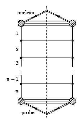
Figure 7: Cut diagram for probing the $n^{th}$ generation of partons in a typical cascade.

Most hadron colliders probe regions where the data are well described with Parton Distribution Functions calculated within the Dokshitzer-Gribov-Lipatov-Altarelli-Parisi (DGLAP) evolution scheme. DGLAP evolution is equivalent the Leading Logarithm Approximation in $1/q^{2}$ (LLA($Q^{2}$)). New experiments at HERA are beginning to see evidence that Balitsky-Fadin-Kurayev-Lipatov (BFKL) type evolution is necessary to describe the Parton Distribution Functions at small-$x_{F}$ [AHC95]. BFKL-type physics is believed to be responsible for the rise in the number of partons as $x_{F}\rightarrow 0$, however this rise can also be partially described by DGLAP-type physics [LL94, NR86, AHC95]. BFKL evolution is equivalent the Leading Logarithm Approximation in $1/x_{F}$ (LLA($x_{F}$)). Unlike DGLAP and BFKL evolution, Gribov-Levin-Ryskin (GLR) type evolution does not have a simple momentum ordering because one sums terms with varying powers of $1/x_{F}$ and $1/q^{2}$ [GLR83, LL94]. Because of the simplicity of the ladder structure and the momentum ordering needed to pick up the largest contributions, we will discuss both DGLAP and BFKL type partons in phase-space.

We can apply the QCD parton model and LLA in phase-space if both are modified appropriately. Assume that we are working in a regime where $\alpha_{s}\ll 1$, so we can apply perturbation theory, and assume that all elementary particles are massless. Assume also that the probe in Figure 7 is localized on the length scale of the parton cloud. This assumption is equivalent to saying the parton lifetime is large compared to the interaction time.

Now, if we find the same singularities in both phase-space and momentum-space, then we know that the LLA will give the dominant contribution to the particle densities in phase-space. From what we have seen from the photon and electron density calculations and from the Generalized Fluctuation Dissipation Theorem, the parton densities have the form

$$f(x,p)=\int{d}^{4}y\>G^{+}(x-y,p)\Sigma(y,p).$$ (26)

The self-energy, $\Sigma$, is given by the parton ladder in Figure 7 and the $n^{th}$ segment of $\Sigma$ is shown in Figure 8. In momentum-space, the cut rung gives a $d^{3}k/|k_{0}|$ which leads to the $dx_{F}/x_{F}$ in Equation (25). To see how the factor of $d^{3}k/|k_{0}|$ arises in phase-space, one needs only look at the electron source in Section 2. The electron source has exactly the form of the segment in Figure 8 and in that calculation we found exactly this factor of $d^{3}k/|k_{0}|$. The fact that we find the same factor of $d^{3}k/|k_{0}|$ in both the energy-momentum representation and in phase-space simply reflects the fact that the cut parton density is proportional to $\theta\!\left(k_{0}\right)\delta(k^{2})$ in both cases and we sum over final parton states. The factor of $dq^{2}/q^{2}$ in Equation (25) comes from the integration over the leg’s propagator, $1/q^{2}$. In phase-space, the $1/q^{2}$ poles are tied up in the Wigner transform of the retarded propagator, but they are still there:

$${G}^{+}\!\left(x,q_{1}-q_{2}\right)=\int\frac{{d}^{4}(q_{1}-q_{2})}{{(2\pi)}^{4}}\>e^{-ix\cdot(q_{1}-q_{2})}\frac{1}{q_{1}^{2}+i\epsilon q_{10}}\frac{1}{q_{2}^{2}-i\epsilon q_{20}}.$$

Thus, this segment of the parton ladder produces the same divergencies in phase-space and momentum-space. Whatever orderings are needed to produce the leading contributions in momentum space will produce the same leading contributions in phase-space.

Figure 8: Typical rung of the LLA ladder.

Our self-energy has the same ladder structure as the electron source in Section 2, so we know the spatial structure of the $n^{th}$ parton’s source is given by the $n-1^{th}$ parton’s distribution. Iterating back to the $0^{th}$ parton (a valence quark), we see that the shape of the valence distribution sets the shape of the sea parton source. So, we take the valence quark wavefunction to be uniformly spread throughout a bag with radius $R_{bag}$ as illustrated in Figure 9. Since we are interested in high-energy collisions, we take the nucleon to be moving to the right with 4-momentum $p_{\mu}=(P_{0},P_{L},\vec{0}_{T})$ with $P_{0}\approx P_{L}\gg M_{N}$. Thus, this nucleon has 4-velocity $v_{\mu}=(1,v_{L},\vec{0}_{T})$ and the bag is contracted in the longitudinal direction by a factor of $\gamma=1/\sqrt{1-v_{L}^{2}}\gg 1$. We assume the partons lose memory of the original valence quark momentum as one goes down the ladder. Thus, any momentum/coordinate correlations in the source function should be washed out by the spatial integrations in Equation (26). One might expect that the sea partons forget the shape of the nucleon bag as well, but we show that the partons cannot propagate far enough from the original source for this to happen.

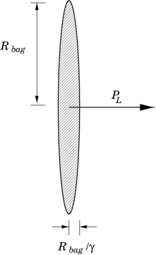
Figure 9: Schematic of the relativistic nucleon’s valence quark distribution.

2 Large-$Q^{2}$ (DGLAP) Partons

In the large-$Q^{2}$ regime, the parton density is low but $\alpha_{s}(Q^{2})\ln(Q^{2}/\Lambda_{QCD}^{2})\gtrsim 1$. Here the largest contribution to the leading log ladder comes from large $Q^{2}$ logarithms. To get the largest contributions from these logs, we order the momenta as we move down the ladder:

$$-q_{n}^{2}\gg-q_{n-1}^{2}\gg\ldots\gg-q_{1}^{2}\gg 1/R^{2}_{bag}\approx\Lambda_{QCD}^{2}.$$

Here $q_{i}^{2}$ is the virtuality of the $i^{th}$ leg. The kinematics at each leg-rung vertex ensure that the momentum fraction carried by each leg is also ordered:

$$1\geq x_{F1}\geq\ldots\geq x_{F{n-1}}\geq x_{Fn}.$$

Whether a rung or leg is a quark or gluon is irrelevant, provided $k^{2}=0$ and the $q^{2}$ ordering holds. Now, given that the proton has longitudinal momentum $P_{L}$ and the rungs and legs are massless, each generation of partons must have energy $q_{n0}\approx x_{Fn}P_{L}$ and transverse momentum of $q_{T}^{2}\approx-q^{2}\ll x_{F}^{2}P_{L}^{2}$.

Let us figure out the general features of the parton cloud. The retarded propagator lets the $n^{th}$ parton propagate out to $R_{n\perp}\sim\hbar c/\sqrt{-q_{n}^{2}}$ transverse to the parton momentum and to $R_{n\|}\sim\hbar c/q_{n0}=\hbar c/x_{Fn}P_{L}$ parallel to the the parton momentum. The parton momentum is approximately parallel to the nucleon momentum, since $x_{F}P_{L}\gg p_{T}$. The partons can never get far from the bag in the transverse direction because $R_{n\perp}\ll R_{bag}$, so the transverse spread of the partons will be dominated by the bag size: $\Delta R_{T}\sim R_{bag}$. On the other hand, the longitudinal spread of the partons is roughly given by $\Delta R_{L}\sim R_{bag}/\gamma+\hbar c/x_{F}P_{L}$, so can be dominated by the longitudinal propagation distance $R_{\|}$ if $x_{F}\ll M_{N}R_{bag}/\hbar c$. In fact, for very small $x_{F}$ (i.e. $x_{F}\sim M_{N}R_{bag}/\gamma\hbar c$) the spread of the partons can meet or exceed the nucleon bag radius. Furthermore, the actual distribution may be somewhat broader due to the propagation of the virtual partons between the subsequent emissions along the ladder.

So in our picture, which is summarized in Figure 10, the sea large-$Q^{2}$ parton distributions have the same transverse size as the parent nucleon’s transverse size, but the longitudinal size can be significantly bigger than the parent’s longitudinal size and even approaching the parent’s transverse size. Furthermore, the drop off in the parton density in the longitudinal direction occurs at the characteristic radius of $\sim\hbar c/x_{F}P_{L}$. This picture of the nucleon is consistent with the uncertainty principle based arguments of A. H. Mueller [Mue89], later user by Geiger to initialize the parton distributions in his Parton Cascade Model [Gei92a, Gei92b, Gei94, GK93, Gei95].

3 Small-$x_{F}$ (BFKL) Partons

In the small-$x_{F}$ regime, the parton density is high and $\alpha_{s}(Q^{2})\ln(1/x_{F})\gtrsim 1$. The small-$x_{F}$ partons are mostly gluons. In this regime, the leading logs come from the $1/x_{F}$-type singularities, i.e. from the cut rungs. Since leading logs come from the $1/x_{F}$ singularities, the largest contributions come about by strongly ordering the longitudinal momentum fraction as one moves down the ladder [BL78, KLF76, KLF77, Lip76]:

$$1\gg x_{F1}\gg\ldots\gg x_{F{n-1}}\gg x_{Fn}.$$

BFKL evolution has only a weak dependence on the virtuality of the partons as we move down the ladder, so we assume $q^{2}$ to be fixed: $q_{n-1}^{2}\approx q_{n}^{2}\gg 1/R_{bag}^{2}$. This does not significantly effect the results of the analysis [BL93].

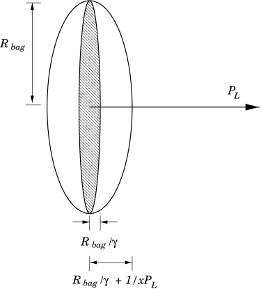
Figure 10: Schematic of the cloud of large $Q^{2}$ partons.

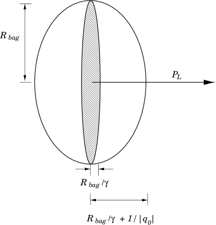
Figure 11: Schematic of the cloud of small $x_{F}$ partons.

Now we must understand how the transverse momentum and energy of each parton leg changes as we go down the ladder. A well known effect of iterating the BFKL kernel (equivalent to moving down the ladder) is that the transverse momentum undergoes a random walk in $\ln(q^{2}_{T})$ [LL94, BL78, KLF76, KLF77, Lip76]. In fact, after iterating through a sufficiently large number of rungs, the spread in the $q_{T}$ distribution is given by:

$$\left<\left(\ln(\frac{q_{nT}^{2}}{q_{1T}^{2}})\right)^{2}\right>=C\ln(\frac{1}{x_{F}})$$

where $C=\frac{N_{c}\alpha_{s}}{\pi}28\zeta(3)=32.14\alpha_{s}$. Thus, $q_{nT}^{2}$ can be orders of magnitude larger or smaller than $q_{1T}^{2}$. This is more clearly seen by rewriting $q_{nT}^{2}$ as

$$q_{nT}^{2}\sim q_{1T}^{2}e^{\pm 5.7\sqrt{\alpha_{s}\ln(1/x_{F})}}.$$ (27)

We will consider the extreme cases of the transverse momentum and comment on the typical case, $q^{2}_{nT}\sim q^{2}_{1T}$.

If the random walk results in a large transverse momentum, we will have $q^{2}_{nT}\gg q^{2}_{1T}\sim-q^{2}\sim(x_{Fn}P_{L})^{2}$. Thus, the $n^{th}$ parton will have 3-momentum in the transverse direction. We know that the parton can only propagate to a distance of roughly $R_{\|}\sim\hbar c/|q_{0}|=\hbar c/\sqrt{q^{2}+q^{2}_{T}+(x_{F}P_{L})^{2}}$ in the direction parallel to $\vec{q}$. Since $\sqrt{q^{2}+q^{2}_{T}+(x_{F}P_{L})^{2}}\approx|q_{T}|$ and $\hbar c/|q_{T}|\ll R_{bag}$, the parton cannot travel far from the original source in the transverse direction. On the other hand, the parton’s longitudinal spread can be larger than the longitudinal bag size. The parton can propagate to a distance of $R_{\perp}\sim\hbar c/\sqrt{-q^{2}}$ in the direction perpendicular to $\vec{q}$, so we can expect a longitudinal spread of the parton distribution of $\Delta R_{L}\sim R_{bag}/\gamma+\hbar c/\sqrt{-q^{2}}$. Since $R_{bag}\gg\hbar c/\sqrt{-q^{2}}$, this additional spread can not match the spread of the DGLAP partons.

If the random walk results in a small transverse momentum, we will have $q^{2}_{nT}\ll q^{2}_{1T}\sim-q^{2}\sim(x_{Fn}P_{L})^{2}$. In this case, the $n^{th}$ parton will have 3-momentum in the longitudinal direction. As in the case of the DGLAP partons the additional transverse spread is $\Delta R_{T}\sim\hbar c/\sqrt{-q^{2}}\ll R_{bag}$ and so is negligible. The additional longitudinal spread is $\Delta R_{L}\sim\hbar c/|q_{0}|\approx\hbar c/\sqrt{q^{2}+(x_{F}P_{L})^{2}}$. This may be significantly larger than the spread of the DGLAP partons because the partons have space-like momenta making $q^{2}+(x_{F}P_{L})^{2}<(x_{F}P_{L})^{2}$.

Summarizing both possibilities, the BFKL parton distribution has a transverse spread of $\Delta R_{T}\sim R_{bag}$, but a widely varying longitudinal spread, ranging from $\Delta R_{L}\sim R_{bag}/\gamma+\hbar c/\sqrt{-q^{2}}\ll R_{bag}$ to $\Delta R_{L}\sim R_{bag}/\gamma+\hbar c/\sqrt{q^{2}+(x_{F}P_{L})^{2}}\gg R_{bag}$ for partons with space-like momentum. Presumably the typical case, when $q^{2}_{nT}\approx q^{2}_{1T}$, lies between these two extremes so the BFKL parton distribution ranges from much smaller than the DGLAP distribution to a lot larger than the DGLAP distribution. In all cases, since $|q_{0}|,\sqrt{-q^{2}},(x_{F}P_{L})\gg\Lambda_{\rm QCD}$, the DGLAP and BFKL distribution longitudinal widths must not be as large as the transverse width. A picture of BFKL partons is illustrated in Figure 11.

The fact that the longitudinal extent of the BFKL cloud can be so much larger than the longitudinal width of the nucleon bag has implications for the small-$x_{F}$ parton distribution of a nucleus. Because the longitudinal width of the small-$x_{F}$ distribution is so large, the small-$x_{F}$ partons (which are mostly gluons) can see the color charge of any other nucleon in a longitudinal tube centered on the parent nucleon. This suggests that we should treat the nucleus as a whole as a source of color charge for the small-$x_{F}$ partons in the spirit of McLerran-Venugopalan model [Ven95]. Specifically, the Lorentz contracted nucleus is replaced with a semi-infinite sheet of fluctuating color charge. In this limit, the gluon distribution function per unit area is the semi-classical Weizsäcker-Williams distribution for gluons scaled by the density of charge squared fluctuation per unit area. In practice in a nuclear collision, this approach may only be useful when the nuclei are far apart. As the nuclei approach, the BFKL partons from each nucleus begin interacting and exciting shorter wavelength modes. These shorter wavelength modes will not see the nuclei as sheets of color charge, but rather objects extended in the longitudinal direction. Eventually then, the McLerran-Venugopalan approach must break down.

The large longitudinal extant of the small-$x_{F}$ cloud may have another consequence: in a zero impact parameter nucleon-nucleon collision, we would find that the soft (BFKL) partons interact much earlier than the harder (DGLAP) partons because of their greater longitudinal spread. This, coupled with the large density of small-$x_{F}$ partons, leads to earlier entropy production and stopping of the soft partons. In fact, this is likely to be part of the cause of the high stopping and early entropy production in the Geiger’s PCM model [Gei92a, Gei92b, Gei94, GK93, Gei95]. However, it is known that small-$x_{F}$ partons couple weakly to themselves and to the rest of the system [McL97, LL94], so this may end up having no observable consequences on the rest of the system.

4 Summary

The parton model rests firmly on the concepts of factorization and on evolution of the parton densities. Using conventional S-matrix perturbation theory on simple QED processes, we showed the reaction rates (and hence the cross sections) can be factorized into a parton model-like form. In other words, they take the form of a reaction rate density convoluted with a phase-space Parton Distribution Function. This phase-space PDF is the quasi-particle parton number density and has the form of a phase-space source folded with a phase-space propagator. Our work with the Weizsäcker-Williams Approximation demonstrates that the Parton Distribution Functions can be defined in phase-space. Since parton evolution is equivalent to summing over a class of ladder diagrams, we examined the first segment of a QED parton ladder. This ladder is simple as it includes only one “partonic” splitting: a virtual photon splitting into an electron-positron pair. Not only does this simple ladder exhibit the $1/x_{F}$ singularity that we would expect from cutting the rung of a parton ladder, but the study of this ladder shows that the shape of a parton’s distribution is controlled to a large extent by the shape of its parent’s distribution.

As a side benefit of this study, we were able to discuss how the phase-space propagators work. We found that the retarded propagator propagates particles to distances of $\sim R_{\|}=\hbar c/\mbox{min}(|q_{0}|,|\vec{q}|)$ parallel to the particle’s momentum and to distances of $\sim R_{\perp}=\hbar c/\sqrt{|q^{2}|}$ perpendicular to the particle’s momentum when $q^{2}\neq 0$. When $q^{2}=0$, the particles tend to follow their classical paths with deviations from this path being of order $1/|q_{0}|$. Furthermore, the retarded propagator can only send particles forward in time and inside the light-cone.

In the end, we have made progress toward specifying the initial phase-space parton distributions of a relativistic nuclear collision. Regardless of the kinematical regime, the transverse spread of a parton distribution is dominated by the bag radius $\sim 1$ fm. The longitudinal spread of a parton distribution varies from roughly $\sim R_{bag}/\gamma+\hbar c/x_{F}P_{L}$ for moderate to large $x_{F}$ (i.e. for DGLAP partons) and from $\Delta R_{L}\sim R_{bag}/\gamma+\hbar c/\sqrt{-q^{2}}$ to $\Delta R_{T}\sim R_{bag}/\gamma+\hbar c/\sqrt{q^{2}+(x_{F}P_{L})^{2}}$ for small $x$ (i.e. BFKL partons). Since the small $x_{F}$ partons have a large longitudinal spread and a high density, we expect the small $x_{F}$ partons to interact much earlier than the large $x_{F}$ partons in a typical nuclear collision. This may cause earlier entropy production and higher stopping than one expects in models that include only DGLAP parton distributions such as HIJING [WG91, WG92, Wan95] and others.

Chapter 3 NUCLEAR IMAGING

Imaging techniques have been applied to a wide variety of problems, from extracting license plate numbers from blurred photos of speeding cars to imaging the interior of the earth. The typical linear imaging problem is to extract an image from experimental data where the data is the convolution of the sought-after image with some kernel. In the study of nuclear reactions we have one such linear imaging problem – inverting the Pratt-Koonin equation:

$$C_{\vec{P}}(\vec{q})-1=\int{d}^{3}r\>K(\vec{q},\vec{r})S_{\vec{P}}(\vec{r}).$$ (1)

Here, the data is the two-particle correlation function, $C$, and the image we seek is the source function, $S$. The source function is the relative distribution of emission points for the pair of particles:

$$S_{\vec{P}}(\vec{r})=\int{d}^{3}R\>dt_{1}dt_{2}D(\vec{P},\vec{R}+\vec{r}/2,t_{1})D(\vec{P},\vec{R}-\vec{r}/2,t_{2}).$$ (2)

Here $D$ is the normalized single particle source and $D$ can be identified with the distribution of last collision points in space, time and momentum of the particles in a nuclear collision. The source function and single particle sources are discussed briefly in Section 1 and in detail in Appendix 6. In (1), the kernel in the convolution is $K(\vec{q},\vec{r})$. For identical pairs, the kernel can be written

$$K(\vec{q},\vec{r})=\left|\phi^{(-)}_{\vec{q}}(\vec{r})\right|^{2}-1.$$ (3)

where, as we discuss in Appendix 6, $\phi^{(-)}_{\vec{q}}(\vec{r})$ is the two particle relative wavefunction. In (1), $\vec{q}$ is the relative momentum between the particle pair, $\vec{r}$ is the separation of emission points in the pair rest frame and $\vec{P}$ is the total pair momentum.

At first glance, imaging appears easy: we could discretize $C_{\vec{P}}$ and $S_{\vec{P}}$ and invert the resulting matrix equation. However, in practice this does not work as small variations in data, even within statistical or systematic errors, can generate huge changes in the reconstructed source. This stability problem is well known in other fields and vast literature exists on its resolution [B⁺85, SG85b, P⁺92, Bal80, BG67]. In fact, many imaging problems [B⁺80, P⁺92] that are now routinely solved would be considered ill-posed in the sense of Hadamard who discussed stability in inversion as early as 1923 [Had23]. One would think then that we could take a well known imaging method, such as the Maximum Entropy Method (MEM) which is often used in astronomical imaging [SG85a, Bev85, P⁺92], and apply it directly to our case. MEM assumes the most likely image on large length scales, corresponding to small amplitude noise, and uses that information to stabilize the image on the shorter length scales, corresponding to the point-like stars. MEM is very successfully applied to astronomical problems but it is not an appropriate approach for nuclear imaging. The reason is that the kernels often encountered by astronomers mainly blur the stars, mixing them into uniform noisy background. In short, the data is rather singular and the kernel is smooth. In our case, the situation is quite the opposite; the source in (1) is highly peaked at small to intermediate distances and drops to zero only at high distances and the kernel is more like a Fourier transform than a blurring function. In other words, our kernel is singular while our data is smooth. In fact, when the kernel does blur, we tend to lose a lot of information.

Given our unique situation, we have tried a variety of techniques to invert (1). These techniques have been applied mainly to the angle-averaged Pratt-Koonin equation and the techniques are discussed in the Section 2. These techniques vary from directly Fourier Transforming the correlation function to more sophisticated methods that seek to arrive at “most likely” source. These more sophisticated methods include the Lucy-Richardson algorithm, where we seek the “most likely” source through an iterative scheme, and others that take the “most likely” source to be the source that minimizes the $\chi^{2}$ fit to the correlation function. These last methods include brute force minimization of the $\chi^{2}$, solving an algebraic equation for the source that produces the smallest $\chi^{2}$, and an improvement of this method we term Optimized Discretization. The most successful of these techniques take advantage of specific properties of either the kernel or the data. In all cases, if we exploit certain properties of the images, i.e. use constraints, we can further stabilize the imaging. Use of constraints implies discarding spurious solutions not meeting the criteria for a valid source. The use of constraints in this role was first recognized by Tikhonov [Tik63] and we will illustrate the use of constraints in the Section 2.

While the images we obtain are interesting in their own right, we will discuss how other pieces of information can be extracted from them in Sections 4 and 3. In particular, we can estimate both the average phase-space density at freeze-out and the entropy of the system at freeze-out from the images. In the past, the average pion phase-space distribution at freeze-out has been estimated using the correlation function [Ber94, Ber96]. However, because we use the source function directly we can make the estimate for any type of particle. There is another piece of information one can extract from the images – the integral of the source over space out to a specific distance. Given that the source function is normalized to 1, if we integrate the source out to a set distance and do not get 1, then we know that a certain amount of the source must lie at greater distances. Since our images can not extend out indefinitely, we can use this quantity to signal for large distance (or long time) emission of pairs we can not otherwise image.

Our imaging work has already yielded an array of new results as we have inverted several data sets from the AGS experiment E877 and from the Michigan State Cyclotron. The results of these inversions are contained in Sections 5, 6 and 7. From the AGS, we analyzed both pion correlations at two different beam energies and kaons at the highest of those two beam energies. Our analysis shows that the kaon source is much narrower than the two pion sources and that the pion sources show evidence for a tail, possibly from long-lived resonance decay. While the pion and kaon sources we found are consistent with Gaussian sources, both the proton and IMF sources are definitely non-Gaussian. We also see clear emission lifetime effects in the sources of both IMF and proton correlations at MSU energies. While we expect that lifetime effects dominate the IMF sources, it was a surprise to see evidence for a tail in the proton sources. In all cases, our imaging allow us to test the positivity of the sources, a condition necessary to interpret the sources semi-classically.

1 What Is the Source Function?

To understand what the images will tell us, we must understand what the source function is, what the source function is not and the coordinates we use to express the source function.

The source function is the probability distribution for emitting a particle pair a distance $\vec{r}$ from one another, in the pairs center of mass frame. First, because it is a probability distribution, if we sum over all possible emission points, then we must obtain 1:

$$\int{d}^{3}r\>S_{\vec{P}}(\vec{r})=1.$$

This will prove useful in our discussion in Section 3. Second, the source says nothing directly about the time separation between the particle emissions. This is clearly seen in Equation (2) as the temporal information in the single particle sources is integrated over. As a specific example of this problem, we can not distinguish between the two scenarios pictured in Figure 1: simultaneous emission with a pair separation $\vec{r}$ and sequential emission with a time separation $\Delta t$ combined with a spatial separation $\vec{r_{0}}$ in a model independent way, if $\vec{r}=\vec{r_{0}}+\vec{v}\Delta t$. The fact that the temporal information is entangled into the source function in such a nontrivial manner cast some doubt on efforts to simultaneously fit the radius of a source function and an effective emission time. Finally, the source is model independent. The only assumption that goes into the inversion process is an assumption of the validity of the Pratt-Koonin equation. In other words, we only require a factorization of final state interactions of the pair from the evolution of the pair in the excited, colliding, nuclear system.

Figure 1: Two emission scenarios that give the same separation of emission points. On the left, the pair is emitted simultaneously with a relative separation $\vec{r}$. On the right, the first particle is emitted with a relative velocity $\vec{v}$ and the second particle is emitted $\Delta t$ later a distance of $\vec{r_{0}}$ from the first particle. The combined spatio-temporal separation of emission is $\vec{r}=\vec{r_{0}}+\vec{v}\Delta t$, giving a separation identical to that in the scenario on the left.

The source function must not be confused with the single particle sources, $D(\vec{x},t,\vec{p})$. However, the source function and single particle sources are related through Equation (2). The single particle sources tell us where and with what momentum the particle are created relative to the system as a whole. The source function can not tell us where either of the particles are created, just how far apart they were when the second one was emitted. Nevertheless, because the source can be written in terms of the single particle sources, model source functions can be constructed from any transport model that gives the distribution of the last collision points in space, time and momentum of the particles in the collision.

The source function is given in the pair center of mass frame in the coordinates sketched in Figure 2. We use the coordinates in Figure 2 as they are commonly used in the analysis of correlation data. We use the CM frame of the pair to simplify the form of the Pratt-Koonin equation. In an arbitrary frame, the source function obtains a dependence on the separation time of the pair emission. This might appear to aid in unfolding the temporal structure of pair emission, but this time dependence is folded into the spatial separation in the $\vec{P}$ direction in a non-trivial manner. In the end, the Pratt-Koonin equation says nothing more than it does in the CM frame, it just does so in a more complicated way.

Figure 2: The directions we use in the analysis of $S$ in the pair center of mass frame are outward along the transverse momentum of the pair, longitudinal along the beam, and the remaining direction we term transverse.

2 Restoring the Source Function

There are several ways that we can approach our imaging problem and in this section we will discuss each of the ones we have considered. These ways range from the simplest Fourier inversion, which is only applicable to particles with no final state interactions, to more sophisticated methods that seek the “most likely” source. The first of these other methods is an iterative scheme called the Lucy-Richardson algorithm. In this scheme the “most likely” source is one that minimizes a quantity similar to the information entropy. The rest of our methods are based on Bayesian arguments that suggest the “most likely” source is one that minimizes the $\chi^{2}$ fit. The least sophisticated (and least successful) of these is the brute force minimization of the $\chi^{2}$. A more fruitful approach is to create an algebraic solution for the $\chi^{2}$ minimum. Now, none of these approaches use any features of the data or kernel to stabilize the inversion. As we will see, our most promising method, the Optimized Discretization method, uses the error on the data and the behavior of the kernel to choose the resolution that produces the best source. One can go further than just taking advantage of the kernel to taking advantage of known properties of the source itself. We describe some of these properties and then use them to further constrain the inversion. We demonstrate the role these constraints have with an example. However, before discussing the various methods, we will recast our inversion problem into the angle-averaged version of the problem.

1 The Angle-Averaged Pratt-Koonin Equation

To begin, we write the angle averaged version of the Pratt-Koonin equation as this is the version we use in the data analysis at the end of the chapter. Although we stick to angle averaged work throughout this chapter, our results are applicable to the full three dimensional case.

If we introduce $C(\vec{q})=\sqrt{4\pi}\sum_{\ell m}C^{\ell m}(q)\,{\rm Y}^{\ell m}(\Omega_{\vec{q}})$, and an analogous representation for $S$ then the individual moments satisfy

$$C_{\vec{P}}^{\ell m}(q)-\delta^{\ell 0}\,\delta^{m0}=4\pi\int_{0}^{\infty}dr\,r^{2}\,K_{\ell}(q,r)\,S_{\vec{P}}^{\ell m}(r)\,.$$ (4)

Here the spin-averaged kernel $K$ depends only on the angle between $\vec{q}$ and $\vec{r}$, and not on the separate directions of these vectors:

$$K_{\ell}(q,r)=\frac{1}{2}\int^{1}_{-1}d(\cos\theta)K(\vec{q},\vec{r})P^{\ell}(\cos\theta).$$ (5)

Due to the symmetry of $S$ and $C$, only even $\ell$ appear in the angular expansion of these functions. Since both functions are real, the moments satisfy $(C^{\ell m})^{*}=(-1)^{m}\,C^{\ell\,-m}$. The relation between the angular moments in (4) may help in analyzing three-dimensional data.

As a specific case, relation (4) shows that the angle-averaged correlation function $C^{00}(q)\equiv C(q)$ is directly related to the angle-averaged source $S^{00}(r)\equiv S(r)$:

$$C_{\vec{P}}(q)-1\equiv{\cal R}_{\vec{P}}(q)=4\pi\int_{0}^{\infty}d{r}\,r^{2}\,K(q,r)\,S_{\vec{P}}(r)\,.$$ (6)

2 Fourier Transformation

One way to invert (6) or (1) is to take advantage of the fact that, when final state interactions can be neglected, the imaging problem becomes a Fourier inversion problem. This means that our intuition regarding Fourier transforms can be applied to the imaging problem.

When we can neglect the final state interactions, the relative wavefunction simplifies dramatically. In particular, for like-charged pions emitted from small sources, their relative Coulomb wavefunction factorizes [PCZ90]:

$$\left|\phi^{\rm Coul}_{\vec{q}}(\vec{r})\right|^{2}\approx G^{2}(q)\left|\phi^{\rm free}_{\vec{q}}(\vec{r})\right|^{2}$$

where

$$G(q)=\frac{2\pi\eta}{e^{2\pi\eta}-1}\quad\text{ and }\quad\eta=\frac{\alpha_{em}m_{\pi}}{2q}$$

and the free wavefunction in the pair rest frame is $\phi^{\rm free}_{\vec{q}}(\vec{r})=(\sqrt{2})^{-1}(e^{i\vec{r}\cdot\vec{q}}+e^{-i\vec{r}\cdot\vec{q}})$. Thus, the Coulomb effects can be “corrected” by dividing out the Gamow factor $G^{2}(q)$ and the inversion becomes a Fourier cosine transform:

$$S_{\vec{P}}(\vec{r})={1\over\pi^{3}}\int{d}^{3}q\>\,\cos{\left(2{\vec{q}\cdot\vec{r}}\right)}\left(C_{\vec{P}}(\vec{q})-1\right)\,.$$ (7)

The angle averaged case follows just as simply as $K(q,r)=\sin{(2qr)}/(2qr)$ and the source, $S_{\vec{P}}$, is an inverse Fourier sine transform of $C$ [BD97]. For the angle-averaged source one finds:

$$r\,S_{\vec{P}}(r)={2\over\pi^{2}}\,\int_{0}^{\infty}dq\,q\,\sin{(2qr)}\,(C_{\vec{P}}(q)-1)\,.$$ (8)

In fact, for any $\ell m$, we have

$$S_{\vec{P}}^{\ell m}(r)={(-1)^{\ell/2}\,4\over\pi^{2}}\int_{0}^{\infty}dq\,q^{2}\ j_{\ell}(2qr)\,(C_{\vec{P}}^{\ell m}(r)-\delta^{\ell 0}\,\delta^{m0})\,.$$ (9)

In practice, the integration in (8) must be cut off at some suitably chosen value of $q_{\rm max}$. This upper limit must be chosen so that the integral covers the region where the correlation in (6) is dominated by the two-particle interference. The magnitude of this cut-off determines the smallest feature that we can resolve in the source. This happens because a feature of size $\Delta r$ will contribute maximally to Fourier modes with frequency $\sim 1/\Delta r$. If the maximum mode one restores has frequency $q_{\rm max}$ then the smallest feature that can be resolved has size $\sim 1/2q_{\rm max}$. Similarly, since the data is typically binned in relative momentum with size $\Delta q$, the source can only be imaged to a distance of $~{}1/\Delta q$.

We will demonstrate the application of Fourier inversion on a two pion correlation function in Section 5. Despite the simplicity of this approach, it does suffer from some problems. First, it only works for cases where the final state interactions can be neglected. This means that it can only really apply to pion and photon correlations. In fact its application to pions is limited to the class of reactions where the source is small. For larger sources, typically a “finite size Coulomb correction” is used, wherein instead of dividing by the Gamow factor, one divides the correlation function by the square of the Coulomb wavefunction smoothed over a finite size Gaussian. It is doubtful that such a correction does anything more than confuse the analysis. Second, Fourier inversion is very sensitive to noise in the correlation function. Simply put, a bump around a specific relative momentum $q_{0}$ appears as a standing wave of frequency $q_{0}$ in the imaged source. This can lead to nonsensical behavior in the tails of the source where the sources amplitude is comparable to the magnitude of the standing wave. Together these problems lead us to consider more sophisticated approaches to imaging the source function.

3 General Case

Typically in an experiment, the correlation function $C_{\vec{P}}$ is determined at discrete values of the magnitude of relative momentum $\{q_{i}\}_{i=1,\ldots,M}$ for directionally-averaged function, or on a mesh in the momentum space $\{\vec{q}_{i}\}_{i=1,\ldots,M}$ when no averaging is done. With each determined value $C_{i}^{\rm exp}$ some error $\Delta C_{i}$ is associated. It is this set of values $\{C_{i}^{\rm exp}\}_{i=1,\ldots,M}$, that we use in determining the source function. In the 3-dimensional case we may introduce a rectangular mesh in the space of relative particle separation and assume that the source function is approximately constant within different cells of the mesh. In the angular expansion (4), we may also assume that the spherical expansion coefficients vary slowly within the $r$-intervals. In the angle-averaged case, discretization amounts simply to the representation $S\simeq\sum_{j=1}^{N}S_{j}\,g_{j}(r)$, where $N$ is the number of intervals in $r$, $g_{j}(r)=1$ for $r_{j-1}<r<r_{j}$, and $g_{j}(r)=0$ otherwise, with $r_{j}=j\,\Delta r$. On inserting a discretized form of $S$ into Equation (1) or (6), we find a set of equations for the correlation functions $\{C_{i}^{\rm th}\}_{i=1,\ldots,M}$, in terms of $\{S_{j}\}_{j=1,\ldots,N}$,

$$C_{i}^{\rm th}-1\equiv{\cal R}_{i}^{\rm th}=\sum_{j=1}^{N}K_{ij}\,S_{j}\,,$$ (10)

where, in the angle-averaged case,

$$K_{ij}=4\pi\int_{r_{j-1}}^{r_{j}}dr\,r^{2}\,K(q_{i},r)\,.$$ (11)

Now, supposing that the correlation function was measured with high accuracy (i.e. that the experimental uncertainties are negligible compared to the data) and that the data do not contain a noise component, the Equation (10) can be inverted using standard Maximum Likelihood methods such as the Lucy-Richardson algorithm. In this method, the source is found through the iteration of the equation [VL93]

$$S^{n}_{j}=\frac{S^{n-1}_{j}}{\sum_{i}K_{ij}}\sum_{i}K_{ij}\frac{C_{i}^{0}}{C_{i}^{n}}$$ (12)

where

$$C_{i}^{n}=\sum_{j}K_{ij}S^{n-1}_{j}$$ (13)

and $S^{0}_{j}$ is an initial guess for the source and $C^{0}_{i}$ is the correlation data. One can see that when the $n^{\rm th}$ iteration generates a source close to the correct one, then $C_{i}^{n}\approx C_{i}^{0}$ making $S_{j}^{n}\approx S_{j}^{n-1}$. So in this method, the “most likely” source is the end result of this iteration and should be close to the true source in the sense of the Kullbeck-Leibler information divergence [VL93]:

$$\sum_{j}S^{\rm true}_{j}\log{(S^{\rm true}_{j}/S^{n}_{j})}$$

This method is general but the convergence is very slow. Furthermore it relies on the notion of highly accurate data, which is often not the case in practice. Finally, it is difficult to implement constraints or to estimate the error in the imaged sources. Luckily images of comparable or better quality can be achieved in much shorter times using the Optimized Discretization method discussed below.

We now adopt a more Bayesian outlook and take the “most likely” source to be the one that has the highest probability given the correlation data. For Gaussian distributed errors, the probability density for $S$ to be the “most likely” source of $C$ is [P⁺92, D’A95]

$$f(S|C)\propto\exp{(-\frac{1}{2}\chi^{2})}$$ (14)

where the $\chi^{2}$ is given by

$$\chi^{2}=\sum_{i=1}^{M}\frac{(C_{i}^{\rm th}-C_{i}^{\rm exp})^{2}}{\Delta^{2}C_{i}}={\rm min}\,.$$ (15)

Clearly the probability density is largest when the source gives the minimum $\chi^{2}$. We can adjust the probability density in (14) by adding factors representing a priori knowledge of the source. For example, if we knew that the source is positive, we could add a factor of $\prod_{j}\theta{(S_{j})}$ to the probability density. The addition of factors such as this, which encode prior knowledge of the source, lead to constraints and the discussion in Subsection 5.

At this point, the obvious thing to do is to search the $\chi^{2}$ surface for a minimum by varying the values of the source function in Equation (10). This is in fact the very first thing we tried however there are problems with this method. In a typical inversion, the source function has roughly 10-15 points so the search for a minimum $\chi^{2}$ takes place over a 10–15 dimensional parameter space. This makes the method slow. Furthermore, in a typical search, one is not always sure the minimum one finds is a true minimum or just a local minimum. This means there is a chance that any solution found is spurious.

Instead, we look for an algebraic way to find the source that minimizes the $\chi^{2}$. If we do not constrain the space within which we search for $\{S_{j}\}_{j=1,\ldots,N}$, then we can get a set of linear equations for the values by functionally differentiating (15) with respect to $\{S_{j}\}_{j=1,\ldots,N}$,

$$\sum_{ij}\frac{1}{\Delta^{2}C_{i}}\left(K_{ij}\,S_{j}-{\cal R}_{i}^{\rm exp}\right)K_{ik}=0\,,$$ (16)

or in a matrix form

$$K^{\top}\,B\,(K\,S-{\cal R}^{\rm exp})=0\,,$$ (17)

where $B_{il}=\delta_{il}/\Delta^{2}C_{i}$. This matrix equation can be solved for $S$:

$$S=\left(K^{\top}\,B\,K\right)^{-1}\,K^{\top}\,B\,{\cal R}^{\rm exp}\,.$$ (18)

So, in Equation (18) we have an algebraic equation for the source function and a new method for determining the source. In the following subsections, we will examine this method and its enhancement, the Optimized Discretization method.

We can determine the error on the source function by applying standard methods of error propagation to (18),

$$\Delta^{2}S_{j}=\left(K^{\top}\,B\,K\right)^{-1}_{jj}\,.$$ (19)

The $N\times N$ matrix $K^{\top}\,B\,K$ in (18) is symmetric, positive definite and may be diagonalized,

$$\left(K^{\top}\,B\,K\right)_{kj}\equiv\sum_{i=1}^{M}\frac{1}{\Delta^{2}C_{i}}\,K_{ik}\,K_{ij}=\sum_{\alpha=1}^{N}\lambda_{\alpha}\,u_{i}^{\alpha}\,u_{j}^{\alpha}\,,$$ (20)

where $\{u^{\alpha}\}_{\alpha=1,\ldots,N}$ are orthonormal and $\lambda_{\alpha}\geq 0$. With (19) and (20), the square errors for individual values of $S$ are

$$\Delta^{2}S_{j}=\sum_{\alpha}{(u_{j}^{\alpha})^{2}\over\lambda_{\alpha}}\,.$$ (21)

We see in (21) that the errors for the source diverge (or the inversion problem becomes unstable) if one or more of the eigenvalues $\lambda$ approaches zero. In particular, this happens when $K$ maps an investigated spatial region to zero. A specific case is when one of of the particles is neutral so $|\Phi|^{2}\approx 1$, cf. Equation (3). Moreover, instability can arise when one demands too high a resolution for a given set of measurements. In such a case, what might happen is that $K$ smoothes out variations in $S$, so we lose this information in the correlation function. If we then try to restore $S$, we find that we cannot restore $S$ uniquely at high resolution. However at lower resolution, we might still be able to restore it. Unlike typical numerical methods, we need a singular rather than a smooth kernel [P⁺92, dH80] for our inversion problem to be tractable. Finally, a $\lambda$ close to zero can be reached by accident for an unfortunate choice of $\{r_{k}\}_{k=1,\ldots,M}$ in a given measurement.

4 Optimized Discretization

To make progress from here, we take advantage of the behavior of our kernel. In particular, we ask whether the fixed size binning in r is optimal in the algebraic approach. For example, in the pp case, the correlation function is dominated by the Coulomb interaction at low-relative momenta and by the strong interaction and antisymmetrization at intermediate momenta. The different momentum regions should give access to large and short distances within the source, respectively, with the resolution decreasing at the large distances, rather than being fixed. This suggests that, by varying the size of the discretization interval of $S$, we can optimize the kernel to best restore a given source. Since we do not know the source ahead of time, we must specify an “model source” in order to choose the best kernel. This kernel is then used in the actual inversion process in Subsections 6 and 7.

The first stage of analysis involves the values of relative momenta $\{q_{i}\}_{i=1,\ldots,M}$, where correlation function was measured, and errors on these measurements $\{\Delta C_{i}\}_{i=1,\ldots,M}$, but not the values themselves. Specifically, we vary the edges of the intervals for source discretization, $\{r_{j}\}_{i=1,\ldots,N}$, demanding that the sum of errors relative to some “model source” is minimized at fixed $N$ and $r_{0}=0$,

$$\sum_{j=1}^{N}\left|{\Delta S_{j}\over S^{\rm mod}_{j}}\right|={\rm min}\,,$$ (22)

where the $\{\Delta S_{j}\}_{j=1,\ldots,N}$ stem from Equation (21). The specific choice of $S^{\rm mod}$ does not bias the inversion as it only ensures that there is sufficient resolution where we know it is needed. In fact, we find a rather weak sensitivity of the results to fine details of $S^{\rm mod}$ in (22), so we just use a simple exponential form $S^{\rm mod}\propto\exp{(-r/R_{0}^{\prime})}$, $S^{\rm mod}_{j}=S^{\rm mod}((r_{j-1}+r_{j})/2)$, with $R_{0}^{\prime}$ of the order of few fm. The exponential form is consistent with a possible tail in the source due to prolonged decays.

Features of the squared wavefunction in (3) and the binning in q appear to have the greatest effect on determining the best set $\{r_{j}\}_{i=1,\ldots,N}\,$. Nevertheless, it is important to use relative errors, with some sensible $S^{\rm mod}$ in (22). If absolute errors are taken, then the $r^{2}$ weight from angle-averaging in (11) favors large $r$’s. The net result is that we learn that the source is close to zero at large $r$ to a very high accuracy; we do not need imaging to tell us this. Our practical observation is that the sum of relative errors in (22), rather than the sum of squares, is preferred for minimization; the sum of squares pushes $\{r_{j}\}_{i=1,\ldots,N}\,$inwards, leaving little resolution at high $r$.

To illustrate how well this imaging procedure works, we take a relative pp source of a Gaussian form

$$S(r)={1\over(2\pi R_{0}^{2})^{3/2}}\exp{\left(-\,{r^{2}\over 2R_{0}^{2}}\right)}\,,$$ (23)

and generate a correlation function $C$ at relative momenta $q$ separated by $\Delta q=2$ MeV/c. We use the folding (6) with the wavefunctions in the kernel calculated by solving the Schrödinger equation with the regularized Reid soft-core potential REID93 [S⁺94]. This simulated correlation function is shown in Figure 3. We take $R_{0}=3.5$ fm in the source and we add random Gaussian-distributed errors to the correlation function from the folding. The rms magnitude of the error is 0.015, which is representative of the pp data of Reference [G⁺90] analyzed in [BD97]. We then attempt to restore the source by discretizing it with 7 intervals of fixed size, $\Delta r=2$ fm, for $r=(0-14)$ fm. We use a $q$–interval similar to the one used in Reference [BD97], i.e. $10$ MeV/c $<q<86$ MeV/c. Note that, were the inversion problem a Fourier-transform, we could use more than 7 equally spaced $r$-intervals narrower than 2 fm.

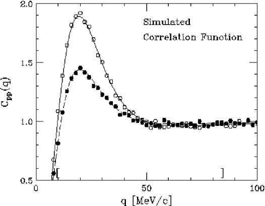
Figure 3: Comparison of original correlation function and restored correlation function. The solid line is the correlation function from the source in Equation (23) and the dashed line is from the source in Equation (24). We obtained the wavefunctions in the kernel in (6) by solving the Schrödinger equation with the REID93 potential [S⁺94]. The symbols represent the correlation functions with added random noise; the noise has a rms magnitude of 0.015. The square brackets above the horizontal axis indicate the range of $q$ we used to restore source.

The results of applying our procedure to the simulated pp correlation function of the preceding section, are shown in Figure 4, for $N=7$. The optimal intervals for discretization typically increase in size with $r$. For example, the first interval in Figure 4 is 2 fm wide and the sixth is 3.6 fm wide. The figure clearly shows that we can satisfactorily restore the source without imposing any constraints. Figure 5 shows the results from a similar restoration of the source with an exponential tail:

$$S(r)={1\over 2}\,{1\over(2\pi R_{0}^{2})^{3/2}}\exp{\left(-\,{r^{2}\over 2R_{0}^{2}}\right)}+{1\over 2}\,{15\over 4\pi^{5}R_{1}^{4}}\,{r\over\exp{(r/R_{1})}-1}\,,$$ (24)

where $R_{0}=3.5$ fm and $R_{1}=6$ fm. We show the correlation function corresponding to the restored source in Figure 3, both with and without errors and random noise with an rms magnitude of 0.015. Since the same $N$ and the same $\{q_{i},\Delta C_{i}\}_{i=1,\ldots,M}$ are used in the inversion, we find the same optimal $\{r_{j}\}_{i=1,\ldots,N}\,$used in Figure 4. The restored source gives evidence for the tail in the source, despite of the fact that the magnitude of the tail is lower by 2 orders of magnitude compared to the maximum at $r=0$. Comparing Figures 4 and 5, we see that our method can discriminate between the two source shapes. If we impose additional constraints to the optimized discretization method, the agreement between the restored and original source functions improves.

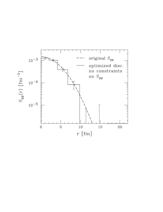
Figure 4: This plot is the same as Figures 6 and 7, except that the source is not constrained and is restored with the Optimized Discretization method.

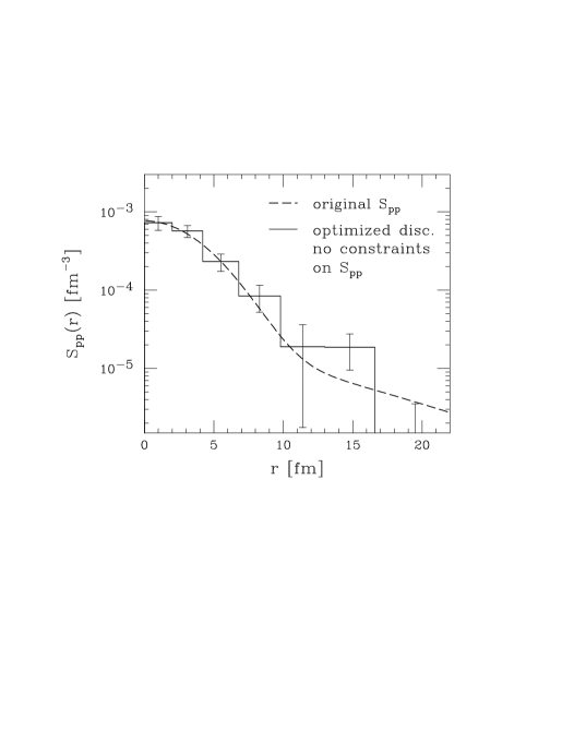
Figure 5: The solid histogram is the relative pp source restored using the Optimized Discretization method. The correlation function used is the solid data in Figure 3. The original source function is shown with the dashed line.

So, while imposing constraints on the source stabilizes the inversion (as we will show in the next subsection), we have developed an imaging method that can yield very satisfactory results even without any constraints. Indeed, one may want to see directly whether the data are consistent with positive definite sources.

5 Constraints

In the Optimized Discretization method, we used the specific behavior of the kernel and the data to improve the inversion. We can also use the source itself, or at least known properties of the source, to stabilize the inversion further. We do this by adding constraints as first suggested by Tikhonov [Tik63]. In practice this amounts to Monte Carlo sampling the error on the experimental data to construct a test correlation function, inverting the test correlation, and testing whether the test source obeys a known set of constraints. If the source is not acceptable, we discard it. We repeat this sampling until we have enough statistics to report the source and its error.

Without using either Optimized Discretization or constraints, it is difficult to obtain stable images. To illustrate how serious an issue of stability is, take the Gaussian source used in Figure 4. Applying the straight algebraic approach yields the results in Figure 6. Clearly the errors for restored source far exceed the original source function. In fact, every second value of the restored source is negative. Incidentally, this is one of our more fortunate simulations, since all of the errors actually fit on the plot.

We next illustrate the dramatic stabilizing effect that the constraints have on the imaging, as it was first discussed by Tikhonov [Tik63]. We carry out the inversion using the same correlation function and errors that we used for Figure 4. We impose the constraints that the imaged source is positive definite, i.e. $S_{j}\geq 0$, as expected in the semi-classical limit, and that the source is normalized: within the restored region $1\geq 4\pi\int_{0}^{r_{N}}dr\,r^{2}\,S\approx 4\pi\sum_{j=1}^{N}S_{j}\int_{r_{j-1}}^{r_{j}}dr\,r^{2}$. Following the general strategies [D’A95] for estimating values with errors under constraints, we carry out our imaging by sampling the values of the correlation of function according to the errors $\{\Delta C_{i}\}_{i=1,\ldots,N}$ (equal to 0.015 in our case) and by applying (18). This amounts to the replacements in (18): $C_{i}\rightarrow C_{i}+\Delta C_{i}\,\xi_{i}$, $i=1,\ldots,N$, with $\xi$’s drawn from the standard normal distribution. We accept only those samplings where the constraints are met. With these samplings, we calculate the average source values and the average dispersions. The results are shown in Figure 7 together with the original source. They now compare favorably to the original source.

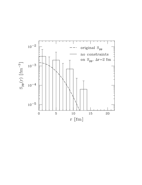
Figure 6: Comparison of the original source with the source restored without constraints. The solid histogram is the source function $S$ restored from the simulated correlation function with the open symbols in Figure 3. The dashed line is the original source function in (23) used to generate the correlation function. We used fixed intervals of $\Delta r=2$ fm for discretizing the source function.

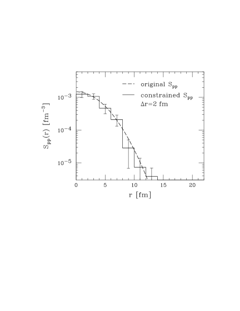
Figure 7: This plot is the same as Figure 6, except that the restored source is constrained to be positive and is normalized to one.

Clearly usage of constraints helps to stabilize the images, so what constraints can be used during imaging? We have already mentioned two: normalization and positivity. One other that we have used takes advantage of the fact that the source for like particle pairs is actually the convolution of the single particle sources in Equation (22). Fourier transforming Equation (22) we find that the Fourier transform of the source must be positive definite:

$$\int{d}^{3}r\>e^{i\vec{r}\cdot\vec{q}}S(\vec{r})=|g(\vec{q})|^{2}\geq 0$$ (25)

where the $g$’s are Fourier transforms of the time-integrated single particle sources (see Equation (2)). For the angle averaged source, this constraint is written in terms of a spherical Bessel function:

$$\int_{0}^{\infty}{d}r\>r^{2}S(r)j_{0}(qr)\geq 0.$$ (26)

Another constraint one might use [Tik63, B⁺80, dH80] is an assumption of smoothness of the source, permitting inversion with more points in the image then there are in the data. Cutting off the integral in the Fourier-transform method [BD97] at $q_{\rm max}$ implies the constraining assumption that $S$ varies slowly on the scale of $1/(2q_{\rm max})\approx 1.2$ fm in [BD97], which is reasonable given the range of strong interactions. Finally we comment that, in imaging terms, the common Gaussian parameterization of sources in heavy-ion collisions is a very extreme constraint for stabilizing the inversion.

3 Generalized Chaoticity Parameter

Just as important as what is in the images, there is a quantity that characterizes what is not in the images. This parameter is the generalized chaoticity parameter and is defined as the integral of the source over a region where the source is significant:

$$\lambda(r_{N})=\int_{r<r_{N}}{d}^{3}r\>\,S(\vec{r})\,.$$ (27)

This symbol, $\lambda(r_{N})$, is a generalization of the the chaoticity $\lambda$ used to parameterize high-energy $\pi\pi$ correlations. The standard chaoticity parameter is defined by fitting the $\pi\pi$ correlation function to a Gaussian:

$$C(q)-1={2\pi\over q}\int_{0}^{\infty}dr\,r\,\sin{\left(2qr\right)}S(r)\simeq\lambda\exp{\left(-\,{4q^{2}R_{0}^{2}}\right)}\,.$$ (28)

When we uses this parameterization of the correlation function, we are assuming this parameterization of the source:

$$S(r)\approx{\lambda\over(2\pi R_{0}^{2})^{3/2}}\exp{\left(-\,{r^{2}\over 4R_{0}^{2}}\right)}.$$ (29)

Our chaoticity parameter generalizes the one in (28) and (29) in two ways. First, the integral defining the generalized chaoticity parameter extends only up to some cut-off, $r_{N}$. The conventional definition of $\lambda$ can be recovered from ours by extending $r_{N}\rightarrow\infty$. Second, because our chaoticity parameter is defined in terms of the imaged source function, rather than a Gaussian fit to the correlation function, it can apply to any particle pair, not just pion pairs.

The importance of our definition of the generalized chaoticity parameter lies in the fact that some particles in the reaction, such as pions or protons, can stem from long-lived resonances and be emitted far from any other particles. Thus, they contribute primarily to $S$ at large $r$, outside the imaged region. For large $r$ and moderate-to-high $q$, the kernel $K$ averages the large-$r$ tails in $S$ to zero so they would not contribute to deviations of $C$ from 1 in Equation (1) or (28). In practice, it should be only possible to directly detect the tails in $S$ by investigating the low-$q$ correlation functions for charged particles. For the analyzed pp data [G⁺90], this $q$-region is either not available or is associated with large systematic errors. Imaging can only extend up to $r_{N}\sim 20$ fm and we expect $\lambda(r_{N})<1$. In many $\pi\pi$ measurements, e.g. [BEC97], the resolution allows one to image regions of comparable sizes, typically 10–20 fm [BD97]. In contrast to the $pp$ and $\pi\pi$ data, the data on IMF, such as [H⁺96], often extend to low values of relative velocity. This permits imaging up to relative separations as large as 50 fm. For a discussion of this, see Section 7.

4 Freeze-Out Density, Average Phase-Space Occupancy and Entropy

The source function and generalized chaoticity parameter both indirectly tell us quite a bit about the reaction dynamics. For example, the source function tells us the relative emission profile, but in the pair frame. It would be an improvement if we had this profile in the system frame. We show how to get this in this section. Of course, we really want is to see the time-evolution of the entire phase-space density. This is not directly accessible from the source, but we can get at the average phase-space density. From this, we can estimate the entropy.

To get at the source function in the system frame we must make some assumptions. For a rapid freeze-out, the single particle source is given by $D(\vec{p},\vec{r},t)\simeq f(\vec{p},\vec{r})\,\delta(t-t_{0})$ where $f$ is the Wigner function of the particles. For weak directional correlations between the total and relative momentum of pairs and between the spatial and momentum variables, the momentum average of $S$ approximates the relative distribution of emission points for any two particles from the reaction, and not just for the particles with close momenta. Under these conditions, the relative distribution for any two particles is

$${\cal S}(\vec{r})={\int{d}^{3}P\>{d}^{3}p\>{d}^{3}R\>f(\vec{P}/2+\vec{p},\vec{R}+\vec{r}/2)\,f(\vec{P}/2-\vec{p},\vec{R}-\vec{r}/2)\over\int{d}^{3}p_{1}\>{d}^{3}r_{1}\>f(\vec{p}_{1},\vec{r}_{1})\,\int{d}^{3}p_{2}\>{d}^{3}r_{2}\>f(\vec{p}_{2},\vec{r}_{2})}\,.$$ (30)

Rewriting and expanding the numerator in (30):

$$f(\vec{P}/2+\vec{p},\vec{R}+\vec{r}/2)\,f(\vec{P}/2-\vec{p},\vec{R}-\vec{r}/2)$$

$$= \int{d}^{3}r_{1}^{\prime}\>\,f(\vec{p}_{1},\vec{r}_{1}^{\prime})\int{d}^{3}r_{2}^{\prime}\>\,f(\vec{p}_{2},\vec{r}_{2}^{\prime}){f(\vec{P}/2+\vec{p},\vec{R}+\vec{r}/2)\,f(\vec{P}/2-\vec{p},\vec{R}-\vec{r}/2)\over\int{d}^{3}r_{1}^{\prime}\>f(\vec{P}/2+\vec{p},\vec{r}_{1}^{\prime})\int{d}^{3}r_{2}^{\prime}\>f(\vec{P}/2-\vec{p},\vec{r}_{2}^{\prime})}$$

$$\begin{split}=&\int{d}^{3}r_{1}^{\prime}\>f(\vec{p}_{1},\vec{r}_{1}^{\prime})\int{d}^{3}r_{2}^{\prime}\>f(\vec{p}_{2},\vec{r}_{2}^{\prime})\left(1+\vec{p}\,{\partial\over\partial\vec{p}^{\prime}}+\ldots\right)\\ &\times\left.{f(\vec{P}/2+\vec{p}^{\prime},\vec{R}+\vec{r}/2)\,f(\vec{P}/2-\vec{p}^{\prime},\vec{R}-\vec{r}/2)\over\int{d}^{3}r_{1}^{\prime}\>f(\vec{P}/2+\vec{p}^{\prime},\vec{r}_{1}^{\prime})\,\int{d}^{3}r_{2}^{\prime}\>f(\vec{P}/2-\vec{p}^{\prime},\vec{r}_{2}^{\prime})}\,\right|_{\vec{p}^{\prime}=0}\,.\end{split}$$ (31)

The gradient term must be proportional to a combination of the vectors $\vec{P}$, $\vec{r}_{1}$, and $\vec{r}_{2}$ and for the weak directional correlations it would average to zero under the integration in (30). Inserting (31) into (30) and keeping the leading term, we obtain

$${\cal S}(\vec{r})\simeq{1\over N^{2}}\int{d}^{3}p_{1}\>\,{d}^{3}p_{2}\>{dN\over{d}^{3}p_{1}\>}\,\,{dN\over{d}^{3}p_{2}\>}\,\gamma_{P}\,S_{\vec{P}}(\vec{r}+\hat{n}_{\vec{P}}\,(\gamma_{P}-1)(\hat{n}_{\vec{P}}\,\vec{r}))\,,$$ (32)

where $N$ is particle multiplicity and $\hat{n}_{\vec{P}}=\vec{P}/|\vec{P}|$. The argument of $S_{\vec{P}}$ has been written in the CM frame of an emitted pair and $\gamma_{P}$ is the Lorentz factor for the transformation from the system frame to the pair CM frame. In general, the relative distribution of emission points for any two particles with $r\rightarrow 0$, when multiplied by $N-1$, gives an average freeze-out density. Thus, if the assumptions above are valid, this density may be obtained by multiplying the average (32) of $S_{\vec{P}}(r\rightarrow 0)$ by $N-1$.

We can estimate the phase-space occupancy at freeze-out regardless of any correlations between momentum of coordinate variables or of the validity of instantaneous freeze-out. The product of the $r\rightarrow 0$ source function and the momentum distribution yields the configuration-space average of the phase-space occupancy at freeze-out,

$$\langle f\rangle(\vec{p})={(2\pi)^{3}\over 2s+1}\,{E_{p}\over m}\,{dN\over{d}^{3}p\>}\,S_{2\vec{p}}(r\rightarrow 0)\,,$$ (33)

as is discussed in [Ber94, Ber96]. Equation (33) can then be used to determine the phase-space average of the occupancy at freeze-out,

$$\langle f\rangle=\int{d}^{3}p\>(\langle f\rangle(\vec{p}))^{2}\,/\int{d}^{3}p\>\,\langle f\rangle(\vec{p}),$$ (34)

and to estimate the entropy per particle,

$${S\over A}\approx-\,{\int{d}^{3}p\>\left(\langle f\rangle(\vec{p})\,\log{\left(\langle f\rangle(\vec{p})\right)}-\left(1-\langle f\rangle(\vec{p})\right)\,\log{\left(1-\langle f\rangle(\vec{p})\right)}\right)\over\int{d}^{3}p\>\langle f\rangle(\vec{p})}\,.$$ (35)

Now, the average phase-space occupancy at freeze-out and the entropy per pion are often calculated for pions because this can be done directly from the correlation function [Ber94, Ber96]. What is new here is that, because we use the source function directly, Equations (33)–(35) apply to any type of particle. In particular, we will calculate the phase-space occupancy and entropy per proton in Section 6.

5 Pions and Kaons

As a specific example of the source extraction, we present the inversion of the angle-averaged $\pi^{-}$ source function determined from the central 10.8 GeV/c Au + Au data of Reference [MEC96] and the angle-averaged $\pi^{-}$ and $K^{+}$ source functions determined from the preliminary central 11.4 GeV/c Au + Au data of Reference [Von98]. The comparison of the data sets will show the lack of variation of the $\pi^{-}$ sources with energy and will show the dramatic difference between the $\pi^{-}$ and $K^{+}$ sources. Before presenting this discussion, we will compare inversions of the [MEC96] data set using the Optimized Discretization method and direct Fourier transformation of Coulomb corrected data, demonstrating the consistency of the inversions.

1 Comparison of Inversion Methods

The data of [MEC96] has been Coulomb corrected for the pair Coulomb force. So in the Pratt-Koonin equation, we may use the kernel for a non-interacting pair, $K(q,r)=\sin{(2qr)}/(2qr)$. Thus, the inversion can be done by performing a Fourier transform. In Figure 8, we show the results from this Fourier transform of the correlation function and from using the Optimized Discretization method. Unlike in [BD97], we do note correct the data for the Coulomb interaction between the pions and the source as in [BBM96].

In the Fourier transformed data, the upper and lower lines represent the error band surrounding the average source. We carried out the Fourier inversion in (8) for Figure 8 up to $q_{\rm max}\simeq 50$ MeV/c giving a resolution in the relative distance of $\Delta r\sim 1/2q_{\rm max}\sim 2.0$ fm. The largest $r$ that we should be able to image follows from $1/2\,\Delta q\approx 20$ fm, where $\Delta q$ is the momentum resolution for the data ($\Delta q=5$ MeV/c in the case of [MEC96]).

For the Optimized Discretization results, we again use the non-interacting pion kernel. Ideally we would have liked to do the inversion using the full Coulomb wavefunctions for the kernel as this would increase the overall accuracy of the plot, however the data was corrected using the “finite size Coulomb correction” and a finite resolution correction which we can not unfold.

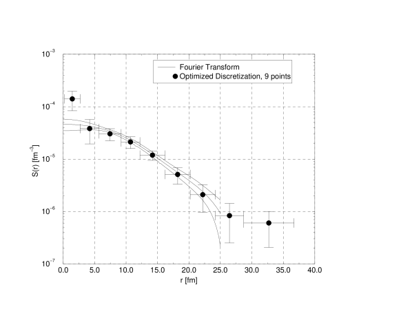
Figure 8: Source function for negatively charged pions from Reference [MEC96].

The results from both inversions are quite consistent except for the lowest r bin in the Optimized Discretization set. This point is at $r=1.45$ fm and at that range, the inter-pion force should receive significant contribution from the nuclear force and neither inversion results should reflect the actual source. In the tail region, where past the edge of the Fourier inverted data, the Optimized Discretization data tends to flatten a bit. This is probably due to the large size of the bins rather than an actual flattening of the source. So, in the end it is comforting to see that the source comes out the same with both methods.

2 Comparison of $\pi^{-}$ and $K^{+}$ Sources

We now discuss the Optimized Discretization results from the $10.8$ GeV/A pion data of [MEC96] and the preliminary $11.4$ GeV/A pion and kaon data sets from [Von98]. The plots of the source functions for these data are shown in Figure 9. The $10.8$ GeV/A $\pi^{-}$ data set was Coulomb corrected and inverted in the manner described above. The $11.4$ GeV/A pion data set was treated differently since it is not Coulomb corrected for the pair Coulomb force. We restored this source using the full Coulomb wavefunctions and the kernel

$$K_{0}(q,r)=\sum_{\ell\,\,{\rm even}}\frac{|g_{\ell}(r)|^{2}}{(2\ell+1)}-1.$$ (36)

The kaon data set was also restored using this kernel and the full Coulomb wavefunctions. In both the pion and kaon cases, the inter-meson nuclear forces were neglected as they are only important at distances $\lesssim 1$ fm for the momenta of interest.

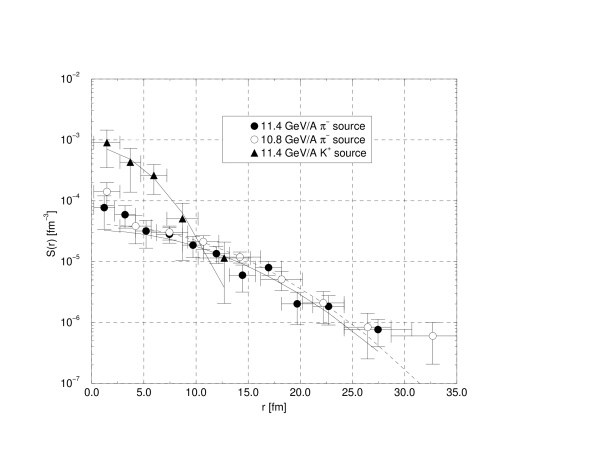
Figure 9: Comparison of the negatively charged pion source functions from the Au + Au reaction at $11.4$ and $10.8$ GeV/A and positively charge kaon source functions from the same reaction at $11.4$ GeV/A.

Examining Figure 9, several things are apparent. First, we note that both $\pi^{-}$ data sets are consistent despite the difference in beam energy and the difference in centrality cuts ($\sigma/\sigma_{\rm geom}<10\%$ for the $10.8$ GeV/A data versus $\sigma/\sigma_{\rm geom}<4\%$ for the $11.4$ GeV/A data). Because the higher energy data set has roughly five times the statistics of the lower energy set, we can restore with higher resolution.

The next thing we notice is that the kaon source is more compact than the pion sources. Because the temporal and spatial evolution of the single particle sources is entangled in the source function in a non-trivial way (see Equation (2)), the difference in sources sizes can be attributed to either life-time effects, emission time effects, real differences in the source size or a combination of the three. First, a sizeable fraction of the pions are the products of resonance decays such as the $\omega$, $\rho$, $\eta$ and $\eta^{\prime}$ (the rest are produced directly) while the majority of the kaons are produced directly or via the decay of $K^{*}$’s. Since both the $\eta$ and $\eta^{\prime}$ decay at distances much greater than $35$ fm (the $\eta$ lifetime is $1.6\times 10^{5}$ fm/c and the $\eta^{\prime}$ lifetime is $980$ fm/c), decays from these resonances do not contribute to the shape of the pion source. Comparing the lifetimes of the $\rho$ ($1.3$ fm/c) and the $\omega$ ($23$ fm/c), it would seem that $\omega$ decay would have the greatest effect on the shape of the pion source, provided they are produced in sufficient numbers. Similarly, the decay of the $K^{*}$ would have a great effect on the kaon source as it’s lifetime ($3.9$ fm/c) is comparable to the size of its source. Second, the difference in the pion and kaon sources may be attributed to emission time effects. Given that the pion mass is roughly $1/3$ the kaon mass, the pions will have a larger average velocity. Comparing a kaon pair and a pion pair, both created with a similar time separation, the early pion can travel much farther the early kaon could – extending the pion source relative to the kaon source. Finally, the pions may be emitted for a larger source region than the kaons. The cross sections for the pions to interact with the particles in the system are, on the average, larger than the kaon cross sections. This means that the pions couple to the system more strongly and so are more effected by the system’s evolution. Since the colliding system expands as it evolves, the source size of the pions could be attributed to the pions being emitted at a later stage in the system’s evolution than the kaons.

Unentangling which combination of effects is responsible for the difference between the $\pi^{-}$ and $K^{+}$ sources could be accomplished either through modeling or further experimentation. We have not yet performed model calculations for this reaction but calculations for similar reactions at CERN energies have been performed by Sullivan and coworkers [S⁺93] and many of their qualitative results are applicable at AGS energies. First, they find that most of the kaons stem from the decay of $K^{*}$’s and string fragmentation. There are few (if any) strings at AGS energies, so it is likely that our kaons stem solely from $K^{*}$ decays. Second, they find that a majority of pions are produced in secondary collisions or via short-lived resonance decays (meaning those with lifetimes $\leq 2$ fm/c). However, they also found that a large fraction of pions are made from long-lived resonance decays (with lifetime $>2$ fm/c). The long-lived resonance contribution dominates at distances of about 10 fm onwards with the longest-lived resonances (the $\eta$ and $\eta^{\prime}$) producing 1 out of every 4 pions in the central rapidities at SPS energies. So, it would seem that a combination of effects can explain why the kaon source is narrower that the pion sources. We could also unravel which combination of scenarios gives the difference in source sizes by using the full three-dimensional correlation function. With the full source function, we would look for elongation in the $\vec{P}$ direction. A difference in emission time of the pair would show up as an elongation in the direction of the average relative velocity of the pair and this average velocity is parallel to the total momentum of the pair.

Let us now move beyond discussion of the size of the pion and kaon sources and examine the integrals of the sources and what we can learn from Gaussian fits to the sources. Now, all three data sets appear Gaussian so we can fit the sources with the Gaussian parameterization

$$S(r)=\frac{\lambda_{\rm fit}}{(2\sqrt{\pi}R_{0})^{3}}\exp{\left(-\left(\frac{r}{2R_{0}}\right)^{2}\right)}$$

Results from the fits are listed in Table 1. In this table, we have also tabulated the integrals of the sources over the entire imaged region. In all three cases, the integrals of the source, a.k.a. the generalized chaoticity parameter, are consistent with the fit parameter $\lambda_{\rm fit}$. The fit parameter $\lambda_{\rm fit}$ is usually identified as the chaoticity parameter. The fact that the integral of the kaon source is consistent with $1$ tells us that the entire source is within the imaged region. The fact that both pion sources are not consistent with $1$ tells us that much of the pion sources must lie outside of the imaged region. In fact, we could estimate that roughly $40\%$ of the pion pairs have one or both pions emitted farther than $35$ fm from the center of the reaction zone. What could account for this long-distance emission? The most obvious answer is resonance production of the pions. The $\omega$ decays with a lifetime of $23$ fm/c so it might account for a tail near the edge of the image – higher resolution correlations (especially near $q\approx 0$) might show evidence for this long-distance decay. The $\eta$ and $\eta^{\prime}$ decays are much longer – the lifetimes are $1.6\times 10^{5}$ fm/c and $980$ fm/c respectively. Pion production from either of these resonances could not be detected directly with our imaging method but could account for $\lambda(35{\rm fm})$ being less than one.

Table 1: Listing of Gaussian fit parameters and the integrals of the source for the pion and kaon sources.

	$R_{0}$ [fm]	$\lambda_{\rm fit}$	$\lambda(35{\rm fm})$
$K^{+}$ (11.4 GeV/A)	2.76	0.702	0.86$\pm$	0.56
$\pi^{-}$ (11.4 GeV/A)	6.42	0.384	0.44$\pm$	0.17
$\pi^{-}$ (10.8 GeV/A)	6.43	0.486	0.59$\pm$	0.22

6 Protons

Now we apply the Optimized Discretization method to analyze the pp correlation data [G⁺90, G⁺91] from the ¹⁴N +²⁷Al reaction at 75 MeV/nucleon, that we imaged in a naive fashion in Reference [BD97]. Since this method does not require a positive definite source to stabilize the image, we are able to lift this constraint and verify whether the data favor positive definite sources. Further, we do not need to normalize the sources to one within the imaged region. We also compare the pp sources from data to those from the transport model [Dan95], over a large range of relative separations and magnitude of the sources. Past experiences in comparing semi-classical transport models to single-particle and correlation data have been mixed [G⁺90, G⁺91, G⁺93, H⁺95, G⁺95], for this particular reaction and others in this energy range.

In Reference [G⁺90, G⁺91], the low relative-momentum pp-correlations were determined for pairs emitted around $\theta_{\rm lab}=25^{\circ}$ from the ¹⁴N + ²⁷Al reaction at 75 MeV/nucleon, in three intervals of the total momentum: 270–390, 450–780, and 840–1230 MeV/c. The highest lab momenta interval corresponds to the highest proton momenta in the participant CM for this reaction. These momenta are higher than the average for participant protons and directed rather forward. Transport calculations [BD97, Dan95] show that the highest momenta bin is mostly populated by pairs from the semi-central to peripheral collisions. The intermediate momenta interval corresponds to the magnitude of typical momenta of participant nucleons in the forward NN CM hemisphere. The transport calculations show that these pairs stem mainly from the semi-central collisions. The lowest lab momenta interval has both participant and target spectator contributions. In the latter case, the transport calculations show that pairs are mostly from the semi-central to central collisions. According to the transport model, the average emission times for protons in the three momenta intervals, from the first contact of the nuclei, are $\sim 35$, $\sim 80$, and $\sim 110$ fm/c, respectively.

The results of analyzing data using the Optimized Discretization method are presented in Figure 10 The angle and spin averaged kernel that we used to produce these images is [BD97]

$$K_{0}(q,r)={1\over 2}\sum_{js\ell\ell^{\prime}}(2j+1)\,\left(g_{js}^{\ell\ell^{\prime}}(r)\right)^{2}-1\,,$$ (37)

where $g_{js}^{\ell\ell^{\prime}}$ is the radial wave function with outgoing asymptotic angular momentum $\ell$. While we only show the source obtained using wavefunctions for the REID93 potential, the values for the NIJM2 [S⁺94] differ only by a fraction of $1/1000^{\rm th}$. Both sources imaged with and without constraints are similar; given their errors we only plot the constrained source in the figure. The results obtained without constraints are generally consistent with positive definite source functions.

In Figure 10, we compare the constrained results from the data to the distributions of relative separation of last collision points for protons with similar momentum from the transport model [BD97, Dan95]. Clearly, the semi-classical model can only yield positive-definite source functions. Again, we can see the focusing of the experimental distribution at low $r$ as the pair momentum increases. The large-$r$ tails in the distribution at different momenta cannot be accommodated with the Gaussian parameterizations used to describe the low-$r$ behavior of the sources [G⁺90, G⁺91].

Generally (see Figure 10), the Boltzmann-equation model (BEM) yields relative emission point distributions that are similar to the imaged data, including the dependence on total pair momentum. In fact, the maximae around $q=20$ MeV/c (such as in Figure 3) are nearly the same height as the data (see Figure 2 in [G⁺93]). Such findings are somewhat surprising for the low and intermediate total momentum intervals. While BEM adequately describes high-momentum wide-angle single-particle spectra of protons, which correspond to the highest total-momentum interval (see Figure 1 in [G⁺93]), the model overestimates the single-particle proton spectra by as much as 1.5–5 in the two lower momentum intervals [G⁺93]. Looking closer at Figure 10, we find that the distributions from data are somewhat sharper at low-$r$ in the two lower total-momentum intervals than the the distributions from the model. In the next section, we reveal a serious discrepancy when we go beyond a point by point examination.

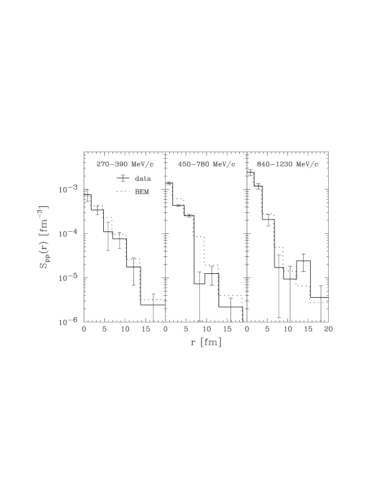
Figure 10: Relative proton source from the ¹⁴N + ²⁷Al reaction at 75 MeV/nucleon, in the vicinity of $\theta_{\rm lab}=25^{\circ}$, in the three total momentum intervals of 270–390 MeV/c (left panel), 450–780 MeV/c (center panel), and 840–1230 MeV/c (right panel). Solid lines are the source values extracted from the data [G⁺91] and the dotted lines are the source values obtained in the Boltzmann-equation calculation.

Table 2: Comparison of the integral of the relative pp source function, $\lambda(r_{N})$, for the restored and BEM sources in three total momentum gates. The restored sources use the data of Reference [G⁺90]. The integrals are truncated at the distance $r_{N}$.

$P$-Range	$\lambda(r_{N})$					$r_{N}$
[MeV/c]	unconstrained		constrained		BEM	[fm]
270-390	0.69$\pm$	0.22	0.69$\pm$	0.15	0.98	20.0
450-780	0.560$\pm$	0.065	0.574$\pm$	0.053	0.91	18.8
840-1230	0.65$\pm$	0.37	0.87$\pm$	0.14	0.88	20.8

1 Integral of Proton Source and Its Implications

In Table 2, we have tabulated $\lambda(r_{N})$ in each momentum interval for the constrained and unconstrained sources as well as sources from the BEM. Comparing the results of the BEM to the constrained source, we only find agreement in the highest momentum interval. It seems that, when compared to the model, significant portions of the source are missing from the imaged regions. This discrepancy is especially pronounced in the intermediate-momentum region. Nevertheless, it is comforting that the transport model describes the features of the relative source for the high momentum protons since it properly describes [G⁺93] the high-momentum single-particle spectra. Now, in BEM no IMFs are produced and the IMFs may decay over an extended time, contributing to large separations in the relative emission function, as they move away from the reaction region. Of course these decays produce some final IMFs, contributing to the relative IMF sources at distances similar to those for the pp sources. It may be interesting to see whether a significant portion of the relative IMF sources in Section 7 can extend beyond $\sim 20$ fm, as is apparent for the pp sources.

The disagreements between the data and calculations in both the values of $\lambda(r_{N})$ and the single-particle spectra [G⁺93], for the lower momenta, reveal unphysical features of low-momentum proton emission in the transport model. The coarse agreement between the measured correlation function and the function calculated using the model in Reference [G⁺93] in the lower total-momentum intervals is coincidental. Since the images show $\lambda(r_{N})<1$, some of the strength of $S$ is shifted out to large $r$ and a large source results in a correlation function with a sharper shape. Thus, the BEM correlation function can match the height of the sharper correlation peak, while not matching the shape of the peak. For other systems in the general energy range, disagreements were found even for the height of $C$ [G⁺91, H⁺95, G⁺95].

These conclusions make us question the sensibility of attempting to fit the magnitude of pp (or nn) correlation functions at the maximum [BGJ90, G⁺90, G⁺91] by adjusting the radius $R_{0}$ while keeping $\lambda=1$ in a Gaussian parametrization of the source function (such as in Equation (29)). When one fits $\pi\pi$ correlation functions at intermediate relative momenta, one varies both the strength and extent of the source function at low $r$: $\lambda$ is read off from the magnitude of the correlation function at low $q$ and $R_{0}$ is read off from the width of the correlation function in $q$. However, because of the resonant nature of the low-momentum NN interaction the magnitude of NN correlation functions are determined by the strength of the source within the resonance peak of the wavefunction. That amount is both effected by the strength of the source at low-$r$ and the low-$r$ source falloff. This is illustrated in Figure 11 which shows pp correlation functions for the source in (29): the same maximum height can be obtained using $R_{0}=4.5$ fm and $\lambda=1$ as using $R_{0}=3.5$ fm and $\lambda=0.5$.

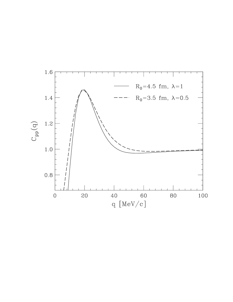
Figure 11: The solid line is the two-proton correlation function for $R_{0}=4.5$ fm and $\lambda=1$ while the dashed line is for $R_{0}=3.5$ fm and $\lambda=0.5$. The source is the Gaussian in Equation (29).

Given that the resonance peak in the ${}^{1}S_{0}$ wavefunction is quite narro (it has an outer radius of $\sim 2.5$ fm), and the source falloff cuts off large-$r$ contributions to the integration in Equation (1), the low-$r$ limit of $S$ is proportional to the $C-1$ at the maximum (to a $\pm 20\%$ level) for virtually all low-$r$ falloffs that may be encountered in practice (namely, $R_{0}=2.5-6.0$ fm):

$$C_{\vec{P}}(20\,{\rm MeV/c})\approx 1+520\,{\rm fm^{3}}\,S_{\vec{P}}(r\rightarrow 0).$$ (38)

For the two sources in Figure 11, we get about the same value of $S(r\rightarrow 0)$ and therefore about the same maximum height in $C$. With the same maximum height, the source falloff is reflected in the width of the maximum in Figure 11.

2 Nucleon Freeze-Out Density, Proton Phase-Space Occupancy and the Entropy per Nucleon

Now that we have discussed the pp data, let us see what we can learn about the final, freeze-out, conditions of the reaction. From the source, we can estimate the nucleon freeze-out density, the average proton phase-space occupancy at freeze-out and entropy per nucleon. First, we need to know which momentum gate best represents the average situation in nearly central collisions. Transport calculations [Dan95] indicate that the measured [G⁺91] coincidence cross sections for the ¹⁴N + ²⁷Al reaction are dominated by nearly central collisions with $b\sim 2.8$ fm. The chance of detecting two particles at a wide angle simultaneously is large only for such collisions. The rms nucleon CM momentum in these collisions is $\sim 185$ MeV/c. At 25^∘ this corresponds to $\sim 320$ MeV/c nucleon laboratory momentum, or $\sim 640$ MeV/c total momentum for a pair. Thus, the results for the intermediate-momentum gate in Figure 10 best represent the average situation in central collisions.

We can estimate the freeze-out nucleon configuration-space density. We start with Equation (32) and use the assumptions of Section 4, together with the presumption that the relative spatial distributions of other particles to protons is similar to that between two protons. We further assume the participants to have a total mass of 18 and to be in a fireball geometry with $b\approx 2.8$ fm. Given this, the proton relative spatial distribution gives the average nuclear density in the vicinity of any emitted proton of $17\times S(r\rightarrow 0)\simeq 17\times 0.0015$ fm${}^{-3}=0.025$ fm${}^{-3}=0.16\,n_{0}$, where $n_{0}$ is the average nuclear density. The directional space-momentum correlations due to collective motion, to shadowing, or to emission that is most likely not instantaneous make this value actually an upper limit on the freeze-out configuration-space density.

We can also estimate the proton phase-space density at freeze-out and, from that, the entropy per nucleon at freeze-out. References [G⁺91, G⁺93] give the inclusive proton cross-sections in the ¹⁴N + ²⁷Al reaction, but only at two angles and the cross sections include large contributions from peripheral events. Under these circumstances, we use the thermal distribution $dN_{\rm th}/{d}^{3}p\>\propto 1/(z^{-1}\,{\rm e}^{p^{2}/2mT}+1)$, for the central events, in formula (33). Here $z$ is set from the requirement of maximum entropy. For $\sim 9$ participant protons at $b=2.8$ fm in the ¹⁴N + ²⁷Al reaction, that requirement gives $z\sim 1.10$ and $T\approx 10.2$ MeV. Use of the thermal momentum distribution for the ¹⁴N + ²⁷Al reaction in Equations (34) and (35) yields $\langle f\rangle\approx 0.23$ and $S/A\approx 2.7$. For a distribution with non-equilibrium features, these values should represent the lower limit on the average occupation and the upper limit on the entropy. Indeed, when applied to the transport model, using a thermal distribution yields an entropy about 0.5 per nucleon higher than the entropy calculated directly within the model.

7 Intermediate Mass Fragments

We now turn to the analysis of IMF sources. We choose the correlation data of Hamilton et al. [H⁺96], from central ⁸⁴Kr + ¹⁹⁷Au reactions at 35, 55, and 70 MeV/nucleon, because these data give us the opportunity to examine the variation of sources with beam energy.

Hamilton et al. collected pairs in the angular range of $25^{\circ}<\theta_{\rm lab}<50^{\circ}$ in order to limit contributions from target-like residues. They tabulate the correlation functions in terms of the reduced velocity

$$v_{\rm red}={v\over(Z_{1}+Z_{2})^{1/2}}\,,$$ (39)

under the assumptions that the pair Coulomb correlation dominates the fragment correlation and that the fragments were approximately symmetric, $Z/A\approx 1/2$. Under these assumptions and the additional assumption that three body effects can be neglected, the kernel is

$$K_{0}(q,r)=\theta(r-r_{c})\,\left(1-r_{c}/r\right)^{1/2}-1\,,$$ (40)

The distance of closest approach in (40) for symmetric fragments is approximately

$$r_{c}={2\,Z_{1}\,Z_{2}\,(A_{1}+A_{2})\,e^{2}\over A_{1}\,A_{2}\,m_{N}\,v^{2}}\approx{e^{2}\over m_{N}\,v_{\rm red}^{2}}\,.$$ (41)

The correlation functions at the three beam energies are shown in Figure 12. We have reduced the normalization of the correlation function at 35 MeV/nucleon by 5%, compared to [H⁺96] to better satisfy the condition that $C\rightarrow 1$ at large $v_{\rm red}$ (this also allows $C\approx 1$ for $v_{\rm red}=(0.05-0.08)c$, a requirement of the authors in [H⁺96]). When we examine Equations (1),(40), (41) and Figure 12, an issue becomes apparent: only the region of the source with $r>r_{c}$ contributes to the correlation function at a given $v_{\rm red}$. As $v_{\rm red}$ increases from 0, the distance of closest approach $r_{c}$ decreases, with more and more inner regions of the source $S$ contributing to $C$. The low-$v_{\rm red}$ correlation functions at the three beam energies in Figure 12 are quite similar, suggesting that the tails of the source functions are similar. Differences occur at higher $v_{\rm red}$, indicating differences in the inner regions of the source.

To image of the IMF sources, we optimize $\{r_{j}\}_{i=1,\ldots,N}\,$as in the pp case, but we add the constraint $r_{1}\geq r_{1}^{\rm min}$. We do this because the Coulomb interaction in (1) does not dominate when the measured fragments are in close contact. The Coulomb correlation alone cannot be relied upon to get information on the most inner portion of the source. The typical touching distance for the fragments measured in [H⁺96] is $r_{t}\sim 5$ fm; we chose a minimum imaging distance $r_{1}^{\rm min}=7.0$ fm which ensures that there is more volume in the lowest bin outside $r_{t}$, than inside $r_{t}$.

The results from our imaging are shown in Figure 13. Given the errors in the figure, the tails of the sources at the three energies are not very different. However, we observe significant variation with energy at short relative distances ($r<12$ fm) with the source undergoing a larger change between 55 and 75 MeV/nucleon, than between 35 and 55 MeV/nucleon.

In Table 3 we tabulate the generalized chaoticity parameter for the IMF sources with $r_{N}=20$ fm and over the whole image. The $\lambda_{\rm TOT}$ for all three energies are all consistent with one, within errors. Since the $\lambda(20{\rm fm})$ are all 20%-30% lower than $\lambda_{\rm TOT}$, we see that a large part of IMF emission occurs at distances that are not imaged with the protons. Nevertheless, the $\lambda(20{\rm fm})$ for the the low- and high-momentum pp sources in section 6 are roughly equal to the IMF $\lambda(20{\rm fm})$ but the the intermediate-momentum pp $\lambda(20{\rm fm})$ is lower. It should be mentioned that no complete quantitative agreement should be expected, even if the data were from the same reaction and pertained to the same particle-velocity range. This is because more protons than IMFs can stem from secondary decays. Besides, the velocity gained by a proton in a typical decay is large compared to the relevant relative velocities in pp correlations, but the velocity gained by an IMF can be quite small on the scale of velocities relevant for the IMF Coulomb correlations. Thus, the IMF correlations may reflect the primary parent sources, which are concentrated around the origin, rather than the final sources.

The tails of the IMF sources extend so far that they must be associated with the time extension of emission. Even so, it is interesting to ask how far into the center of the source must we go to see where the effects due to the spatial extent of the primary source. In [H⁺96], the combinations of single-particle source radii and lifetimes that gave acceptable descriptions of their data have radii varying between 5 and 12 fm. In general, the combination of spatial extent and lifetime effects should give rise to a bone-like shape of the relative source, with the source elongation being due to the emission lifetime. With this, one could try to separate the temporal and spatial effects using a three-dimensional source restoration. In the angle-averaged source, the part dominated by lifetime effects should fall off as an exponential divided by the square of the separation, $r^{2}$, as a function of relative separation $r$. On the other hand, the part of the relative source dominated by spatial effects may fall off at a slower pace or even be constant. In Figure 13, we see that the sources change weakly with $r$ at 35 and 55 MeV/nucleon and faster at 70 MeV/nucleon, within the range where sources vary with energy ($r\lesssim 12$ fm). For reference, in the insert to Figure 13 we show the IMF source multiplied by $r^{2}$. We see an edge at $r\sim 11$ fm at 35 and at 55 MeV/nucleon which disappears at 70 MeV/nucleon. This is consistent with an emission from the spatial region of a radius $R\sim 11/\sqrt{2}\sim 8$ fm that becomes more diffuse, and possibly spreads out, with the increase in energy. The disappearance of the sharply pronounced spatial region at 70 MeV/nucleon agrees with the general expectation on the IMF production in central symmetric collisions or from central sources in asymmetric collisions that the IMF yields maximize towards 100 MeV/nucleon [Lyn98].

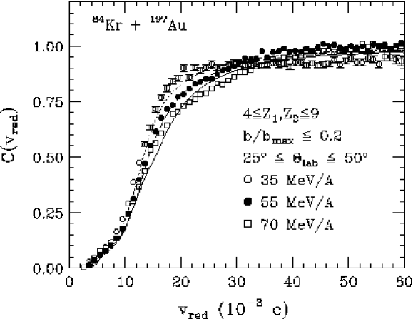
Figure 12: Fragment-fragment velocity correlation function in central ⁸⁴Kr + ¹⁹⁷Au reactions. The symbols show the data of Reference [H⁺96] and the lines show the imaged source function. The 35 MeV/nucleon data is represented by the open circles and dotted line, the 55 MeV/nucleon data by solid circles and dashed line, and 70 MeV/nucleon by open squares and solid line.

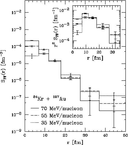
Figure 13: Relative source for IMFs emitted from central ⁸⁴Kr + ¹⁹⁷Au reactions from the data of Reference [H⁺96] at 35 (dotted line), 55 (dashed line), and 70 MeV/nucleon (solid line). The insert shows the source multiplied by $r^{2}$.

Table 3: Comparison of the integrals of the IMF source function, $\lambda(r_{N})$, for different truncation points, $r_{N}$, in three total momentum gates. The restored sources use the data of Reference [H⁺96].

beam energy	$\lambda_{\rm TOT}$		$\lambda(20{\rm fm})$
[MeV/nucleon]
35	0.96$\pm$	0.07	0.72$\pm$	0.04
55	0.97$\pm$	0.06	0.78$\pm$	0.03
70	0.99$\pm$	0.05	0.79$\pm$	0.03

8 Summary

Imaging the source functions from two particle correlation data is possible and we have introduced several methods for doing the inversion. Our most successfull methods use specific features of the kernel or data to aid in the inversion. For example, in the method of Optimized Discretization, we use the behavior of the kernel and the error on the correlation function to adjust the resolution to minimize the relative errors of the source. The fact that we can actually estimate errors in this method gives our method a significant advantage over the Maximum Entropy Method. We tested this method by restoring assumed compact pp sources and found that the quality of the restored source is comparable to the restored source we obtain by imposing the constraints of positivity and normalization. Imposing these constraints in our new method further reduces the source errors, but is no longer required. This method allows one to study the long-range source structure by adjusting the overall size of the imaged region and the resolution at large distances.

The robustness of our imaging method gave us the capability to search for features of the sources that can not be seen in any other analysis. For example, we can look for the resonance contribution to pion sources in [MEC96] or check the positive definiteness of proton Wigner sources in the ¹⁴N + ²⁷Al reaction at 75 MeV/nucleon [G⁺90, G⁺91]. In principle, unraveling the quantal negative values of a Wigner function is not far fetched. In fact, negative values of Wigner functions have been observed in interfering atomic beams [KPM97]. Admittedly, if we had discovered such values in the heavy-ion reactions, we would first have to check for a possible breakdown of the assumptions leading to (1) and on systematic errors in data, before concluding on a success. The extensive averaging in the reactions makes it unlikely that a genuinly quantal oscillation in the source function would survive except in the very tail of the function.

Our analysis of pion and kaon source in Au-Au collisions at $\sim 11$ GeV/A show that the kaons stem from a much smaller source region than the pions. This is likely to be due to a combination of emission time and source size effects. Both the pions and the kaons are produced directly and from the decay of short lived resonances, so their sources should be dominated by the shape of emitting region. However, because the pions are lighter and couple more strongly to the system, they are subject to various dynamic effects that can extend their source function relative to the kaon source function. When examining the generalized chaoticity parameters of the sources, we find the kaons have a $\lambda$ consistant with one, indicating that we have imaged the entire source. We also find that the pion $\lambda$ is not consistant with one, indicating that a large fraction of pions are emitted at large distances ($\gtrsim 35{\rm fm}$). This large distance emission is likely due to contributions from the decay from long-lived resonances such as the $\eta$ and $\eta^{\prime}$.

We found that our imaged proton and IMF sources change significantly with the total pair momentum, becoming sharpest for the largest momenta in the CM. Significant portions of the imaged proton source are missing from the imaged region at typical participant momenta in the CM, but not at the highest momenta. The chaoticity parameter (the integral of the source) from the Boltzmann-equation model [DB91, Dan95] agrees with the data, at the highest momenta but the integral is close to one in the participant and target-emission momenta. Nevertheless, the model yields the correct height of the maximae of the correlation functions [G⁺93]. This is because the right combination of source normalization and sharpness in the model can yield the right value of $S$ at short separations, $S_{\vec{P}}(r\rightarrow 0)$, and this primarily determines the height of $C$. Gaussian-source fits to the height of the pp correlation function [BGJ90, G⁺90, G⁺91] are of a limited value because considerable source strength may lie at large relative separations.

In our analysis of midrapidity IMF sources in central ⁸⁴Kr + ¹⁹⁷Au reactions at different beam energies, we found a significant variation of the sources with energy at short distances, but not at large distances. Considerable portions of the IMF sources extend to large distances ($r>20$ fm) just like the lower total-momentum pp sources. It would be very interesting to image both the IMF and pp sources in one reaction. There is a deficiency of our fragmentation analysis method, namely our method lacks three-body Coulomb effects. When weak, these effects could be included as a first-order perturbation.

While we have made significant progress in the inversion of angle-averaged correlation functions, we have much work to do in the area of inverting full three dimensional data. Unravelling the emission time effects from the three-dimensional sources would be possible because the three-dimensional sources would be distorded in the direction of the pair total momentum. In fact, in the case where lifetime effects dominate the source, we would expect the source to be nearly bone-like in shape [BD97]. In any event, the Optimized Discretization method should prove helpful in inverting three-dimensional data. Finally, the strategy of letting the errors and the kernel choose what source they can image is novel not just for the problem of inverting correlations but the inversion problem in general [P⁺92].

Chapter 4 CONCLUSIONS

Do we fully understand the space-time development of a heavy-ion collision? Definitely not, but the two sets of techniques that we study in this thesis, transport models and nuclear imaging, can play an important role in deducing this space-time evolution at the next generation of nuclear colliders at Brookhaven and CERN. Transport models give us access to the space-time development of collisions by giving the phase-space densities of particles as their output. We studied the application of these models to the massless partons in RHIC collisions. Crucial input to a parton transport model are the initial parton densities. Since it is desirable to be able to connect these phase-space densities to the experimentally determined Parton Distribution Functions, we studied some of the issues associated with constructing a phase-space Parton Model. In contrast to this theoretical effort, nuclear imaging gives us direct access to the space-time development by allowing us to reconstruct the two-particle relative emission distribution from experimental data. Both of these studies are still in their infancy but have yielded many important results.

1 Transport Theory for Partons

Transport models have aided immensely in understanding the space-time evolution of reactions at intermediate energies and we can only hope that they will again aid us as we move into the realm of ultra-relativistic nuclear collisions at RHIC and the LHC. For this to happen, we must have a transport theory applicable to massless partons. We have taken several steps to this goal by providing a scheme that does not rely on either the Quasi-Particle or Quasi-Classical approximations. Instead, the scheme rests upon the phase-space Generalized-Fluctuation Dissipation Theorem which states that the phase-space densities are convolutions of the phase-space source of the particle with the phase-space propagator. We illustrated several ways to calculate the densities in this new framework. These ways include a coupling constant expansion and solving semi-classical transport equations. In both cases, because we have not made either the QCA or QPA we can make controlled approximations based on the strengths of couplings or the size of densities.

In the future, we can hope to advance this approach in several ways. The first job is to understand how renormalization will work in phase-space in particular and non-equilibrium field theory in general. Will we need to dress the vertices and the phase-space propagators or will dressing the densities and letting the masses and couplings run be enough? If we are to renormalize the masses, then we need analytic results for the phase-space propagators for particles with mass. We will also need this propagator if we are to discover if, where and how standard semi-classical transport theory breaks down for lower energy collisions. Also along this track, it would be very useful to understand the interplay and limits of the QCA and QPA in this phase-space approach. Finally, we would like to investigate what it would take to implement bound states in this phase-space approach.

2 Parton Model in Phase-space

A transport model for RHIC or LHC nuclear collisions will need input phase-space parton distributions. We would like to be able to constrain these input distributions using the momentum-space Parton Distribution Functions. Given this, it seems reasonable to wonder if we can rewrite the entire Parton Model in phase-space. As a first step toward this, we examine whether two key tenets of Parton model, namely factorization and evolution, will work in phase-space. We demonstrated the concept of factorization by deriving the QED analog of the parton model, the Weizsäcker-Williams method, in phase-space. We also demonstrated that parton ladder diagrams can be evaluated in phase-space. This is useful because these ladders are the basis of the Leading Logarithm Approximation which is, in turn, equivalent to evolution in the renormalization group improved parton model. The ladder diagram we considered was a simple QED ladder consisting of a point charge radiating a photon which subsequently splits into an on-shell final-state positron and virtual electron. Despite its simplicity, it contains many of the features that we expect from a full-blown QCD parton ladder such as both $1/x_{F}$ and $1/Q^{2}$ type singularities. Furthermore, investigation of this simple ladder shows us how a realistic source distribution shapes the particle phase-space densities. Armed with this understanding, we investigated the size and shape of the parton cloud of a nucleon. We found that the sea parton distributions are roughly the same size as the valence quark bag in the transverse direction and ranged from marginally larger to vastly larger than the valence quark bag in the longitudinal direction.

In the future, we will need quantitative calculations of the parton phase-space densities for input into a transport model. This means a couple of things: this S-matrix based approach must be connected with the time-ordered non-equilibrium approach and we must implement renormalization in the time-ordered non-equilibrium approach. Some of this work has already been done by Makhlin and Surdutovich [Mak95a, Mak95b, Mak96, MS98] however it must be reworked in phase-space.

3 Nuclear Imaging

Directly accessing the space-time development of nuclear reactions through intensity interferometry and nuclear imaging is possible. Results from this approach go far beyond standard Gaussian fits by reconstructing the entire two-particle source functions. We found several methods to perform nuclear imaging and the best ways rely on specific features of the source, the kernel, or the data itself. In fact, the method of Optimized Discretization uses the behavior of the kernel and the error on the correlation function data to choose the best resolution for the source. This method is further improved by using the constraints that the source is known to obey. We applied the inversion methods to several data sets including $K^{+}K^{+}$, $\pi^{-}\pi^{-}$, pp and IMF correlations. An important quantity derived from these sources is the generalized chaoticity parameter which can be used to characterize the amount of the source that lies within, or outside of, the imaged region. The source functions provides other information, namely the freeze-out density and the entropy per nucleon. In total the images provide a great deal more information than previous Gaussian fits and related approaches.

We would like to extend our imaging to invert three-dimensional correlation pion and proton data sets. Such results would be immensely useful in separating the temporal and directional dependence of the sources. Of course there is still much to do for the angle-averaged inversions. We are in the process of analyzing other pion and proton data sets at different energies and with higher resolution. Furthermore, we are developing a set of computer programs that we hope will become generally available for nuclear imaging.

4 Final Remarks

The nuclear physics community has made great strides in understanding the space-time development of nuclear collisions. Nevertheless, our understanding will be tested when we begin to see results from RHIC and the LHC. Is there a quark-gluon plasma? How will it evolve? Our studies of parton transport theory and nuclear imaging should help answer these and many more questions.

APPENDICES

Chapter 5 PHASE-SPACE PROPAGATORS

Quantum particles do not propagate between two space-time points by traveling along straight line classical trajectories. Instead, a particle with fixed 4-momentum can propagate from a point to anywhere in some space-time region defined by its 4-momentum. The propagation is controlled by the phase-space propagators and, in this appendix, we study the retarded and Feynman phase-space propagators in a detail not possible in the main text. Here, we state our phase-space propagators for scalar particles, discuss the symmetries of these propagators, detail both how the retarded and Feynman propagators work, give the derivation of their analytic expressions and, finally, discuss what is needed to treat particles with nonzero mass. The Feynman propagator for particles with nonzero mass has already been discussed by Remler [Rem90] so our discussion here is brief. The Dirac and vector propagators differ from the scalar propagators by the addition of spin projectors so we do not need to discuss them separately.

We define a phase-space propagator as the Wigner transform of two translationally invariant propagators (such as in Equation (34) of Chapter 1 or Equation (6) of Chapter 2):

$${G}\!\left(x,p\right)= \displaystyle\int\frac{{d}^{4}p^{\prime}}{{(2\pi)}^{4}}\>e^{-ix\cdot p^{\prime}}G(p+p^{\prime}/2)G^{\dagger}(p-p^{\prime}/2)$$ (1a)

$$= \displaystyle\int{d}^{4}x^{\prime}\>e^{ix^{\prime}\cdot p}G(x+x^{\prime}/2)G^{\dagger}(x-x^{\prime}/2)$$ (1b)

The vacuum propagators in momentum space are [BS79]:

$$G^{\pm}(p)= -\left(p^{2}-m^{2}\pm i\epsilon p_{0}\right)^{-1}$$ (2a)

$$G^{\stackrel{{\scriptstyle c}}{{a}}}(p)= -\left(p^{2}-m^{2}\pm i\epsilon\right)^{-1}$$ (2b)

In configuration space, the propagators are [BS79]:

$$G^{\pm}(p)= \frac{1}{2\pi}\theta{(\pm x_{0})}\delta\!\left(x^{2}\right)$$ (3a)

$$G^{\stackrel{{\scriptstyle c}}{{a}}}(p)= \frac{1}{4\pi}\left(\delta\!\left(x^{2}\right)\mp{\cal P}\frac{i}{\pi x^{2}}\right)$$ (3b)

As one can see from the configuration space listing, the time ordering is explicit in the retarded propagator while there is no time ordering in the Feynman propagators. This feature is preserved in the phase-space propagators even after the Wigner transforms in (1a)–(1b).

Appendix 5.A The Propagators for Zero Mass Scalar Particles

We now present the Feynman and retarded propagators for particles with zero mass. The advanced and anti-Feynman propagators can be recovered using the symmetry relations discussed in the next section. The propagators are:

$$\begin{split}{G}^{\rm c}\!\left(x,p\right)=&\frac{1}{4\pi}\left[\mbox{ sgn}(x^{2})+\mbox{ sgn}(p^{2})+2\mbox{ sgn}(x\cdot p)\right]\\ &\times\displaystyle\left\{\theta(\lambda^{2})\frac{\sin{(2\sqrt{\lambda^{2}})}}{\sqrt{\lambda^{2}}}-\theta(-\lambda^{2})\frac{\exp{(-2\sqrt{-\lambda^{2}})}}{\sqrt{-\lambda^{2}}}\right\}\end{split}$$ (4a)

$${G}^{+}\!\left(x,p\right)= \frac{1}{\pi}\theta(x_{0})\theta(x^{2})\theta(\lambda^{2})\frac{\sin{(2\sqrt{\lambda^{2}})}}{\sqrt{\lambda^{2}}}$$ (4b)

Here the Lorentz invariant $\lambda^{2}$ is given by $\lambda^{2}=(x\cdot p)^{2}-x^{2}p^{2}$. The retarded phase-space propagator is used throughout Chapters 1 and 2 while the Feynman phase-space propagator is mentioned only in Chapter 2. We discuss how the propagators work in the Sections 1 and 1 and derive the analytic form of each of the propagators in the Sections 2 and 2.

Appendix 5.B Symmetries of the Propagators

Here we list how the phase-space propagators behave under several coordinate transforms. Some of these relations are quite useful because they relate several of the propagators together through simple coordinate reflections.

A time reversal transform in coordinate space is equivalent to a simultaneous reflection in time and energy in phase-space. Under time reversal the $+$ and $-$ propagators change into one another while the Feynman and anti-Feynman propagators remain unchanged:

$${G}^{+}\!\left(x_{0},\vec{x},p_{0},\vec{p}\right)= {G}^{-}\!\left(-x_{0},\vec{x},-p_{0},\vec{p}\right)$$ (5a)

$$G^{\stackrel{{\scriptstyle a}}{{c}}}(x_{0},\vec{x},p_{0},\vec{p})= G^{\stackrel{{\scriptstyle a}}{{c}}}(-x_{0},\vec{x},-p_{0},\vec{p}).$$ (5b)

A parity transform in coordinate space is equivalent to a simultaneous reflection in a space coordinate and the corresponding momentum coordinate. Under a parity transformation, all of the propagators remain unchanged:

$$G^{\pm}(x_{0},\vec{x},p_{0},\vec{p})= G^{\pm}(x_{0},-\vec{x},p_{0},-\vec{p})$$ (7)

$$G^{\stackrel{{\scriptstyle a}}{{c}}}(x_{0},\vec{x},p_{0},\vec{p})= G^{\stackrel{{\scriptstyle a}}{{c}}}(x_{0},-\vec{x},p_{0},-\vec{p}).$$ (8)

The Feynman propagators have another (rather amusing) argument switching symmetry. Here all the space-time components are switched with the the corresponding momentum-energy components:

$$G^{\stackrel{{\scriptstyle a}}{{c}}}(x,p)=G^{\stackrel{{\scriptstyle a}}{{c}}}(p,x)$$ (9)

Finally, the Feynman and anti-Feynman propagator are related through a complete reflection of all of the space or momentum coordinates:

$${G}^{\rm c}\!\left(x,p\right)= {G}^{\rm a}\!\left(-x,p\right)$$ (10a)

$${G}^{\rm c}\!\left(x,p\right)= {G}^{\rm a}\!\left(x,-p\right).$$ (10b)

Appendix 5.C Detail: the Retarded Propagator

The phase-space retarded propagator naturally arose in our discussion of the phase-space Generalized Fluctuation-Dissipation theorem in Chapter 1 and in the discussion of time-ordered amplitudes in Chapter 2. In this section we will describe how the scalar propagator works and how we derive the analytic expression for it at lowest order. A simplified version of the discussion of how the propagator functions is contained in Section 4.

1 How it Works

The Wigner transform of the retarded propagator gives the weight for a particle with four-momentum $q_{\mu}$ to propagate across the space-time separation $\Delta x_{\mu}=x_{\mu}-y_{\mu}$. Without loss of generality, let us give the particle a the momentum $q_{\mu}=(q_{0},q_{L},\vec{0})$ and estimate how far the retarded propagator can send the particle. First, the retarded propagator has two theta functions, one that enforces causality and one that forces propagation inside the light cone. The rest of the interesting features of the propagator are tied up in the dependence on $\lambda^{2}$. Since ${G}^{+}\!\left(\Delta x,q\right)\propto\theta(\lambda^{2})\sin{(\sqrt{\lambda^{2}})}/{\sqrt{\lambda^{2}}}$, the particle does not propagate much farther than the inequalities $0\leq\sqrt{\lambda^{2}}\lesssim 1$ allow. To see what these constraints mean, we investigate the $q^{2}>0$, $q^{2}<0$, and $q^{2}=0$ cases separately.

To study the $q^{2}>0$ case, we position ourselves in the frame where $q^{\prime}_{\mu}=(q^{\prime}_{0},\vec{0})$. In this frame, the $\lambda^{2}$ constraint translates into a restriction on the spatial distance a particle can propagate:

$$0\leq{q^{\prime}_{0}}^{2}|\Delta\vec{x}^{\prime}|^{2}\lesssim 1.$$

Combined with the light-cone constraint, $\Delta\vec{x}^{\prime}$ is constrained to

$$|\Delta\vec{x}^{\prime}|\lesssim\left\{\begin{array}[]{cl}\Delta x^{\prime}_{0}&\mbox{for small}\;\Delta x^{\prime}_{0}<1/|q^{\prime}_{0}|\\ 1/|q^{\prime}_{0}|&\mbox{for large}\;\Delta x^{\prime}_{0}>1/|q^{\prime}_{0}|.\end{array}\right.$$ (11)

To find a cutoff for $\Delta x^{\prime}_{0}$, we realize that, for a given $q^{\prime}_{\mu}$, the propagator gives the “probability” distribution for propagating across the space-time displacement $\Delta x^{\prime}_{\mu}$. Thus, we can integrate ${G}^{+}\!\left(\Delta x^{\prime},q^{\prime}\right)$ over all space and over time up to some cutoff time $\tau$, giving us the total “probability” for propagating to time $\tau$. We find that the propagation probability becomes unimportant for $\tau\gtrsim 1/|q^{\prime}_{0}|$ and this sets a cutoff in $\Delta x^{\prime}_{0}$:

$$\Delta x^{\prime}_{0}\lesssim 1/|q^{\prime}_{0}|.$$ (12)

Together, these three constraints define the space-time region where the particle can propagate. When we move back to the frame with $q_{\mu}=(q_{0},q_{L},\vec{0}_{T})$, the region contracts in the temporal and longitudinal directions. From Equation (12), the limits of the propagation region are

$$|\Delta\vec{x}_{T}|\lesssim R_{\perp}=\frac{1}{\sqrt{|q^{2}|}}$$ (13a)

$$|\Delta x_{L}|\lesssim R_{\|}=\displaystyle\frac{1}{|q_{L}|}$$ (13b)

$$|\Delta x_{0}|\lesssim R_{0}=\displaystyle\frac{1}{|q_{0}|}$$ (13c)

We study the $q^{2}<0$ case in a similar manner. In the frame with $q^{\prime}_{\mu}=(0,q^{\prime}_{L},\vec{0}_{T})$, the $\lambda^{2}$ constraint implies

$$0\leq{q^{\prime}}_{L}^{2}(\Delta{x^{\prime}}_{0}^{2}-\Delta{x^{\prime}}_{T}^{2})\lesssim 1.$$

Combining this with the light-cone constraint immediately gives us a limit on $\Delta x^{\prime}_{L}$:

$$|\Delta x^{\prime}_{L}|\lesssim\frac{1}{|q^{\prime}_{L}|}.$$ (14a)

As with the $q^{2}>0$ case, we can integrate the propagator to find the total “probability” for propagating to the time $\tau$. In this case, the propagation probability is important only for $\tau\lesssim 1/|q^{\prime}_{L}|$, giving us a limit in $\Delta x^{\prime}_{0}$ of:

$$|\Delta x^{\prime}_{0}|\lesssim\frac{1}{|q^{\prime}_{L}|}.$$ (14b)

The limit on $|\Delta\vec{x}^{\prime}_{T}|$ then follows directly from the light-cone constraint:

$$|\Delta\vec{x}^{\prime}_{T}|\lesssim\frac{1}{|q^{\prime}_{L}|}.$$ (14c)

Again, these constraints define a the space-time region where the particle can propagate. Boosting back to the frame with $q_{\mu}=(q_{0},q_{L},\vec{0}_{T})$, again the longitudinal and temporal spread gets Lorentz contracted:

$$|\Delta\vec{x}_{T}|\lesssim R_{\perp}=\displaystyle\frac{1}{\sqrt{|q^{2}|}}$$ (15a)

$$|\Delta x_{L}|\lesssim R_{\|}=\displaystyle\frac{1}{|q_{0}|}$$ (15b)

$$|\Delta x_{0}|\lesssim R_{0}=\displaystyle\frac{1}{|q_{L}|}.$$ (15c)

Now we study the $q^{2}=0$ case. With $q^{2}=0$, $\lambda^{2}$ becomes

$$\lambda^{2}=|\Delta x\cdot q|=|q_{0}||\Delta\vec{x}\cdot\hat{q}-\Delta x_{0}|\lesssim 1.$$ (16)

On other words, high energy particles tend to follow their classical path while low energy particles can deviate from their classical path. Expression (16) then gives a measure of the deviation from the classical path.

2 Derivation

The Wigner transform of $G^{+}$ is easiest to do in coordinate space. In coordinate space, $G^{+}(x)=\frac{1}{2\pi}\theta(x_{0})\delta(x^{2})$, so the Wigner transform integral in Equation (1b) is a series of delta function integrals. Performing the first delta function integral and simplifying the theta functions, we find

$${G}^{+}\!\left(x,p\right)=\frac{\theta(x_{0})}{(2\pi)^{2}}\int^{2x_{0}}_{-2x_{0}}dx^{\prime}_{0}\sqrt{4x^{2}+{x^{\prime}_{0}}^{2}}\int_{4\pi}d\Omega_{\vec{x}^{\prime}}e^{ix^{\prime}\cdot p}\delta(x^{\prime}\cdot x).$$

Using $2\pi\delta(x)=\int^{\infty}_{-\infty}d\alpha e^{ix\alpha}$, we can do the angular integral, giving us a Bessel function:

$${G}^{+}\!\left(x,p\right)=4\pi\theta(x_{0})\theta(x^{2})\int_{-1}^{1}d\alpha e^{i\alpha\eta}J_{0}(\xi\sqrt{1-\alpha^{2}}).$$

Here $\eta=2(p_{0}|\vec{x}|-x_{0}\hat{x}\cdot\vec{p})$ and $\xi=2\sqrt{x^{2}(\vec{p}^{2}-(\vec{p}\cdot\hat{x})^{2})}$. This integral is in any standard integral table [GR94]. After a bit of simplification, one gets the result (4b). This result can be checked by performing the Wigner transforms in momentum space, but the contour integrals needed for this calculation are quite tedious.

Appendix 5.D Detail: the Feynman Propagator

The phase-space Feynman propagator naturally arose in our discussion of the exclusive reaction probabilities in Chapter 2. There we choose situations where we can avoid using the phase-space Feynman propagator. Here we should discuss it anyway. In this section we will describe how the scalar propagator works and how we derive the analytic expression for it at lowest order.

1 How it Works

While the Feynman propagator propagates a particle with a given momentum (say $p_{\mu}=(p_{0},p_{L},\vec{0}_{T})$) across a space-time displacement $\Delta x_{\mu}=(\Delta x_{0},\Delta x_{L},\Delta\vec{x}_{T})$, it does so in a manner very different from the retarded propagator. Looking at the definition in (4a), we see that the combination of the sign functions in the square brackets can be rewritten in a more transparent form:

$$[\ldots]=\left\{\begin{array}[]{ll}4&\mbox{ if }\Delta x\cdot p,\>p^{2},\>\Delta x^{2}>0\\ -4&\mbox{ if }\Delta x\cdot p,\>p^{2},\>\Delta x^{2}<0\\ 2\>{\rm sgn}(\Delta x\cdot p)&\mbox{ if }p^{2},\>x^{2}\mbox{ have opposite sign}\end{array}\right.$$

Thus, particles with time-like momentum tend to travel forward in time and inside the light-cone and particles with space-like momentum tend to travel backwards in time outside the light cone. Anti-particles with time-like momentum tend to travel backwards in time inside the light-cone and anti-particles with space-like momentum tend to travel forwards in time outside the light-cone.

The rest of the interesting features of the Feynman propagator are tied up in the dependence on the Lorentz invariant $\lambda^{2}=(\Delta x\cdot p)^{2}-\Delta x^{2}p^{2}$. As with the retarded propagator in Subsection 4, we will study the $p^{2}>0$, $p^{2}<0$, and $p^{2}=0$ cases separately.

To study the $p^{2}>0$ case, we boost to the frame where $p^{\prime}_{\mu}=(p^{\prime}_{0},\vec{0})$. In this frame, $\lambda^{2}={p^{\prime}}^{2}_{0}|\Delta\vec{x}^{\prime}|^{2}\geq 0$, so only the sine term contributes. The sine term is greatest for $\sqrt{\lambda^{2}}\lesssim 1$ so we have the following limit on the spatial propagation distance:

$$|\Delta\vec{x}^{\prime}|\lesssim\frac{1}{|p^{\prime}_{0}|}.$$ (17a)

As with the retarded propagator, we can compute the total “probability” to propagate to certain time. This calculation gives us the following limit on the temporal propagation distance:

$$|\Delta x^{\prime}_{0}|\lesssim\frac{1}{|p^{\prime}_{0}|}.$$ (17b)

Boosting the space-time region defined by these constraints back to the frame with $p_{\mu}=(p_{0},p_{L},\vec{0}_{T})$, we find the following constraints:

$$|\Delta\vec{x}_{T}|\lesssim R_{\perp}=\frac{1}{\sqrt{|p^{2}|}}$$ (18a)

$$|\Delta x_{L}|\lesssim R_{\|}=\displaystyle\frac{1}{|p_{L}|}$$ (18b)

$$|\Delta x_{0}|\lesssim R_{0}=\displaystyle\frac{1}{|p_{0}|}$$ (18c)

These limits are exactly the same as the ones we found for the retarded propagator in Subsection 4.

To study the $p<0$ case, we boost to the $p^{\prime}_{\mu}=(0,p^{\prime}_{L},\vec{0}_{T})$ frame. In this frame, $\lambda^{2}={p^{\prime}}_{L}^{2}(\Delta{x^{\prime}}_{0}^{2}-\Delta{x^{\prime}}_{T}^{2})$. Inside the light-cone, the exponential term disappears and we get a constraint on $\lambda^{2}$:

$$0\geq\lambda^{2}={p^{\prime}}_{L}^{2}(\Delta{x^{\prime}}_{0}^{2}-\Delta{x^{\prime}}_{T}^{2})\lesssim 1.$$

We can integrate to find the total “probability” to propagate to a certain time, giving us a limit on $\Delta x^{\prime}_{0}$:

$$|\Delta x^{\prime}_{0}|\lesssim\frac{1}{|p^{\prime}_{L}|}.$$ (19)

Using the $\lambda^{2}$ and light-cone constraints, we find similar limits on $\Delta\vec{x}^{\prime}_{T}$ and $\Delta x^{\prime}_{L}$:

$$|\Delta x^{\prime}_{L}|\lesssim \displaystyle\frac{1}{|p^{\prime}_{L}|}$$ (20a)

$$|\Delta\vec{x}^{\prime}_{T}|\lesssim \displaystyle\frac{1}{|p^{\prime}_{L}|}.$$ (20b)

Boosting back to the $p_{\mu}=(p_{0},p_{L},\vec{0}_{T})$ frame, we find

$$|\Delta\vec{x}_{T}|\lesssim R_{\perp}=\frac{1}{\sqrt{|p^{2}|}}$$ (21a)

$$|\Delta x_{L}|\lesssim R_{\|}=\displaystyle\frac{1}{|p_{0}|}$$ (21b)

$$|\Delta x_{0}|\lesssim R_{0}=\displaystyle\frac{1}{|p_{L}|},$$ (21c)

which is what we found for the retarded propagator. Now, outside of the light-cone the situation is more complicated and we must integrate the propagator in the various directions to find limits. We find:

$$|\Delta x^{\prime}_{0}|\lesssim \displaystyle\frac{1}{|p^{\prime}_{L}|}$$ (22a)

$$|\Delta x^{\prime}_{L}|\lesssim \displaystyle\frac{1}{|p^{\prime}_{L}|}$$ (22b)

$$|\Delta\vec{x}^{\prime}_{T}|\lesssim \displaystyle\frac{1}{|p^{\prime}_{L}|}.$$ (22c)

When we boost back to the frame with $p_{\mu}=(p_{0},p_{l},\vec{0}_{T})$, we find the result in Equations (21a)-(21c).

Finally, we investigate the $p^{2}=0$ case. With $p^{2}=0$, $\lambda^{2}$ becomes

$$0\leq\lambda^{2}=|\Delta x\cdot p|=|p_{0}||\Delta\vec{x}\cdot\hat{p}-\Delta x_{0}|\lesssim 1$$ (23)

because the exponential term does not contribute on the light cone. On other words the Feynman propagator functions exactly like the retarded propagator: high energy particles tend to follow their classical path while low energy particles can deviate from their classical path. Expression (23) then gives a measure of the deviation from the classical path.

We find that, despite the different boundary conditions on the two propagators, both the Feynman and retarded propagators send particles the same distances. This is probably no surprise since a calculation done using Feynman’s formulation of perturbation theory for the S-matrix must give the same results as a calculation done using time-ordered non-equilibrium perturbation theory.

2 Derivation

The simplest derivation of ${G}^{\rm c}\!\left(x,p\right)$ is far more complicated than the derivation of ${G}^{+}\!\left(x,p\right)$. We start by finding the transport-like equation of motion for the Wigner propagator. The derivation is simple and very similar to the derivation for the retarded equation of motion in Section 8. So we only state the result:

$$p\cdot\partial\>{G}^{\rm c}\!\left(x,p\right)=\frac{1}{\pi^{2}}\left[\pi\delta(x^{2})\sin{(2x\cdot p)}-{\cal P}\frac{1}{x^{2}}\cos{(2x\cdot p)}\right].$$

Now we define a projector onto the space perpendicular to the particle’s momentum, $g_{\perp\mu\nu}=g_{\mu\nu}-p_{\mu}p_{\nu}/p^{2}$. This allows us to change variables to $x_{\perp\mu}=g_{\perp\mu\nu}x^{\nu}$ and $\tau=x\cdot p/\sqrt{|p^{2}|}\mbox{ sgn}({p^{2}})$. In terms of these variables, we find $\lambda^{2}=-p^{2}x_{\perp}^{2}$ and the equation of motion becomes

$$\partial_{\tau}G^{c}(\tau,x_{\perp},p)=\frac{\mbox{ sgn}(p^{2})\sqrt{|p^{2}|}}{\pi^{2}}\left[\pi\delta(|k^{2}|\tau^{2}-\lambda^{2})\sin{(2\sqrt{|k^{2}|}\tau)}-{\cal P}\frac{\cos{(2\sqrt{|k^{2}|}\tau)}}{|k^{2}|\tau^{2}-\lambda^{2}}\right].$$

So, instead of doing the Wigner transform directly, we only have to solve this ordinary differential equation.

We find the solution by integrating this differential equation. The delta function integral is simple and the principle value integral can be done by contour integration. We find

$$\begin{split}G^{c}(\tau,x_{\perp},p)=&G^{c}(\infty,x_{\perp},p)\\ &-\displaystyle\frac{1}{\pi}\left\{\theta(\lambda^{2})\frac{\sin{(2\sqrt{\lambda^{2}})}}{\sqrt{\lambda^{2}}}\left[\frac{1}{2}(\theta(p^{2})-\theta(x^{2}))+\mbox{ sgn}(p^{2})\theta(-\tau)\right]\right.\\ &\displaystyle\left.-\mbox{ sgn}(p^{2})\theta(-\tau)\frac{\exp{(-2\sqrt{-\lambda^{2}})}}{\sqrt{-\lambda^{2}}}\right\}.\end{split}$$

We must now divine the boundary condition at $\tau\rightarrow\infty$.

To find the boundary condition, we actually have to go back to the Wigner transform of the propagator starting from momentum-space version of equation (1a). We again change variable from $x$ to $\tau$ and $x_{\perp}$. We also change from $p^{\prime}$ to $p^{\prime}_{\perp}=g_{\perp\mu\nu}{p^{\prime}}^{\nu}$ and $p\cdot p^{\prime}=\mbox{ sgn}(p^{2})\sqrt{|p^{2}|}k$. With this, we perform the $k$ contour integral. The integral is straight forward, but tedious. However, when we take the limit as $\tau\rightarrow\infty$, the result simplifies dramatically:

$$G^{c}(\infty,x_{\perp},p)=\frac{1}{\pi^{2}\sqrt{|p^{2}|}}\int{d}^{3}p_{\perp}\>\cos{(2x_{\perp}\cdot p_{\perp})}\delta(p^{2}+p_{\perp}^{2}).$$

The delta function integral is trivial and the last pair of integrals requires integral tables, but in the end we find:

$$G^{c}(\infty,x_{\perp},p)=\frac{1}{\pi}\left\{\theta(\lambda^{2})\mbox{ sgn}(p^{2})\frac{\sin{(2\sqrt{\lambda^{2}})}}{\sqrt{\lambda^{2}}}+\theta(-\lambda^{2})\theta(-p^{2})\frac{\exp{(-2\sqrt{-\lambda^{2}})}}{\sqrt{-\lambda^{2}}}\right\}.$$

Plugging this into the solution of our differential equation, we find Equation (4a). This result can be checked by performing a series of contour integrals in momentum or coordinate space.

Appendix 5.E Propagating Particles with Nonzero Mass

The issue of propagating particles with nonzero is an important one if one is either to dress the particles with an in-medium mass or to test conventional transport theory as applied to nucleons. In this section, we will discuss the beginnings of work aimed at getting analytic expressions for the propagators for particles with nonzero mass. There are two ways that we know for getting the propagator for particles with nonzero mass. The first is a transform we that adds mass to the massless propagators. We demonstrate it on the retarded propagator. The second is an approximation developed by Remler [Rem90] which we will outline and state the results he obtained for the Feynman propagator.

1 The Retarded Propagator

According to (1a), a phase-space propagator is the Wigner transform of two propagators. To find the propagator for particles with nonzero mass, we begin by writing out the Wigner transform of the two retarded propagators in the coordinates where the transfered momentum is $p_{\mu}=(p_{0},p_{L},\vec{0}_{T})$:

$$\begin{split}G^{+}(x,p)=&\int\frac{{d}^{4}p^{\prime}}{{(2\pi)}^{4}}\>e^{-x\cdot p^{\prime}}G^{+}(p+p^{\prime}/2)G^{-}(p-p^{\prime}/2)\\ =&\int^{\infty}_{-\infty}\frac{d{p^{\prime}_{0}}}{2\pi}\int^{\infty}_{-\infty}\frac{d{p^{\prime}_{L}}}{2\pi}\int^{\infty}_{0}\frac{d{{p^{\prime}_{T}}}^{2}}{2(2\pi)^{2}}\int^{2\pi}_{0}\frac{d\theta^{\prime}}{2\pi}e^{-i(x_{0}{p^{\prime}_{0}}-x_{L}{p^{\prime}_{L}}-x_{T}{p^{\prime}_{T}}\cos\theta^{\prime})}\\ &\times\left((p_{0}+{p^{\prime}_{0}}/2)^{2}-(p_{L}+{p^{\prime}_{L}}/2)^{2}-({\vec{p^{\prime}}_{T}}/4+m^{2})+i\varepsilon(p_{0}+{p^{\prime}_{0}}/2)\right)^{-1}\\ &\times\left((p_{0}-{p^{\prime}_{0}}/2)^{2}-(p_{L}-{p^{\prime}_{L}}/2)^{2}-({\vec{p^{\prime}}_{T}}/4+m^{2})+i\varepsilon(p_{0}-{p^{\prime}_{0}}/2)\right)^{-1}\end{split}$$ (24)

Now, we notice that the denominator is independent of $\theta^{\prime}$, so we can perform the $\theta^{\prime}$ integral using the relation

$$\int_{0}^{2\pi}d\theta^{\prime}\>e^{ix_{T}p^{\prime}_{T}\cos{\theta^{\prime}}}=2\pi J_{0}\!\left(x_{T}p^{\prime}_{T}\right).$$

This turns Equation (24) into a Fourier-Bessel transform. We can invert the $p^{\prime}_{T}$ integral to get

$$\begin{split}2\pi\int_{0}^{2\pi}dx_{T}x_{T}&J_{0}\!\left(x_{T}p^{\prime}_{T}\right)G^{+}(x,p)=\int^{\infty}_{-\infty}\frac{d{p^{\prime}_{0}}}{2\pi}\int^{\infty}_{-\infty}\frac{d{p^{\prime}_{L}}}{2\pi}e^{-i(x_{0}{p^{\prime}_{0}}-x_{L}{p^{\prime}_{L}})}\\ &\times\left((p_{0}+{p^{\prime}_{0}}/2)^{2}-(p_{L}+{p^{\prime}_{L}}/2)^{2}-({\vec{p^{\prime}}_{T}}/4+m^{2})+i\varepsilon(p_{0}+{p^{\prime}_{0}}/2)\right)^{-1}\\ &\times\left((p_{0}-{p^{\prime}_{0}}/2)^{2}-(p_{L}-{p^{\prime}_{L}}/2)^{2}-({\vec{p^{\prime}}_{T}}/4+m^{2})+i\varepsilon(p_{0}-{p^{\prime}_{0}}/2)\right)^{-1}\end{split}$$ (25)

Now here is the trick: if we rename $p^{\prime}_{T}\rightarrow\sqrt{{p^{\prime}_{T}}^{2}-4m^{2}}$, then we get the $m\rightarrow 0$ limit in the right hand side of (25). We can use that fact to our advantage and obtain the result that the propagator with mass and the propagator without mass are related though a pair of Fourier-Bessel transforms:

$$2\pi\int_{0}^{2\pi}dx_{T}\>x_{T}\>J_{0}\!\left(x_{T}p^{\prime}_{T}\right)G^{+}(x,p)=2\pi\int_{0}^{2\pi}dx_{T}\>x_{T}\>J_{0}\!\left(x_{T}\sqrt{{p^{\prime}_{T}}^{2}+4m^{2}}\right)G_{0}^{+}(x,p).$$ (26)

Here $G_{0}^{+}$ is shorthand for the massless limit of the retarded propagator.

Equation (26) can be inverted to give the propagator with mass as a Fourier-Bessel transform of the propagator without mass! Using

$$\int_{0}^{\infty}dp\>p\>J_{0}\!\left(px_{T}\right)J_{0}\!\left(\sqrt{p^{2}+4m^{2}}x^{\prime}_{T}\right)=\begin{cases}0&\text{if $x_{T}>x^{\prime}_{T}>0$}\\ \delta\!\left(x^{\prime}_{T}-x_{T}\right)/x_{T}&\text{if $x_{T}=x^{\prime}_{T}=0$}\\ -2m\frac{J_{1}\!\left(2m\sqrt{{x^{\prime}_{T}}^{2}-{x_{T}}^{2}}\right)}{\sqrt{{x^{\prime}_{T}}^{2}-{x_{T}}^{2}}}&\text{if $x^{\prime}_{T}>x_{T}>0$}\end{cases}$$ (27)

and the known result for the massless propagator, Equation (26) can be rewritten as

$$G^{+}(x,p)=G^{+}_{0}(x,p)-2m\frac{1}{\pi}\theta\!\left(x_{0}\right)\theta\!\left(x^{2}\right)\int_{0}^{\sqrt{x^{2}}}d\xi\>J_{1}\!\left(2m\xi\right)\frac{\sin{\left(2\sqrt{\lambda^{2}+\xi^{2}p^{2}}\right)}}{\sqrt{\lambda^{2}+\xi^{2}p^{2}}}.$$ (28)

Here, $\lambda^{2}$ is the Lorentz invariant defined earlier. Notice that, as with the propagator for massless particles, massive particles must propagate forward in time and they must propagate inside the light-cone.

Figure 1: Plot of the phase-space retarded propagator for a particle with nonzero mass.

Now, we do not know how to perform the integral in (28) analytically, but we can evaluate it numerically. A contour plot of $G^{+}(x,p)$ (without the $\theta$ functions) for on-mass-shell particles is shown in Figure 1. One should notice the central peak at $|x\cdot p|,m\sqrt{x^{2}}\lesssim 1$. Because this peak gives the dominant contribution in any integral over all of phase-space, we can estimate that $|x\cdot p|=\sqrt{m^{2}+\vec{p}^{2}}|x_{0}-\vec{v}\cdot\vec{x}|\lesssim 1$ for these on-shell particles. For non-relativistic particles, $m\gg|\vec{p}|$ and $\vec{v}\approx\vec{p}/m$ so

$$|x_{0}-\vec{v}\cdot\vec{x}|\lesssim 1/m.$$ (29)

In other words, on-shell non-relativistic particles deviate from their classical paths to distances no more than $\hbar c/m$ – in other words the Compton wavelength, $\lambda_{C}$. This estimate tells us that a nonrelativistic particle is localized to a region of radius $\lambda_{C}$ and follows its classical trajectory. Given that the Compton wavelength of a nucleon is $\sim 0.2$ fm, this explains why it is reasonable to treat the nucleons as point-like particles that follow straight line classical trajectories in the Quasi-Particle Approximation. For pions though, it is not so clear that they can be treated as point-like particles in this manner. Their Compton wavelength is $\sim 1.4$ fm, a distance comparable to the effective range of the nuclear force.

Even though we cannot evaluate Equation (28) in general, we can evaluate it in the low mass limit. For $m^{2}\ll|p^{2}|$, we find

$$G^{+}(x,p)=G^{+}_{0}(x,p)-\frac{1}{\pi}\theta\!\left(x_{0}\right)\theta\!\left(x^{2}\right)\frac{m^{2}}{p^{2}}\left[\cos{(2\sqrt{\lambda^{2}})}-\cos{(2|x\cdot p|)}+{\cal O}\left(\frac{m^{4}}{p^{4}}\right)\right].$$ (30)

This result may prove useful for describing propagation of highly virtual particles in a transport approach.

2 The Feynman Propagator

Remler [Rem90] has found the Wigner transform of the Feynman propagator for particles with nonzero mass. Remler begins with the full Wigner transform in Equation (1a) and makes the integrals into simple contour integrals by approximating ${p^{\prime}}^{2}\approx(p\cdot p^{\prime})^{2}/p^{2}$, where $p$ is the average momentum and $p^{\prime}$ is the relative momentum. We state Remler’s result here:

$${G}^{\rm c}\!\left(x,p\right)=\left\{\begin{array}[]{ll}\begin{array}[]{ll}{\displaystyle\int^{\infty}_{-\infty}}&{d}\tau\>\delta^{4}\!\left(x-\frac{p}{\sqrt{-p^{2}}}\tau\right)e^{-2m|\tau|}\frac{1}{2m\sqrt{-p^{2}}(m^{2}-p^{2})}\\ &\times\left\{\sqrt{-p^{2}}\cos{(2\tau\sqrt{-p^{2}})}+m\sin{(2|\tau|\sqrt{-p^{2}})}\right\}\end{array}&{\rm for}\;p^{2}<0\\ &\vspace*{.10cm}\\ \begin{array}[]{ll}{\displaystyle\int^{\infty}_{0}}{d}\tau\>\frac{1}{2m\sqrt{p^{2}}}&\left\{\frac{\sin{(2\tau(\sqrt{p^{2}}-m))}}{(\sqrt{p^{2}}-m)}\delta^{4}\!\left(x-\frac{p}{\sqrt{p^{2}}}\tau\right)\right.\\ &\left.-\frac{\sin{(2\tau(\sqrt{p^{2}}+m))}}{(\sqrt{p^{2}}+m)}\delta^{4}\!\left(x+\frac{p}{\sqrt{p^{2}}}\tau\right)\right\}\end{array}&{\rm for}\;p^{2}>0\\ \end{array}\right.$$ (31)

Now because of this approximation, the propagator is oversmoothed in the direction transverse to the particle’s momentum and we expect these propagators to be accurate only on length scales much larger than the smoothing scale, i.e. on lengths $>1/m$. Note also that the sine and exponential functions in the two terms in (31) become proportional to $\delta\!\left(p^{2}-m^{2}\right)$ as $\tau\rightarrow\infty$. Thus, this propagator reduces to the classical propagator [Rem90]. Finally, we note that the $\delta$-functions constrain the particle to move along its classical trajectory, even though its four-momentum (and hence its four-velocity) is being modulated by the sine and exponential functions.

Chapter 6 MEASURABLES OF INTEREST

We cannot measure the phase-space densities directly, but we can measure related quantities such as inclusive and exclusive N-particle spectra. For example, the ratio of two-particle inclusive spectrum to two one-particle spectra define the correlation function which, in turn, is inverted to get the source function in nuclear imaging. It turns out that inclusive spectra are intimately related to the particle densities – the single particle inclusive spectra is the momentum space particle density. The inclusive distribution is a sum over all exit channels containing the particles of interest. If we concentrate on one exit channel, then we have the N-particle exclusive spectra. Furthermore, if the reaction is dominated by one channel, the full inclusive distribution and the exclusive distributions are approximately the same. The exclusive distribution is directly related to the S-matrix for the reaction and thus can be calculated perturbatively using the Feynman rules tabulated in many field theory books [AB65, IZ80, Lur68, Ste93, BS79]. Because these Feynman rules are familiar and simple, we used them to discuss the photon and electron phase-space distributions in Chapter 2.

Let us briefly outline this appendix. First we define the S-matrix. Second, we describe exclusive and inclusive N-particle spectra and write them in terms of the S-matrix. Finally, we discuss how the correlation function is written in terms of inclusive spectra and outline the derivation of the Pratt-Koonin equation. The Pratt-Koonin equation is the starting point of the discussion in Chapter 3.

Appendix 6.A The S-Matrix

We begin by writing the transition amplitude from an arbitrary incoming state in the Heisenberg picture $\left|i(\text{in})\right>$ with an arbitrary outgoing state $\left|f(\text{out})\right>$:

$$S_{i\rightarrow f}=\left<\left.f(\text{out})\right|i(\text{in})\right>.$$ (1)

This is commonly defined as the S-matrix and it is the main building block of the inclusive and exclusive spectra to follow.

In practice, we are often interested in the transition amplitude to a state that contains a known object. For example, consider the following arbitrary N-particle state, indexed by quantum numbers $\nu$ (here $\nu$ might correspond to the momentum of the particles in the state, e.g. $\vec{p}_{1},\ldots,\vec{p}_{A}$ of the individual particles or a center of mass momentum $\vec{P}$ for a cluster):

$$\begin{split}\left|\nu\right>&=\hat{\Psi}^{\dagger}_{N}(\nu)\left|0\right>\\ &=\frac{1}{\sqrt{N!}}\int{d}^{3}x_{1}\>\ldots{d}^{3}x_{N}\>e^{-iE_{\nu}t}\Phi^{(-)}_{\nu}(\vec{x}_{1},\ldots,\vec{x}_{N})\hat{\psi}^{\dagger}(\vec{x}_{1},t)\ldots\hat{\psi}^{\dagger}(\vec{x}_{N},t)\left|0\right>.\end{split}$$ (2)

This state can be anything from a single nucleon (for N=1) to an intermediate mass fragment as in [Rem86]. Here $\hat{\psi}^{\dagger}(\vec{x},t)$ creates a particle at point $\vec{x}$ at time $t$. Spinor, isospin, and other indices have been suppressed in this equation. The exponential factor removes the time dependence from these creation operators rendering the entire state time-independent (as it must be for a state in the Heisenberg picture). The total energy of the state is $E_{\nu}$. The many particle wavefunction $\Phi^{(-)}_{\nu}(\vec{x}_{1},\ldots\vec{x}_{N})$ is simply an arbitrary properly symmetrized wavefunction with outgoing boundary conditions encoding the state. The action of the composite raising operator $\hat{\Psi}^{\dagger}_{N}(\nu)$ creates the N-particle state with the quantum number $\nu$ out of the vacuum. With this operator, we can write down a state that contains this N-particle object plus anything else:

$$\left|f+\nu(\text{out})\right>=\hat{\Psi}^{\dagger}_{N}(\nu)\left|f(\text{out})\right>.$$

So, we can now write the transition amplitude from an incoming state $i$ to an arbitrary final state $f$ plus some known N-particle object $\nu$ as an S-matrix amplitude:

$$S_{i\rightarrow f+\nu}=\left<\left.f+\nu(\text{out})\right|i(\text{in})\right>=\left<f(\text{out})\right|\hat{\Psi}_{N}(\nu)\left|i(\text{in})\right>.$$ (3)

At first glance, this result is both trivial and apparently not all that useful. This is not the case. Any S-matrix involving free particles in both the initial and final states can be written in the interaction picture:

$$S_{i\rightarrow f+\nu}=\left<\left.f+\nu(\text{out})\right|i(\text{in})\right>={\left<\left.f+\nu\right|i\right>}_{\text{int}}.$$ (4)

The Feynman rules for the S-matrix in the interaction picture are written in many field theory books (e.g [AB65, IZ80, Lur68, Ste93, BS79] to name a few). So, if we write a process in terms of an in-out transition amplitude, we have a ready made calculation scheme. This is the basis for the perturbation calculations in Chapter 2.

Appendix 6.B Exclusive and Inclusive N-Particle Distributions

Experimentalists often measure the momentum space particle distribution for one type of particle (or several types of particles). One can do this two ways: one can look for specific exit channels (i.e. “I want particles A and B only”) or one can sum over channels (i.e. “I want particle A and I don’t care what else comes out”). The first possibility, where we select a specific channel, gives exclusive distributions. The second, where we include all channels, gives the inclusive distribution. In both cases, the distribution is related to the cross section by

$$\frac{dN_{\nu}}{d\nu}=\frac{1}{\sigma}\frac{d\sigma_{\nu}}{d\nu}$$ (5)

where $\sigma$ is the total reaction cross section. As before, $\nu$ is the quantum numbers of the state of interest.

1 Exclusive Spectra

The exclusive particle distribution for an arbitrary N-particle object in the final state and an initial state specified by a density matrix is

$$\frac{dN_{\nu+f}}{d\nu}=\sum_{n,m}\rho_{nm}\left<\left.f+\nu(\text{out})\right|n(\text{in})\right>\left<\left.m(\text{in})\right|f+\nu(\text{out})\right>=\sum_{n,m}\rho_{nm}S_{n\rightarrow f+\nu}S^{*}_{m\rightarrow f+\nu}.$$ (6)

If the density matrix is diagonal, then this takes on a more familiar form:

$$\frac{dN_{\nu+f}}{d\nu}=\sum_{n}\rho_{nn}|S_{n\rightarrow f+\nu}|^{2}$$ (7)

So, given that this can be written in terms of the S-matrix, we have a ready made computation scheme. In general, the density matrix can be arbitrarily complicated, so it may be that while a perturbative solution exists, it is impractical to perform the calculations.

In this thesis, we found it useful to localize particles using wavepackets in the initial state. From (7) it should be clear that these wavepackets are just another way to write the density matrix. Also, we mention that Equation (7) can be rewritten in terms of phase-space quantities in the manner outlined in Appendix 7.

2 Inclusive Spectra

The N-particle spectra of into a specific mode $\nu$ is simply the sum over exclusive spectra:

$$\frac{dN_{\nu}}{d\nu}=\sum_{f}\frac{dN_{f+\nu}}{d\nu}=\sum_{f}\sum_{n,m}\rho_{nm}\left<n(\text{in})\right|\hat{\Psi}^{\dagger}_{N}(\nu)\left|f(\text{out})\right>\left<f(\text{out})\right|\hat{\Psi}_{N}(\nu)\left|m(\text{in})\right>$$ (8)

The $f$ states form a complete basis so

$$\frac{dN_{\nu}}{d\nu}=\sum_{n,m}\rho_{nm}\left<n(\text{in})\right|\hat{\Psi}^{\dagger}_{N}(\nu)\hat{\Psi}_{N}(\nu)\left|m(\text{in})\right>=\left<\hat{\Psi}^{\dagger}_{N}(\nu)\hat{\Psi}_{N}(\nu)\right>.$$ (9)

We recognize the spectrum then as the N-particle analog of the particle density $G^{<}$ in (4). Indeed, if we set $\Psi$ to be a single particle operator and fix $\nu$ to be the momentum of that operator, then (9) gives the momentum space density of particles.

We can write the spectrum in the form written out by Danielewicz and Schuck [DS92] by inserting the definition of $\hat{\Psi}^{\dagger}_{N}(\nu)$ in Equation (2):

$$\begin{split}\displaystyle\frac{dN_{\nu}}{d\nu}=&\displaystyle\lim_{T,T^{\prime}\rightarrow\infty}\frac{1}{A!}\frac{1}{TT^{\prime}}\int^{2T}_{T}dt\int{d}^{3}x_{1}\>\ldots{d}^{3}x_{A}\>\int^{2T^{\prime}}_{T^{\prime}}dt^{\prime}\int{d}^{3}x^{\prime}_{1}\>\ldots{d}^{3}x^{\prime}_{A}\>\\ &\displaystyle\times\exp[iE_{\nu}(t-t^{\prime})]\Phi^{(-)*}_{\nu}(\vec{x}_{1},\ldots,\vec{x}_{A})\Phi^{(-)}_{\nu}(\vec{x}^{\prime}_{1},\ldots,\vec{x}^{\prime}_{A})\\ &\displaystyle\times\left<\hat{\psi}^{\dagger}(\vec{x}^{\prime}_{A},t^{\prime})\ldots\hat{\psi}^{\dagger}(\vec{x}^{\prime}_{1},t^{\prime})\hat{\psi}(\vec{x}_{1},t)\ldots\hat{\psi}(\vec{x}_{A},t)\right>\end{split}$$ (10)

We will use this form in all subsequent calculations in this appendix. The $<\ldots>$ is a trace with respect to the density matrix of the system. Again $\nu$ are the quantum numbers associated with the states. The additional action of the two limits $\lim_{T\rightarrow\infty}\frac{1}{T}\int^{2T}_{T}dt$ actually serves to project out unwanted contributions from heavier nuclei [DS92]. These limits work by averaging away all contributions with a total energy higher than the energy of the states of interest.

Danielewicz and Schuck go on to show that (10) can be rewritten as

$$\begin{split}\displaystyle\frac{dN_{\nu}}{d\nu}=&\displaystyle\frac{1}{A!}\int dt\int{d}^{3}x_{1}\>\ldots{d}^{3}x_{A}\>\int dt^{\prime}\int{d}^{3}x^{\prime}_{1}\>\ldots{d}^{3}x^{\prime}_{A}\>\exp[iE_{\nu}(t-t^{\prime})]\\ &\displaystyle\times\Phi^{(-)*}_{\nu}(\vec{x}_{1},\ldots,\vec{x}_{A})\Phi^{(-)}_{\nu}(\vec{x}^{\prime}_{1},\ldots,\vec{x}^{\prime}_{A})\\ &\displaystyle\times\left<\hat{J}^{\dagger}_{A}(\vec{x}^{\prime}_{1},\ldots,\vec{x}^{\prime}_{A},t^{\prime})\hat{J}_{A}(\vec{x}_{1},\ldots,\vec{x}_{A},t)\right>.\end{split}$$ (11)

Here $\hat{J}_{A}$ is the A-particle current operator. Their derivation assumes that the system is nonrelativistic and obeys a Schrödinger-type equation of motion for each particle. However one can easily see from their derivation that, by replacing their equation of motion with a Klein-Gordon equation of motion and replacing their current with a classical pion current, one arrives at the same equation, but for mesons. This is the form we will use to derive the Pratt-Koonin equation.

Appendix 6.C The Correlation Function and Interferometry

In the remainder of this appendix, we define the two-particle correlation function and outline the derivation of the Pratt-Koonin equation needed for Chapter 3. To do this, we need to derive the single particle and two-particle spectra.

1 Single and Two Particle Spectra

For the single particle spectra,

$$\begin{split}\frac{dN_{1\nu}}{d\nu}&=\displaystyle\int dt\int{d}^{3}x\>\int dt^{\prime}\int{d}^{3}x^{\prime}\>\exp[iE_{\nu}(t-t^{\prime})]\\ &\times\displaystyle\Phi^{(-)*}_{\nu}(\vec{x})\Phi^{(-)}_{\nu}(\vec{x}^{\prime})\left<\hat{J}^{\dagger}_{1}(\vec{x}^{\prime},t^{\prime})\hat{J}_{1}(\vec{x},t)\right>\end{split}$$ (12)

Assume that the particle is in free wave state $\Phi^{(-)}_{\nu}(\vec{x})=\Phi^{(-)}_{\vec{p}}(\vec{x})=\exp(i\vec{p}\cdot\vec{x})$, then (12) becomes the Fourier transform of the current-current correlator

$$\frac{dN_{1}}{{d}^{3}p\>}=\left<\hat{J}^{\dagger}_{1}(\vec{p},E)\hat{J}_{1}(\vec{p},E)\right>$$ (13)

Similarly for the two particle spectra,

$$\begin{split}\displaystyle\frac{dN_{2\nu}}{d\nu}=&\displaystyle\frac{1}{2}\int dt\int{d}^{3}x_{1}\>{d}^{3}x_{2}\>\int dt^{\prime}\int{d}^{3}x^{\prime}_{1}\>{d}^{3}x^{\prime}_{2}\>\exp[iE_{\nu}(t-t^{\prime})]\\ &\displaystyle\times\Phi^{(-)*}_{\nu}(\vec{x}_{1},\vec{x}_{2})\Phi^{(-)}_{\nu}(\vec{x}^{\prime}_{1},\vec{x}^{\prime}_{2})\\ &\displaystyle\times\left<\hat{J}^{\dagger}_{2}(\vec{x}^{\prime}_{1},\vec{x}^{\prime}_{2},t^{\prime})\hat{J}_{2}(\vec{x}_{1},\vec{x}_{2},t)\right>\end{split}$$ (14)

Assume that the two particles interact, but that the pair as a whole do not interact with the nuclear remnants. Then the wavefunction can be written as a product of the center-of-mass wavefunction and the relative wavefunction.

$$\Phi^{(-)}_{\nu}(\vec{x}_{1},\vec{x}_{2})\simeq\exp[i\vec{P}_{\nu}\cdot(\vec{x}_{1}+\vec{x}_{2})/2]\phi^{(-)}_{\nu}(\vec{x}_{1}-\vec{x}_{2})$$ (15)

This idea of separating the wavefunction into the CM part and relative part is being used again, in a more sophisticated form, to do two-particle correlations in the presence of a third body interacting with the other two by Coulomb forces in [DB98].

Inserting the two particle wavefunction (15) into (14) and introducing relative and average positions, $\vec{r}=(\vec{x}_{1}-\vec{x}_{2})$ and $\vec{R}=\frac{1}{2}(\vec{x}_{1}+\vec{x}_{2})$, we find

$$\begin{split}\displaystyle\frac{dN_{2\nu}}{d\nu}=&\displaystyle\frac{1}{2}\int dt\int{d}^{3}R\>{d}^{3}r\>\int dt^{\prime}\int{d}^{3}R^{\prime}\>{d}^{3}r^{\prime}\>\\ &\displaystyle\times\exp[iE_{\nu}(t-t^{\prime})-i\vec{P}_{\nu}\cdot\vec{R}+i\vec{P}_{\nu}\cdot\vec{R^{\prime}}]\phi^{(-)*}_{\nu}(\vec{r})\phi^{(-)}_{\nu}(\vec{r^{\prime}})\\ &\displaystyle\times\left<\hat{J}^{\dagger}_{2}(\vec{R^{\prime}}+\vec{r^{\prime}}/2,\vec{R^{\prime}}-\vec{r^{\prime}}/2,t^{\prime})\hat{J}_{2}(\vec{R}+\vec{r}/2,\vec{R}-\vec{r}/2,t)\right>.\end{split}$$ (16)

So, defining the Fourier transformed current as follows,

$$\hat{J}_{2}(\vec{r},\vec{P}_{\nu},E_{\nu})\equiv\int{d}t\>{d}^{3}R\>\exp[iE_{\nu}t-i\vec{P}_{\nu}\cdot\vec{R}]\hat{J}^{\dagger}_{2}(\vec{R}+\vec{r}/2,\vec{R}-\vec{r}/2,t)$$

the two particle spectra becomes

$$\frac{dN_{2\nu}}{d\nu}=\displaystyle\frac{1}{2}\int{d}^{3}r\>{d}^{3}r^{\prime}\>\phi^{(-)*}_{\nu}(\vec{r})\phi^{(-)}_{\nu}(\vec{r^{\prime}})\left<\hat{J}^{\dagger}_{2}(\vec{r^{\prime}},\vec{P}_{\nu},E_{\nu})\hat{J}_{2}(\vec{r},\vec{P}_{\nu},E_{\nu})\right>.$$ (17)

2 The Correlation Function

The two particle correlation function is defined in terms of the one and two particle spectra as follows:

$$\frac{dN_{2}}{{d}^{3}P\>{d}^{3}q\>}\equiv\frac{dN_{1}}{{d}^{3}p_{1}\>}\frac{dN_{1}}{{d}^{3}p_{2}\>}C_{\vec{P}}(\vec{q})$$ (18)

where $\vec{P}=\vec{p}_{1}+\vec{p}_{2}$ is total momentum of the pair and $\vec{q}=\frac{1}{2}(\vec{p}_{1}-\vec{p}_{2})$ is the relative momentum of one of the pair. So, assuming no interaction between the emitted pair and the nuclear source, we find the correlation function in terms of the one and two particle currents:

$$\begin{split}C_{\vec{P}}(\vec{q})&=\displaystyle\left.\frac{dN_{2}}{{d}^{3}P\>{d}^{3}q\>}\right/\frac{dN_{1}}{{d}^{3}p_{1}\>}\frac{dN_{1}}{{d}^{3}p_{2}\>}\\ &=\displaystyle\int{d}^{3}r\>{d}^{3}r^{\prime}\>\phi^{(-)*}_{\vec{q}}(\vec{r})\phi^{(-)}_{\vec{q}}(\vec{r^{\prime}})\frac{\frac{1}{2}\left<\hat{J}^{\dagger}_{2}(\vec{r^{\prime}},\vec{P}_{\nu},E_{\nu})\hat{J}_{2}(\vec{r},\vec{P}_{\nu},E_{\nu})\right>}{\left<\hat{J}^{\dagger}_{1}(p_{1})\hat{J}_{1}(p_{1})\right>\left<\hat{J}^{\dagger}_{1}(p_{2})\hat{J}_{1}(p_{2})\right>}.\end{split}$$ (19)

This result is not quite the Pratt-Koonin equation in Equation (1) in Chapter 3. We will make the connection in the next section.

3 The Pratt-Koonin Equation

Now, at freeze-out both the Quasi-Particle and Quasi-Classical approximations should be valid. At this point the particles should be fully decoupled from the system, so they should be both on-shell and should no longer interact. Under these conditions, the system should act as an ensemble of incoherent particle sources. With these assumptions, Pratt, Csörgő and Zimányi [PCZ90] have shown that

$$\frac{1}{2}\frac{\left<\hat{J}^{\dagger}_{2}(\vec{r^{\prime}},\vec{P}_{\nu},E_{\nu})\hat{J}_{2}(\vec{r},\vec{P}_{\nu},E_{\nu})\right>}{\left<\hat{J}^{\dagger}_{1}(p_{1})\hat{J}_{1}(p_{1})\right>\left<\hat{J}^{\dagger}_{1}(p_{2})\hat{J}_{1}(p_{2})\right>}=\delta^{3}\!\left(\vec{r}-\vec{r^{\prime}}\right)S_{\vec{P}}(\vec{r})$$ (20)

giving

$$C_{\vec{P}}(\vec{q})=\int{d}^{3}r\>\left|\phi^{(-)}_{\vec{q}}(\vec{r^{\prime}})\right|^{2}S_{\vec{P}}(\vec{r})$$ (21)

The source function, $S_{\vec{P}}(\vec{r})$, is identified as

$$S_{\vec{P}}(\vec{r})=\int{d}^{3}R\>dt_{1}dt_{2}D(\vec{P},\vec{R}+\vec{r}/2,t_{1})D(\vec{P},\vec{R}-\vec{r}/2,t_{1}).$$ (22)

where $D$ is the normalized single particle source. $D$ can also be identified with the distribution of last collision points in space, time and momentum of the quasi-particles. Equations (21) and (22) constitute the Pratt-Koonin equation and (21) is the starting point for our imaging work in Chapter 3.

For Klein-Gordon fields, with $(\partial^{2}+m_{\pi}^{2})\phi(x)=-j(x)$, $D$ may be written, in terms of single-particle self-energies, as

$$\begin{split}D(\vec{p},\vec{r},t)=&{i\over 2E_{p}}\,\Pi^{<}(\vec{p},E_{p},\vec{r},t)\\ &\times\exp{\left[-{1\over 2E_{p}}\int_{t}^{\infty}dt^{\prime}\,(-2){\rm Im}\,\Pi^{+}\left(\vec{p},E_{p},\vec{r}+\vec{v}_{p}(t^{\prime}-t),t^{\prime}\right)\right]}\,,\end{split}$$ (23)

where $i\Pi^{<}(x,x^{\prime})=\langle j(x^{\prime})\,j(x)\rangle_{\rm irred}$, and $(-2){\rm Im}\,\Pi^{+}(x,x^{\prime})=\langle[j(x),j(x^{\prime})]\rangle_{\rm irred}$. For the Schrödinger fields, with $\left(i{\partial\over\partial t}+{\nabla^{2}\over 2m}\right)\Psi(x)=j(x)$, the analogous result is

$$D(\vec{p},\vec{r},t)=\mp i\Sigma^{<}(\vec{p},E_{p},\vec{r},t)\exp{\left[-\int_{t}^{\infty}dt^{\prime}\,\Gamma\left(\vec{p},E_{p},\vec{r}+\vec{v}_{p}(t^{\prime}-t),t^{\prime}\right)\right]}\,,$$ (24)

where $\mp i\Sigma^{<}$ is the single-particle production rate, $\mp i\Sigma^{<}(x,x^{\prime})=\langle j(x^{\prime})\,j(x)\rangle_{\rm irred}$, and $\Gamma$ is the damping rate.

In a transport approach, the particles (at least the nucleons and pions) are good quasi-particles throughout most of the reaction. Thus, $D$ can be extracted directly from a model and both source and correlation functions can be constructed. This is actually the procedure Pratt uses in his correlation code [PCZ90].

Chapter 7 THE CROSS SECTION AND PHASE-SPACE DENSITIES

In this appendix, we discuss writing the cross sections in Chapter 2 in terms of phase-space quantities. Since the cross section is measured by scattering a beam of particles off a target, we take a different approach than in Appendix 6 and define the cross section in terms of the projectile/target reaction rate density and the projectile flux. The beam is uniform in the beam direction and in time on the scale of the projectile/target interaction. Thus, the beam can only directly probe the transverse structure of the interaction region. Even this transverse information is washed out in the typical experiment, since the beam is usually uniform in the transverse direction on the length scale of the interaction. In the limit of a transversely uniform beam, we recover the conventional definition of the cross section. Since we consider only simple scattering problems, we work in Feynman perturbation theory where we can specify both the initial and final states of the reactions.

The beam is a collection of single particle wavepackets distributed throughout the transverse area $A$ of the beam. For the sake of illustration, we take these particles to be scalars. The Wigner function of these incident wavepackets is

$$f(x,p)=\frac{1}{2Vp_{0}}\int\frac{{d}^{4}p^{\prime}}{{(2\pi)}^{4}}\>e^{-x\cdot p^{\prime}}f(p+p^{\prime}/2)f^{*}(p-p^{\prime}/2)$$ (1)

where the wavefunction $f(p)$ is given by

$$\left|i\right>=\int\frac{{d}^{4}p}{{(2\pi)}^{4}}\>f(p)\left|\vec{p}\,\right>.$$ (2)

We assume the beam to be uniform in the longitudinal direction with length $L$ and to be turned on for macroscopic time $T$. The quantities $A$, $T$, and $L$ are much larger than the projectile/target interaction region.

The projectile/target interaction region is characterized by a reaction rate density ${\cal W}_{i\rightarrow f}(x)$. We assume the reaction rate density to be localized in both space and time. This reflects the small spatial extent of the target and the short interaction time compared to the beam lifetime. The reaction rate is trivially related to the reaction probability:

$$|S_{i\rightarrow f}|^{2}=\int d^{4}x\;{\cal W}_{i\rightarrow f}(x).$$ (3)

Thus, the reaction rate is easily identifiable in the calculations in Sections 1 and 2. For example, in the process $\gamma B\rightarrow B^{\prime}$ in Figure 1(b), the reaction rate density is ${\cal W}_{\gamma B\rightarrow B^{\prime}}(x,q)$. For the process $AB\rightarrow A^{\prime}B^{\prime}$ in Figure 1(a), it is

$${\cal W}_{AB\rightarrow A^{\prime}B^{\prime}}(x)=\int d^{4}r\frac{d^{4}q}{(2\pi)^{4}}J^{\mu\nu}_{A}(x+r/2)D^{c}_{\mu\nu\mu^{\prime}\nu^{\prime}}(r,q)J^{\mu^{\prime}\nu^{\prime}}_{B}(x-r/2).$$ (4)

Note that the reaction rate density is a function of the average space-time location of all the vertices in the process.

The cross section is the effective area of the target, so we define the cross section as the integral over the beam face of the fraction of incident particles that interact with the target per unit area:

$$\sigma=\int_{A}d^{2}x_{T}\left(\frac{\#\;\mbox{scattered particles}}{\mbox{unit area}}\right)\left/\left(\frac{\#\;\mbox{incident particles}}{\mbox{unit area}}\right).\right.$$ (5)

The number of incident particles per unit area crossing the target plane is the particle flux:

$$\frac{\#\;\mbox{incident particles}}{\mbox{unit area}}={\cal N}_{inc}\int^{L/2}_{-L/2}dx_{L}\;\hat{n}\cdot\vec{j}(x)\equiv{\cal F}(\vec{x}_{T}).$$ (6)

Here $\hat{n}$ is a unit normal to the target plane and ${\cal N}_{inc}$ is the number of particles in the beam. The single particle current is given in terms of the incident particle Wigner function by [CZ83]

$$\vec{j}(\vec{x})=\int{d}^{3}p\>{d}p^{2}\>\vec{v}f(x,p).$$ (7)

We do not need to average over time because the beam is uniform on the time scale of the reaction. The number of scattered particles per unit area is found by multiplying the number of incident particles by the reaction probability per unit area:

$$\frac{\#\;\mbox{scattered particles}}{\mbox{unit area}}={\cal N}_{inc}\int^{L/2}_{-L/2}dx_{L}\int^{T/2}_{-T/2}dx_{0}\;{\cal W}_{i\rightarrow f}(x)\equiv{\cal N}_{inc}\bar{{\cal W}}_{i\rightarrow f}(\vec{x}_{T}).$$ (8)

Thus, the cross section is

$$\sigma=\int_{A}d^{2}x_{T}\frac{{\cal N}_{inc}\;\bar{{\cal W}}_{i\rightarrow f}(\vec{x}_{T})}{{\cal F}(\vec{x}_{T})}.$$ (9)

In Equation (9), all longitudinal and temporal structure of the interaction is washed out by the beam. Furthermore, in any practical experiment, the wavepackets are delocalized in the transverse direction on the length scale of the interaction region. Thus, the transverse structure of ${\cal F}(\vec{x}_{T})$ is gone and the flux reduces to ${\cal F}={\cal N}_{inc}|\vec{v}|/A$, where $|\vec{v}|$ is the mean projectile velocity. The flux can then be pulled out of the transverse integral in (9). The transverse integral of the reaction probability per unit area is ${\cal N}_{inc}|S_{i\rightarrow f}|^{2}$, so the cross section becomes

$$\sigma=\frac{A|S_{i\rightarrow f}|^{2}}{|\vec{v}|}.$$ (10)

This is the conventional momentum space cross section in the choice of normalization used in this thesis.

Chapter 8 COULOMB FIELD IN PHASE-SPACE

In this appendix, we describe the $\vec{v}=0$ limit of the photon distribution of the point charge in Subsection 4. Since the spatial dependence of the Effective Photon Distribution is controlled by the Wigner transform of the vector potential, $A_{\mu}(x)$, we only discuss $A_{\mu\nu}(x,q)$ here. When $\vec{v}=0$, the photon vector potential becomes $A_{\mu}(x)=(e/|\vec{x}|,\vec{0})$ so $A_{\mu\nu}(x,q)$ is the Wigner transform of the Coulomb potential.

Take the point charge to be resting at the origin and emitting photons with four-momentum $q_{\mu}=(q_{0},\vec{q})$. Putting $\vec{v}=0$ in Equation (16), we find

$$\begin{array}[]{rl}A_{00}(x,q)&=\displaystyle 32\pi^{2}\alpha_{em}\delta(q_{0})\frac{1}{|\vec{q}|}{\cal A}(2|\vec{x}||\vec{q}|\cos(\theta),2|\vec{x}||\vec{q}|\sin(\theta))\\ A_{ij}&=0\end{array}$$ (1)

where $\theta$ is the angle between $\vec{x}$ and $\vec{q}$ and the dimensionless function ${\cal A}$ is given in Equation (17). Clearly the photon field is time independent and is composed entirely of zero energy photons. Furthermore, by virtue of the $1/|\vec{q}|$ singularity, the photon field is mostly composed of low momentum photons.

In Figure 1, we plot the dimensionless function ${\cal A}$ as a function of $\vec{x}$ for $\vec{q}=(0,0.788,\vec{0}_{T})$ MeV/c in the plane defined by $\vec{x}$ and $\vec{q}$. Note that the central region of the distribution is circular, but becomes elliptical as one moves away from the center. In the transverse direction (i.e. the direction perpendicular to the photon three-momentum), the distribution approaches zero, but never is negative. The width in the transverse direction is approximately $250$ fm. In the longitudinal direction, the distribution drops to zero at about $x_{L}\approx 250$ fm and oscillates about zero for larger distances. These oscillations are expected for a Wigner transformed quantity and simply reflect the fact that $x_{L}$ and $q_{L}$ are Fourier conjugate variables.

Because the photon source is a point source, the shape of the Coulomb distribution comes directly from the shape of the the retarded propagator discussed in Appendix 5. Thus, we can estimate the width of the photon distribution using the estimates of the retarded propagator in Subsection 5.C. In the both the longitudinal and transverse directions, the propagator width is $\sim\hbar c/|q_{L}|=250$ fm, which is approximately the width we measure from the plots.

Figure 1: Plot of the dimensionless function ${\cal A}$ corresponding to the Wigner transform of the Coulomb field of a static point charge. The photons in this plot have $q_{\mu}=(0,0.788,\vec{0}_{T})$ MeV/c. The longitudinal axis is defined by the photon three-momentum.

Chapter 9 GAUGE ISSUES

Parton densities are supposed to be gauge invariant but the Effective Photon Distribution in Section 1 is gauge dependent. In this section, we discuss how ${A}_{\mu\nu}\!\left(x,q\right)$ transforms under a change of gauge and determine the gauge invariant part of ${A}_{\mu\nu}\!\left(x,q\right)$. We then state how the gauge invariant part of ${A}_{\mu\nu}\!\left(x,q\right)$ is related to the phase-space Effective Photon Distribution. Finally, we comment on the gauge dependence of the photon field of a point charge.

Appendix 9.A The Gauge Independent Part

If we gauge transform the photon field in the energy-momentum representation, we add an arbitrary function in the direction of the photon momentum to the photon vector potential: $A_{\mu}(q)\longrightarrow A_{\mu}(q)+q_{\mu}f(q)$. Because components of $A_{\mu}(q)$ in the direction of $q_{\mu}$ are gauge dependent, we can write $A_{\mu}(q)$ as a sum of the gauge independent and dependent parts:

$$A_{\mu}(q)=A_{\mu}^{\|}(q)+A_{\mu}^{\bot}(q)$$

where $A_{\mu}^{\|}(q)=\frac{q_{\mu}q_{\nu}}{q^{2}}A^{\nu}(q)$ is the gauge dependent part and $A_{\mu}^{\bot}(q)=A_{\mu}(q)-A_{\mu}^{\|}(q)$ is the gauge independent part. Wigner transforming the photon field gives us a term that is gauge independent and terms which are gauge dependent:

$$\begin{split}{A}_{\mu\nu}\!\left(x,q\right)&=\displaystyle\int\frac{{d}^{4}\tilde{q}}{{(2\pi)}^{4}}\>e^{-ix\cdot\tilde{q}}\left[A_{\mu}^{\|}(q+\tilde{q}/2)+A_{\mu}^{\bot}(q+\tilde{q}/2)\right]\\ &\quad\times\left[A_{\nu}^{\|}(q-\tilde{q}/2)+A_{\nu}^{\bot}(q-\tilde{q}/2)\right]^{*}\\ &\equiv\displaystyle{A}_{\mu\nu}^{\bot\bot}\!\left(x,q\right)+{A}_{\mu\nu}^{\bot\|}\!\left(x,q\right)+{A}_{\mu\nu}^{\|\bot}\!\left(x,q\right)+{A}_{\mu\nu}^{\|\|}\!\left(x,q\right).\end{split}$$ (1)

The only gauge independent piece of ${A}_{\mu\nu}\!\left(x,q\right)$ is ${A}_{\mu\nu}^{\bot\bot}\!\left(x,q\right)$. We do the integrals in (1) and identify the tensor that projects off the gauge dependent part of ${A}_{\sigma\rho}\!\left(x,q\right)$:

$$\begin{array}[]{ccl}{A}_{\mu\nu}^{\bot\bot}\!\left(x,q\right)&=&\displaystyle(g_{\mu\sigma}-h^{+}_{\mu\sigma})(g_{\nu\rho}-h^{-}_{\nu\rho}){A}^{\sigma\rho}\!\left(x,q\right)\\ &\equiv&\displaystyle{\cal P}_{\mu\nu\sigma\rho}{A}^{\sigma\rho}\!\left(x,q\right)\end{array}$$ (2)

where

$$h^{\pm}_{\mu\nu}=\frac{(q\pm i\partial/2)_{\mu}(q\pm i\partial/2)_{\nu}}{(q\pm i\partial/2)^{2}}.$$ (3)

This projector must be understood as a series in $q_{\mu}$ and $\partial_{\mu}$, so can only really be used when $\partial_{\sigma}A_{\mu\nu}(x,q)<q_{\sigma}A_{\mu\nu}(x,q)$. Now, the statement of current conservation for a general ${J}_{\mu\nu}\!\left(x,q\right)$ is

$$(q\pm i\partial/2)^{\mu}{J}_{\mu\nu}\!\left(x,q\right)=(q\pm i\partial/2)^{\nu}{J}_{\mu\nu}\!\left(x,q\right)=0.$$ (4)

So, as expected, current conservation ensures that only the gauge independent part of ${A}_{\mu\nu}\!\left(x,q\right)$ appears in the reaction probability.

With ${A}_{\mu\nu}^{\bot\bot}\!\left(x,q\right)$ in hand, we can postulate the gauge invariant photon distribution:

$$\frac{dn_{\gamma}\!\left(x,q\right)}{{d}^{3}x\>{d}^{3}q\>dq^{2}}=\sum_{\lambda=\pm}\epsilon^{\mu}\!\left(\lambda\right)\epsilon^{*\nu}\!\left(\lambda\right){A}_{\mu\nu}^{\bot\bot}\!\left(x,q\right).$$ (5)

This reduces to (13) if the photon field varies slowly in space (i.e. we neglect the gradients $\partial_{\sigma}{A}_{\mu\nu}\!\left(x,q\right)\ll q_{\sigma}{A}_{\mu\nu}\!\left(x,q\right)$), as we now show. Neglecting the derivatives in (3), the projection tensor in (2) reduces to

$$\begin{array}[]{rcl}{\cal P}_{\mu\nu\sigma\rho}&\approx&\displaystyle\left(g_{\mu\sigma}-\frac{q_{\mu}q_{\sigma}}{q^{2}}\right)\left(g_{\nu\rho}-\frac{q_{\nu}q_{\rho}}{q^{2}}\right)\\ &=&\displaystyle\left(\sum_{\lambda=\pm,0}\epsilon_{\mu}\!\left(\lambda\right)\epsilon^{*}_{\sigma}\!\left(\lambda\right)\right)^{*}\left(\sum_{\lambda^{\prime}=\pm,0}\epsilon_{\nu}\!\left(\lambda^{\prime}\right)\epsilon^{*}_{\rho}\!\left(\lambda^{\prime}\right)\right).\end{array}$$ (6)

Since the polarization vectors form a complete basis in Minkowski space, i.e. $g_{\mu\nu}=\sum_{\lambda=\pm,0}\epsilon_{\mu}\!\left(\lambda\right)\epsilon^{*}_{\nu}\!\left(\lambda\right)+q_{\mu}q_{\nu}/q^{2}$. Putting (6) in Equation (5), we arrive back at the Effective Photon Distribution in (13).

The tactic of projecting out the gauge dependent parts of the photon distribution works mainly because of the simple form of the $U(1)$ gauge transformation. Nevertheless, a variant of this technique may possibly be applied to the gluon field.

Appendix 9.B Comment on the Gauge Dependence of the Effective Photon Distribution of a Point Charge

The Effective Photon Distribution in Equation (13) is observable so it is gauge invariant. On the other hand, the $A_{\mu\nu}(x,q)$ in Equation (16) for the classical point charge is a gauge dependent object and so is not observable. Nevertheless, the features of the Effective Photon Distribution come directly from $A_{\mu\nu}(x,q)$. One might ask whether the interesting features of $A_{\mu\nu}(x,q)$ disappear under a gauge transform. To see whether this happens, one must insert $A_{\mu\nu}(x,q)$ into Equation (5). The only things in (5) that could significantly alter shape of the distribution (16) are the gradients. Now because the photon source is extremely localized (it is a delta function), the shape of the photon distribution comes solely from the propagator. Since the propagator varies significantly on length scale comparable to $1/q_{\mu}$, derivatives of $A_{\mu\nu}(x,q)$ are always comparable in size to $q_{\mu}$ and any expansion of the gauge projector in Equation (2) will not converge. So, we must conclude that our photon distribution can not be made gauge invariant using this technique and that we can not tell what features of the photon density survive a general gauge transform. Now, had we not used a point source for our photons, the integration over the source could smooth the photon distribution so that it varies slower in space. In that case, our distribution could be rendered gauge invariant.

Chapter 10 WHEN FACTORIZATION FAILS

The “source-propagator” picture of the phase-space particle densities, from Chapters 1 and 2, and factorization of the exclusive reaction rate, from Chapter 2 and the parton model, are both conceptually useful concepts. However, there are times when both fail. In this appendix, we discuss one such failure: lepton pair production in the strong field produced by two point charges. Because the photon fields of the two point charges interfere, it is not possible to clearly isolate the source or probe and we can not factorize the square S-matrix into an electron distribution and electron/probe interaction. Nevertheless, we can still discuss the process in phase-space, even though we cannot write down the electron distribution.

In this appendix, we investigate electron-positron pair production in the strong field of two point charges. One might visualize this interaction as a virtual photon from one point charge probing the virtual electron distribution of another point charge. Thus, the electron distribution would appear factorized from the virtual electron-virtual photon collision process. However, we will show that this picture is incorrect because the photon fields interfere with one another on length scales comparable to the size of pair production region. Of course, this also means that our “source-propagator” picture fails here. Nevertheless, we can still formulate the problem in phase space and discuss the interplay of the interaction length and particle production length scales.

Appendix 10.A Interference of Photon Fields

The tree-level diagrams for pair production in a strong external field are shown in Figures 1 and 2. We can write down the S-matrix corresponding to this using the same procedures used in Chapter 2. To lowest order in the coupling strength, we obtain:

$$\begin{array}[]{ccl}S_{12\rightarrow 1^{\prime}2^{\prime}e\bar{e}}&=&\displaystyle\alpha_{em}\int{d}^{4}x_{1}\>{d}^{4}x_{2}\>\frac{{d}^{4}k_{1}}{{(2\pi)}^{4}}\>\frac{{d}^{4}k_{2}}{{(2\pi)}^{4}}\>\frac{{d}^{4}p}{{(2\pi)}^{4}}\\ &&\displaystyle\times\frac{f^{*}(k_{1},k_{2})}{\sqrt{2k_{1,0}V}\sqrt{2k_{2,0}V}}e^{ik_{1}\cdot x_{1}+ik_{2}\cdot x_{2}+ip\cdot(x_{1}-x_{2})}\\ &&\displaystyle\times\Lambda_{\mu\nu}(k_{1},s_{1},k_{2},s_{2},p)\left\{A_{1}^{\mu}(x_{1})A_{2}^{\nu}(x_{2})+A_{2}^{\mu}(x_{1})A_{1}^{\nu}(x_{2})\right\}.\end{array}$$ (1)

Here $x_{1}$ and $x_{2}$ are the interaction points of the photons and should not be confused with the classical source particles $1$ and $2$. We have already separated the $\gamma\gamma e\bar{e}$ effective vertex

$$\Lambda_{\mu\nu}(k_{1},s_{1},k_{2},s_{2},p)=\bar{u}(k_{1},s_{1})\gamma_{\mu}iS^{c}(p)\gamma_{\nu}v(k_{2},s_{2}).$$

In $\Lambda_{\mu\nu}(k_{1},s_{1},k_{2},s_{2},p)$, $S^{c}(p)$ is the momentum-space Feynman electron propagator. The final state electron-positron wavepacket is $f^{*}(k_{1},k_{2})$ and we will assume the final $e\bar{e}$ pair to be free and use the free wavepacket from Appendix 12. The reader should note that we can already see the photons interfering in Equation (1).

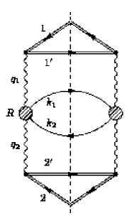
Figure 1: Cut diagram for lepton pair production from a two photon interaction. $R$ is the space-time point of the center of the collision region.

Figure 2: The diagrams that contribute, at lowest order, to the $\gamma\gamma\rightarrow e\bar{e}$ effective vertex.

As usual, we can rewrite Equation (1) in terms of Wigner transformed quantities. However, due to the photon fields interfering, the structure of the cross terms are complicated. The ${\left|S_{\rm 12\rightarrow 1^{\prime}2^{\prime}e\bar{e}}\right|}^{2}$ is:

$$\begin{array}[]{ccl}{\left|S_{\rm 12\rightarrow 1^{\prime}2^{\prime}e\bar{e}}\right|}^{2}&=&\alpha_{em}^{2}\displaystyle\int{d}^{4}R\>{d}^{4}r\>\frac{{d}^{4}k_{1}}{{(2\pi)}^{4}}\>\frac{{d}^{4}k_{2}}{{(2\pi)}^{4}}\>\frac{{d}^{4}q_{1}}{{(2\pi)}^{4}}\>\frac{{d}^{4}q_{2}}{{(2\pi)}^{4}}\>\frac{{d}^{4}p}{{(2\pi)}^{4}}\\ &&\displaystyle\times f(R-r/2,k_{1},R+r/2,k_{2})\\ &&\displaystyle\times\Lambda_{\mu\mu^{\prime}\nu\nu^{\prime}}(k_{1},k_{2},p,r)(2\pi)^{4}\delta^{4}\!\left(q_{1}+q_{2}-k_{1}-k_{2}\right)\\ &&\displaystyle\times\left\{(2\pi)^{4}\delta^{4}\!\left(q_{1}-k_{1}+p\right){A}^{\mu\mu^{\prime}}_{1}\!\left(R-r/2,q_{1}\right){A}^{\nu\nu^{\prime}}_{2}\!\left(R+r/2,q_{2}\right)\right.\\ &&\displaystyle+\left.(2\pi)^{4}\delta^{4}\!\left(q_{1}-k_{2}-p\right){A}^{\nu\nu^{\prime}}_{1}\!\left(R+r/2,q_{1}\right){A}^{\mu\mu^{\prime}}_{2}\!\left(R-r/2,q_{2}\right)\right.\\ &&\displaystyle+\left.\int{d}^{4}\tilde{r}\>\exp{[i\tilde{r}\cdot(-p+\frac{k_{1}-k_{2}}{2})-ir\cdot(q_{1}-q_{2})]}\right.\\ &&\displaystyle\times\left.{A}^{\nu\mu^{\prime}}_{1}\!\left(R-\tilde{r}/4,q_{1}\right){A}^{\mu\nu^{\prime}}_{2}\!\left(R+\tilde{r}/4,q_{2}\right)\right.\\ &&\displaystyle+\left.\int{d}^{4}\tilde{r}\>\exp{[i\tilde{r}\cdot(-p+\frac{k_{1}-k_{2}}{2})+ir\cdot(q_{1}-q_{2})]}\right.\\ &&\displaystyle\times\left.{A}^{\mu\nu^{\prime}}_{1}\!\left(R+\tilde{r}/4,q_{1}\right){A}^{\nu\mu^{\prime}}_{2}\!\left(R-\tilde{r}/4,q_{2}\right)\right\}\end{array}$$ (2)

This equation could look simpler if, in the interference terms, we Wigner transformed $A_{1}$ together with $A_{2}$. However then we would have a virtual electron being emitted by some interference field and then reabsorbed by another interference field and the resulting equations would be impossible to interpret using our photon distributions. In Equation (2), we neglect $\tilde{k}$ relative to $k$ in the effective vertex and in the factors of $(2k_{0}V)$ because the final state wave packets are sharply peaked in momentum. In Equation (2), $R$ is the center of the interaction points $x_{1}$ and $x_{2}$ and $r$ is the space-time separation of these points. The final state Wigner density is

$$\begin{array}[]{rl}\displaystyle f(x_{1},k_{1},x_{2},k_{2})=&\displaystyle\frac{1}{(2k_{1,0}V)}\frac{1}{(2k_{2,0}V)}\int\frac{{d}^{4}\tilde{k}_{1}}{{(2\pi)}^{4}}\>\frac{{d}^{4}\tilde{k}_{2}}{{(2\pi)}^{4}}\>e^{-i\tilde{k}_{1}x_{1}-i\tilde{k}_{2}x_{2}}\\ &\displaystyle\times f^{*}(k_{1}+\tilde{k}_{1}/2,k_{2}+\tilde{k}_{2}/2)f(k_{1}-\tilde{k}_{1}/2,k_{2}-\tilde{k}_{2}/2)\end{array}$$

and the Wigner transform of the effective vertex is

$$\Lambda_{\mu\mu^{\prime}\nu\nu^{\prime}}(k_{1},k_{2},p,r)=\int\frac{{d}^{4}\tilde{p}}{{(2\pi)}^{4}}\>e^{i\tilde{p}\cdot r}\Lambda_{\mu\nu}(k_{1},k_{2},p+\tilde{p}/2)\Lambda^{*}_{\mu^{\prime}\nu^{\prime}}(k_{1},k_{2},p-\tilde{p}/2).$$

We can write the effective vertex in terms of the scalar Feynman propagator,

$$\begin{array}[]{ccl}\Lambda_{\mu\mu^{\prime}\nu\nu^{\prime}}(k_{1},k_{2},p,r)&=&\bar{u}(k_{1},s_{1})\gamma_{\mu}(\not{\!p}+\frac{i}{2}\not{\!\partial}+m_{e})\gamma_{\nu}v(k_{2},s_{2})\\ &&\times\bar{v}(k_{2},s_{2})\gamma_{\nu^{\prime}}(\not{\!p}-\frac{i}{2}\not{\!\partial}+m_{e})\gamma_{\mu^{\prime}}u(k_{1},s_{1}){G}^{\rm c}\!\left(r,p\right)\\ &\equiv&\lambda_{\mu\mu^{\prime}\nu\nu^{\prime}}(k_{1},k_{2},p,r){G}^{\rm c}\!\left(r,p\right).\end{array}$$ (3)

We simplify the reaction probability by summing over the final state electron and positron spins. We simplify things even further by working in the ultra-relativistic limit, namely when $v_{1}^{2}\approx v_{2}^{2}\approx 0$. Under these approximations, we find

$$\begin{split}{\left|S_{\rm 12\rightarrow 1^{\prime}2^{\prime}e\bar{e}}\right|}^{2}=&\alpha_{em}^{2}\int{d}^{4}R\>{d}^{4}r\>\frac{{d}^{4}k_{1}}{{(2\pi)}^{4}}\>\frac{{d}^{4}k_{2}}{{(2\pi)}^{4}}\>\frac{{d}^{4}q_{1}}{{(2\pi)}^{4}}\>\frac{{d}^{4}q_{2}}{{(2\pi)}^{4}}\>\frac{{d}^{4}p}{{(2\pi)}^{4}}\>\\ &\times f(R-r/2,k_{1},R+r/2,k_{2})\\ &\times\sum_{\rm spins}\lambda_{\mu\mu^{\prime}\nu\nu^{\prime}}(k_{1},k_{2},p,r){G}^{\rm c}\!\left(r,p\right)(2\pi)^{4}\delta^{4}\!\left(q_{1}+q_{2}-k_{1}-k_{2}\right)\\ &\times\left\{(2\pi)^{4}\delta^{4}\!\left(q_{1}-k_{1}+p\right){A}^{\mu\mu^{\prime}}_{1}\!\left(R-r/2,q_{1}\right){A}^{\nu\nu^{\prime}}_{2}\!\left(R+r/2,q_{2}\right)\right.\\ &+\left.(2\pi)^{4}\delta^{4}\!\left(q_{1}-k_{2}-p\right){A}^{\nu\nu^{\prime}}_{1}\!\left(R+r/2,q_{1}\right){A}^{\mu\mu^{\prime}}_{2}\!\left(R-r/2,q_{2}\right)\right.\\ &+\left.2\int{d}^{4}\tilde{r}\>\cos{[\tilde{r}\cdot(-p+\frac{k_{1}-k_{2}}{2})-r\cdot(q_{1}-q_{2})]}\right.\\ &\times\left.{A}^{\nu\mu^{\prime}}_{1}\!\left(R-\tilde{r}/4,q_{1}\right){A}^{\mu\nu^{\prime}}_{2}\!\left(R+\tilde{r}/4,q_{2}\right)\right\}.\end{split}$$ (4)

Given the relatively simple form of this equation, one would think that we could identify the exchanged electron’s phase-space density. In fact, if we use free particle distributions for the final state electron and positron and sum over final states, we can identify the virtual electron distribution (Equation (21)) in the direct terms. However, we can not make the same identification in the interference term and factorization is not possible here. We might find factorization again if we had several point charges as one can envision a situation with many photon sources screening the photons (a plasma for instance). The photon field might then be an incoherent superposition of photon fields. In the absence of photon interference, we might be able to define an Effective Electron Distribution.

Appendix 10.B The $e\bar{e}$ Production Region vs. the Interaction Region

Even though Equation (4) does not factorize or acquire the “source-propagator” for any of the densities (except maybe the photon density), we can still figure out where the electron-positron pairs are produced and the size of the region where the two photons interact. We will see that the $e\bar{e}$ production region is set by the shape and size of the photon distributions and that the two photon interaction region’s size depends on the mass and virtuality of the exchanged electron.

First, take the virtual photon distribution of the classical point charge from Section 4. Now, the lowest energy and momentum that each of the interacting photons can have is $q=(m_{e},m_{e}/v_{L},\vec{0}_{T})$. Because the high energy or far off-shell photons are closer to the point charge then their lower energy and nearly on-shell cousins, photons with the minimum $q_{\mu}$ have the largest distributions. So, the geometrical overlap of the high energy portions of the virtual photon distribution sets the size of the $e\bar{e}$ production region. In Figure 3 we illustrate this: the two ellipses represent the edge of the photon distribution and the shaded region is the region where the $e\bar{e}$ pairs can be created.

Figure 3: Schematic of the pair production region. The ellipses represent the edge of the photon distributions, each with four-momentum $q=(m_{e},m_{e}/v_{L},\vec{0}_{T})$. The shaded region is the geometrical overlap of the photon distributions and sets the size of the $e\bar{e}$ production region. The arrows point in the direction of the photons’ source’s 3-momentum.

Now, the size of the two photon interaction itself is determined by how far the exchanged electron can travel between the vertices in Figure 2. For this, we look at the phase-space electron propagator. Assuming the electrons have mass, we use Remler’s causal propagator. Here the phase-space “probability” for propagating between two space-time points drops like $e^{-2m_{e}\tau}$ for space-like electrons and like $\sin{2\tau(\sqrt{p^{2}}\pm m_{e})}/(\sqrt{p^{2}}\pm m_{e})$ for time-like electrons. The proper time along the electron 4-momentum is $\tau$. In the direction transverse to the electron four-momentum, the “probability” is zero. Thus, the interaction region has a characteristic length scale of $\approx 1/m_{e}$. This is comparable to the width of the photon distributions, so there is no scale separation. Typically one requires the interaction length scale to be much smaller than the characteristic length scale of the particle density in order to justify the gradient expansions of the Quasi-Classical Approximation and allow for a transport description. Because our approach does not rely on the Quasi-Classical Approximation, the transport-like description in Chapter 1 is still be possible.

So, to summarize, we learned that the “source-propagator” picture of parton densities fails when the source particle and probe particle interact, even through quantum interference. Nevertheless, we can still discuss the process in phase-space with the phase-space sources and propagators, even if the densities have no clear meaning.

Chapter 11 WAVEPACKETS

Throughout this paper, we use wavepackets in the initial and final states of a reaction (or equivalently density matrices) to provide spatial localization or delocalization. In this appendix, we detail the construction of an initial or final state wavepacket and discuss the limits of either a completely localized or delocalized wavepacket.

Appendix 11.A On–Shell Gaussian Wavepacket

An initial (or final) state ket can be written with wavepackets:

$$\left|i\right>=\int\frac{{d}^{4}p}{{(2\pi)}^{4}}\>f(p)\left|\vec{p}\right>.$$ (1)

The corresponding Wigner function of the particles is

$$\begin{array}[]{rl}f(x,p)=&\displaystyle\int\frac{{d}^{4}p^{\prime}}{{(2\pi)}^{4}}\>e^{-ix\cdot p^{\prime}}\left<i\right|\hat{\phi}^{*}(p-p^{\prime}/2)\hat{\phi}(p+p^{\prime}/2)\left|i\right>\\ =&\displaystyle\frac{1}{2Vp_{0}}\int\frac{{d}^{4}p^{\prime}}{{(2\pi)}^{4}}\>e^{-x\cdot p^{\prime}}f(p+p^{\prime}/2)f^{*}(p-p^{\prime}/2).\end{array}$$ (2)

Particles in either the initial or final states are on–shell, so they can be expanded in momentum eigenstates. We choose the wavepacket to be a Gaussian superposition of momentum eigenstates with a momentum spread $\sigma$:

$$\phi(p)={\cal N}\delta\!\left(p^{2}-M^{2}\right)\exp{[-(\vec{p}-\vec{p}_{i})^{2}/2\sigma^{2}]}$$

The Wigner transform of this wavepacket can not be done analytically except in the limit when $|\vec{p}_{i}|\gg\sigma$. In this limit, $\vec{p}_{i}\approx\vec{p}\gg\vec{p^{\prime}}$ so our wavepacket is localized in momentum giving the following Wigner density of particles:

$$f(x,p)=\frac{|{\cal N}|^{2}}{8\pi p_{0}^{2}}\delta\!\left(p^{2}-M^{2}\right)\exp{\left[-\frac{(\vec{p}-\vec{p}_{i})^{2}}{2\sigma^{2}}\right]}(2\sigma\sqrt{2\pi})^{3}\exp{\left[-2\sigma^{2}(\vec{v}x_{0}-\vec{x})^{2}\right]}.$$ (3)

Here $\vec{v}=\vec{p}/p_{0}$ is the velocity of the wavepacket. Thus, the particle’s Wigner function is a Gaussian in both momentum and space. The spread in momentum is the inverse spread in space. The centroid of the Gaussian follows the particle’s classical trajectory. The magnitude of the energy of the packet is set by the delta function out front. We have not constrained the particle in energy so this density contains both positive and negative energy contributions.

Appendix 11.B Delocalizing the Wavepacket in Space: Free Wavepacket

In accordance with the uncertainty principle, the wavepacket becomes completely delocalized in space in the limit of complete localization in momentum (i.e. $\sigma\rightarrow 0$). In this limit, the spatial Gaussian approaches unity and the momentum Gaussian becomes a delta function. After working out the normalization, we have

$$f^{\rm free}(x,p)=\frac{1}{2Vp_{0}}(2\pi)^{4}\delta^{4}\!\left(p-p_{i}\right).$$ (4)

This is no surprise since the limit $\sigma\rightarrow 0$ squeezes the state into a momentum eigenstate. We use this result in Section 2 for the final state positron’s wavepacket.

Appendix 11.C Localizing the Wavepacket in Space: Classical Wavepacket

A classical particle is localized in both space and momentum, a seeming violation of the uncertainty principle. In real life, this is not a problem since the reason classical particles appear localized is that we probe them on length (or momentum) scales too coarse to resolve the interesting quantum features. In the case of our Gaussian wavepacket, this amounts to probing the distribution on length scales much larger than $1/\sigma$. In this case, the space Gaussian is too localized to resolve and we can replace it with a delta function. Additionally, if we assume that $\sigma$ is large, we can replace the momentum Gaussian with a delta function as well:

$$f^{\rm classical}(x,p)=\frac{1}{2}(2\pi)^{4}\delta^{3}\!\left(\vec{p}-\vec{p}_{i}\right)\delta\!\left(p^{2}-M^{2}\right)\delta^{3}\!\left(\vec{v}x_{0}-\vec{x}\right)$$ (5)

Here we have inserted the correct normalization for the wavepacket. This density corresponds to an on-mass-shell particle that follows its classical trajectory $\vec{v}x_{0}=\vec{x}$. Again, we left in both positive and negative energy contributions. We use the result (5) in the next appendix to find the current of a classical point charge.

Chapter 12 THE CURRENT DUE TO A CLASSICAL PARTICLE

In this appendix, we derive the classical current used in the Effective Photon Distribution calculation of Chapter 2. For the sake of illustration, we take the point particle to be a scalar particle. The derivation takes three steps: first we define the Wigner current of a scalar particle, then we derive the photon/scalar interaction vertex in phase-space, and finally we localize the initial and final states of the scalar to give the classical current.

Appendix 12.A Wigner Current

We begin by restating Equation (3):

$${J}^{\mu\nu}_{\rm A}\!\left(x,q\right)=\int\frac{{d}^{4}\tilde{q}}{{(2\pi)}^{4}}\>e^{-i\tilde{q}\cdot x}\left<A^{\prime}\right|j^{\mu}(q+\tilde{q}/2)\left|A\right>\left<A\right|j^{\dagger\nu}(q-\tilde{q}/2)\left|A^{\prime}\right>.$$ (1)

We write the initial and final state bra’s and ket’s according to Equation (2) and rewrite Equation (1) in terms of initial and final Wigner densities,

$${J}^{\mu\nu}_{\rm A}\!\left(x,q\right)=\int\frac{{d}^{4}p_{i}}{{(2\pi)}^{4}}\>\frac{{d}^{4}p_{f}}{{(2\pi)}^{4}}\>{f}_{A}\left(x,p_{i}\right){f}^{*}_{A^{\prime}}\left(x,p_{f}\right)(2\pi)^{4}\delta^{4}\!\left(p_{i}-p_{f}-q\right)\Gamma_{\mu\nu}(q,p_{i},p_{f}).$$ (2)

We assume that the initial and final wavepackets are localized in momentum and some-what delocalized in space. Shortly, we will also assume that we probe this current on length scales much larger than even this delocalized space distribution.

Appendix 12.B Scalar Vertex

$\Gamma_{\mu\nu}(q,p_{i},p_{f})$ is not quite the Wigner transform of the $\gamma AA^{\prime}$ vertex, although it does arise from performing the Wigner transform in Equation (1). It is defined by

$$\begin{split}\@ADDCLASS{ltx_eqn_lefteqn}$\displaystyle(2\pi)^{4}\delta^{4}\!\left(p_{i}-p_{f}-q\right)\Gamma_{\mu\nu}(q,p_{i},p_{f})=$\mbox{}\hfil\hskip 30.00005pt&\\ &4V^{2}p_{f}^{0}p_{i}^{0}\int\frac{{d}^{4}\tilde{q}}{{(2\pi)}^{4}}\>\left<\vec{p}_{f}\right|j_{\mu}(q+\tilde{q}/2)\left|\vec{p}_{i}\right>\left<\vec{p}_{i}\right|j^{\dagger}_{\nu}(q-\tilde{q}/2)\left|\vec{p}_{f}\right>\end{split}$$ (3)

Using the matrix element

$$\left<\vec{p}_{f}\right|j_{\mu}(q)\left|\vec{p}_{i}\right>=eZ(2\pi)^{4}\delta^{4}\!\left(p_{i}-p_{f}-q\right)\frac{(p_{i}+p_{f})_{\mu}}{2V\sqrt{p_{f}^{0}p_{i}^{0}}},$$

We find

$$\Gamma_{\mu\nu}(q,p_{i},p_{f})=\alpha_{em}Z^{2}(p_{i}+p_{f}+\frac{1}{2}(\tilde{p_{i}}+\tilde{p_{f}}))_{\mu}(p_{i}+p_{f}-\frac{1}{2}(\tilde{p_{i}}+\tilde{p_{f}}))_{\nu}$$ (4)

The relative momenta, $\tilde{p}_{i}$ and $\tilde{p}_{f}$, become derivatives on $x$ in the current (2). Assuming the wavepackets to be uniform the the reaction’s length scales, we can ignore the derivatives and arrive at the phase-space scalar vertex

$$\Gamma_{\mu\nu}(q,p_{i},p_{f})=\alpha_{em}Z^{2}(p_{i}+p_{f})_{\mu}(p_{i}+p_{f})_{\nu}.$$ (5)

Appendix 12.C Classical Current

We are now in a position to derive Equation (14) for the classical current density in phase-space. First, we take the final state to be a momentum eigenstate and sum over it. Since the final state is localized in momentum around $p_{f}$, this is not a bad approximation. Second, we take the initial state to be a classical wavepacket. In other words, we assume that the initial state is localized in momentum and delocalized in space but that we probe it on such large length scales that we still see a spatially localized wavepacket. So, putting Equations (4), (5) and (5) into (2) and summing over final states, we get

$${J}^{\mu\nu}\!\left(x,q\right)=2\pi\alpha_{em}Z^{2}\>v_{\mu}v_{\nu}\>\delta^{3}\!\left(\vec{x}-x_{0}\vec{v}\right)p_{i0}\delta((p_{f}+q)^{2}-M^{2}).$$

Using $p_{f}^{2}=M^{2}$ and $v_{\mu}\approx p_{f\mu}/p_{i0}$ and assuming $q^{2}/p_{i0}\ll q\cdot v$, we get the classical current:

$${J}^{\mu\nu}_{\rm classical}\!\left(x,q\right)=2\pi\alpha_{em}Z^{2}\>v_{\mu}v_{\nu}\>\delta(q\cdot v)\delta^{3}\!\left(\vec{x}-x_{0}\vec{v}\right).$$ (6)

Note that this current allows for emission of both positive and negative energy photons. In Section 1, we restrict emission to positive energy photons by inserting a factor of $\theta(q_{0})$ in Equation (6). This can be justified by suitably choosing $\vec{p}_{f}$ and $\vec{p}_{i}$ and restricting the initial and final states to have only positive energy.

REFERENCES

REFERENCES

- [AB65] A. I. Akhiezer and V. B. Berestetskii. Quantum Electrodynamics. Wiley Interscience, New York, 1965.
- [AHC95] S. Aid (H1 Collaboration). Transverse energy and forward jet production in the low x regime at HERA. Phys. Lett. B, 356:118, 1995.
- [AP77] G. Altarelli and G. Parisi. Asymptotic freedom in parton language. Nucl. Phys. B, 126:298, 1977.
- [B+80] M. Bertero et al. The stability of inverse problems. In H. P. Baltes, editor, Inverse Scattering Problems in Optics, Topics in Current Physics, page 161. Springer, Berlin, 1980.
- [B+85] W. M. Boerner et al., editors. Inverse Methods in Electromagnetic Imaging, volume 143 of NATO Advanced Study Institute, Series C: Mathematical & Physical Sciences. Reidel, Dordrecht, 1985.
- [B+97] S. A. Bass et al. Are we close to the QGP? – Hadrochemical vs. microscopic analysis of particle production in ultrarelativistic heavy ion collisions. [Online] Available http://xxx.lanl.gov/nucl-th/9711032, November 1997.
- [Bal80] H. P. Baltes, editor. Inverse Scattering Problems in Optics, Topics in Current Physics. Springer, Berlin, 1980.
- [Bay98] Gordon Baym. The physics of Hanbury Brown–Twiss intensity interferometry: from stars to nuclear collisions. Acta Phys. Polon. B, 29:1839–1884, 1998.
- [BB88] C. A. Bertulani and G. Baur. Electromagnetic processes in relativistic heavy ion collisions. Phys. Rep., 163:299, 1988.
- [BBM96] G. Baym and P. Braun-Munzinger. Physics of Coulomb correction in Hanbury Brown–Twiss interferometry in ultrarelativistic heavy ion collisions. Nucl. Phys. A, 610:286c–296c, 1996.
- [BD72] B. Bezzerides and D. F. DuBois. Quantum electrodynamics of nonthermal relativistic plasmas: Kinetic theory. Ann. Phys., 70:10–66, 1972.
- [BD97] David A. Brown and Paweł Danielewicz. Imaging of sources in heavy-ion reactions. Phys. Lett. B, 398:252–258, 1997.
- [BD98a] David A. Brown and Paweł Danielewicz. Optimized discretization of sources imaged in heavy-ion reactions. Phys. Rev. C, 57(5):2474–2483, May 1998.
- [BD98b] David A. Brown and Paweł Danielewicz. Partons in phase-space. Phys. Rev. D, 1998. In press.
- [BEC97] J. Barrette (E877 Collaboration). Two pion correlations in Au+Au at GeV/c per nucleon. Phys. Rev. Lett., 78:2916–2919, 1997.
- [Ber94] George Bertsch. Meson phase space density in heavy-ion collisions from interferometry. Phys. Rev. Lett, 72(15):2349–2350, 1994.
- [Ber96] George Bertsch. Meson phase space density in heavy-ion collisions from interferometry. Phys. Rev. Lett, 77:789, 1996.
- [Bev85] R. M. Bevensee. Maximum Entropy Methods in Electromagnetic/Geophysical/Ultrasonic imaging. In W. M. Boerner et al., editors, Inverse Methods in Electromagnetic Imaging, volume 143 of NATO Advanced Study Institute, Series C: Mathematical & Physical Sciences, page 375. Reidel, Dordrecht, 1985.
- [BG67] G. E. Backus and F. Gilbert. Numerical applications of a formalism for geophysical inverse problems. Geophys. J. (GB), 13(1–3):247–276, 1967. Proceedings of Third International Symposium on Geophysical Theory and Computers, Cambridge 1966.
- [BGJ90] D. H. Boal, G. K. Gelbke, and B. K. Jennings. Intensity interferometry in subatomic physics. Rev. Mod. Phys., 62:553, 1990.
- [BGMS75] V. M. Budnev, I. F. Ginzburg, G. V. Meledin, and V. G. Serbo. The two–photon particle production method. Physics problems. Applications. Effective Photon Approximation. Phys. Rep., 15:181, 2821975.
- [BI94] Jean-Paul Blaizot and Edmond Iancu. Soft collective excitations in hot gauge theories. Nucl. Phys. B, 417:608–673, 1994.
- [BL78] Ya. Ya. Balitskii and L. N. Lipatov. Pomeranchuk singularity in quantum chromodynamics. Yad. Fiz., 28(6):1597–1611, 1978. [Sov. J. Nucl. Phys. 28:822 (1978)].
- [BL93] J. Bartels and H. Lotter. A note on the BFKL pomeron and the “hot spot” cross section. Phys. Lett. B, 309:400–408, 1993.
- [BS79] N. N. Bogoliubov and D. V. Shirkov. Introduction to the Theory of Quantized Fields. John Wiley and Sons, New York, 1979.
- [CMV81] J. Cugnon, T. Mizutani, and J. Vandermeulen. Equilibration in relativistic nuclear collisions. A Monte Carlo calculation. Nucl. Phys. A, 352:505, 1981.
- [Coc74] G. Cocconi. Second-order interference as a tool for the determination of hadron fireball dimensions. Phys. Lett. B, 49(5):459–461, 1974.
- [CSHY85] Kuang-chao Chou, Zhao-bin Su, Bai-lin Hao, and Lu Yu. Equilibrium and nonequilibrium formalisms made unified. Phys. Rep., 118:1–131, 1985.
- [Cug82] J. Cugnon. Internuclear Cascade Model. A review. Nucl. Phys. A, 387:191–203, 1982.
- [CZ83] P. Carruthers and F. Zachariasen. Quantum collision theory with phase–space distributions. Rev. Mod. Phys., 55:245–285, 1983.
- [D+91] Y. L. Dokshitzer et al. Basics of Perturbative QCD. Editions Frontiéres, Gif-sur-Yvette, France, 1991.
- [D’A95] G. D’Agostini. Probability and measurement uncertainty in physics: A Bayesian primer. [Online] Available http://xxx.lanl.gov/hep-ph/9512295, December 1995.
- [Dan84] Paweł Danielewicz. Quantum theory of nonequilibrium processes, I. Ann. Phys., 152(2):239–304, February 1984.
- [Dan90] Paweł Danielewicz. Operator expectation values, self-energies, cutting rules and higher–order processes in quantum many-body theory. Ann. Phys., 197:154–201, 1990.
- [Dan95] Paweł Danielewicz. Effects of compression and collective expansion on particle emission from central heavy ion reactions. Phys. Rev. C, 51:716–750, 1995.
- [DB91] P. Danielewicz and G. F. Bertsch. Production of deuterons and pions in a transport model of energetic heavy–ion reactions. Nucl. Phys. A, 533:712–748, 1991.
- [DB98] Paweł Danielewicz and David Brown. Neutron-proton correlations near the Coulomb barrier. In preparation, 1998.
- [DeT95] Carleton DeTar. Quark Gluon Plasma in numerical simulations of lattice QCD. In Rudolph Hwa, editor, Quark–Gluon Plasma 2, chapter 1, pages 1–55. World Scientific, New York, 1995.
- [dH80] F. R. de Hoog. Review of Fredholm equations of the first kind. In R. S. Anderssen et al., editors, The Application and Numerical Solution of Integral Equations, page 119. Sijthoff & Noordhoff, Alphen aan den Rijn, 1980.
- [DS92] Paweł Danielewicz and Peter Schuck. Formation of particle correlation and cluster production in heavy-ion-induced reactions. Phys. Lett. B, 274:268–274, 1992.
- [EGV86a] H. Elze, M. Gyulassy, and D. Vasak. Transport equation for the QCD gluon Wigner operator. Nucl. Phys. B, 177:402–408, 1986.
- [EGV86b] H. Elze, M. Gyulassy, and D. Vasak. Transport equation for the QCD quark Wigner operator. Nucl. Phys. B, 276:706–728, 1986.
- [EW93] K. J. Eskola and X.-N. Wang. Space–time evolution of semihard QCD-quanta in ultrarelativistic heavy–ion collisions. In Proceedings of the Workshop on Pre–Equilibrium Parton Dynamics, pages 49–60, Berkeley, CA, 1993.
- [Fie89] Richard Field. Applications of Perturbative QCD. Frontiers in Physics Lecture Note Series. Addison-Wesley, 1989.
- [FW71] Alexander L. Fetter and John D. Walecka. Quantum Theory of Many–Particle Systems. McGraw–Hill, 1971.
- [G+59] G. Goldhaber et al. Pion-pion correlations in antiproton annihilation events. Phys. Rev. Lett., 3:181–183, 1959.
- [G+90] W. G. Gong et al. Intensity interferometry test of nuclear collision geometries obtained from Boltzmann-Uehling-Uhlenbeck equation. Phys. Rev. Lett., 65:2114–2117, 1990.
- [G+91] W. G. Gong et al. Space-time evolution of the reaction 14NAl, 197Au at E/A= MeV and 197XeAl, 122Sn at E/A MeV probed using two proton intensity interferometry. Phys. Rev. C, 43:1804–1820, 1991.
- [G+93] W. G. Gong et al. Two–deuteron correlation functions in 14NAl at E/A MeV. Phys. Rev. C, 47:R429–R430, 1993.
- [G+95] S. Gaff et al. Two-proton correlations for 16OAu collision at E/A MeV. Phys. Rev. C, 52:2782–2784, 1995.
- [Gei92a] Klaus Geiger. Thermalization in ultrarelativistic collisions. 1. Parton kinetics and Quark Gluon Plasma formation. Phys. Rev. D, 46:4965–4985, 1992.
- [Gei92b] Klaus Geiger. Thermalization in ultrarelativistic collisions. 2. Entropy production and energy density at RHIC and LHC. Phys. Rev. D, 46:4986–5005, 1992.
- [Gei94] Klaus Geiger. Probing the space-time structure of quark and gluon transport in proton–nucleus collisions at collider energies. Phys. Rev. D, 49(6):3234–3252, 1994.
- [Gei95] Klaus Geiger. Space-time description of ultrarelativistic nuclear collisions in the QCD parton picture. Phys. Rep., 258:237–376, 1995.
- [Gei96] Klaus Geiger. Quantum field kinetics of QCD: Quark-gluon transport theory for light–cone dominated processes. Phys. Rev. D, 54:949–988, 1996.
- [GGLP60] G. Goldhaber, S. Goldhaber, W. Lee, and A. Pais. Influence of Bose-Einstein statistics on the antiproton-proton annihilation process. Phys. Rev., 120:300, 1960.
- [GK93] Klaus Geiger and J. Kapusta. Chemical equilibration of partons in high energy nuclear collisions. Phys. Rev. D, 47:4905–4919, 1993.
- [GKP71] V. G. Grishin, G. I. Kopylov, and M. I. Podgoretskii. Interference of identical particles in processes with excited nuclei. Yad. Fiz., 13(5):1116–1125, 1971. [Sov. J. Nucl. Phys. 13, 638 (1971)].
- [GLR83] L. V. Gribov, E. M. Levin, and M. G. Ryskin. Semihard processes in QCD. Phys. Rep., 100:1–150, 1983.
- [GR94] I. S. Gradshteyn and I. M. Ryzhik. Table of Integrals, Series, and Products. Academic Press, San Diego, edition, 1994.
- [H+95] D. Handzy et al. Understanding proton emission in central heavy-ion collisions. Phys. Rev. Lett., 75:2916–2919, 1995.
- [H+96] T. M. Hamilton et al. Changing source characteristics during multifragment decay. Phys. Rev. C., 53:2273–2286, 1996.
- [Had23] J. Hadamard. Lectures on the Cauchy Problem in Linear Partial Differential Equations. Yale University Press, New Haven, 1923.
- [Hag65] R. Hagedorn. Statistical thermodynamics of strong interactions at high energies. Suppl. Nuovo Cimento, 3:147–186, 1965.
- [Hag68] R. Hagedorn. Statistical thermodynamics of strong interactions at high energies. III. Heavy-pair (quark) production rates. Suppl. Nuovo Cimento, 6:311–354, 1968.
- [Hag71] R. Hagedorn. Thermodynamics of the strong interaction. Technical Report CERN report No. 71-12, CERN, Geneva, 1971.
- [HBFZ96] P. A. Henning, M. Blasone, R. Fauser, and P. Zhuang. Thermalization of a quark gluon plasma. [Online] Available http://xxx.lanl.gov/hep-ph/9612492, November 1996. Submitted to Phys. Rev. D.
- [HBJDG52] R. Hanbury-Brown, R. C. Jennison, and M. K. Das Gupta. Apparent angular sizes of discrete radio sources. Observations at Jodrell Bank, Manchester. Nature, 170:1061–1065, December 1952.
- [HBT54] R. Hanbury-Brown and R. Q. Twiss. A new type of interferometer for use in radio astronomy. Phil. Mag., 45:633–682, July 1954.
- [HBT56a] R. Hanbury-Brown and R. Q. Twiss. Nature, 178:1046, 1956.
- [HBT56b] R. Hanbury-Brown and R. Q. Twiss. Correlation between photons in two coherent beams of light. Nature, 177:27–28, 1956.
- [HBT56c] R. Hanbury-Brown and R. Q. Twiss. The question of correlation between photons in coherent light rays. Nature, 178:1447, 1956.
- [HBT57a] R. Hanbury-Brown and R. Q. Twiss. Interferometry of the intensity fluctuations in light. I. Basic theory. The correlation between photons in coherent beams of radiation. Proc. R. Soc. A, 242:300–324, 1957.
- [HBT57b] R. Hanbury-Brown and R. Q. Twiss. Interferometry of the intensity fluctuations in light. II. An experimental test of the theory for partially coherant light. Proc. R. Soc. A, 243:291–319, 1957.
- [Hen95] P. A. Henning. Quantum transport: Beyond molecular dynamics. In Procedings of the International Workshop on Thermal Field Theories, Dalian, China, 1995.
- [HM96] John Harris and Berndt Müller. The search for the Quark Gluon Plasma. Ann. Rev. Nucl. Part. Sci., 46:71, 1996.
- [IZ80] Claude Itzykson and Jean-Bernard Zuber. Quantum Field Theory. McGraw–Hill, Inc., New York, 1980.
- [Jac75] J. D. Jackson. Classical Electrodynamics. John Wiley and Sons, New York, 1975.
- [KB62] Leo Kadanoff and Gordon Baym. Quantum Statistical Mechanics (Green’s Function Methods in Equilibrium and Nonequilibrium Problems). W. A. Benjamin, Inc., New York, 1962.
- [KBH+95] Gerd Kortemeyer, Wolfgang Bauer, Kevin Haglin, Joelle Murray, and Scott Pratt. Causality violations in cascade models of nuclear collisions. Phys. Rev. C, 52(5):2714–2724, November 1995.
- [KIV98] Jörn Knoll, Yu. B. Ivanov, and Dmitri N. Voskresensky. Towards a quantum transport description of particles with finite mass width. [Online] Available http://xxx.lanl.gov/hep-ph/9809419, September 1998.
- [KLF76] E. A. Kurayev, L. N. Lipatov, and V. S. Fadin. Multireggeon processes in the Yang-Mills theory. Zh. Exsp. Teor. Fiz., 71(3):840–855, 1976. [Sov. Phys. JETP 44:443 (1976)].
- [KLF77] E. A. Kurayev, L. N. Lipatov, and V. S. Fadin. Pomeranchuk singularity in non-Abelian gauge theories. Zh. Exsp. Teor. Fiz., 72(2):377–389, 1977. [Sov. Phys. JETP 45:199 (1977)].
- [KLW87] C. M. Ko, Q. Li, and R. Wang. Relativistic Vlasov equation for heavy ion collisions. Phys. Rev. Lett, 59(10):1084–1087, 1987.
- [KOH97] S. Klevansky, A. Ogura, and J. Hüfner. Derivation of transport equations for a strongly interacting Lagrangian in powers of and . Ann. Phys., 261:37, 1997.
- [Kop72] G. I. Kopylov. Possibilities of resonance interferometry. Yad. Fiz., 15(1):178–186, 1972. [Sov. J. Nucl. Phys. 15, 103 (1972)].
- [Kop74] G. I. Kopylov. Like particle correlations as a tool to study the multiple production mechanism. Phys. Lett. B, 50:472–474, 1974.
- [KP71] G. I. Kopylov and M. I. Podgoretskii. Interference effects on two-resonance systems. Yad. Fiz., 14(5):1081–1090, 1971. [Sov. J. Nucl. Phys. 14, 604 (1972)].
- [KP72] G. I. Kopylov and M. I. Podgoretskii. Correlations of identical particles emitted by highly excited nuclei. Yad. Fiz., 15(2):392, 1972. [Sov. J. Nucl. Phys. 15, 219 (1972)].
- [KP73] G. I. Kopylov and M. I. Podgoretskii. Multiple production and interference of particles emitted by moving sources. Yad. Fiz., 18(3):656–666, 1973. [Sov. J. Nucl. Phys. 18, 336 (1973)].
- [KPM97] Ch. Kurtsiefer, T. Pfau, and J. Mlynek. Measurement of the Wigner function of an ensemble of helium atoms. Nature, 386:150–153, 1997.
- [KV96] Jörn Knoll and Dmitri N. Voskresensky. Classical and quantum many-body description of bremsstrahlung in dense matter; Landau-Pomeranchuk-Migdal effect. Ann. Phys., 249:532–581, 1996.
- [Lan77] P. Landshoff. The transverse momentum of partons. Phys. Lett. B, 66(5):452–454, February 1977.
- [Lee95] Hai-Woong Lee. Theory and application of the quantum phase–space distribution functions. Phys. Rep., 259:147–211, 1995.
- [Leh59] H. Lehmann. Scattering matrix and field operators. Supp. del Nuovo Cimento, 14(1):153–176, 1959.
- [Lip76] L. N. Lipatov. Reggeization of the vector meson and the vacuum singularity in non–Abelian gauge theories. Yad. Fiz., 23:642, 1976. [Sov. J. Nucl. Phys. 23:338 (1976)].
- [LL94] E. Laenen and E. Levin. Parton densities at high density. Ann. Rev. Nucl. Part. Sci., 44:199–246, 1994.
- [Lur68] David Lurié. Particles and Fields. Interscience Publishers, John Wiley and Sons, New York, 1968.
- [Lyn98] W. Lynch. Fragmentation and multifragmentation in nuclear collisions. Rev. Mod. Phys., 1998. To be published.
- [Mak95a] A. Makhlin. Quantum field kinetics. Phys. Rev. C, 51(6):3454–3464, June 1995.
- [Mak95b] A. Makhlin. Quark and gluon distributions at the earliest stage of heavy–ion collisions. Phys. Rev. C, 52(2):995–1021, August 1995.
- [Mak96] A. Makhlin. Spurious poles of the axial gauge propagators and dynamics of the interacting fields. [Online] Available http://xxx.lanl.gov/hep-ph/9608260, August 1996.
- [McL86] Larry McLerran. The physics of the Quark Gluon Plasma. Rev. Mod. Phys., 58(4):1021–1064, 1986.
- [McL97] Larry McLerran. Small x physics and why it’s interesting. [Online] Available http://xxx.lanl.gov/hep-ph/9705426v1, May 1997.
- [MD90] Stanisław Mrówczyński and Paweł Danielewicz. Green function approach to transport theory of scalar fields. Nucl. Phys. B, 342:345–380, 1990.
- [MEC96] D. Miśkowiec (E877 Collaboration). Two-particle correlations in Au-Au collisions at AGS energy. Nucl. Phys. A, 610:227c–239c, 1996.
- [MH94] Stanisław Mrówczyński and Ulrich Heinz. Towards relativistic transport theory of nuclear matter. Ann. Phys., 229:1–54, 1994.
- [MS86] T. Matsui and H. Satz. J suppression by quark-gluon plasma formation. Phys. Lett. B, 178(4):416–422, 1986.
- [MS98] A. Makhlin and E. Surdutovich. Scenario for ultrarelativistic nuclear collisions: Space–time picture of quantum fluctuations and the birth of QGP. Phys. Rev. C, 58(1):389, 1998.
- [Mue89] A. H. Mueller. QCD and relativistic heavy–ion collicions. Nucl. Phys. A, 498:41c–52c, 1989.
- [Mül85] Berndt Müller. The Physics of the Quark Gluon Plasma. Springer–Verlag, Berlin, 1985.
- [NCK98] S. Nickerson, T. Csörgő, and D. Kiang. Testing the core-halo model on Bose-Einstein correlation functions. Phys. Rev. C, 57:3251–3262, 1998.
- [NR86] Y. P. Nikitin and I. L. Rozental. High Energy Physics with Nuclei. Harwood Academic Publishers, New York, 1986.
- [P+92] W.H. Press et al. Numerical Recipes: The Art of Scientific Computation. Cambridge University Press, Cambridge, 1992.
- [PCZ90] S. Pratt, T. Csörgő, and J. Zimányi. Detailed predictions for two-pion correlations in ultrarelativistic heavy-ion collisions. Phys. Rev. C, 42(6):2646–2652, December 1990.
- [Qui83] Chris Quigg. Gauge Theories of the Strong, Weak, and Electromagnetic Interactions. Frontiers in Physics Lecture Note Series. Addison-Wesley, 1983.
- [R+96] D. Rischke et al. Hydrodynamics and collective behavior in relativistic nuclear collisions. In Structure of Vacuum Elementary Matter, pages xxxi,711, 555–562, Wilderness, South Africa, March 1996. International Conference on Nuclear Physics at the Turn of the Millennium, World Scientific.
- [Raj95] K. Rajagopal. The Chiral phase transition in QCD: Critical phenomina and long wavelength pion oscillations. In Rudolph Hwa, editor, Quark–Gluon Plasma 2, chapter 9, pages 484–554. World Scientific, New York, 1995.
- [Rem86] E. A. Remler. Phase–space calculations of composite particle production. In The physics of phase space: nonlinear dynamics and chaos, geometric quantization, and Wigner function, pages 214–221, University of Maryland, College Park, MD, May 1986. First International Conference on the Physics of Phase Space, Springer–Verlag.
- [Rem90] E. A. Remler. Simulation of multiparticle scattering. Ann. Phys., 202:351–397, 1990.
- [RG96a] Dirk Rischke and M. Gyulassy. The maximium lifetime of the quark–gluon plasma. Nucl. Phys. A, 597(4):701–726, 1996.
- [RG96b] Dirk Rischke and M. Gyulassy. The time–delay signature of quark–gluon plasma formation in relativistic nuclear collisions. Nucl. Phys. A, 608(4):479–512, 1996.
- [Ris96] Dirk Rischke. Hydrodynamics and collective behavior in relativistic nuclear collisions. Nucl. Phys. A, 610:88c–101c, December 1996.
- [Ris97] Dirk Rischke. Time delay and flow signatures of the QCD phase transition. In H. Feldmeier, J. Knoll, W. Noerenberg, and J. Wambach, editors, QCD Phase Transitions, pages 339–348, Hirschegg, Austria, January 1997. International Workshop XXV on Gross Properties of Nuclei and Nuclear Excitations.
- [RNC98] Albert Romana (NA50 Collaboration). The search for the Quark–Gluon Plasma: Study of production of charmed bound states in Pb–Pb collisions at GeV/Nucleon. XXXIIIrd Recontres de Moriond, Les Arcs, France, March 1998.
- [RPM+95] Dirk Rischke, Y. Pursun, J. A. Maruhn, H. Stocker, and W. Greiner. The phase transition to the quark–gluon plasma and its effect on hydrodynamic flow. Acta Phys. Hung., 1(3-4):309–322, 1995.
- [RS86] Jørgen Rammer and H. Smith. Quantum field-theoretical methods in transport theory of metals. Rev. Mod. Phys., 58(2):323–359, 1986.
- [S+93] J. P. Sullivan et al. Bose-Einstein correlations of pion pairs and kaon pairs from Relativistic Quantum Molecular Dynamics. Phys. Rev. Lett., 70(20):3000–3003, May 1993.
- [S+94] V. G. J. Stoks et al. Construction of high quality nucleon nucleon potential models. Phys. Rev. C, 49:2950–2962, 1994.
- [SBH+91] H. Sorge, M. Berenguer, C. Hartnack, A. von Keitz, R. Mattiello, G. Peilert, H. Stöcker, and W. Greiner. Microscopic dynamics of relativistic heavy ion collisions – probing extreme states of nuclear matter. In L. P. Csernai and D. D. Strottman, editors, Relativistic Heavy Ion Physics, volume 6 of International Review of Nuclear Physics, chapter 9, pages 641–717. World Scientific, New York, 1991.
- [SCC95] G. Sterman (CTEQ Collaboration). Handbook of perturbative QCD. Rev. Mod. Phys., 67:157, 1995.
- [Sch61] Julian Schwinger. Brownian motion of a quantum oscillator. J. Math. Phys., 2:407–432, 1961.
- [Sch94] H. Schoeller. A new transport equation for single-time Green’s functions in an arbitrary quantum system. General formalism. Ann. Phys., 229:273–319, 1994.
- [Ser47] R. Serber. Nuclear reactions at high energy. Phys. Rev., 72:1114–1115, 1947.
- [SG85a] J. Skilling and S. F. Gull. Algorithms and applications. In C. R. Smith and W. T. Grandy, editors, Maximum Entropy and Bayesian Methods in Inverse Problems, Fundamental Theories of Physics, page 83. Reidel, Dordrecht, 1985.
- [SG85b] C. R. Smith and W. T. Grandy, editors. Maximum Entropy and Bayesian Methods in Inverse Problems. Fundamental Theories of Physics. Reidel, Dordrecht, 1985.
- [Shu73a] E. V. Shuryak. The correlations of identical pions in multibody production (Pomeranchuk model). Phys. Lett. B, 44(4):387–389, 1973.
- [Shu73b] E. V. Shuryak. Correlations of identical pions in multiple production reactions. Yad. Fiz., 18(6):1302–1308, 1973. [Sov. J. Nucl. Phys. 18: 667 (1973)].
- [Ste93] George Sterman. An Introduction to Quantum Field Threory. Cambridge University Press, New York, 1993.
- [SV93] Mikolaj Sawicki and James Vary. Off-shell partons, Gottfried sum rule, and dilepton suppression. Phys. Rev. Lett., 71(9):1320–1323, August 1993.
- [Tat83] V. I. Tatarskii. The Wigner representation of quantum mechanics. Sov. Phys.–Usp., 26:311–327, 1983.
- [Tik63] A. N. Tikhonov. Solution of incorrectly formulated problems and the regularization method. Sov. Math. Dokl., 4:1035–1038, 1963.
- [TW94] W. K. Tung and H. Weerts. Summer school on QCD analysis and phenomenology. Lake Ozark, Missouri, 1994.
- [Ven95] Raju Venugopalan. Wee partons in large nuclei: from virtual dream to hard reality. Nucl. Phys. A, 590:147c–162c, 1995.
- [VGE87] D. Vasak, M. Gyulassy, and H. Elze. Quantum transport theory for Abelian plasmas. Ann. Phys., 173:462–492, 1987.
- [VL93] Y. Vardi and D. Lee. From image deblurring to optimal investments: Maximum Likelihood solutions for positive linear inverse problems. J. R. Stat. Soc. B, 55(3):569–612, 1993.
- [Von98] T. Vongpaseuth. Two-particles correlations from central Au+Au collisions at the AGS at BNL. Czech. J. of Phys., Suppl. S1, 48, 1998. RHIP ’97 Proceedings.
- [vW34] C. F. von Weizsäcker. Ausstrahlung bei Stössen sehr schneller Elektronen. Z. Phys., 88:612, 1934.
- [Wan95] X.-N. Wang. Approach to parton equilibration. Nucl. Phys. A, 590:47c–62c, 1995.
- [Web98] Henning Webber. QMD Movies. [Online] Available http://www.th.physik.uni-frankfurt.de/weber/Movies/index.html, July 1998.
- [WG91] X.-N. Wang and M. Gyulassy. HIJING: a Monte Carlo model for multiple jet production in pp, pA and AA collisions. Phys. Rev. D, 44:3501–3516, 1991.
- [WG92] X.-N. Wang and M. Gyulassy. A systematic study of particle production in p+p (anti p) collisions via the HIJING model. Phys. Rev. D, 45:844–856, 1992.
- [WH96] Urs A. Wiedemann and Ulrich Heinz. A new class of Hanbury-Brown/Twiss parameters. [Online] Available http://xxx.lanl.gov/nucl-th/9610043, October 1996.
- [Wil34] E. J. Williams. Nature of the high energy particles of penetrating radiation and states of ionization and radiation formulae. Phys. Rev., 45:729, 1934.
- [ZH96] P. Zhuang and U. Heinz. Relativistic quantum transport theory for electrodynamics. Ann. Phys., 245:311–338, 1996.