Abstract

We discuss renormalization of the non-relativistic three-body problem with short-range forces. The problem is non-perturbative at momenta of the order of the inverse of the two-body scattering length. An infinite number of graphs must be summed, which leads to a cutoff dependence that does not appear in any order in perturbation theory. We argue that this cutoff dependence can be absorbed in one local three-body force counterterm and compute the running of the three-body force with the cutoff. This allows a calculation of the scattering of a particle and the two-particle bound state if the corresponding scattering length is used as input. We also obtain a model-independent relation between binding energy of a shallow three-body bound state and this scattering length. We comment on the power counting that organizes higher-order corrections and on relevance of this result for the effective field theory program in nuclear and molecular physics.

I Introduction

The three-body system provides non-trivial testground for ideas developed in two-body dynamics, and as such has a long and venerable history. It is in general of very difficult solution, but when all particles have momenta much smaller than the inverse of the range of interactions it simplifies considerably while still retaining some very rich universal features [1, 2, 3]. At such low energies, the two-body system can be attacked with many different techniques: effective range expansion, boundary conditions at the origin, etc.; a particularly convenient method for the extension to a many-body context is that of effective field theory (EFT) [4]. Here we use EFT to solve the three-body system with short-range interactions in a systematic momentum expansion.

Generically the sizes of bound states made out of $A$ particles of mass $m$ are all comparable to the range $R$ of interactions. Similarly, the dimensionful scattering parameters — the two-body scattering length $a_{2}$, the two-body effective range parameter $r_{2}$, and so on— are also of the same order, $R\sim a_{2}\sim r_{2}\sim\ldots$ The $A$-body amplitudes reduce at low energy $k^{2}/m$ to perturbative expansions in $kR$ [5]. Less trivial is the case where the interactions are fine-tuned so that the two-body system has a shallow (real or virtual) bound state —that is, a bound state of size $\sim a_{2}$ much larger than the range of the interactions $R\sim r_{2}$. This is a case of interest in nuclear physics, where the deuteron is large compared to the Compton wavelength of the pion $1/m_{\pi}$, and in molecular physics, where shallow molecules such as the ⁴He “dimer” can be over an order of magnitude larger than the range of the interatomic potential.

In this fine-tuning scenario, the $A$-body system still can be treated in a perturbative expansion in $ka_{2}$ in the scattering region where all momenta are of order $k\ll 1/a_{2}$. Bound states, however, correspond to $k$ $\stackrel{{\scriptstyle\textstyle>}}{{\sim}}$ $a_{2}$ and demand that a certain class of interactions be iterated an infinite number of times. In the two-body system, it can be shown [6, 7] that one needs to sum exactly only two-body contact interactions which are momentum independent. This resummation generates a new expansion in powers of $kR$ where the full dependence in $ka_{2}$ is kept. Contact interactions with increasing number of derivatives can be treated as perturbative insertions of increasing order. First and second corrections, for example, are determined by the insertion of a two-derivative contact interaction, which encodes information about the effective range; to these first three orders, all there is is $S$-wave scattering with an amplitude equivalent (up to higher-order terms) to the first two terms in an effective range expansion. The EFT for the two-particle systems is thus equivalent to effective range theory [6, 7, 8]; it is valid even at $k\sim 1/a_{2}$ and, in particular, for bound states of size $\sim a_{2}$.

There has been great progress recently in dealing with this problem in the two-body case [9]. Ultraviolet divergences appear in graphs with leading-order interactions and their resummation contains arbitrarily high powers of the cutoff. A crucial point is that this cutoff dependence can be absorbed in the coefficients of the leading-order interactions themselves. All our ignorance about the influence of short-distance physics on low-energy phenomena is then embodied in these few coefficients, and EFT has predictive power.

The question we want to answer in this paper is whether the leading two-body interactions are sufficient to approximately describe the three-body system in the same energy range, or whether we also need to include three-body interactions in leading order. The answer hinges on the relative size of three-body interactions, so this question is intimately related to the renormalization group flow of three-body interactions with the mass scale introduced in the regularization procedure. This flow, in turn, depends on the behavior of the sum of two-body contact contributions to three-body amplitude as function of the renormalization scale, or equivalently, as function of the ultraviolet cutoff $\Lambda$. What makes this problem different from standard field theory examples is that it does not have a perturbative expansion in a small coupling constant, and thus from the start involves an infinite number of diagrams.

The extension of the EFT program to three-particle systems in fact presents us with a puzzle [10]. The two-nucleon ($NN$) system has a shallow real bound state (the deuteron) in the ${}^{3}S_{1}$ channel (and a shallower virtual bound state in the ${}^{1}S_{0}$ channel). Information about the three-nucleon system is accessible in nucleon-deuteron ($Nd$) scattering, which proceeds via two channels of total spin $J=3/2$ and $J=1/2$. Because of the Pauli principle we expect smaller three-body contact forces in the quartet channel than in the doublet channel. Assuming three-body forces to have a size completely determined by $R$ according to naive dimensional analysis, the $J=3/2$ $Nd$ amplitude only receives contributions of three-body forces at relative $O((kR)^{6})$, so up to (and including) relative $O((kR)^{2})$ the $J=3/2$ $Nd$ amplitude depends on the $NN$ amplitude only [11, 12]. At low energies, the $J=3/2$ $Nd$ amplitude can be obtained by solving a single integral equation. We have shown that it is ultraviolet convergent, and its low-energy end independent of the cutoff; moreover, with parameters entirely determined by $NN$ data, it predicts low-energy phase shifts in excellent agreement with the experimental scattering length [11] and with an existing phase-shift analysis [12]. The $J=1/2$ $Nd$ amplitude constructed out of the $NN$ amplitude to the same order can be obtained from a pair of coupled integral equations. However, despite describing a sum of ultraviolet finite diagrams, numerical experimentation shows that it does not converge as the cutoff is increased. A system of three bosons exhibits a similar problem in the easier context of a single integral equation. For simplicity, we limit ourselves here to the latter case, which is of relevance to ⁴He molecular systems. Similar arguments but more cumbersome formulas apply to the $J=1/2$ three-fermion amplitude, which we will address in a later publication.

Our study concerns momenta such that all forces can be considered short-ranged, but it is also relevant to higher momenta where we start to resolve the short-range dynamics. In general, what we have been considering as short-range dynamics will itself have structure and consist of longer- and shorter-range components. The latter will still be described by contact interactions in the new EFT appropriated to these higher energies. Elements of the discussion presented here will permeate this more complicated renormalization scenario. In the nuclear case, as we increase energy we start seeing effects of pion propagation, and interactions have both pion-exchange and contact components of similar sizes [13]. It has recently been argued [7] that, because of fine-tuning, at moderate energies contact interactions are actually larger than pion effects by a factor of 2 or 3, so that pion interactions can be treated as corrections. A number of applications show that deuteron physics can be fruitfully dealt with this way [14]. The momentum where this power counting breaks down is currently matter of controversy [15]. Our results hold unchanged throughout the region of validity of this power counting.

After setting up our formalism in Sect. II, we show in Sect. III that in general the sum of two-body contact contributions to the particle/bound-state scattering amplitude, while finite, does not converge as the cutoff $\Lambda$ is increased. We then present evidence in Sect. IV that the leading-order cutoff dependence can be absorbed in a local three-body force with one single parameter $\Lambda_{\star}$. In particular, we derive an approximate analytic formula for the dependence of the bare three-body on the cutoff $\Lambda$. As a consequence, although input from a three-body datum is necessary, the EFT retains its predictive power. For example, if the three-body scattering length $a_{3}$ is used to determine $\Lambda_{\star}$, then the amplitude at (small) non-zero energies can be predicted and is cutoff independent. If $\Lambda_{\star}$ is such that there exists a (ground or excited) bound state large enough to be within the range of the EFT expansion, its binding energy $B_{3}$ can be predicted as well. As an example, we consider the ⁴He trimer. In any such physical system, $\Lambda_{\star}$ is determined by the dynamics of the underlying theory as a certain (possibly complicated) function of its parameters. Different models for the underlying dynamics that are fit to the same two-body scattering data will correspond to different values for $a_{3}$ and $B_{3}$, and in principle could cover the whole plane $B_{3}\times a_{3}$. The EFT, however, predicts that in leading order these models can be distinguished by only one number, $\Lambda_{\star}$, and therefore that they would lie on a curve $B_{3}=B_{3}(a_{3})$. Indeed, in a nuclear context this has been observed, and is called the Phillips line [3]. We discuss bound states and construct the corresponding bosonic line in Sect. V. In Sect. VI we discuss how corrections to this leading order can be handled in a systematic fashion. In Sect. VII we offer conclusions on our extension of the EFT program to three-particle systems with large two-body scattering lengths. Some of the results presented here were briefly reported in Ref. [16].

II Lagrangian and Integral Equation

Particles with momenta much smaller than their mass $m$ propagate as non-relativistic particles. If momenta are also small compared to the range of interaction $R$, the (bare) interaction can be approximated by a sequence of contact interactions, with an increasing number of derivatives. This is true regardless of the fine details of the interaction; information about these details is encoded in the actual values of the coefficients of the contact interactions. The most general Lagrangian involving a non-relativistic boson $\psi$ and invariant under small-velocity Lorentz, parity, and time-reversal transformations is

$${\cal L}=\psi^{\dagger}(i\partial_{0}+\frac{\vec{\nabla}^{2}}{2m})\psi-\frac{C_{0}}{2}(\psi^{\dagger}\psi)^{2}-\frac{D_{0}}{6}(\psi^{\dagger}\psi)^{3}+\ldots,$$ (1)

where the ellipsis stand for terms with more derivatives and/or fields; those with more fields will not contribute to three-body amplitudes, while those with more derivatives are suppressed at low momenta.

The scope of this EFT in the two-body sector is by now well understood [9]. The two-body amplitude will contain, in addition to “analytic” terms from two-particle contact interactions, also their iteration, which produces loops whose non-analytic terms are responsible for the unitarity cut. In leading order, one has to consider only the $C_{0}$ term iterated to all orders, which is equivalent to the effective range expansion truncated at the level of the scattering length. The ultraviolet divergences found can all be absorbed in the parameter $C_{0}$. The renormalized value of this parameter is $C_{0}=4\pi a_{2}/m$. For $a_{2}>0$ there is a real $S$-wave bound state at energy $-B_{2}=-1/ma_{2}^{2}$. It can be further shown that the renormalized on-shell two-body amplitude forms an expansion in momenta that breaks down only at momenta of $O(1/R)$ [6]. In the fine-tuning scenario we are interested in, for momenta of magnitude typical of the shallow $S$-wave bound state, $k\sim 1/a_{2}$, the expansion is in the small parameter $R/a_{2}\ll 1$. We want here to extend this approach to the three-body system and establish the order in the EFT expansion in which a three-body force first appears.

It is convenient [17] to rewrite this theory by introducing a dummy field $T$ with quantum numbers of two bosons, referred to from here on as “dimeron” (in analogy to dibaryon in the nuclear case). It is straightforward to show —for example, by a Gaussian path integration— that the Lagrangian Eq. (1) is equivalent to

$${\cal L}=\psi^{\dagger}(i\partial_{0}+\frac{\vec{\nabla}^{2}}{2m})\psi+\Delta T^{\dagger}T-\frac{g}{\sqrt{2}}(T^{\dagger}\psi\psi+\mbox{h.c.})\\ +hT^{\dagger}T\psi^{\dagger}\psi+\ldots$$ (2)

The arbitrary scale $\Delta$ is included in (2) only to give the field $T$ the usual mass dimension of a heavy field. Observables will depend on the parameters appearing explicitly in Eq. (2) only through the combinations $g^{2}/\Delta\equiv C_{0}$ and $-3hg^{2}/\Delta^{2}\equiv D_{0}$.

Two-particle contact interactions are thus replaced by the $s$-channel propagation of the dimeron field; the two-body amplitude is completely determined by the full dimeron self-energy, that is, by the dimeron propagator dressed by particle loops. Three-particle contact interactions are likewise rewritten as particle-dimeron contact interactions, and so on.

Let us consider elastic particle/bound-state scattering. (Three-body bound states manifest themselves as poles at negative energy. Both the inelastic channel and three-nucleon scattering involve the same type of diagrams and can be obtained by a straightforward extension of the following arguments.) We restrict ourselves to external momenta $Q\sim 1/a_{2}$ and energies $Q^{2}/m\sim 1/ma_{2}^{2}$. In leading order in a low-momentum expansion, the (bare) dimeron propagator is simply a constant $i/\Delta$, while the propagator for a particle of four-momentum $p$ reduces to the usual non-relativistic propagator

$$iS(p)={i\over p^{0}-\frac{\vec{p}^{\,2}}{2m}+i\epsilon},$$ (3)

with $S=O(m/Q^{2})$.

A few of the first (connected) diagrams in perturbation theory in the coupling constant $g$ are illustrated in Fig. 1. In second order in the coupling, there is a single, tree diagram, of $O(mg^{2}/Q^{2})$. The second diagram is of fourth order and has one loop; it is power-counting convergent and of $O((mg^{2})^{2}/4\pi Q\Delta)$. The third diagram is of sixth order and has two-loops; it is logarithmically divergent in the ultraviolet cutoff $\Lambda$ and of $O((mg^{2})^{3}\ln(\Lambda/\Delta)/$ $(4\pi\Delta)^{2})$. It is clear that increasing the order brings factors of $mg^{2}Q/4\pi\Delta$, so the divergences get progressively worse. At this point, one might jump to the conclusion that removal of divergences would require an increasing number of three-body force counterterms, starting with $h\sim((mg^{2})^{3}/(4\pi\Delta)^{2})\ln(\Lambda/\Delta)$.

FIG. 1.: Bare pinball diagrams up to $O(g^{6})$. A single (double) line represents a particle (bare dimeron) propagator.

However, there are other diagrams that appear in the same orders: besides the bare “pinball” diagrams of Fig. 1, we also have those which contain insertions of nucleon loops in dimeron propagators, the first few of which are shown in Fig. 2. All but one of the diagrams of fourth and sixth orders, contribute to (off-shell) wave-function renormalization. The remaining sixth-order diagram is of the form of the fourth-order bare pinball. The extra loop contributes a linearly divergent integral. The divergent piece $\propto\Lambda$ can be absorbed in $g^{2}/\Delta$, and for cutoffs $\Lambda\sim 1/R$ the convergent terms that go $\propto Q^{2}/\Lambda$ and higher inverse powers of $\Lambda$ are of the size of other already disregarded higher-order terms. This is just two-body renormalization at work in a three-body context: the net effect of a nucleon loop in the dimeron propagator is the remaining, non-analytic term of $O(mg^{2}Q/4\pi\Delta)$.

FIG. 2.: Pinball diagrams with bubbles up to $O(g^{6})$.

If we were interested in momenta much smaller than the typical bound-state momentum, this would be essentially the end of the story. Things are more interesting for $Q\sim 1/a_{2}$, in which case the coupling constant expansion is an expansion in $mg^{2}Q/4\pi\Delta\sim 1$. In the two-body subsystem, all graphs built up from leading interactions are equally important. Whenever a bare dimeron propagator appears, so do all bubble insertions in it. It is not difficult to show [6] that the two-body problem can still be renormalized by absorbing in $g^{2}/\Delta$ the factors of $\Lambda$ from more insertions of nucleon loops. (From here on $g^{2}/\Delta$ refers to the sum of bare and loop contributions.) But what happens with the divergences in the graphs of Fig. 1?

The three-body amplitude can now be reexpressed in terms of the graphs in Fig. 1 but with the dressed dimeron propagator shown in Fig. 3,

$$i\Delta(p)=\frac{-i}{-\Delta+\frac{mg^{2}}{4\pi}\sqrt{-mp_{0}+\frac{\vec{p}^{2}}{4}-i\epsilon}+i\epsilon},$$ (4)

substituted for the bare propagator. The extra $\sqrt{}$ in the denominator improves ultraviolet convergence: now pinball loops carry factors of $mg^{2}Q/4\pi(\Delta+Q)$. All diagrams go as $1/\Lambda^{2}$ for $Q\sim\Lambda$, i.e., are power counting finite. The resummation into a dressed propagator accounts for cancellations among divergences found in diagrams with bare propagators. One could expect, based on perturbation theory experience, that for $\Lambda\gg 1/a_{2}$ the low-energy end of this three-body amplitude is to a good approximation cutoff independent, and that the three-body amplitude converges as $\Lambda\rightarrow\infty$.

FIG. 3.: Dressed dimeron propagator.

Unfortunately, things are not so straightforward. Since all diagrams are of the same order, $O(mg^{2}Q/4\pi\Delta)\sim 1$, the three-body amplitude is actually the solution of an integral equation. This equation, including the three-body force, is depicted in Fig. 4. We choose the following kinematics: the incoming particle and bound state are on-shell with four-momenta $(k^{2}/2m,-\vec{k})$ and $(k^{2}/4m-B_{2},\vec{k})$, respectively. The outgoing particle and bound state are off-shell with four-momenta $(k^{2}/2m-\varepsilon,-\vec{p})$ and $(k^{2}/4m-B_{2}+\varepsilon,\vec{p})$; the on-shell point has $\varepsilon=k^{2}/2m-p^{2}/2m$ and $p=k$. The total energy is $E=3k^{2}/4m-B_{2}$. Denoting the blob in Fig. 4 with this kinematics by $it(\vec{k},\vec{p},\varepsilon)$, we have

$$it(\vec{k},\vec{p},\varepsilon) = -2g^{2}iS(-k^{2}/4m-B_{2}+\varepsilon,\vec{p}+\vec{k})+ih$$ (7)

$$\!+\lambda\!\int\!\!\frac{d^{4}q}{(2\pi)^{4}}iS(k^{2}/2m-\varepsilon-q_{0},-\vec{q})\!\left[-2g^{2}iS(-k^{2}/4m-B_{2}+2\varepsilon+q_{0},\vec{p}+\vec{q})+ih\right]$$

$$\;\;\;\;\;\;\;\;\;\;\;\;\;\;\;\;i\Delta(k^{2}/4m-B_{2}+\varepsilon+q_{0},\vec{q})\,it(\vec{k},\vec{q},\varepsilon+q_{0}).$$

Here $\lambda=1$ for the bosonic case we are considering. The same equation is valid in the case of fermions, with different values of $\lambda$. In particular, for three nucleons in a spin $J=3/2$ state under two-body interactions only, this equation holds with $\lambda=-1/2$ and $h=0$. (For three nucleons in a spin $J=1/2$ state a pair of coupled integral equations results, with properties similar to the bosonic case.)

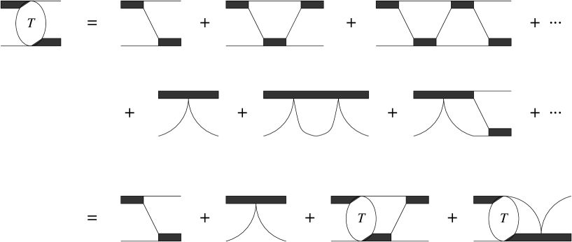
FIG. 4.: The amplitude $T$ for particle/bound-state scattering as a sum of dressed pinball and three-body-force diagrams (first and second lines) and as an integral equation (third line).

After performing the $q_{0}$ integration we can set $\epsilon=k^{2}/2m-p^{2}/2m$ and, defining $t(\vec{k},\vec{p})\equiv t(\vec{k},\vec{p},k^{2}/2m-p^{2}/2m)$, we have

$$t(\vec{k},\vec{p}) = \frac{2mg^{2}}{\frac{k^{2}}{4}+p^{2}+mB_{2}+\vec{p}\cdot\vec{k}}+h$$ (9)

$$+8\pi\lambda\int\!\frac{d^{3}q}{(2\pi)^{3}}\frac{t(\vec{k},\vec{q})}{-\frac{1}{a_{2}}+\sqrt{\frac{3q^{2}}{4}-mE}}\left[\frac{1}{-\frac{3k^{2}}{4}+mB_{2}+q^{2}+p^{2}+\vec{p}\cdot\vec{q}}+\frac{h}{2mg^{2}}\right].$$

Projection on the $S$-wave is obtained by integration over the angle between $\vec{p}$ and $\vec{k}$, resulting in

$$t(k,p) = \frac{mg^{2}}{pk}\ln\left(\frac{p^{2}+pk+k^{2}-mE}{p^{2}-pk+k^{2}-mE}\right)+h$$ (11)

$$+\frac{2\lambda}{\pi}\int_{0}^{\Lambda}dq\frac{t(k,q)q^{2}}{-\frac{1}{a_{2}}+\sqrt{\frac{3q^{2}}{4}-mE}}\left[\frac{1}{pq}\ln\left(\frac{p^{2}+pq+q^{2}-mE}{p^{2}-pq+q^{2}-mE}\right)+\frac{h}{mg^{2}}\right].$$

The scattering amplitude $T(k)$ is given by

$$T(k)=\sqrt{Z}t(k,k)\sqrt{Z},$$ (12)

where $Z$ is given by

$$Z^{-1}=i\left.\frac{\partial}{\partial p_{0}}(i\Delta(P))^{-1}\right|_{p_{0}=-B_{2}}=\frac{m^{2}g^{2}}{8\pi\sqrt{mB_{2}}}.$$ (13)

It is customary to define the function $a(k,p)$,

$$\frac{a(k,p)}{p^{2}-k^{2}}=\frac{ma_{2}}{8\pi}\frac{Zt(k,p)}{-\frac{1}{a_{2}}+\sqrt{\frac{3p^{2}}{4}-mE}},$$ (14)

that on shell reduces to

$$a(k,k)=\frac{m}{3\pi}T(k).$$ (15)

In particular, $a(0,0)=-a_{3}$. The equation satisfied by $a(k,p)$ is

$$a(k,p)=M(k,p;k)+\frac{2\lambda}{\pi}\int_{0}^{\Lambda}dq\ M(q,p;k)\frac{q^{2}}{q^{2}-k^{2}-i\epsilon}a(k,q),$$ (16)

with the kernel

$$M(q,p;k)=\frac{4}{3}\left(\frac{1}{a_{2}}+\sqrt{\frac{3p^{2}}{4}-mE}\right)\left[\frac{1}{pq}{\rm ln}\left(\frac{q^{2}+qp+p^{2}-mE}{q^{2}-qp+p^{2}-mE}\right)+\frac{h}{mg^{2}}\right].$$ (17)

Eqs. (16) and (17) reduce to the expressions found in Refs. [18, 10, 11, 12] when $h=0$. Note that the perturbative series shown in Fig. 4 corresponds to a perturbative solution of the integral equation for small $\lambda$.

The solution of Eq. (16) is complex even below the threshold for the breakup of the two-particle bound state due to the $i\epsilon$ prescription. To facilitate our discussion we will use below the function $K(k,p)$ that satisfies the same Eq. (16) as $a(k,p)$ but with the $i\epsilon$ substituted by a principal value prescription. $K(k,p)$ is real below the breakup threshold. $a(k,k)$ and, consequently, the scattering matrix can be obtained from $K(k,p)$ through

$$a(k,k)=\frac{K(k,k)}{1-ikK(k,k)}.$$ (18)

III The Problem

In order to understand the ultraviolet behavior of the theory, let us first take $h=0$. When $p\gg 1/a_{2}$ (but $k\sim 1/a_{2}$), the inhomogeneous term is small ($O(1/pa_{2})$), the main contribution to the integral comes from the region $q\sim p$, and the amplitude satisfies the approximate equation

$$K(k,p)=\frac{4\lambda}{\sqrt{3}\pi}\int_{0}^{\Lambda}\>\frac{dq}{q}\ {\rm ln}\left(\frac{q^{2}+pq+p^{2}}{q^{2}-pq+p^{2}}\right)K(k,q).$$ (19)

Now, in the limit $\Lambda\rightarrow\infty$ there is no scale left. Scale invariance suggests solutions of the form $K(k,p)=p^{s}$, which exist only if $s$ satisfies

$$1-\frac{8\lambda}{\sqrt{3}s}\frac{\sin\frac{\pi s}{6}}{\cos\frac{\pi s}{2}}=0.$$ (20)

If $K(k,p)$ is a solution, $K(k,p_{\star}^{2}/p)$ is also a solution for arbitrary $p_{\star}$. Because of this additional symmetry, the solutions of Eq. (20) come in pairs.

For $\lambda<\lambda_{c}={3\sqrt{3}\over 4\pi}\simeq 0.4135$, Eq. (20) has only real roots. For example, if $\lambda=-1/2$, there are solutions $s=\pm 2,\pm 2.17,\ldots$ In this case an acceptable solution of Eq. (19) decreases in the ultraviolet, $K(k,p\gg 1/a_{2})=Cp^{-|s|}$. For finite cutoff, the solution should still have this form as long as $p\ll\Lambda$. The overall constant $C=C(\Lambda)$ cannot be fixed from the homogeneous asymptotic equation, but is determined by matching the asymptotic solution onto the solution at $p\sim 1/a_{2}$ of the full Eq. (16). Because of the fast ultraviolet convergence, the full solution to Eq. (16) is expected to be insensitive to the choice of regulator, so that a well-defined $\lim_{\Lambda\rightarrow\infty}C(\Lambda)$ can be found. This behavior can indeed be seen in a numerical solution of Eq. (16) [11, 12].

For $\lambda=1$, on the other hand, there are purely imaginary solutions: $s=\pm is_{0}$, where $s_{0}\simeq 1.0064$. The solution of Eq. (19) as $\Lambda\rightarrow\infty$ is

$$K(k,p\gg 1/a_{2})=C\>\cos\left(s_{0}{\rm ln}\frac{p}{p_{\star}}\right).$$ (21)

Again, for finite cutoff this should hold at least for $p\ll\Lambda$, with $p_{\star}=p_{\star}(\Lambda)$ determined by the cutoff. On dimensional grounds,

$$p_{\star}(\Lambda)=\exp(-\delta/s_{0})\>\Lambda,$$ (22)

where $\delta$ is a dimensionless, cutoff independent number.

There are now two constants $C(\Lambda)$ and $\delta$: the solution of Eq. (16) is not unique in the limit $\Lambda\rightarrow\infty$ [19]. The undetermined phase $p_{\star}$ arises from the symmetry $K(k,p)\rightarrow K(k,p_{\star}^{2}/p)$. When $\lambda=-1/2$ we can dismiss the solution that grows in the ultraviolet since the integral in the Eq. (16) will not converge, but in the $\lambda=1$ case there is no way to select a preferred oscillatory solution. The same problem exists for any $\lambda$ that yields purely imaginary solutions for $s$ in Eq. (20). From now on, for definiteness we specialize to the case of purely imaginary $s$.

Solutions $K(0,p)$ of Eq. (16) for $\lambda=1$ and finite $\Lambda$ (but $h=0$) are shown in Fig. 5. We have verified that in the region $1/a_{2}\ll p\ll\Lambda$ the solutions indeed have the form (21), with $s_{0}=1.02\pm 0.01$. The phase $p_{\star}$ was found approximately linear in the cutoff in accordance with Eq. (22): $\delta=0.76\pm 0.01$ is cutoff independent. We have also found that the amplitude is

$$C=-\frac{\gamma}{\cos\left(s_{0}\ln(p_{\star}a_{2})+\epsilon\right)}$$ (23)

with $\gamma=1.50\pm 0.03$ and $\epsilon\sim 0.08$, both cutoff independent. This generates the striking meeting points at $p_{n}=a_{2}^{-1}\exp([(n+1)\pi-\epsilon]/s_{0})\sim 0.92a_{2}^{-1}(22.7)^{(n+1)}$, $n$ an integer, that can be seen in Fig. 5.

FIG. 5.: Amplitude $K(0,p)$ as function of the momentum $p$. Full, dashed, and dash-dotted curves are for $H=0$ and $\Lambda=1.0,\,2.0,\,3.0\times 10^{4}a_{2}^{-1}$, respectively. Dotted, short-dash-dotted, and short-dashed curves are for $\Lambda=1.0\times 10^{4}a_{2}^{-1}$ and $H=-6.0,\,-2.5,\,-1.8$, respectively.

Apart from these meeting points, the amplitude does not show signs of converging as $\Lambda\rightarrow\infty$. We are forced to conclude that terms that are $O(Q/\Lambda)$ cannot be dropped, as it is usually done in calculations in finite orders in perturbation theory. The presence of these terms determines a unique phase in the asymptotic region. The solution for small $p$ is to be matched at an intermediate scale to the large-$p$ solution, so the cutoff dependence leaks into the small-$p$ region. Small differences in the asymptotic phase lead to large differences in, for example, the particle/bound-state scattering length.

Since $K(k,p\gg 1/a_{2})$ is given by Eqs. (21)–(23), it is the same within a discrete family of cutoffs $\Lambda_{n}=\Lambda_{0}\exp(n\pi/s_{0})\simeq\Lambda_{0}(22.7)^{n}$, $n$ an integer. We expect that the low-energy solution will then be invariant for cutoffs in this family. If $\Lambda_{0}$ is fixed in such a way that the three-body scattering length $a_{3}$ is reproduced, then the same $a_{3}$ should result from any of the $\Lambda_{n}$’s in the same family. Moreover, the amplitude $K(k,p)$ around $p=k=0$ should be similar as well. This is indeed what we find: in Fig. 6, we plot the low-energy solutions for cutoffs in the family of $\Lambda_{0}=5.72a_{2}^{-1}$ ($\Lambda_{1}=122.2a_{2}^{-1}\simeq 22.7\Lambda_{0}$, etc.) fitted to give $a_{3}=-2.0a_{2}$ (cf. Fig. 9). For the appropriate $a_{3}/a_{2}$, we find the same cutoffs as in Ref. [20]. This generalizes the results of Ref. [20]: we see that a family of cutoffs determines not only the scattering length but also the (low-)energy dependence of the amplitude. As we vary families (i.e., $\Lambda_{0}$), however, the low-energy behavior of the amplitude shows strong cutoff dependence. This leakage of high-momentum behavior into the low-momentum physics is indication that we are not performing renormalization consistently with our expansion.

FIG. 6.: Amplitude $K(0,p)$ for $\Lambda_{0,1,2,3}$, in the family of $\Lambda_{0}=5.72a_{2}^{-1}$, corresponding to $H(\Lambda_{n})=0$, for $a_{3}=-2.0a_{2}$.

Note that if one were to truncate the series of diagrams in Fig. 4 at some finite number of loops one would miss the asymptotic behavior of $K(k,p)$ that generates this cutoff dependence. This is because $s_{0}$ (and its expansion in powers of $\lambda$) vanish in a neighborhood of $\lambda=0$. The truncation of the series in Fig. 4 is equivalent to perturbation theory in $\lambda$, and cannot produce a non-vanishing $s_{0}$. We are here facing truly non-perturbative aspects of renormalization.

IV The Solution

Faced with such a problem, the only way to eliminate this cutoff dependence is to modify our leading order calculation, that is, to change our accounting of the higher-energy behavior of the theory through the addition of at least one new interaction.

In order to do so, we can follow essentially two routes. One is to revise our systematic expansion in the two-body system. The task in this case is to enlarge the EFT in order to incorporate higher-energy degrees of freedom that have so far been treated only in something akin to a multipole expansion. Generically, the next mass scale above $1/a_{2}$ is $1/r_{2}$, and incorporating momenta $Q\sim 1/r_{2}$ means that amplitudes certainly can no longer be treated in a $Qr_{2}$ expansion. With these new elements, a new small parameter has to be identified. The resulting, new leading-order two-body amplitude might very well exhibit sufficiently nice ultraviolet behavior to guarantee the disappearance of the pronounced cutoff dependence found above in the three-body amplitudes.

While this is a perfectly legitimate way to proceed, it is in most cases not a simple task. It demands a qualitative new understanding of the shorter-range dynamics of the system under study. It is also specific to that system since the dynamics at $Q\sim 1/r_{2}$ will have to be treated in more detail; its consequences will not be common to all systems with a large $a_{2}$. Moreover, the modifications of the leading-order two-body amplitude, if any, might not resolve the leakage problem in the three-body system. We follow here the other possible route. By construction, this approach preserves the expansion of the two-body amplitude; as such it is simple, model independent, and designed to function.

The observed cutoff dependence comes from the behavior of the amplitude in the ultraviolet region, where the EFT Lagrangian, Eq. (2), is not to be trusted. When the low-energy expansion is perturbative the cutoff-dependent contribution from high loop momenta can be expanded in powers of the low external momenta and cancelled by terms in the Lagrangian, since those also give contributions analytic in the external momenta. Thus all uncertainty coming from the high momentum behavior of the theory is parametrized by the coefficients of a few local counterterms. The present case is complicated by the fact that the cutoff dependence of the amplitude is non-analytic around $p=0$. This, however, does not mean that the renormalization program in this low-energy EFT is doomed: a three-body force term of sufficient strength contributes not only at tree level, but also in loops dressed by any number of two-particle interactions. We want to show that the bare three-body force coefficient $h(\Lambda)$ can be combined with the the problematic parameter $p_{\star}(\Lambda)$ in order to produce an amplitude $K(k,p)$ which is cutoff independent, at least around $p=k=0$. Because the cutoff dependence generated by the two-body amplitude is a somewhat complicated oscillation, we expect a similar behavior of the $h(\Lambda)$ that ensures cutoff independence. In particular, $h(\Lambda)$ must be such that it vanishes for “critical” cutoffs $\Lambda_{n}$ that belong to the family that gives the desired $a_{3}$. For any other cutoff, $h(\Lambda)$ must be non-vanishing.

So, let us now consider the effects of a non-zero $h(\Lambda)$. It is convenient to rewrite the three-body force as $h(\Lambda)=2mg^{2}H(\Lambda)/\Lambda^{2}$. In the remainder of this paper we will refer to $H(\Lambda)$ as the bare three-body force. $H(\Lambda)$ has to be at least big enough so as to give a non-negligible contribution in the $p\sim k\sim\Lambda$ region. This means that the dimensionless quantity $H(\Lambda)$ has to be at least of $O(1)$. We will look for a solution initially assuming a “minimal” ansatz $H(\Lambda)\sim 1$; we subsequently show via an unbiased numerical analysis that this assumption is justified.

Such a three-body force has the feature that its contribution to the inhomogeneous term is small compared to the contribution from the two-body interaction, as it is at most $p/\Lambda$ of the latter. When $p\gg 1/a_{2}$ (but $k\sim 1/a_{2}$), the amplitude satisfies a new approximate equation

$$K(k,p)=\frac{4\lambda}{\sqrt{3}\pi}\int_{0}^{\Lambda}\>\frac{dq}{q}\ \left[{\rm ln}\left(\frac{q^{2}+pq+p^{2}}{q^{2}-pq+p^{2}}\right)+2H(\Lambda)\frac{pq}{\Lambda^{2}}\right]K(k,q).$$ (24)

For $p\sim\Lambda$ the term proportional to $H(\Lambda)$ becomes important and the solution $K(k,p\sim\Lambda)$ has a complicated form. In the range $1/a_{2}\ll p\ll\Lambda$, on the other hand, the three-body force term is suppressed by $p/\Lambda$ compared to the logarithm and can be disregarded. Consequently, the behavior (21) is still correct in the intermediate region. The effect of a finite value of $H$ can be at most to change the values of the amplitude $C$ and the phase $\delta$, which become dependent on $H$. As shown in Fig. 5, this feature is confirmed by numerical solutions: while different values of the three-body force $H$ (at a fixed $\Lambda$) preserve the form of the solution, the phase (and amplitude) are changed. If $H$ is chosen to be a function of $\Lambda$ in such a way as to cancel the explicit $\Lambda$ dependence, we can make the solution of Eq. (16) cutoff independent for all $p\ll\Lambda$. In particular, the scattering amplitude that is determined by the on-shell value $K(k,k)$ with $k\sim 1/a_{2}$ will be cutoff independent as well. For this to be possible $C$ and $\delta$ must depend on the same combination of $\Lambda$ and $H$. Thus $H(\Lambda)$ must be chosen such that

$$-s_{0}\ln\Lambda+\delta(H(\Lambda))\equiv-s_{0}\ln\Lambda_{\star},$$ (25)

where $\Lambda_{\star}$ is a (cutoff independent) parameter fixed either by experiment or by matching with a microscopic model. Eq. (25) simply means that $p_{\star}(h(\Lambda),\Lambda)=\Lambda_{\star}$ is cutoff independent, and the $1/a_{2}\ll p\ll\Lambda$ solution is

$$K(k,\Lambda\gg p\gg 1/a_{2})=-\frac{\gamma}{\cos(s_{0}\ln(\Lambda_{\star}a_{2})+\epsilon)}\>\cos\left(s_{0}{\rm ln}\frac{p}{\Lambda_{\star}}\right).$$ (26)

Matching with the $p\sim 1/a_{2}$ solution should then determine the scattering length $a_{3}=a_{3}(\Lambda_{\star})$ and the low-energy dependence of the amplitude.

For $p\sim 1/a_{2}$, Eq. (16) becomes

$$\frac{3}{4}\frac{K(k,p)}{\left(\frac{1}{a_{2}}+\sqrt{\frac{3p^{2}}{4}-mE}\right)} = \frac{1}{pk}{\rm ln}\left(\frac{p^{2}+pk+k^{2}-ME}{p^{2}-pk+k^{2}-ME}\right)$$ (29)

$$+\frac{2\lambda}{\pi p}\int_{0}^{\mu}\>dq\ {\rm ln}\left(\frac{p^{2}+pq+q^{2}-ME}{p^{2}-pq+q^{2}-ME}\right)\frac{qK(k,q)}{q^{2}-k^{2}}$$

$$+\frac{4\lambda}{\pi}\int_{\mu}^{\Lambda}\>dq\left[\frac{1}{q^{2}}+\frac{H(\Lambda)}{\Lambda^{2}}\right]K(k,q),$$

where $\mu$ is an arbitrary scale such that $\mu\ll\Lambda$, and we have dropped terms which are smaller by powers of $p/\Lambda$ or $\mu/\Lambda$. We want $K(k,p\sim 1/a_{2})$ cutoff independent and determined completely by $\Lambda_{\star}$. Then all cutoff dependence contained in the $\mu$-to-$\Lambda$ integral —in the integration limit, implicit in $K(k,p\gg 1/a_{2})$, and in $H(\Lambda)$— has to combine to produce a $\Lambda$-independent result. Achieving this means that $K(k,p\sim 1/a_{2})$ will depend only on $\Lambda_{\star}$ not just at $p=0$ but also for a range of $p$’s, because the high-momentum contributions from particle exchange and from the three-body force have the same momentum dependence. The high-momentum modes in Fig. 7(a) can be absorbed in Fig. 7(b).

FIG. 7.: Inhomogeneous terms of the integral equation (16): (a) two-body and (b) three-body kernels.

We can now obtain an approximate expression for $H(\Lambda)$. For this purpose, let us consider Eq. (29) for two different values of the cutoff $\Lambda$ and $\Lambda^{\prime}>\Lambda$, whose solutions we denote by $K(k,p)$ and $K^{\prime}(k,p)$, respectively. The equation for $K^{\prime}(k,p)$ will have the same form as the one for $K(k,p)$ except for some extra terms:

$$\frac{4\lambda}{\pi}\left\{\int_{\Lambda}^{\Lambda^{\prime}}dq\left[\frac{1}{q^{2}}+\frac{H(\Lambda)}{\Lambda^{2}}\right]K^{\prime}(k,q)+\left(\frac{H(\Lambda^{\prime})}{\Lambda^{\prime 2}}-\frac{H(\Lambda)}{\Lambda^{2}}\right)\int_{\mu}^{\Lambda}dq\>K^{\prime}(k,q)\right\}.$$ (30)

Assuming that $K^{\prime}(k,p)$ has the same phase $\cos(s_{0}\ln(p/\Lambda_{\star}))$ as $K(k,p)$ even for $p\sim\Lambda^{\prime}$, Eq. (30) becomes

$$\frac{4\lambda}{\pi\sqrt{1+s_{0}^{2}}} \left\{\right.\frac{1}{\Lambda^{\prime}}\left[\sin(s_{0}\ln({\Lambda^{\prime}}/{\Lambda_{\star}})-{\rm arctg}(1/s_{0}))+H(\Lambda^{\prime})\sin(s_{0}\ln({\Lambda^{\prime}}/{\Lambda_{\star}})+{\rm arctg}(1/s_{0}))\right]$$ (32)

$$\left.\>-(\Lambda^{\prime}\rightarrow\Lambda)\right\},$$

plus terms terms that are smaller by $\mu/\Lambda$. We can make the terms in (32) vanish if

$$H(\Lambda)=-\frac{\sin(s_{0}\ln(\frac{\Lambda}{\Lambda_{\star}})-{\rm arctg}(\frac{1}{s_{0}}))}{\sin(s_{0}\ln(\frac{\Lambda}{\Lambda_{\star}})+{\rm arctg}(\frac{1}{s_{0}}))}.$$ (33)

Note that $H(\Lambda)$ is periodic in $\Lambda$: $H(\Lambda_{n})=H(\Lambda)$ for $\Lambda_{n}=\Lambda\exp(n\pi/s_{0})\simeq\Lambda(22.7)^{n}$, $n$ an integer. In particular, the three-body force (33) vanishes at the critical cutoffs $\Lambda_{n}=\Lambda_{0}\exp(n\pi/s_{0})$ with $\Lambda_{0}=\Lambda_{\star}\exp(\arctan(1/s_{0}))$, as anticipated. Clearly, $H$ is periodic in $\Lambda_{\star}$ as well.

Since with such $H(\Lambda)$ the inhomogeneous equation for $K^{\prime}(k,p)$ is nearly the same as the equation for $K(k,p)$, it follows that $K^{\prime}(k,p)$ has also the same amplitude as $K(k,p)$ in the intermediate region. That is, $H(\Lambda)$ chosen like Eq. (33) exactly compensates any change in cutoff, so that $K^{\prime}(k,p)=K(k,p)$ for all values $p\ll\Lambda$ (up to terms suppressed by $p/\Lambda$). As a consequence, the on-shell $K$-matrix $K(k,k)$ will be $\Lambda$ independent as long as $k\ll\Lambda$.

In order to check these arguments we have numerically solved Eq. (16) for the amplitude $K(k,p)$ with a nonvanishing $H(\Lambda)$, in the case $\lambda=1$. We have fixed the scattering length $a_{3}=-K(0,0)$, and for several cutoffs we have determined the three-body force that is necessary to keep $a_{3}$ unchanged. With such a procedure, we have obtained $H(\Lambda)$ for different $\Lambda$’s. In Fig. 8 we plot the corresponding numerical values for the case $a_{3}=1.56a_{2}$, together with our approximate analytical expression (33) with $\Lambda_{\star}=19.5a_{2}^{-1}$. The remarkable agreement confirms that the solution for $H(\Lambda)$ is very close to the minimal one, all the way up to very high values of $\Lambda$. Note that the three-body force vanishes at the critical cutoffs in the family generated by $\Lambda_{0}=\Lambda_{\star}\exp(\arctan(1/s_{0}))=42.6a_{2}^{-1}$.

FIG. 8.: Three-body force $H$ as a function of the cutoff $\Lambda$ for $a_{3}=1.56a_{2}$: numerical solution (dots) and Eq.(33) with $\Lambda_{\star}=19.5a_{2}^{-1}$ (solid line).

In Fig. 9 we show results for the corresponding $K(k,k)^{-1}=k\cot\delta$, where $\delta$ is the $S$-wave phase shift for particle/bound-state scattering, for different cutoffs in the case $a_{3}=1.56a_{2}$. Comparison with Fig. 5 shows that by introduction of the three-body force we have succeeded in removing the cutoff dependence of the low-$k$ region, thus generalizing Fig. 6 to cutoffs other than critical. As argued above, $k\cot\delta$ is insensitive to $\Lambda$ as long as $k\ll\Lambda$. The effective range, for example, is predicted as $r_{3}=0.57a_{2}$. In Fig. 10 we plot the $S$-wave phase shifts directly.

FIG. 9.: Energy dependence for $\Lambda_{\star}=19.5a_{2}^{-1}$: $k\cot\delta$ as function of $k$ for different cutoffs ($\Lambda=42.6,\,100.0,\,230.0,\,959.0\times a_{2}^{-1}$).

FIG. 10.: $S$-wave phase shifts $\delta$ as function of energy $E$, as predicted by the EFT when $a_{3}=1.56a_{2}$ ($\Lambda=42.6,\,100.0,\,230.0,\,959.0\times a_{2}^{-1}$).

Similar results can be obtained for other values of $a_{3}$. By repeating this procedure we can in fact obtain $a_{3}=a_{3}(\Lambda_{\star})$ or vice-versa. This is shown in Fig. 11. The periodicity of the three-body force with $\Lambda_{\star}$ is apparent. If the underlying theory is known and can be solved, then $\Lambda_{\star}$ can be determined in terms of underlying parameters, and $a_{3}$ can also be predicted. Otherwise, we can use $a_{3}$ or any other low-energy three-body datum to determine $\Lambda_{\star}$ empirically. In either case, once the two-body scattering length $a_{2}$ is fixed, the low-energy particle/bound-state scattering amplitude is completely determined by the mass scale $\Lambda_{\star}$ contained in the three-body force $h$.

FIG. 11.: Particle/bound-state scattering length $a_{3}$ as function of the three-body force parameter $\Lambda_{\star}$.

V Bound State

We can extend the preceding analysis to the three-body bound-state problem. In this case the relevant equation to be solved is Eq. (16) without inhomogeneous terms. The latter did not play an important role in our ultraviolet arguments, so the same arguments hold for any bound state with binding energy $B_{3}$ comparable with $1/ma_{2}^{2}$, i.e., for any bound state with the dimensionless binding energy $b_{3}=ma_{2}^{2}B_{3}=O(1)$. Such bound states are shallow, having a size $\sim 1/\sqrt{mB_{3}}=a_{2}/\sqrt{b_{3}}$ comparable to $a_{2}$, and thus should be within range of the EFT. In principle, all bound states with size larger than $\sim r_{2}$ should be amenable to this EFT description. Their properties will be determined in first approximation by only $a_{2}$ and $a_{3}$, or equivalently $C_{0}$ and $\Lambda_{\star}$, while more precise information can be obtained in an expansion in $\sqrt{b_{3}}r_{2}/a_{2}$.

In Fig. 12 we plot binding energies for a range of cutoffs, with the three-body force adjusted to give a fixed scattering length $a_{3}=1.56a_{2}$. (With an appropriate $a_{3}$, our results reduce to those of Ref. [20] when the cutoff is at one of the critical values $\Lambda_{n}$.) As we can see, for this value of $\Lambda_{\star}$ there exists a shallow bound state at $b_{3}\simeq 2$ whose binding energy is independent of the cutoff. This bound state has a size $\sim 0.7a_{2}$ and can thus be studied within the EFT. As we increase the cutoff, deeper bound states appear at $\Lambda_{n}=\Lambda_{0}\exp(n\pi/s_{0})$ with $n$ an integer and $\Lambda_{0}\simeq 10$, so that for $\Lambda_{n-1}\leq\Lambda\leq\Lambda_{n}$ there are $n+1$ bound states. The next-to-shallowest bound state has $b_{3}\simeq 70$ and thus a size $\sim 0.1a_{2}$. If the underlying theory is such that $r_{2}$ $\stackrel{{\scriptstyle\textstyle<}}{{\sim}}$ $a_{2}/10$, a cutoff $\Lambda$ $\stackrel{{\scriptstyle\textstyle>}}{{\sim}}$ $1/r_{2}$ allows us to deal with the next-to-shallowest bound state. The next deeper bound state has $b_{3}\simeq 4\times 10^{4}$ and thus a size $\sim 0.01a_{2}$, and so on. These most likely lie outside the EFT.

FIG. 12.: Three-body binding energies $B_{3}$ as functions of the cutoff $\Lambda$ for $\Lambda_{\star}=19.5a_{2}^{-1}$.

Properties of the shallowest bound state, if within the EFT, are model independent and thus the most interesting. For a fixed $a_{2}$, they are determined by $\Lambda_{\star}$. In Fig. 13 we plot the binding energy $B_{3}$ as function of $\Lambda_{\star}$. This should be compared with the behavior of $a_{3}=a_{3}(\Lambda_{\star})$ shown in Fig. 11. It is clear that at $\Lambda_{\star}\sim 4a_{2}^{-1}$ a bound state appears at zero energy. As $\Lambda_{\star}$ increases, this state gets progressively more bound until at $\Lambda_{\star}\sim 22.7\times 4a_{2}^{-1}$ a new shallowest bound state appears; the picture repeats indefinitely. Whenever a bound state is close to zero energy, $a_{3}$ is large in magnitude, negative if the bound state is virtual and positive if real. This can be seen in Fig. 11.

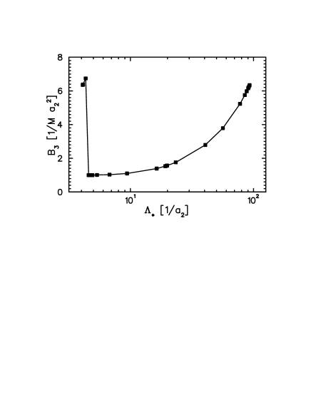
FIG. 13.: Binding energy $B_{3}$ of the shallowest bound state as function of the parameter $\Lambda_{\star}$.

Eliminating $\Lambda_{\star}$, we obtain an universal curve $B_{3}=B_{3}(a_{3})$, as in Fig. 14. Qualitative features of this curve can be understood from Figs. 11 and 13. For $a_{3}$ large in magnitude, small variations of $\Lambda_{\star}$ lead to large variations of $a_{3}$ but small variations of $B_{3}$, so the curve flattens out at both ends. For $a_{3}$ large and positive, there is a shallow real bound state; for $a_{3}$ large and negative, there is a shallow virtual bound state but the curve tracks the deeper real bound state. For $a_{3}\sim a_{2}$, $a_{3}$ and $B_{3}$ vary with $\Lambda_{\star}$ at a similar rate, and the curve interpolates between the two ends.

This curve is known in the three-nucleon case as the Phillips line [3]. It has been derived before in the context of models for the two-particle potential that differed in their high-momentum behavior. Varying among two-particle potential models one could expect to fill up the $B_{3}\times a_{3}$ plane. In the EFT, the high-momentum behavior of the two-particle potential is butchered, which causes no trouble in describing two-particle scattering at low-energies, but —in the peculiar way described here— does require a three-body force. It is crucial that the EFT does retain a systematic expansion, so that in leading order it requires only one local three-body counterterm, determined by $\Lambda_{\star}$. Varying among two-particle potential models is thus equivalent to varying the one parameter $\Lambda_{\star}$ of the three-body force. This spans a single curve $B_{3}=B_{3}(a_{3})$ in the $B_{3}\times a_{3}$ plane. Our argument suggests that the Phillips line is a generic phenomenon and provides a simple explanation of its origin.

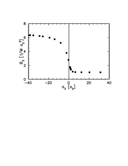
FIG. 14.: Phillips line: binding energy $B_{3}$ of the shallowest bound state as function of the particle/bound-state scattering length $a_{3}$.

VI Higher orders

The corrections to the calculations in the previous sections come from operators not explicitly written in Eq. (1) and are suppressed by powers of $kR$ or $R/a_{2}$. The first correction comes from terms involving two derivatives and four nucleons fields [6]:

$$-\frac{C_{2}}{8}(\psi^{\dagger}\psi\,\psi^{\dagger}\nabla^{2}\psi+\ldots).$$ (34)

They account for the effective range term in the effective range expansion of particle-particle scattering, and one finds $C_{2}=\pi a_{2}^{2}r_{2}/m$. As it was done before, (34) can also be generated by integrating out the $T$ field from Eq. (2) if the extra term

$$g_{2}T^{\dagger}(i\partial_{0}+\frac{\nabla^{2}}{4m})T,$$ (35)

where $g_{2}/\Delta=4mC_{2}/C_{0}$, is added to Eq. (2). Indeed, integration over the auxiliary field $T$ generates, besides the terms shown in Eq. (1), also a four-nucleon term involving two space derivatives or one time derivative. As usual, a nucleon-field redefinition involving the equations of motion can be performed to trade the time derivative by two space derivatives. This field redefinition does not change on-shell amplitudes. As far as observables are concerned, adding (35) to Eq. (2) is thus equivalent to adding (34) to Eq. (1).

The correction proportional to $r_{2}$ is then given by the diagram in Fig. 15(a) (plus corresponding wave function renormalization pieces) and includes one insertion of the kinetic term, Eq. (35). The contribution of this graph to $t(k,p)$ is

$$\frac{g_{2}}{2\pi^{2}}\int_{0}^{\infty}\!dq\,q^{2}\,it(q,p)\,(i\Delta(3k^{2}/4m-1/ma_{2}^{2}-q^{2}/2m,\vec{q}))^{2}\left(\frac{3(k^{2}-q^{2})}{4m}-\frac{1}{ma_{2}^{2}}\right)it(k,q).$$ (36)

As discussed above, $t(k,p)$ behaves for large $p$ as $t(k,p)\sim A(k)\cos(s_{0}\log(p/\Lambda_{\star}))/p$, so the diagram is naively linearly divergent. The identity

$$\frac{1}{a_{2}}\frac{q^{2}-k^{2}}{(-\frac{1}{a_{2}}+\sqrt{\frac{3(q^{2}-k^{2})}{4}+\frac{1}{a_{2}^{2}}})^{2}}=\frac{4}{3}\left[1+\frac{\frac{2}{a_{2}}(\sqrt{\frac{3(q^{2}-k^{2})}{4}+\frac{1}{a_{2}^{2}}}-\frac{1}{a_{2}})}{\frac{3(q^{2}-k^{2})}{4}-\frac{2}{a_{2}}(\sqrt{\frac{3(q^{2}-k^{2})}{4}+\frac{1}{a_{2}^{2}}}-\frac{1}{a_{2}})}\right]$$ (37)

can be used to rewrite Eq. (36) and it shows that the most divergent piece (the one due to the constant on the right hand side of Eq. (37)) actually vanishes. This is because in this term the integral can be closed in the complex plane without circling any pole. The only contribution comes from the second term in Eq. (37) but this term is further suppressed in the ultraviolet, resulting in a logarithmically divergent contribution from the diagram in Fig. 15(a). This divergent piece has a complicated dependence on the external momentum $k$ since it is proportional to $A^{2}(k)$ (the dependence on $k$ of the other terms included in the graph is unimportant in the ultraviolet). This is an unusual situation. In perturbative calculations the divergent part is simply a polynomial in the external momenta and it can consequently be absorbed in a finite number of local counterterms appearing only at tree level. Here the dependence on the external momenta is more complicated but the counterterm appears in graphs with an arbitrary number of leading-order interactions. To see this, let us split the three-body force coefficient $h$ into a leading order piece $h^{(0)}$ (the same considered in the previous sections) and a sub-leading piece $h^{(1)}$ that will be included perturbatively. The inclusion of the sub-leading three-body force proportional to $h^{(1)}$ generates the three diagrams shown in Fig. 15(b,c,d). Simple power counting shows that the graph in Fig. 15(d) is the most divergent of the three. The important point is that the external momentum dependence of the most divergent part of the graph in Fig. 15(d) is given by $A^{2}(k)$, again because the dependence on the external momentum $k$ of the nucleon propagators in Fig. 15(d) can be discarded in the ultraviolet region. Since the $k$ dependence of the divergent part is the same in Fig. 15(a) and Fig. 15(d), $h^{(1)}$ can be chosen as a function of the cutoff so as to make the sum of these two graphs finite. As always, the renormalization procedure leaves a finite piece in $h$ undetermined that should be fixed through the use of one experimental input. This conclusion seems to agree with Ref. [21]. More details of the calculation of the range correction as applied to the case of three nucleons in the triton channel are left for a future publication.

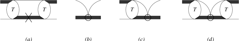
FIG. 15.: $O(r_{2}/a_{2})$ diagrams: (a) one insertion of (35) in the dimeron propagator, denoted by a cross; (b,c,d) one insertion of a correction to the three-body force $h$, denoted by a circle.

VII Discussion and Conclusion

Our results should hold for ⁴He atoms. In fact, it has recently been established that the two-⁴He bound state (“dimer”) is very shallow, with an average size $\langle r\rangle=62\pm 10$ Å [22], more than an order of magnitude larger than the range of the interatomic potential. The low-energy two-⁴He system should then be describable by contact two-body forces. In leading order, the measured size translates into a scattering length $a_{2}=124$ Å, which determines the strength of the contact interaction. Unfortunately, although the three-⁴He (“trimer”) has been observed [23], there seems to be no low-energy information on its properties nor on ⁴He/dimer scattering. At least one three-body datum is needed to determine $\Lambda_{\star}$ and use the EFT to make predictions.

Until such datum becomes available, we can only illustrate the method by using a phenomenological ⁴He-⁴He potential as a model of a microscopic theory. We select a potential [24] which is consistent with the recent measurement of the dimer binding energy. It gives for the two-body system $a_{2}=124.7$ Å and $r_{2}\simeq 7.4$ Å. Three-body calculations are much more difficult to perform with such a phenomenological potential. An estimate for the ⁴He/dimer scattering length is $a_{3}=195$ Å. Ground and excited bound states have been reported; estimates for the shallowest bound state place it in the range $B_{3}=1.04-1.7$ mK, while a deeper state lies around $B_{3}=0.082-0.1173$ K. There exist a prediction for the low-energy $S$-wave phase shifts, albeit for a different potential, but $r_{3}$ could not be determined.

Using such model we can estimate the range of validity of the EFT in momentum to be $\sim 1/r_{2}\simeq 0.14$ Å^-1, and the leading order to give an accuracy of $\sim r_{2}/a_{2}\simeq 0.06$, or about 10%, at momenta $Q\sim 1/a_{2}$. Using this potential’s $a_{3}/a_{2}=1.56$ we can determine $\Lambda_{\star}$, and predict both the energy dependence in ⁴He/dimer scattering and the trimer binding energy. In fact, in Figs. 9, 10, and 12, we have used exactly this value of $a_{3}$. As a consequence, Fig. 9 represents our lowest-order prediction for $k\cot\delta$ for atom/dimer scattering, from which we can for the first time extract an effective range $r_{3}=71$ Å. Fig. 10 displays the $S$-wave phase shifts themselves, and is in qualitative agreement with the result of Ref. [24] for a similar potential, being obtained here at a negligible fraction of computer time. From Fig. 12 we predict a bound state at $B_{3}=1.2$ mK, which is certainly within the EFT. The next-to-shallowest bound state is small enough to be at the border of EFT applicability. For a sufficiently large cutoff, we find $B_{3}=0.057$ K, but in the best case scenario corrections from higher orders should be a lot larger than 10%, and very important.

Because of the similarity of the integral equations, our arguments should be relevant for systems of three fermions with internal quantum numbers as well. We are in the process of verifying this for the three-nucleon system in the $J=1/2$ channel, where we will be able to check our predictions against the energy dependence of existing phase shift analyses of neutron-deuteron scattering and against the triton binding energy [25]. We also plan to extend our calculations to the four-and-more-body system and search for the existence of other leading few-body forces.

These results will hold in an EFT where the pion has been integrated out, which is valid for $Q$ $\stackrel{{\scriptstyle\textstyle<}}{{\sim}}$ $m_{\pi}$. In an exciting new development, it has been argued in Ref. [7] that there is a region of momenta above $m_{\pi}$ where, although pions have to be kept explicitly, their effects are sub-leading. The leading two-body operators are thus the same as in the “pionless” theory. A number of examples seem to corroborate this picture [14]. In this case, our leading-order results will be valid in this “pionful” theory as well, suggesting that our bound-state calculation will provide a reasonable estimate of the triton binding energy.

In conclusion, we have provided analytical and numerical evidence that renormalization of the three-body problem with short-range forces requires in general the presence in leading order of a one-parameter contact three-body force. This frames results obtained earlier with particular models within a larger, model-independent picture. It opens up the possibility of applying the EFT method to a large class of systems of three or more particles with short-range forces.

Acknowledgments

We thank V. Efimov, H. Müller, and D. Kaplan for helpful discussions. HWH and UvK acknowledge the hospitality of the Nuclear Theory Group and the INT in Seattle, where part of this work was carried out. This research was supported in part by the U.S. Department of Energy grants DOE-ER-40561 and DE-FG03-97ER41014, the Natural Science and Engineering Research Council of Canada, and the U.S. National Science Foundation grant PHY94-20470.

REFERENCES

- [1] L.H. Thomas, Phys. Rev. 47 (1935) 903; S.K. Adhikari, T. Frederico, and I.D. Goldman, Phys. Rev. Lett. 74 (1995) 487.
- [2] V.N. Efimov, Sov. J. Nucl. Phys. 12 (1971) 589; Phys. Rev. C47 (1993) 1876.
- [3] A.C. Phillips, Nucl. Phys. A107 (1968) 209.
- [4] G.P. Lepage, in “From Actions to Answers, TASI’89”, T. DeGrand and D. Toussaint (editors), World Scientific, 1990; D.B. Kaplan, nucl-th/9506035; H. Georgi, Ann. Rev. Part. Sci. 43 (1994) 209.
- [5] E. Braaten and A. Nieto, Phys. Rev. B56 (1997) 14745; Phys. Rev. B55 (1997) 8090.
- [6] U. van Kolck, in Proceedings of the Workshop on Chiral Dynamics 1997, Theory and Experiment, A. Bernstein, D. Drechsel, and T. Walcher (editors), Springer–Verlag, 1998, hep-ph/9711222; in Ref. [9]; nucl-th/9808007.
- [7] D.B. Kaplan, M.J. Savage, and M.B. Wise, Phys. Lett. B424 (1998) 390; nucl-th/9802075.
- [8] J. Gegelia, nucl-th/9802038; nucl-th/9805008; M.C. Birse, J.A. McGovern, and K.G. Richardson, hep-ph/9807302; hep-ph/9808398; T.D. Cohen and J.M. Hansen, nucl-th/9808006.
- [9] “Nuclear Physics with Effective Field Theory”, R. Seki, U. van Kolck, and M.J. Savage (editors), World Scientific, 1998.
- [10] P.F. Bedaque, in Ref. [9], nucl-th/9806041.
- [11] P.F. Bedaque and U. van Kolck, Phys. Lett. B428 (1998) 221.
- [12] P.F. Bedaque, H.-W. Hammer, and U. van Kolck, Phys. Rev. C58 (1998) R641.
- [13] S. Weinberg, Phys. Lett. B251 (1990) 288; Nucl. Phys. B363 (1991) 3; Phys. Lett. B295 (1992) 114; C. Ordóñez and U. van Kolck, Phys. Lett. B291 (1992) 459; C. Ordóñez, L. Ray, and U. van Kolck, Phys. Rev. Lett. 72 (1994) 1982; Phys. Rev. C53 (1996) 2086; U. van Kolck, Phys. Rev. C49 (1994) 2932; J.L. Friar, D. Hüber, and U. van Kolck, nucl-th/9809065.
- [14] D.B. Kaplan, M.J. Savage and M.B. Wise, nucl-th/9804032; J.-W. Chen et al, nucl-th/9806080; M.J. Savage and R.P. Springer, nucl-th/9807014; D.B. Kaplan et al, nucl-th/9807081; J.-W. Chen et al, nucl-th/9809023; J.-W. Chen, nucl-th/9810021.
- [15] J. Gegelia, nucl-th/9806028; T.D. Cohen and J.M. Hansen, nucl-th/9808038; T. Mehen and I.W. Stewart, nucl-th/9809071; nucl-th/9809095.
- [16] P.F. Bedaque, H.-W. Hammer, and U. van Kolck, nucl-th/9809025.
- [17] D.B. Kaplan, Nucl. Phys. B494 (1997) 471.
- [18] G.V. Skorniakov and K.A. Ter-Martirosian, Sov. Phys. JETP 4 (1957) 648.
- [19] G.S. Danilov and V.I. Lebedev, Sov. Phys. JETP 17 (1963) 1015;
- [20] V.F. Kharchenko, Sov. J. Nucl. Phys. 16 (1973) 173.
- [21] V.N. Efimov, Phys. Rev. C44 (1991) 2303.
- [22] F. Luo, C.F. Giese, and W.R. Gentry, J. Chem. Phys. 104 (1996) 1151.
- [23] W. Schöllkopf and J. Peter Toennies, J. Chem. Phys. 104 (1996) 1155.
- [24] Y.-H. Uang and W.C. Stwalley, J. Chem. Phys. 76 (1982) 5069; S. Nakaichi-Maeda and T.K. Lim, Phys. Rev. A28 (1983) 692; A.K. Motovilov, S.A. Sofianos, and E.A. Kolganova, Chem. Phys. Lett. 275 (1997) 168.
- [25] P.F. Bedaque, H.-W. Hammer, and U. van Kolck, in progress.