Abstract

High energy strong interaction physics is successfully described by the local renormalizable gauge theory called Quantum–Chromo–Dynamics (QCD) with quarks and gluons as “elementary” degrees of freedom, while intermediate energy strong interaction physics shows up to be determined by a non–local, non–renormalizable effective field theory (EFT) of “effective” degrees of freedom like mesons, ground state baryons and resonances. The connection between high and intermediate physics is established by a change of basis (“bosonisation”) from the infinite Fock–state basis of quarks and gluons to the infinite Fock–state basis of the “effective” degrees of freedom. The infinite number of counter terms in the Lagrangian of such an non–renormalizable EFT is replaced by a tree–level Lagrangian containing a finite number of interaction terms dressed by non–local vertex–functions commonly called formfactors (containing cutoffs) generating the dynamics of an infinity of interaction diagrams in an EFT. Furthermore low and intermediate energy physics successfully is described by the use of resonance propagators, i.e. resonances are treated like “degrees of freedom”, which are seen in the experiment and behave like particles with complex mass which is usually not compatible with the idea of unitarity.

In analogy to the role of vertex-functions in non–renormalizable theories and with respect to the infinite dimension of the effective Fock-state basis I present a “toy-model” in which fermionic and bosonic resonances are considered to be “particles”, i.e. they consistently are described by (anti-)commuting effective field-operators (containing dynamics of infinitely many quark-gluon or meson-nucleon diagrams) which are comfortably treated by Wick’s Theorem in a covariant framework and obey unitarity. Non–trivial implications to couplings of non–local interactions are shown.

Key-words: bosonisation, double-counting, effective degree of freedom, effective field theory, renormalization, resonance, self-energy, unitarity, unitary effective resonance model, vertex-function

1 Introduction

Why does a intermediate energy theorist hold a talk on a high energy physics and QCD conference? The answer of this question is obvious: The high and the intermediate energy approaches to strong interaction physics are treating the same problem, i.e. revealing the physical nature of the phase transition region (see Fig. 1), from two different directions. Both approaches are connected on fundamental theoretical grounds, use similar techniques and suffer more or less similar problems in the non–perturbative regime. The solution to the problem of the phase transition consists of a consistent combination of the theoretical framework of both sides forming one fundamental framework describing the theory of strong interaction. Hopeful steps in this direction based on chiral symmetry constraints and analyticity properties lead e.g. to Chiral Perturbation Theory [1, 2, 3] and the QCD Sum Rule method [4, 5, 6].

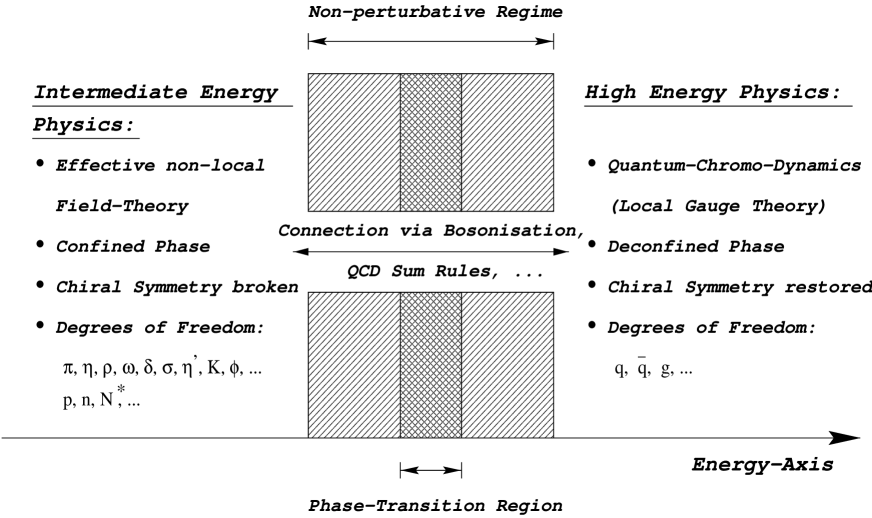
Figure 1: Confrontation of intermediate and high energy strong interaction physics.

Using the constraint of unitarity I want to study the property of self–energies and vertex–functions (“formfactors”) in nonlocal effective (bosonised) intermediate energy field theories. The reason is simple: The experimental situation in intermediate energy proton–proton and proton–nucleus colliders improved a lot. In cooled synchrotrons (e.g. at COSY, WASA, $\ldots$) the experimentalists produce high precision datas for exclusive meson production processes at threshold like $pp\rightarrow pp\,\pi^{0}$, $pp\rightarrow pp\,\eta$, $pp\rightarrow p\Lambda K$, $pp\rightarrow pp\,\phi$, $pp\rightarrow pp\,\pi\pi$, $pd\rightarrow{}^{3}H\!e\,\eta$ , $\ldots\,$. The high energy and momentum transfers involved in these reactions excite all kinds of effective degrees of freedom like hyperons, resonances, $\ldots\,$. The physics involved for heavy meson production is so short ranged that intermediate energy theorists have to leave common grounds and describe the short ranged processes by high energy approaches in the non–perturbative regime which involve quarks and gluons. The formfactors mentioned contain all kinds of thinkable short range physics which have to be revealed to get an understanding what’s going on in the non–perturbative range between intermediate and high energy physics. Furthermore the comparison of experimental datas and theoretical calculations show a high sensitivity of different isospin–channels to interference effects between various subprocesses leading to the production of the considered mesons. Interference effects are connected to the imaginary parts of production amplitudes which are due to complex self–energies of intermediate resonances, loop contributions and — as I will show — complex vertex functions at the interaction vertices. The contradictions arrising with respect to time reversal invariance and unitarity of theory can be resolved by a systematic introduction of effective degrees of freedom and the application of certain constraints to vertex–functions and self–energies due to unitarity.
As a final remark I want to mention that some of the present interests of intermediate energy theorists should be very common to high energy physicists: e.g. the question on the strangeness and spin content of the proton and its excitations, the investigation of Zweig-rule violations, the nature of non–abelian non–linear field-theories, $\ldots\,$.

2 A simple classification scheme for resonances

From Quantum Mechanics we know that close to a resonance $\cot\delta_{\ell}(E)$ is variing rapidly as a function of the energy $E$, i.e. we can expand $\cot\delta_{\ell}(E)$ at the resonance energy $E_{R}$:

$$\cot\delta_{\ell}(E)\quad=\quad\underbrace{\cot\delta_{\ell}(E_{R})}_{=0}\;+\;\frac{\partial\cot\delta_{\ell}(E)}{\partial E}\Bigg{|}_{E=E_{R}}(E-E_{R})\;+\;\ldots$$ (1)

Using this expansion it simple to see that the partial scattering aplitude $f_{\ell}(E)$ develops a Breit–Wigner shape (with a partial width $\Gamma_{\ell}$):

$$f_{\ell}(E)=\frac{1}{k(\cot\delta_{\ell}-i)}\approx-\;\frac{1}{k_{R}}\;\frac{\Gamma_{\ell}/2}{E-E_{R}+i\Gamma_{\ell}/2}\quad\mbox{with}\quad\frac{2}{\Gamma_{\ell}}:=-\frac{\partial\cot\delta_{\ell}(E)}{\partial E}\Bigg{|}_{E=E_{R}}$$ (2)

It is now important to mention that — although the T–matrix develops an imaginary part — in this class of resonances there is no inelasticity present, i.e. unitarity is still fulfilled, if the partial phaseshifts $\delta_{\ell}$ are real.
In a second class of resonances absorptivity, i.e. inelasicity is present, sometimes desired. In such a case the whole system looses probability. In the well known “Wigner–Weisskopf approximation” the decay of particles is described by a non–Hermitian Hamilton–operator. These decaying particles have (like resonances) a finite decay width $\Gamma$ which determine the non–diagonal elements of the Hamilton–operator. The reason for the inelasticity in this kind of approaches is, that parts of the Hilbert–space have been removed from the problem, i.e. the Hilbert–space/Fock–space is incomplete. Examples for this approach are the optical potential method and the description of $K^{0}$-$\bar{K}^{0}$–oszillations.

3 Self–energies and vertex–functions in renormalizable and non-renormalizable field theories

Looking at equation (2) one could assume that the self–energy or resonance width is constant. That this is not the general case can be seen from the normalizable local gauge theory QED. Here the electron propagator $G^{\bar{e}e}(-p,p)=i(\!\!\,{\not{\!p}}-m_{e}+\Sigma^{\bar{e}e}(p))^{-1}$ develops by the renormalization procedure a momentum dependent self–energy $\Sigma^{\bar{e}e}(p)$. To one loop one obtains:

$$\Sigma^{\bar{e}e}(p)=i\,e^{2}\,\int\frac{d^{4}q}{(2\pi)^{4}}\frac{\gamma_{\alpha}(\,{\not{\!q}}+m_{e})\,\gamma^{\alpha}}{(q^{2}-m^{2}_{e})((q-p)^{2}-\lambda^{2})}$$ (3)

In the same way the bare electron–photon–vertex picks up a momentum dependence, i.e. $i\,e\,\gamma^{\mu}\rightarrow i\,e\,\gamma^{\mu}+i\,e\,\Lambda^{\mu}(p^{\prime},p)$. Examples for self–energies developing momentum dependent imaginary parts are quasi–particle excitations in finite density field–theories and the famous “Landau–damping”. Of course, the contact to a heat bath or a finite medium locally violates unitarity, i.e. is inelastic. But how about resonances in effective field theories propagating in the vacuum? If resonant effective degrees of freedom are present in an effective field theory of strong interaction, the corresponding effective Lagrangian should not contain inelasticities, i.e. it should be Hermitian, as it should be derivable by an unitary transformation from the Hermiatian Lagrangian of QCD. In such a transformation the gluons have to be integrated out from the generating functional (which is not possible at present). After “Fierz-ing” properly the so obtained multi-quark-Lagrangian and introducing source-terms for mesons and baryons with all kinds of quantum numbers, the quark-fields have to be integrated out, to obtain an non–local effective action of all the mesonic and baryonic sources. Finally the infinity of interaction terms in the non-local Lagrangian obtained have to be replaced by a tree-level Lagrangian containing complex momentum dependent vertex–functions and self–energies. The following toy model will show that resonance sources have to appear pairwise due to unitarity.

4 The “Unitary Effective Resonance Model”

4.1 Field theoretic effective model for one fermionic resonance

At this point I only roughly sketch a toy model developed for the consistent description of effective resonant degrees of freedom in intermediate energy strong interaction physics. For a more complete view I refer to references [7][8].
It is very common in intermediate energy physics to describe the propagation of a fermionic resonance with the complex “mass” $M=m_{\ast}-i\,\Gamma/2$ ($m_{\ast}$ is the real part of the mass $M$, $\Gamma$ is the resonance width) by the introduction of a propagator of the form $(\!\!\,{\not{\!p}}-M)^{-1}$. That this simplistic picture is not well defined can be seen, if one “naively” tries to write down a free Lagrangian for a fermionic resonance field $\Psi(x)$ in the following way:

$${\cal L}_{0}(x)\quad\stackrel{{\scriptstyle?}}{{=}}\quad\bar{\Psi}(x)\;\bigg{(}\frac{1}{2}\;(i\!\,{\not{\!\partial}}-i\!\!\stackrel{{\scriptstyle\leftarrow}}{{\,{\not{\!\partial}}}})-m_{\ast}+\frac{i}{2}\,\Gamma\bigg{)}\;\Psi(x)\quad$$ (4)

The action $S_{0}=\int\!d^{4}x\,{\cal L}_{0}(x)$ related to this Lagrangian is not Hermitian. But Hermiticity of the action is the minimum requirement for a CPT-invariant and unitary theory describing strong interaction only. Additionally, if one tries to “quantize” such an effective resonance field, i.e. introduce field operators, anticommutation relations, $\ldots$ one immediately runs into inconsistencies. To avoid all mentioned troubles one is forced to introduce two distinct field operators $\bar{\Psi}_{L}(x)$ und $\Psi_{R}(x)$ (“left” and “right” eigen-fields) and their complex conjugates, to describe one resonance degree of freedom in an effective field theoretic way by the following free Lagrangian density:

$${\cal L}_{0}(x) = \alpha\;\bar{\Psi}_{L}(x)\;\bigg{(}\frac{1}{2}\;(i\!\,{\not{\!\partial}}-i\!\!\stackrel{{\scriptstyle\leftarrow}}{{\,{\not{\!\partial}}}})-m_{\ast}+\frac{i}{2}\,\Gamma\bigg{)}\;\Psi_{R}(x)\quad+$$

$$+ \alpha^{\ast}\;\bar{\Psi}_{R}(x)\;\bigg{(}\frac{1}{2}\;(\underbrace{i\!\,{\not{\!\partial}}-i\!\!\stackrel{{\scriptstyle\leftarrow}}{{\,{\not{\!\partial}}}}}_{\displaystyle=:i\!\!\stackrel{{\scriptstyle\;\,\leftrightarrow}}{{\,{\not{\!\partial}}}}})-m_{\ast}-\frac{i}{2}\,\underbrace{\gamma_{0}\,\Gamma^{+}\,\gamma_{0}}_{\displaystyle\stackrel{{\scriptstyle!}}{{=}}\Gamma}\bigg{)}\;\Psi_{L}(x)$$

($\alpha$ is an arbitrary complex constant chosen to be 1). The classical Euler–Lagrange equations with respect to variation of the action by $\Psi^{+}_{L}(x)$, $\Psi^{+}_{R}(x)$, $\Psi_{L}(x)$ and $\Psi_{R}(x)$ are the following generalized ”Dirac-equations”:

$$\begin{array}[]{rcr}{(i\!\,{\not{\!\partial}}-M)\;\Psi_{R}(x)\quad=\quad 0}&&{\bar{\Psi}_{R}(x)(-i\!\!\stackrel{{\scriptstyle\leftarrow}}{{\,{\not{\!\partial}}}}-M^{\ast})\quad=\quad 0}\\ {(i\!\,{\not{\!\partial}}-M^{\ast})\;\Psi_{L}(x)\quad=\quad 0}&&{\bar{\Psi}_{L}(x)(-i\!\!\stackrel{{\scriptstyle\leftarrow}}{{\,{\not{\!\partial}}}}-M)\quad=\quad 0}\end{array}$$

(5)

These classical equations of motion can be solved by a simple Laplace–transformation. The corresponding transformation for the field–operators is:

$$\Psi_{R}(x) = \sum\limits_{s}\,\int\!\!\frac{d^{3}k\;\sqrt{2M}}{\sqrt{(2\pi)^{3}\;2\omega_{R}\,(|\vec{k}\makebox[1.00006pt]{}|)}}\Big{[}u_{R}\,(\vec{k},s)\;b_{R}\,(\vec{k},s)\;e^{\displaystyle-\,ik_{R}x}+v_{R}\,(\vec{k},s)\;d^{+}_{R}\,(\vec{k},s)\;e^{\displaystyle ik_{R}x}\Big{]}$$

$$\Psi_{L}(x) = \sum\limits_{s}\,\int\!\!\frac{d^{3}k\;\sqrt{2M^{\ast}}}{\sqrt{(2\pi)^{3}\;2\omega_{L}\,(|\vec{k}\makebox[1.00006pt]{}|)}}\Big{[}u_{L}\,(\vec{k},s)\;b_{L}\,(\vec{k},s)\;e^{\displaystyle-\,ik_{L}x}+v_{L}\,(\vec{k},s)\;d^{+}_{L}\,(\vec{k},s)\;e^{\displaystyle ik_{L}x}\Big{]}$$

$$\bar{\Psi}_{R}(x) = \sum\limits_{s}\,\int\!\!\frac{d^{3}k\;\sqrt{2M^{\ast}}}{\sqrt{(2\pi)^{3}\;2\omega_{L}\,(|\vec{k}\makebox[1.00006pt]{}|)}}\Big{[}\bar{v}_{R}\,(\vec{k},s)\;d_{R}\,(\vec{k},s)\;e^{\displaystyle-\,ik_{L}x}+\bar{u}_{R}\,(\vec{k},s)\;b^{+}_{R}\,(\vec{k},s)\;e^{\displaystyle ik_{L}x}\Big{]}$$

$$\bar{\Psi}_{L}(x) = \sum\limits_{s}\,\int\!\!\frac{d^{3}k\;\sqrt{2M}}{\sqrt{(2\pi)^{3}\;2\omega_{R}\,(|\vec{k}\makebox[1.00006pt]{}|)}}\Big{[}\bar{v}_{L}\,(\vec{k},s)\;d_{L}\,(\vec{k},s)\;e^{\displaystyle-\,ik_{R}x}+\bar{u}_{L}\,(\vec{k},s)\;b^{+}_{L}\,(\vec{k},s)\;e^{\displaystyle ik_{R}x}\Big{]}$$

(6)

with $\omega_{R}\,(|\vec{k}\makebox[1.00006pt]{}|):=\sqrt{{|\vec{k}\makebox[1.00006pt]{}|}^{2}+M^{2}}\;$, $\omega_{L}\,(|\vec{k}\makebox[1.00006pt]{}|):=\sqrt{{|\vec{k}\makebox[1.00006pt]{}|}^{2}+M^{\ast\,2}}\;$, $k^{\,\mu}_{R}:=(\omega_{R}\,(|\vec{k}\makebox[1.00006pt]{}|),\,\vec{k}\,\,)$ and $k^{\,\mu}_{L}:=(\omega_{L}\,(|\vec{k}\makebox[1.00006pt]{}|),\,\vec{k}\,\,)$. The generalized “Dirac–spinors” solving the corresponding momentum space “Dirac–equations”:

$$(-\,\,{\not{\!k}}_{R}+M)\;u_{R}\,(\vec{k},s)\quad=\quad 0 \quad,\quad \bar{u}_{R}\,(\vec{k},s)\;(-\,\,{\not{\!k}}_{L}+M^{\ast})\quad=\quad 0$$

$$(-\,\,{\not{\!k}}_{L}+M^{\ast})\;u_{L}\,(\vec{k},s)\quad=\quad 0 \quad,\quad \bar{u}_{L}\,(\vec{k},s)\;(-\,\,{\not{\!k}}_{R}+M)\quad=\quad 0$$

$$(\,{\not{\!k}}_{R}+M)\;v_{R}\,(\vec{k},s)\quad=\quad 0 \quad,\quad \bar{v}_{R}\,(\vec{k},s)\;(\,{\not{\!k}}_{L}+M^{\ast})\quad=\quad 0$$

$$(\,{\not{\!k}}_{L}+M^{\ast})\;v_{L}\,(\vec{k},s)\quad=\quad 0 \quad,\quad \bar{v}_{L}\,(\vec{k},s)\;(\,{\not{\!k}}_{R}+M)\quad=\quad 0$$ (7)

are found to be:

$$u_{R}\,(\vec{k},s)\;:= \displaystyle\frac{\,{\not{\!k}}_{R}+M}{\sqrt{2M(M+\omega_{R}\,(|\vec{k}\makebox[1.00006pt]{}|))}}\;u_{R}\,(\vec{0},s) =\;\sqrt{\frac{M+\omega_{R}\,(|\vec{k}\makebox[1.00006pt]{}|)}{2M}}\left(\begin{array}[]{r}{\displaystyle\varphi_{s}}\\ {\displaystyle\frac{\vec{\sigma}\cdot\vec{k}}{M+\omega_{R}\,(|\vec{k}\makebox[1.00006pt]{}|)}\;\;\varphi_{s}}\end{array}\right)$$ (10)

$$u_{L}\,(\vec{k},s)\;:= \displaystyle\frac{\,{\not{\!k}}_{L}+M^{\ast}}{\sqrt{2M^{\ast}(M^{\ast}+\omega_{L}\,(|\vec{k}\makebox[1.00006pt]{}|))}}\;u_{L}\,(\vec{0},s) =\;\sqrt{\frac{M^{\ast}+\omega_{L}\,(|\vec{k}\makebox[1.00006pt]{}|)}{2M^{\ast}}}\left(\begin{array}[]{r}{\displaystyle\varphi_{s}}\\ {\displaystyle\frac{\vec{\sigma}\cdot\vec{k}}{M^{\ast}+\omega_{L}\,(|\vec{k}\makebox[1.00006pt]{}|)}\;\;\varphi_{s}}\end{array}\right)$$ (13)

$$v_{R}\,(\vec{k},s)\;:= \displaystyle\frac{-\,\,{\not{\!k}}_{R}+M}{\sqrt{2M(M+\omega_{R}\,(|\vec{k}\makebox[1.00006pt]{}|))}}\;v_{R}\,(\vec{0},s) =\;\sqrt{\frac{M+\omega_{R}\,(|\vec{k}\makebox[1.00006pt]{}|)}{2M}}\left(\begin{array}[]{r}{\displaystyle\frac{\vec{\sigma}\cdot\vec{k}}{M+\omega_{R}\,(|\vec{k}\makebox[1.00006pt]{}|)}\;\;\chi_{s}}\\ {\displaystyle\chi_{s}}\end{array}\right)$$ (16)

$$v_{L}\,(\vec{k},s)\;:= \displaystyle\frac{-\,\,{\not{\!k}}_{L}+M^{\ast}}{\sqrt{2M^{\ast}(M^{\ast}+\omega_{L}\,(|\vec{k}\makebox[1.00006pt]{}|))}}\;v_{L}\,(\vec{0},s) =\;\sqrt{\frac{M^{\ast}+\omega_{L}\,(|\vec{k}\makebox[1.00006pt]{}|)}{2M^{\ast}}}\left(\begin{array}[]{r}{\displaystyle\frac{\vec{\sigma}\cdot\vec{k}}{M^{\ast}+\omega_{L}\,(|\vec{k}\makebox[1.00006pt]{}|)}\;\;\chi_{s}}\\ {\displaystyle\chi_{s}}\end{array}\right)$$ (19)

(20)

Canonical quantization in configuration space yields the following non–vanishing equal–time anticommutation relations:

$${\{\,\Psi_{R,\,\sigma}(\vec{x},t),\Psi^{+}_{L,\,\tau}(\vec{y},t)\,\}\quad=\quad\delta^{\,3}(\vec{x}-\vec{y})\;\delta_{\sigma\tau}}\qquad\mbox{\& Hermitian conjugate}$$

In momentum space consistency implies for the non–vanishing anticommutators:

$${\{\,b_{R}\,(\vec{k},s),\,b^{+}_{L}\,(\vec{k}^{\prime},s^{\prime})\}\;=\;\delta^{\,3}(\vec{k}-\vec{k}^{\prime})\;\delta_{ss^{\prime}}}\quad,\quad{\{\,d_{L}\,(\vec{k},s),\,d^{+}_{R}\,(\vec{k}^{\prime},s^{\prime})\}\;=\;\delta^{\,3}(\vec{k}-\vec{k}^{\prime})\;\delta_{ss^{\prime}}}$$

& Hermitian conjugates (21)

It is straight forward to construct the “Feynman–propagators” by:

$$i\,\Delta^{R}_{F}(x-y)\quad:=\quad<0|T\,({\Psi}_{R}(x)\bar{\Psi}_{L}(y))|0>\quad=$$

$$\stackrel{{\scriptstyle!}}{{=}} i\int\!\frac{d^{4}p}{(2\pi)^{4}}\;e^{\displaystyle-ip(x-y)}\frac{1}{\,{\not{\!p}}-M}=i\int\!\frac{d^{4}p}{(2\pi)^{4}}\;e^{\displaystyle-ip(x-y)}\frac{1}{p^{2}-M^{2}}\;(\,{\not{\!p}}+M)$$

$$i\,\Delta^{L}_{F}(y-x)\quad:=\quad-\;\gamma_{0}\;{\left(<0|T\,({\Psi}_{R}(x)\bar{\Psi}_{L}(y))|0>\right)}^{+}\gamma_{0}\quad=$$ (22)

$$\stackrel{{\scriptstyle!}}{{=}} i\int\!\frac{d^{4}p}{(2\pi)^{4}}\;e^{\displaystyle-ip(y-x)}\frac{1}{\,{\not{\!p}}-M^{\ast}}=i\int\!\frac{d^{4}p}{(2\pi)^{4}}\;e^{\displaystyle-ip(y-x)}\frac{1}{p^{2}-M^{\ast\,2}}\;(\,{\not{\!p}}+M^{\ast})\qquad$$

They obey the following equations:

$$(i\!\,{\not{\!\partial}}_{x}-M)\;\Delta^{R}_{F}(x-y)\;=\;\delta^{\,4}(x-y) \Delta^{R}_{F}(y-x)(-i\!\!\stackrel{{\scriptstyle\leftarrow}}{{\,{\not{\!\partial}}}}_{x}-M)\;\;=\;\delta^{\,4}(y-x)$$ ,

$$(i\!\,{\not{\!\partial}}_{x}-M^{\ast})\;\Delta^{L}_{F}(x-y)\;=\;\delta^{\,4}(x-y) \Delta^{L}_{F}(y-x)(-i\!\!\stackrel{{\scriptstyle\leftarrow}}{{\,{\not{\!\partial}}}}_{x}-M^{\ast})\;=\;\delta^{\,4}(y-x)\qquad$$ , (23)

4.2 Effective model for a nucleon, a resonance and a meson

The model under consideration can now be extended by introduction of new degrees of freedom, e.g. the nucleon field $N(x)$ (proton, neutron) and one meson $\phi_{i}(x)$ (internal index $i$), to obtain the following Lagrangian:

$${\cal L}(x)\quad=\quad{\cal L}^{0}_{N,N_{\ast}}(x)\quad+\quad{\cal L}^{0}_{\Phi}(x)\quad+\quad{\cal L}^{\mbox{int}}(x)$$ (24)

$${\cal L}^{0}_{N,N_{\ast}}(x)=\left(\bar{N}(x),\bar{N}^{R}_{\ast}(x),\bar{N}^{L}_{\ast}(x)\right)\;{\cal M}(N,N_{\ast})\;\left(\begin{array}[]{l}N(x)\\ N^{R}_{\ast}(x)\\ N^{L}_{\ast}(x)\end{array}\right)$$

$${\cal L}^{\mbox{int}}(x)\quad=$$ (28)

$$= -\;\left(N^{+}(x),N^{R\,+}_{\ast}(x),N^{L\,+}_{\ast}(x)\right)\!\Bigg{[}\Gamma^{\,i}(N,N_{\ast})\,\Phi_{i}(x)+{\left(\Gamma^{\,i}(N,N_{\ast})\right)}^{+}\,\Phi^{+}_{i}(x)\Bigg{]}\!\!\left(\begin{array}[]{l}N(x)\\ N^{R}_{\ast}(x)\\ N^{L}_{\ast}(x)\end{array}\right)$$

with the following $3\times 3$ matrices of Dirac-structures/operators:

$${\cal M}(N,N_{\ast}) := \left(\begin{array}[]{ccc}{\left(\frac{i}{2}\!\!\stackrel{{\scriptstyle\;\leftrightarrow}}{{\,{\not{\!\partial}}}}-m\right)}&0&0\\ 0&0&{\alpha^{\ast}\left(\frac{i}{2}\!\!\stackrel{{\scriptstyle\;\leftrightarrow}}{{\,{\not{\!\partial}}}}-M^{\ast}\right)}\\ 0&{\alpha\left(\frac{i}{2}\!\!\stackrel{{\scriptstyle\;\leftrightarrow}}{{\,{\not{\!\partial}}}}-M\right)}&0\end{array}\right)$$ (32)

$$\Gamma^{\,i}(N,N_{\ast}) := \left(\begin{array}[]{lcc}\frac{1}{2}\Gamma^{\,i}_{\Phi N\rightarrow N}&0&0\\ \Gamma^{\,i}_{\Phi N\rightarrow N^{R}_{\ast}}&\frac{1}{2}\Gamma^{\,i}_{\Phi N^{R}_{\ast}\rightarrow N^{R}_{\ast}}&0\\ \Gamma^{\,i}_{\Phi N\rightarrow N^{L}_{\ast}}&\Gamma^{\,i}_{\Phi N^{R}_{\ast}\rightarrow N^{L}_{\ast}}&\frac{1}{2}\Gamma^{\,i}_{\Phi N^{L}_{\ast}\rightarrow N^{L}_{\ast}}\end{array}\right)$$ (36)

$\Gamma^{\,i}(N,N_{\ast})$ should be called vertex matrix” containing all vertex structures between the fields considered. Summation over the internal indices $i$ of the meson field is required. The transition to the non-unitary Wigner-Weisskopf approximation is performed by setting $N^{R\,+}_{\ast}(x)=N^{L}_{\ast}(x)=0$.

4.3 Implications to coupling constants

As an example the non local interaction Lagrangian between the nucleon, the pion and the Roper-resonance looks as follows:

$${\cal L}_{\pi NP_{11}}(x) = \frac{f_{\pi NP^{L}_{11}}}{m_{\pi}}\;\left(\bar{N}^{L}_{P_{11}}(x)\;\gamma_{\mu}\gamma_{5}\;\vec{\tau}\;N(x)\right)\;\cdot\;\partial^{\mu}{\vec{\Phi}}_{\pi}(x)\quad+\quad$$ (37)

$$+ \frac{f_{\pi NP^{R}_{11}}}{m_{\pi}}\;\left(\bar{N}^{R}_{P_{11}}(x)\;\gamma_{\mu}\gamma_{5}\;\vec{\tau}\;N(x)\right)\;\cdot\;\partial^{\mu}{\vec{\Phi}}_{\pi}(x)\quad+\quad\mbox{h.c.}$$

Assuming the pseudoscalar couplings $g_{\pi NP^{L}_{11}}$ and $g_{\pi NP^{R}_{11}}$ to be equal (arbitrary complex numbers), consistency within the model requires the following relations between the pseudovector couplings:

$$\frac{f_{\pi NP^{L}_{11}}}{m_{\pi}}\quad=\quad\frac{g_{\pi NP^{L}_{11}}}{M_{P_{11}}+m_{N}}\quad,\quad\frac{f_{\pi NP^{R}_{11}}}{m_{\pi}}\quad=\quad\frac{g_{\pi NP^{R}_{11}}}{M^{\ast}_{P_{11}}+m_{N}}\qquad,$$

$$\frac{f_{\pi NP^{R}_{11}}}{m_{\pi}}\quad=\quad\frac{f_{\pi NP^{L}_{11}}}{m_{\pi}}\;\frac{M_{P_{11}}+m_{N}}{M^{\ast}_{P_{11}}+m_{N}}\quad,\quad g_{\pi NP^{R}_{11}}\quad=\quad g_{\pi NP^{L}_{11}}\qquad\!\!\!\!$$ (38)

Similar expressions hold for negative parity resonances, e.g. the $S_{11}(1535)$ resonance:

$$\frac{f_{\pi NS^{L}_{11}}}{m_{\pi}}\quad=\quad\frac{g_{\pi NS^{L}_{11}}}{M_{S_{11}}-m_{N}}\qquad,\qquad\frac{f_{\pi NS^{R}_{11}}}{m_{\pi}}\quad=\quad\frac{g_{\pi NS^{R}_{11}}}{M^{\ast}_{S_{11}}-m_{N}}\qquad,$$

$$\frac{f_{\pi NS^{R}_{11}}}{m_{\pi}}\quad=\quad\frac{f_{\pi NS^{L}_{11}}}{m_{\pi}}\;\frac{M_{S_{11}}-m_{N}}{M^{\ast}_{S_{11}}-m_{N}}\qquad,\qquad g_{\pi NS^{R}_{11}}\quad=\quad g_{\pi NS^{L}_{11}}$$ (39)

Obviously the “left” and “right” pseudovector couplings differ by complex phases which are determined by the resonance width. This property, which has not properly been taken into account in literature upto now, should not be too surprising, as from renormalization theory it is well known, that not only masses have to be renormalized, but also the coupling constants. A very subtle point is still open for discussion: as the interaction between nucleons and mesons can generate resonances as poles of the S-matrix in the complex energy plane, one has to make clear – to avoid double counting –, in what way the effective resonant degrees of freedom in the model above have to be interpreted.

5 Final remarks

As a result of the previous section it has been observed that the requirement of unitarity leads to nontrivial constraints on self–energies and vertex–functions which affect the interference between different subprocesses in theoretical calculations and may be observed in experiments. For the appropriate description of effective resonances the concept of the Dirac–spinor has to be generalized and the number of independent effective degrees of freedom per resonance has to be doubled. The extension of the toy model to bosonic resonance fields is straight forward. There are a various questions arising:
$\bullet\;$ Is there a way to find an effective intermediate energy field theory of strong interaction including Chiral Perturbation Theory and baryon effective degrees of freedom?
$\bullet\;$ Do baryonic resonance fields appear as effective degrees of freedom in an effective field theory after integrating out the gluons from the generating functional of QCD – respecting the three and four gluon interaction terms — as mesons appear in Chiral Perturbation Theory after bosonising the quadratic part of the general functional of QCD? How to avoid double counting problems with respect to meson-nucleon-generated resonances?
$\bullet\;$ How is the toy model extended to momentum dependent self–energies?
$\bullet\;$ Is it possible to extend the toy model to not so common (non–linear) dispersion relations, which e.g. appear in thermal field theories for time–like excitations [9], i.e.

$$e^{-\,i\,\omega(\vec{p}\,)\,t}\rightarrow e^{-\,i\,\omega(\vec{p}\,)\,t}e^{-\gamma_{t}(\vec{p}\,)\,t}\quad\mbox{with}\quad\gamma_{t}(\vec{p}\,)=\alpha T\ln(\omega_{p\ell}\,t)\quad,\quad\omega_{p\ell}\sim gT$$ (40)

$\bullet\;$ How to calculate vertex–functions on a microscopic basis (like Sudakov did [10]) in $NN$-physics?
$\bullet\;$ Is the QCD Sum Rule approach compatible with the idea of complex vertex–functions?

References

• [1] J. Gasser, H. Leutwyler, Ann. Phys. 158, 142 (1984).
• [2] J. Gasser, H. Leutwyler, Nucl. Phys. B 250, 465 (1985).
• [3] V. Bernard, N. Kaiser, Ulf-G. Meißner, Int. J. Mod. Phys. E 4, 193 (1995),
hep-ph/9501384.
• [4] M.A. Shifman, A.I. Vainshtein, V.I. Zakharov, Nucl. Phys. B 147, 385 (1979).
• [5] B.L. Ioffe, Z. Phys. C 18, 67 (1983).
• [6] J.M. Namysłowski, Lecture Notes in Physics, Vol. 197, p. 65 ff:
Proc. of Quarks and nuclear structure, Bad Honnef, Germany, 1983,
©1984 by Springer–Verlag Berlin Heidelberg.
• [7] F. Kleefeld, nucl-th/9806060 (submitted to Acta Phys. Polon. B).
• [8] F. Kleefeld, Doctoral Thesis (University of Erlangen-Nürnberg, Germany, 1998)
• [9] J.P. Blaizot, Nucl. Phys. A606, 347 (1996).
• [10] G.E. Brown, A.D. Jackson: The nucleon–nucleon interaction
©North–Holland Publishing Company, 1976.