COHERENT QED, GIANT RESONANCES AND PAIRS IN HIGH ENERGY NUCLEUS-NUCLEUS COLLISIONS ***A preliminary, shortened version of this work appears in the Proceedings of the Conference CRIS, Catania, June .
Abstract
We show that the coherent oscillations of the e.m. field induced by the collective quantum fluctuations of the nuclear matter field associated with the giant resonances, with frequencies MeV, give rise to a significant pair production in high energy Heavy Ion collisions. The approximate parameterless calculation of such yield is in good agreement with recent experimental observations.
pacs:
PACS: 13.85 Q, 24.30 C, 25.70 EI Introduction
Motivated by the search of a new state of hadronic matter, the Quark-Gluon-Plasma (QGP) predicted by some lattice Montecarlo studies [1], an impressive research program has been recently launched in the field of Heavy-Ion collisions at energies of a few hundred GeV per nucleon; for a recent review consult Ref.[2].
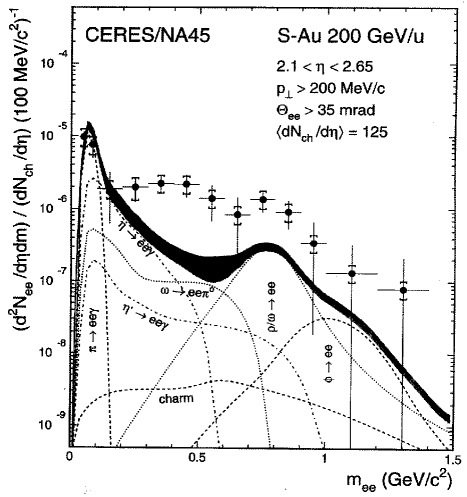
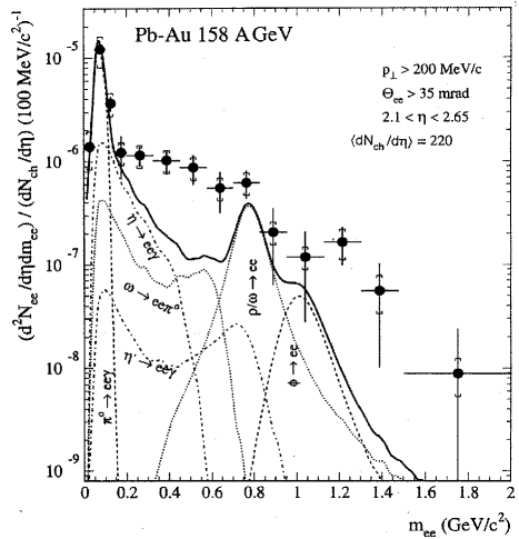
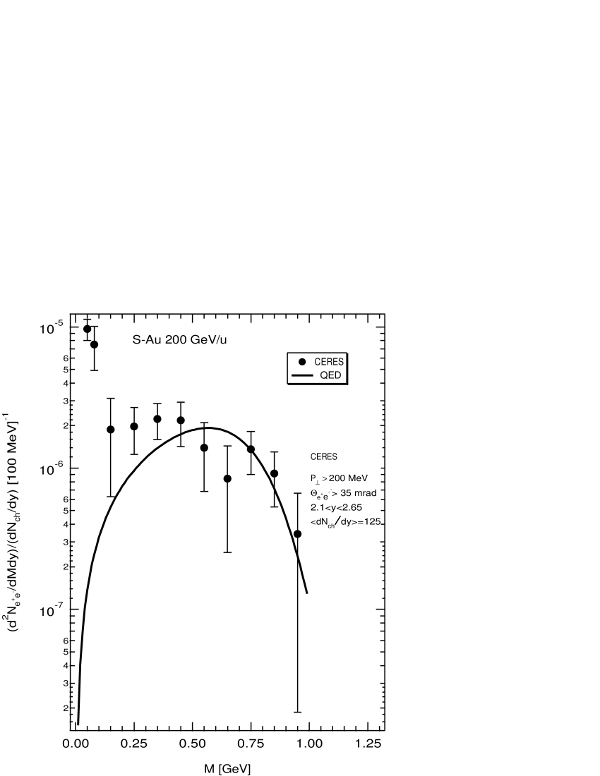
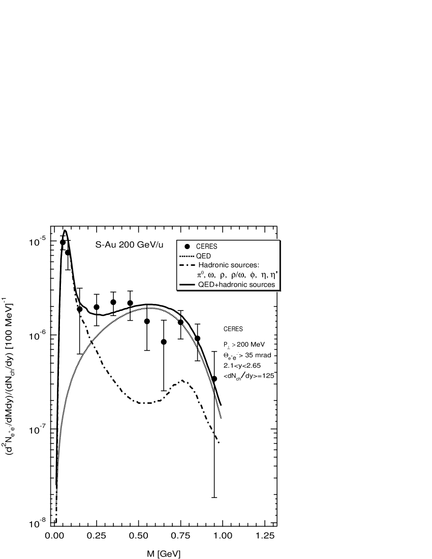
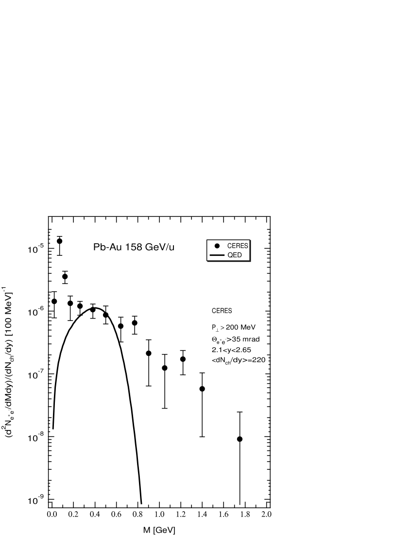
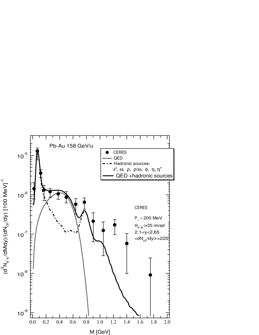
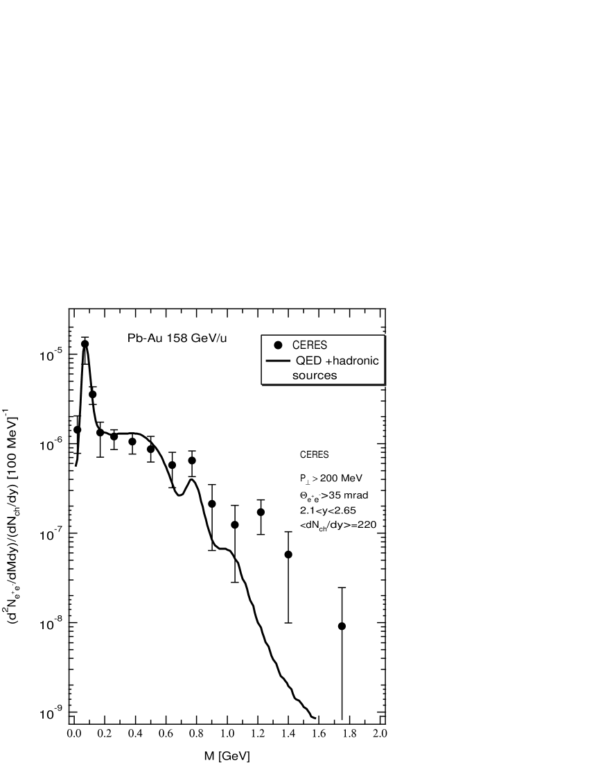
In particular three experiments have been conducted at the CERN-SPS in the last few years [3, 4, 5] to measure the yield of low mass ( GeV) pairs in such collisions in search of some signal of the QGP. In Fig.1 and in Fig.2 we report two typical observations of such experiments, showing a large yield of pairs in the mass region GeV and GeV, respectively), well in excess of that predicted as arising from conventional sources. Furthermore in experiments with a high energy proton beam impinging on a heavy nucleus [2] no such excess has been observed, suggesting that the source of the excess pairs lies in some peculiar aspect of the nucleus-nucleus interaction.
A wide consensus has formed so far around the hypotesis that the excess is due to some special manifestation of the QGP, and the important question is thus which peculiar QGP feature allows this hypotetical new state of matter to reveal its footprints in the form of abundant low mass pairs. As shown in Ref. [2], the situation is quite subtle and complicated, and the theory that appears now generally accepted [6] requires not only the production of an excess of vector mesons () over and above the normal yield in high energy pp-collisions, but also a substantial lowering of their masses, resulting from their propagation in a hot dense medium such as the QGP. And it is claimed [6], that simulations with relativistic transport models reproduce the experimental findings.
While we have no technical objection to the deductions and simulations of Li,Ko and Brown [6], we believe that the very notion of QGP, upon which this approach is based, is very arduous and difficult, and one that is quite unlikely to occur, due to the peculiar features of particle formation in high energy nucleon-nucleon scattering. A space-time analysis, in fact, of the process of particle production in high energy inelastic events [7] has made it rather plausible that most hadrons form well outside the interaction region. This surprising fact was first realized in the seventies, both theoretically and experimentally, when the fallacy of equating a nucleus to a “very dense bubble chamber” was clearly exposed. We note in passing that such is the physical behaviour predicted by the Fire-String (FS) model [8], where the quarks of the colliding Nuclei give rise to high mass string-like, unstable Hadronic states, the Fire-Strings which decay rather slowly into the jet-like structures universally observed in high energy hadronic final states. A detailed analysis, to be reported elsewhere [9], shows that even in Pb-Pb scattering at very high energies in the interaction region there never forms the hot dense matter which could (but how?) “thermalize” in a QGP, for the high energy density of the chromodynamic field that at the time of the collision exists in the interaction volume finds its way to the final state only much later, through a rather slow quark-pair creation process. And this appears to perfectly agree with a huge body of experimental information on the structure of hadronic states †††This can also explain the experimentally observed absence of measurable correlations between the hadronic jets produced in the decay of -pairs at the LEP..
It is for the above reasons that we have searched for a simpler, more realistic explanation of these interesting findings in a completely different direction, i.e. in the electromagnetic collective properties of a heavy nucleus, that are well known since a long time in the thouroughly studied phenomena related to the “giant resonances”, with frequency (A is the mass number) [10, 11]
| (1) |
and in this paper we wish to present a detailed analysis of the pair creation process induced by the “ weakly coherent” electromagnetic fields that are generated by such “giant resonances”.
The paper is organized as follows: Sect. contains the analysis of the structure of the coherent e.m. field generated by the coherent charge oscillations of the “giant resonances”, while in Sect. we compute the -pair production process in the “coherent” e.m. fields associated with the “giant resonances” of the colliding nuclei. The conclusions and outlook comprise Sect..
II The weak coherent e.m. field associated with the giant resonances.
Let us consider the e.m. vector potential generated by the zero-point modes, whose wave number is , the frequency of the giant resonance of the nucleus of mass number A, approximately given by (1).According to the discussion in Ref.[12], we may write in the Nucleus rest frame the vector potential within a coherence domain (CD) of radius :
| (2) |
where , (r=1,2) are the transverse polarization vectors and the associated amplitudes. Our basic idea is that the zero point amplitudes, as a consequence of their coupling to the coherent oscillations of the nucleons with frequency , become partly coherent, i.e. can be written as the sum:
| (3) |
of a coherent and an incoherent part, whose time averages are:
| (4) |
We look for a vector potential of the particularly simple form:
| (5) |
where r, , are the polar coordinates of the CD centered on the rest frame of the Nucleus, and is a unit vector to be determined by the transversality condition:
| (6) |
A simple analysis shows that:
| (7) |
From the representation (2) it requires little analysis to show that the coherent part of the amplitudes must have the form
| (8) |
where, according to (4), . The general analysis of electrodynamical coherence of Ref.[12] shows that the system oscillating Nucleus plus e.m. field stabilizes when the coherent amplitudes attain their maximum allowed values, thus we must have . Simple algebra is then required to write for the coherent e.m. field of a single Nucleus in its rest frame:
| (9) |
where
| (10) | |||||
| (12) |
In Table 1 we report the values of and for the interesting cases of S, Au and Pb.
As we have already mentioned, the physical origin and meaning of Eq.(9) is that the -independent modes of the e.m. field of frequency in the CD, through the interaction with the e.m. current generated by the giant resonance’s fluctuations, get “aligned” in a coherent superposition such as Eq.(9) and in so doing they minimize the total energy of the coupled matter-e.m. field system. As a result we can picture the nucleus A as surrounded by a “photon cloud” oscillating at the frequency of the giant resonance with a well defined amplitude (see Eq.(8)). It should be clear that the interaction of the “photon clouds” of the Heavy Ions, when they are brought to overlap at high energy, in the strong supercritical electric field that gets created in the collision, can induce the production of pairs of a well defined character, which we are now going to study.
III. THE PAIR PRODUCTION PROCESS.
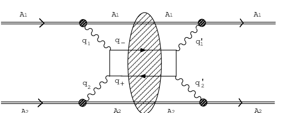
The process we wish to investigate is depicted in Fig.3 where the Heavy Ions and surrounded by their “photon clouds” described by and , the Fourier transforms of the boosted e.m. fields of Eq.(9), collide inelastically, while their “photon clouds” produce an pair through the well-known QED mechanism of “photon-photon pair creation”.
From the factorizable structure of the diagram in Fig.3 we can write:
| (13) |
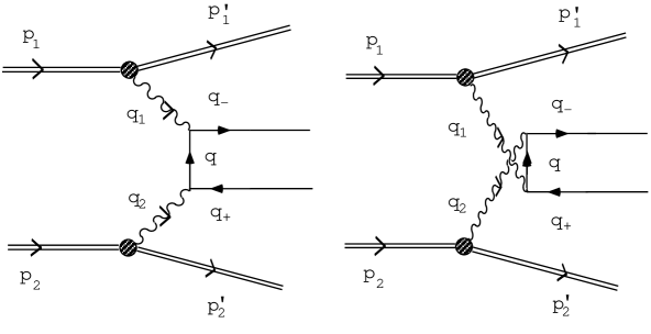
where the yield is calculated by squaring the amplitudes associated to the diagrams of Fig.4, which can be written as
| (14) |
where represents the well known leptonic part of the Feynman amplitude. The square of (14) can then be written
| (17) | |||||
where we can write for the generic Fourier transformed e.m. field:
| (19) |
From (9), in the Nucleus rest frame we have:
| (20) | |||||
| (21) |
Please note that in Fourier transforming we have extended the space-time integration to the finite (but large on a QCD scale) domain of the CD (). Thus the amplitudes are highly peaked functions around the values and , and this means that in the momentum-integrations in (LABEL:eq::produzione_esaltata_|S|_QUADRO) the important regions will be when and , their sharpness being controlled by the extent of and (note that the relative motion of the ions is ultrarelativistic). Thus, to lowest order in (where , a typical QCD scale), we may derive the following approximations:
| (22) | |||||
| (24) | |||||
| (25) | |||||
| (26) |
where
| (27) |
, and we have approximated the interaction space-time domain:
| (28) |
It is now straightforward to derive for the differential yield the following expression:
| (29) |
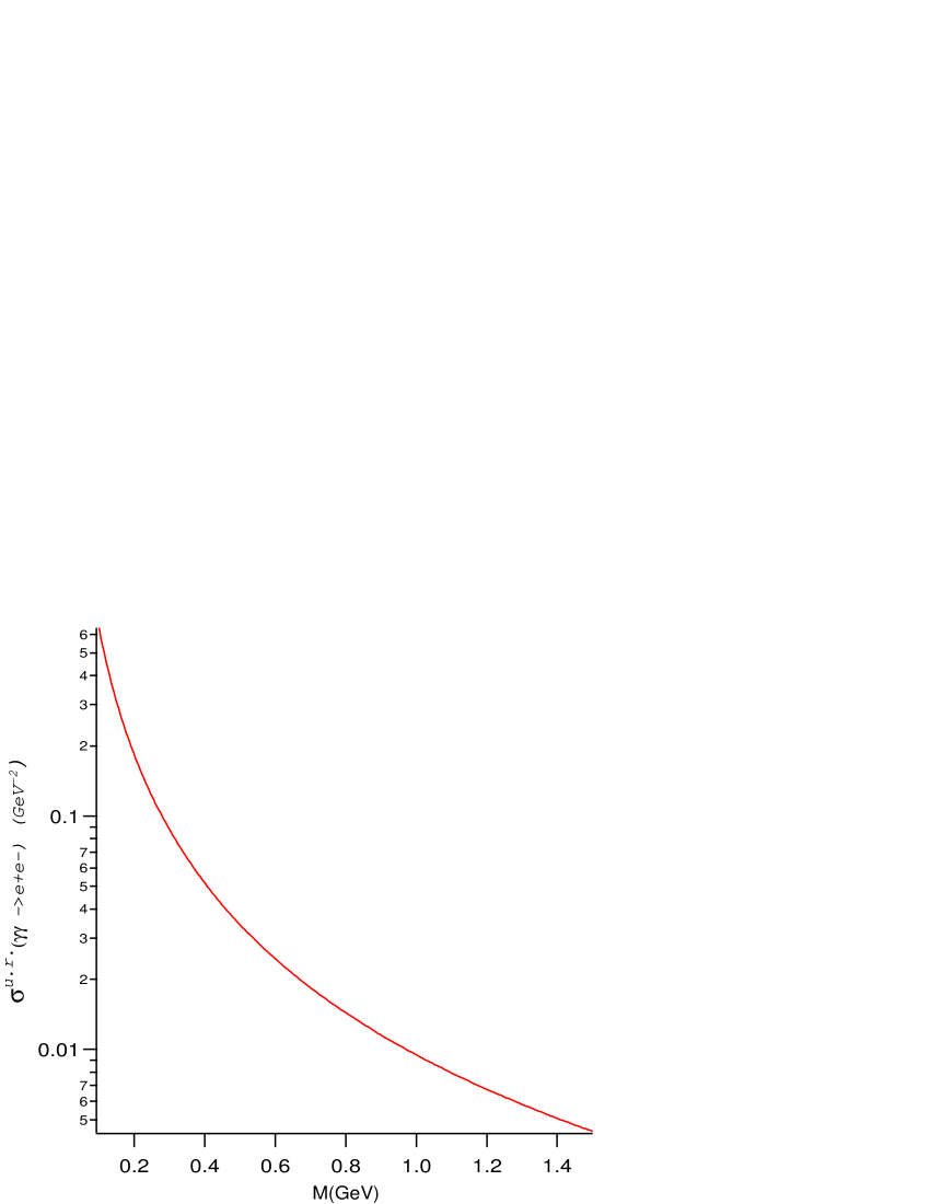
where and are the 4-dimensional Fourier transforms of the boosted “photon clouds”, and is the well-known differential cross section of annihilation in pairs of mass M. Fig.5 reports the shape of as a function of M [13], where is the total cross section in the ultrarelativistic limit. A simple approximate computation of Eq.(29) employs again the -like approximation:
| (30) |
where is the approximate normalization factor, and P is the Nucleus 4-momentum. Thus in the rest frame
| (31) |
approximating the - and - Fourier transforms of (9), both of which are steeply peaked at , the giant resonance frequency. With these simple approximations from (29) we derive:
| (32) |
where the “ form-factor” , ( is the pair rapidity in the CM), is given by
| (35) | |||||
where
| (36) |
The calculation of the “ form factor” can be best carried out by means of the Sudakov decomposition:
| (37) | |||||
| (38) | |||||
| (39) |
being the CM-energy of the colliding nucleons in the ultrarelativistic limit, and:
| (40) |
The result, which can be obtained in a straightforward manner, is
| (41) | |||||
| (42) |
where m is the nucleon mass and is the CM energy of the nucleon-nucleon collision.
It is clear that approximating sharp functions with -functions has produced the simple, but somewhat unrealistic result (42), yielding a sharp cut-off at , where E is the Laboratory energy of the impinging nucleon, . A more realistic and better approximation can be obtained by letting:
| (43) |
i.e. by replacing the -like approximation by a Gaussian whose parameter can be evaluated by equating the first-order expansion in of (43) and of , (see Eq.(21)). Thus we get
| (44) |
In this way the “ form-factor” is given by (neglecting a weak rapidity dependence):
| (47) | |||||
An approximate evaluation of this integral yields the following simple result:
| (48) |
III Conclusions and outlook.
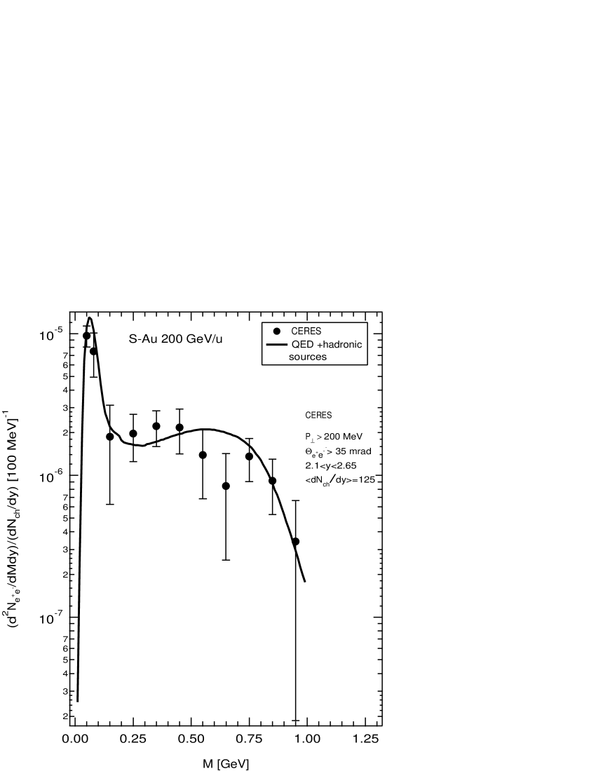
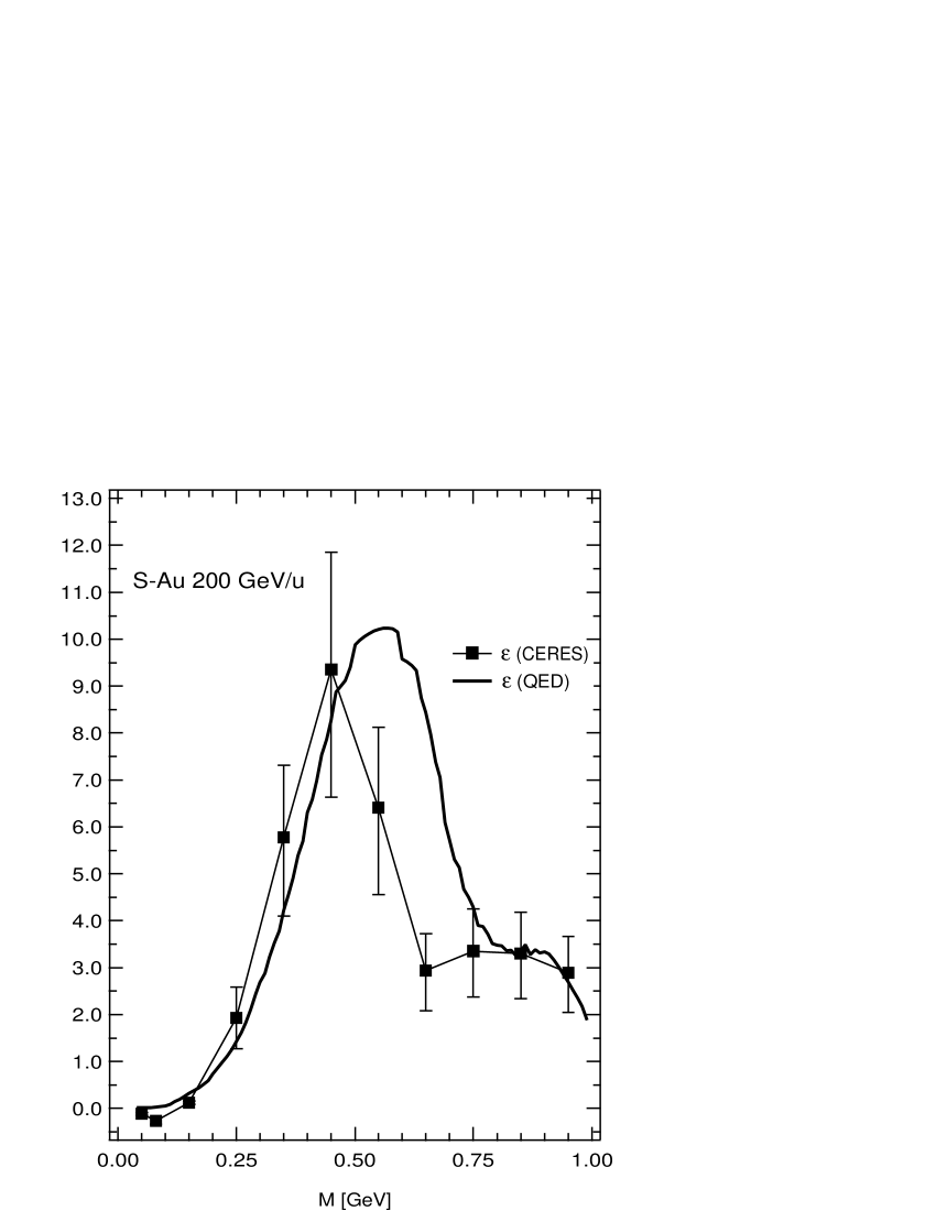
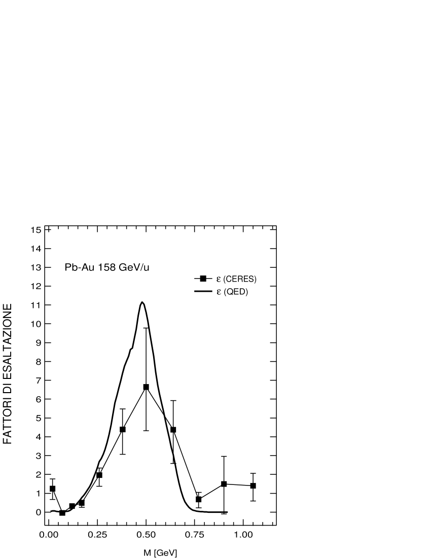
By feeding in the appropriate values of the frequencies and of the Lab-energies E in the formulae derived in the preceding Section, our results are compared with the experimental information in Figs.6,7,8,9, 10,11, for S-Au scattering at GeV per nucleon and Pb-Au at GeV per nucleon respectively. A good way to appreciate the success of our calculation is to compare the quantity:
| (49) |
with
| (50) |
This is done for S-Au in Fig.12 and for Pb-Au in Fig.13. In view of the parameterless nature of our calculation and of the approximations involved in it, we regard the agreement between theory and experiments really remarkable.
What physics lessons can we learn from all this? The first is that at very high energies the collisions between heavy ions can still provide us with interesting informations about the collective nuclear dynamics, and the pair production at low masses GeV) appears to bear witness to the importance and relevance of the collective excitations of heavy Nuclei in the generation of strong, coherent e.m. fields in which low-mass pair creation takes place. The conceptual as well as the calculational simplicity of our work is, in our view, a strong support of the validity of our physical explanation for the surprising excess observed by the mentioned experiments [3, 5].
Another equally important and relevant lesson is that another possible
signature for the
“mythical” QGP can be, most likely, explained away, our
computation leaving essentially no room for the -annihilation in low
mass pairs, that should characterize a hot, dense medium such as
QGP. Based on the discussion developed in the Introduction, this fact
represents a relevant corroboration of the fundamental ideas of QCD, that relegate all
phenomena of hadroproduction in the final state to a
long-distance, basically slow dynamics where the strong colour fields, created
by the rearrangements of the initial quarks in Fire-Strings [8], get
slowly converted into hadronic matter, which therefore appears in the
laboratory quite far (several Fermis at high energy) from the interaction
region. Naturally a good experimental evidence for the QGP, invalidating ideas
that have sprung from decades of hadronic physics, would pose several
fundamental problems not only to the FS-picture but also to the apparent lack
of the mechanisms needed to “thermalize” the QGP in the relatively short times
involved in high energy heavy-ion scattering. And, in this light, we are
particularly pleased by the results of this work.
Acknowledgments
We are indebted to dr. A.Drees for supplying us with the numerical data of the CERES S-Au measurements.
REFERENCES
- [1] H.Satz, Annu.Rev.Nucl.Part.Sci. 35, 245, (1985).
- [2] A.Drees, Nuclear Physics A630, 449c, (1998).
- [3] G. Agakichiev et al. (CERES Collaboration), Phys. Rev. Lett. 75, 1272, (1995).
- [4] T.Ullrich et al. Nuclear Physics A610, 317c, (1996).
- [5] G.Agakichiev et al., (CERES Collaboration), Phys. Letters, B 422, 405-412, (1998).
- [6] G.Q.Li, C.M.Ko, G.E.Brown and H.Sorge, Nucl. Phys. A611, 539, (1996).
- [7] A.Müller, in Proceedings of the 1981 ISABELLE Summer Workshop, edited by H.Gordon (BNL, Upton, New York, (1982)), pag.636. J.D. Bjorken, Phys.Rev. D27, 140, (1983).
- [8] L.Angelini, L.Nitti, M.Pellicoro, G.Preparata, G.Valenti, Riv. Nuovo Cimento 6,1, (1983). L.Angelini, L.Nitti, M.Pellicoro, G.Preparata, Phys.Rev. D41, 2081, (1990). G.Preparata, P.G.Ratcliffe, Phys.Lett. B345, 272, (1995).
- [9] G.Preparata, R.Alzetta, T.Bubba, G.Liberti, G.Mileto, D.Tarantino, in preparation.
- [10] F. E. Bertrand, Nuclear Physics, A354, 129c, (1981).
- [11] W.Greiner, J.A.Maruhn, Nuclear Models, Springer, 1996.
- [12] G.Preparata, QED Coherence in Matter, World Scientific, 1995.
- [13] W.Greiner, J.Reinhardt, Quantum Electrodynamics, Springer, 1996.
Table 1
| Nucleus | A | ||
|---|---|---|---|
| Au | 32 | 23 | 27 |
| S | 197 | 13.4 | 46 |
| Pb | 207 | 13.1 | 47 |
List of Figures
lof