Phenomenology of Large $N_{c}$ QCD

Abstract

These lectures are designed to introduce the methods and results of large $N_{c}$ QCD in a presentation intended for nuclear and particle physicists alike. Beginning with definitions and motivations of the approach, we demonstrate that all quark and gluon Feynman diagrams are organized into classes based on powers of $1/N_{c}$. We then show that this result can be translated into definite statements about mesons and baryons containing arbitrary numbers of constituents. In the mesons, numerous well-known phenomenological properties follow as immediate consequences of simply counting powers of $N_{c}$, while for the baryons, quantitative large $N_{c}$ analyses of masses and other properties are seen to agree with experiment, even when “large” $N_{c}$ is set equal to its observed value of 3. Large $N_{c}$ reasoning is also used to explain some simple features of nuclear interactions.

I Motivations and Fundamentals

The purpose of these lectures is to define, explain, and exhibit the methods of large $N_{c}$ QCD for phenomenologists of both the nuclear and particle bent. Several excellent reviews on this topic exist in the literature, each with a different emphasis, and to each I am indebted for aspects of the pedagogy presented in the current work. Witten’s article on large $N_{c}$ baryons[1], one of my favorite papers, actually begins with a review of large $N_{c}$ mesons. Chapter 8 in Coleman’s Aspects of Symmetry[2] covers the development of large $N_{c}$ through 1980. Many of the newer developments with baryons are included in Manohar’s 1997 Les Houches lectures[3] and Jenkins’ review[4].

I assume that initially many readers may find the notion of large $N_{c}$ to be a rather exotic and unlikely approach to studying the strong interactions, as it seemed to me when I began to learn it some years ago. As always with an unfamiliar topic, it is important to start with clear definitions and motivations. We begin with the assertion that QCD-like theories possess a peculiar limit in which the physics of the strong interactions becomes much simpler. It is the so-called large $N_{c}$ limit, in which the number of color charges, $N_{c}$ (= 3 in our universe) is taken as a free parameter (i.e., the gauge group is SU($N_{c}$)), and one considers the limit $N_{c}\to\infty$. Physical quantities are then considered in this limit, where corrections appear at relative orders $1/N_{c}$, $1/N_{c}^{2}$, etc., the $1/N_{c}$ expansion. Shortly after its discovery by ’t Hooft[5] in 1974, the method was applied to mesons with many qualitative successes in explaining phenomenology. However, it has only been in the past several years that much success has come in the analysis of baryons, with much of it quantitative.

However, before a detailed discussion of these very interesting points, it is important to consider some simple but incisive questions. How does large $N_{c}$ work? What does it predict? And, perhaps most importantly, is it believable?

In this section, we discuss how and why large $N_{c}$ should work, and how it is implemented at the very basic level of QCD, in terms of quarks and gluons. To start with, the very notion of the approach creates an interesting paradox: How can increasing the number $N_{c}$ of degrees of freedom actually simplify the strong interaction problem? It is certainly true that the detailed interactions of any particular quark or gluon become much more complicated if one insists on solving the theory exactly. To illustrate this point, let us introduce two analogies; we shall come to appreciate that they represent the way large $N_{c}$ works for mesons and baryons, respectively. The first analogy is that of a particle moving in a complicated potential, one that requires many parameters for a complete description, and the second is the many-body problem in mechanics. Both are difficult because of the large number of available dynamical degrees of freedom. However, if increasing the number of degrees of freedom permits one to consider only collective couplings in a systematic way, then the form of the dynamics simplifies. In the first analogy, the potential might be decomposable into a simple dominant piece (which nonetheless originates from a large number of more fundamental interactions), while the other portions are subleading perturbations. In the second, statistical mechanics describes the system’s gross features in terms of just a few collective quantities, such as temperature or volume; fluctuations about these values are highly suppressed.

With these qualitative arguments in mind, what is special about the large $N_{c}$ limit of QCD in particular?

1. It is a perturbative QCD expansion. Compare QCD to QED; why does the latter work so much better? Obviously, $\alpha_{\rm QED}\sim 1/137$ is a perturbative expansion parameter, while $\alpha_{\rm QCD}=O(1)$ at hadronic energy scales is clearly not perturbative. At high energies, $\alpha_{\rm QCD}$ runs to smaller values due to asymptotic freedom, but one would prefer a perturbative parameter that works at all scales. In fact, only one such parameter is known to exist for QCD-like theories, namely, $1/N_{c}$.

2. Physics simplifies in the large $N_{c}$ limit. As we show presently, certain classes of Feynman diagrams dominate over others in physical amplitudes, and this organization leads to many interesting simplifications. For example, we shall see that a color singlet $\bar{q}q$ pair always appears at leading order in $1/N_{c}$ as a single meson.

3. It provides an explanation of phenomena hard or impossible to explain in field theory. For example, OZI suppression and the physical dominance of resonant-mediated processes are consequences of large $N_{c}$, as we shall see.

4. It seems to work, even for $N_{c}=3$. This is perhaps the most startling reason; indeed, one might expect that $1/N_{c}=1/3$ is too large to be a reasonable expansion parameter. However, such an objection may be answered in two ways. One is described by Coleman[2] as Witten’s “wisecrack”: Consider $\alpha_{\rm QED}=e^{2}/4\pi\sim 1/137$, which leads to $e\sim 0.3\sim 1/3$. If $1/N_{c}$ is too large an expansion parameter, why don’t we say the same thing about the QED charge $e$? Turning the argument around, one can find cases where the expansion parameter turns out to be $1/N_{c}^{2}\sim 1/10$, which is more satisfactory to some critics of the approach. However, I prefer a much more pragmatic answer, which is just that one should perform a given calculation with $N_{c}$ a free parameter, set it to 3 at the end of the day, and see for oneself whether or not the factors of 3 are supported by the experimental measurements. The ultimate justification of any approach in this view is whether it successfully explains physical observations and can be tested in new situations.

Before proceeding, consider the evidence that $N_{c}=3$ in our universe; it is important to check that there is nothing fundamentally immutable about this particular value that would impede consideration of larger $N_{c}$. Historically, the original reason for the invention of color[6] was to explain how fermionic baryons could have a completely symmetric spin-flavor-space wavefunction, as suggested by experiment. A canonical example is $\Delta^{++}(J_{z}=+3/2)=(u\!\uparrow)(u\!\uparrow)(u\!\uparrow)$, which is completely symmetric under spin-flavor indices. Since the spatial wavefunction for this low-lying state is expected to be completely symmetric, so is the combined spin-flavor-space wavefunction, and therefore one requires a new degree of freedom with (at least) 3 values completely antisymmetric under quark exchange.

The experimental confirmation of the color idea came with the measurement of the ratio

$$R_{\rm hadron}\equiv\sigma(e^{+}e^{-}\to{\rm hadrons})/\sigma(e^{+}e^{-}\to\mu^{+}\mu^{-})$$ (1)

away from thresholds for new flavor production, which is found, as originally predicted[7], to be a factor of 3 larger than what one would predict from a colorless quark theory. Similarly, perturbative QCD, in those high-energy kinematic regimes where it is believed valid, only gives results in agreement with experiment when one sets $N_{c}=3$. Furthermore, the calculated rate for $\pi^{0}\to\gamma\gamma$, which matches experiment, includes a factor of $N_{c}=3$.

Finally, the Standard Model is only renormalizable if the particle content is chosen to eliminate the possibility of chiral anomalies. In particular, since quark charges are known from deep inelastic scattering experiments to be integral multiples of 1/3, one can show that chiral anomalies cancel only for the choice $N_{c}=3$. For universes with larger values of $N_{c}$, the cancellation of anomalies is accomplished by adjusting the quark charges accordingly, to be integral multiples of $1/N_{c}$.

With these lessons in mind, let us consider the valence structure of hadrons in large $N_{c}$. In order to make progress, we first make the crucial assumption that color confinement occurs for arbitrarily large $N_{c}$; otherwise, such a universe bears no resemblance to ours, since then free colored hadrons or even free quarks can be abundant. Such an assumption is not required, of course, since the physical extrapolation from $N_{c}=3$ to $N_{c}\to\infty$ might lead from a confining to a nonconfining phase at some value of $N_{c}>3$, but then the large $N_{c}$ limit would be of little phenomenological value since we have no empirical knowledge of nonconfining strong interactions.

Mesons of valence flavor structure $\bar{q}_{1}q_{2}$ with color indices $\alpha$, $\beta$ for arbitrary $N_{c}$ have the normalized wavefunction

$$\frac{1}{\sqrt{N_{c}}}\,(\bar{q}_{1})_{\alpha}(q_{2})^{\beta}\,\delta^{\alpha}{}_{\!\beta},$$ (2)

where $\delta^{\alpha}{}_{\!\beta}$ serves to combine the $\bar{q}q$ pair into a color singlet. The salient point is that mesons still have the quantum numbers of a system with a single quark and a single antiquark for arbitrary $N_{c}$. Baryons, on the other hand, are built in analogy with the $N_{c}=3$ observation that fermionic states with completely symmetric spin-flavor-space wavefunctions require at least as many colors as quarks. On the other hand, once we specify that there are $N_{c}$ colors, SU($N_{c}$) group theory requires a minimum of $N_{c}$ colored quarks to form a color singlet. Therefore, large $N_{c}$ baryons require exactly $N_{c}$ valence quarks. Given the valence quarks $q_{1},q_{2},\ldots,q_{N_{c}}$, the normalized wavefunction including color indices $\alpha_{1},\alpha_{2},\ldots,\alpha_{N_{c}}$ is

$$\frac{1}{\sqrt{N_{c}!}}\,(q_{1})^{\alpha_{1}}(q_{2})^{\alpha_{2}}\cdots(q_{N_{c}})^{\alpha_{N_{c}}}\,\epsilon_{\alpha_{1}\alpha_{2}\cdots\alpha_{N_{c}}}.$$ (3)

Furthermore, only odd $N_{c}$ produces fermionic baryons, since each of the $N_{c}$ quarks has spin 1/2. The large $N_{c}$ limit may be used equally well to consider even-$N_{c}$ bosonic baryons, but of course these are not phenomenologically relevant.

We are now ready to consider large $N_{c}$ QCD itself, as developed by ’t Hooft. To the non-initiate who has been told of large $N_{c}$ results but never taught its origins, the whole idea might still seem a bit like necromancy. But like any good magic show, the essential predictive power of large $N_{c}$ just comes from trap doors (topology) and mirrors (group theory).

Let us begin with the usual particle content of QCD with the color gauge group SU($N_{c}$). Quarks carry a color index in the fundamental representation of the group, which means that the standard representation is a column vector $q^{\alpha}$ with $N_{c}$ components, one for each color. Diagrammatically, it is represented by an arrowed line. Antiquarks carry a color index in the fundamental conjugate, or anti-fundamental, representation, and therefore appear in standard form as a row vector $q_{\alpha}$ with $N_{c}$ components. They are also drawn as arrowed lines, but the (anti-) color flow is understood to be opposite the direction of the arrow. Gluons, which appear in the adjoint representation of SU($N_{c}$), carry one color and one anti-color index, and appear in standard form as traceless $N_{c}\times N_{c}$ matrices $A^{\alpha}{}_{\!\beta}$, which can be drawn as two parallel lines whose arrows point in opposite directions. This is called ’t Hooft’s double-line notation; it is actually extraordinarily convenient in capturing the color physics, because exact color conservation implies that color lines are continuous, while the confinement assumption means that color lines form only closed loops. The three QCD vertices in double-line notation are depicted in Fig. 1.

The double-line notation is particularly useful as a guide to developing an understanding of how the QCD gauge parameter, $g_{s}$ ($s$ = strong), scales as $N_{c}\to\infty$. In fact, as ’t Hooft argued in his original paper[5], QCD Green functions only have smooth, finite limits as $N_{c}\to\infty$ if $g_{s}\propto 1/\sqrt{N_{c}}$. Since this is such a central result in the analysis to come, we prove the claim in detail below. However, let us ponder for a moment why such a result is interesting. Given that $g_{s}\propto 1/\sqrt{N_{c}}$, one can show that certain classes of Feynman diagrams dominate over others, in possessing fewer powers of $1/N_{c}$, an organization known as large $N_{c}$ power counting. The dominant class of graphs is denoted planar, which means that these graphs can be drawn in the double-line notation in the plane of paper, with any quark line (if one is present) placed on the perimeter, and with color lines arranged to cross only at vertices. Each nonplanarity, as will be shown, costs a suppression factor of $1/N_{c}^{2}$. Moreover, diagrams with no internal quark loops dominate over the others, in that each internal quark loop costs a factor of $1/N_{c}$. So, in summary, large $N_{c}$ counting provides an organization of all Feynman diagrams into a well-defined and countable hierarchy of classes.

We now present a proof of ’t Hooft’s scaling of $g_{s}$. Vertices typically fall into three types. There are bilinears that create $\bar{q}q$ pairs from the vacuum, and are accompanied by $g_{s}^{0}$; let there be $V_{2}$ of these current insertions. Each of $V_{3}$ trilinear ($\bar{q}qg$ or $ggg$) vertices includes $g_{s}^{1}$, while each of $V_{4}$ quartic vertices includes $g_{s}^{2}$. Confinement requires that the $C$ color lines in the digram completely close; then one may choose any of the $N_{c}$ colors to appear on each loop, providing a combinatoric factor of $N_{c}^{C}$. In total, then, the diagram scales as

$${\cal A}\propto g_{s}^{V_{3}+2V_{4}}N_{c}^{C}.$$ (4)

Since the diagram has no external lines by color confinement, both ends of each propagator $P$ terminate on a vertex:

$$2P=\sum_{n}nV_{n}=2V_{2}+3V_{3}+4V_{4}.$$ (5)

Defining the total number of vertices

$$V=\sum_{n}V_{n}=V_{2}+V_{3}+V_{4},$$ (6)

one has

$${\cal A}\propto g_{s}^{2P-2V}N_{c}^{C}.$$ (7)

It is very fruitful to use the double-line notation to interpret the diagram as a polyhedron, much like a geodesic roof. Each color loop $C$ becomes a face, where each propagator $P$ is an edge and each vertex $V$ of the diagram is also a vertex of the solid figure. Then each quark loop, which possesses one less color line than if it were replaced by a (double-line) gluon loop, may be thought of as a missing face, or topological boundary $B$, while each nonplanar line may be interpreted as a handle (since it represents one edge forced to pass in front of another but not meet at a vertex), or topological unit of genus $G$. We relate these features to topological objects so that we may now use a famous theorem due to Euler: For each orientable figure, there is a topological invariant called the Euler character $\chi_{E}$ satisfying

$$\chi_{E}=C-P+V=2-2G-B.$$ (8)

Therefore,

$${\cal A}\propto(g_{s}^{2}N_{c})^{C}\left[(g_{s}^{2}N_{c})^{-1}\,N_{c}\right]^{2-2G-B}.$$ (9)

The first term still depends on the particular diagram, while the second has a purely topological power. Now observe that, if $g_{s}$ falls off faster than $1/\sqrt{N_{c}}$, then diagrams of any given topology with the fewest color loops, and hence a minimal number of gluons, dominate; but this is a trivial theory, in that only valence diagrams are important. Clearly the gluon degrees of freedom are vital to understanding the strong interaction, so we reject this possibility. On the other hand, if $g_{s}$ falls off slower than $1/\sqrt{N_{c}}$, then diagrams of any given topology with the most color loops dominate; but this is a nonsense theory, for one can always add more color loops to diagrams of a given topology, and in this scenario one could make no predictions at all. However, we know that this is not the case, since perturbative QCD in high-energy regimes works well. We conclude that $g_{s}\propto 1/\sqrt{N_{c}}$ is the only nontrivial, sensible large $N_{c}$ scaling, giving the result

$${\cal A}\propto N_{c}^{2-2G-B},$$ (10)

meaning that the large $N_{c}$ counting of any particular diagram is purely topological. Since this is the case, for any given diagram one may add an arbitrarily large number of planar gluons and remain within the same topological class, i.e., the diagram maintains the same large $N_{c}$ counting. However, each additional quark loop or nonplanar gluon adds one unit to $B$ or $G$, leading to an additional $1/N_{c}$ or $1/N_{c}^{2}$ suppression, respectively.

Another (although actually equivalent) way to demonstrate $g_{s}\propto 1/\sqrt{N_{c}}$ is to start with the QCD renormalization group equation,

$$\mu\frac{dg_{s}(\mu)}{d\mu}=-b_{0}\frac{g_{s}(\mu)^{3}}{16\pi^{2}}+O(g_{s}^{5}(\mu)),$$ (11)

where $b_{0}=(11N_{c}-2N_{f})/3>0$, with $N_{f}$ the number of light quark flavors, and the positivity of $b_{0}$ being the reason we know that QCD is asymptotically free. Let us rescale $g_{s}=\bar{g}_{s}N_{c}^{-1/2+\epsilon}$, with $\bar{g}_{s}$ finite as $N_{c}\to\infty$. Then (11) reads

$$\mu\frac{d\bar{g}_{s}(\mu)}{d\mu}=-\frac{1}{3}\left(11-2\frac{N_{f}}{N_{c}}\right)\frac{\bar{g}_{s}^{3}(\mu)}{16\pi^{2}}N_{c}^{2\epsilon}+O(\bar{g}_{s}^{5}(\mu)).$$ (12)

We immediately see that, if $\epsilon<0$, $\bar{g}_{s}$ is constant and $g_{s}$ instantly runs to zero for $N_{c}$ large (assuming that the theory has a perturbative limit), leading to a trivial theory of valence diagrams only; on the other hand, if $\epsilon>0$, $\bar{g}_{s}$ runs infinitely fast, making a nonsense theory with no meaningful predictions. Again, we conclude that only $g_{s}\propto 1/\sqrt{N_{c}}$ leads to a nontrivial and sensible theory.

We conclude this section by illustrating in Figs. 2 and 3 the large $N_{c}$ counting in the three different approaches: counting powers of $g_{s}$ and $N_{c}$, counting features of the equivalent polyhedra, and counting topological invariants. These examples should provide the reader with hands-on experience with the theorems we have considered.

II Mesons in the $1/N_{c}$ Expansion

Having shown that the large $N_{c}$ limit of QCD is only nontrivial and sensible if $g_{s}\propto 1/\sqrt{N_{c}}$, and that Feynman diagrams involving quarks and gluons fall into classes labeled by powers of $N_{c}$ with planar diagrams at leading order, what have we gained? Certainly, the observed strongly interacting particles are hadrons rather than quarks and gluons, and so if there were no obvious relation between the two pictures — beyond the valence quark model, which unlike large $N_{c}$ contains no explicit gluons — large $N_{c}$ would hold little phenomenological interest. But in fact one can derive an elegant and simple large $N_{c}$ relationship between hadrons and their fundamental QCD constituents. In this section, we consider this derivation and its consequences for mesons.

A good starting point for these discussions is to consider the particle spectrum of large $N_{c}$. In our $N_{c}=3$ world, one observes conventional mesons with the quantum numbers of $\bar{q}q$, baryons with the quantum numbers of $qqq$, and more recently, hybrid mesons[8] with the quantum numbers of ($\bar{q}q$ + gluons). On the other hand, one might equally well expect to see glueballs, which are defined as mesons containing all gluons and no valence quarks, exotic multiquark mesons with the quantum numbers of ($\bar{q}q$ + extra $\bar{q}q$ pairs), exotic baryons with the quantum numbers of ($qqq$ + extra $\bar{q}q$ pairs), and hybrid baryons, with the quantum numbers of ($qqq$ + glue). Members of the latter class have not yet been observed, and with the exception of hybrid baryons, large $N_{c}$ provides an explanation.

To see how it works, first consider QCD two-point diagrams as depicted in Figs. 2, 3. The current $J$ creates a $\bar{q}q$ pair from the QCD vacuum at some spacetime point, the quarks propagate and interact for some interval, and then the pair is annihilated by a current $J^{\dagger}$. We ask, what kinds of hadrons can appear in the intermediate state? Equivalently, using our confinement assumption, we want to discover what color-singlet combinations of quarks and gluons are revealed if we cut the diagram at any convenient place. We claim that, to leading order in $1/N_{c}$, cutting such a diagram leads only to a single $\bar{q}q$ meson — no multiquark mesons, no glueballs.

The proof of this statement relies on planar diagrams with no internal quark loops (which alone eliminates multiquark mesons from our discussion) dominating in the $1/N_{c}$ expansion. Typical planar diagrams in the double-line notation are those exhibited in Fig. 2. The unique feature possessed by planar diagrams and no others is that, when cut, each color index appears adjacent to its corresponding anticolor index. That is, one cuts through an entire color loop before passing to the next one. In terms of fields, the equivalent (perhaps nonlocal) operator has color structure

$$\bar{q}_{\alpha_{1}}A^{\alpha_{1}}{}_{\!\alpha_{2}}A^{\alpha_{2}}{}_{\!\alpha_{3}}\cdots A^{\alpha_{n-1}}{}_{\!\alpha_{n}}\,q^{\alpha_{n}}.$$ (13)

In terms of the generators of color indices, one may use the usual Gell-Mann matrices $\lambda^{a}$ to expose the underlying structure

$$\left(\lambda^{a_{1}}\right)^{\alpha_{1}}{}_{\!\!\!\alpha_{2}}\left(\lambda^{a_{2}}\right)^{\alpha_{2}}{}_{\!\!\!\alpha_{3}}\cdots\left(\lambda^{a_{n}}\right)^{\alpha_{n-1}}{}_{\!\!\!\alpha_{n}}.$$ (14)

Now one uses a little SU($N_{c}$) group theory to complete the proof. A particularly convenient way to do this is to exhibit the commutation relations obeyed by the generators:

$$\left[\lambda^{a},\lambda^{b}\right]=2if^{abc}\lambda^{c},\hskip 20.00003pt\left\{\lambda^{a},\lambda^{b}\right\}=\frac{4}{N_{c}}\delta^{ab}+2d^{abc}\lambda^{c}.$$ (15)

Combining these,

$$(\lambda^{a})^{\alpha_{1}}{}_{\!\alpha_{2}}(\lambda^{b})^{\alpha_{2}}{}_{\!\alpha_{3}}=\frac{2}{N_{c}}\delta^{ab}\delta^{\alpha_{1}}{}_{\!\alpha_{3}}+\left(d^{abc}+if^{abc}\right)(\lambda^{c})^{\alpha_{1}}{}_{\!\alpha_{3}},$$ (16)

where the first term, which is color singlet, is suppressed by $1/N_{c}$, while the second term, which is color adjoint like the original gluons, is of leading order, $O(N_{c}^{0})$. By induction, every string of gluon fields is color adjoint to leading order, and therefore the only way to make a leading-order color singlet from the diagram is to take the operator $\bar{q}AA\cdots Aq$ as an irreducible whole. The conclusion is that only a single meson, and no glueballs or multiquark mesons, appear at leading order in $1/N_{c}$.

This important result can now be used to prove a wide variety of consequences. Since each planar two-point diagram with a $\bar{q}q$ pair appears as a single meson, the sum of planar two-point diagrams with momentum transfer $p^{2}$ must also equal a sum of meson propagators,

$$\mbox{\rm Planar diagram sum}=O(N_{c}^{1})=\sum_{n}\frac{f_{n}^{2}}{p^{2}-m_{n}^{2}},$$ (17)

where $f_{n}$, the $n$th meson decay constant, is defined as the transition amplitude between meson state $n$ and the vacuum through the current $J$. Using that $p^{2}$ is arbitrary and that the equality must hold for any (sufficiently large) value of $N_{c}$, one finds that $m_{n}^{2}=O(N_{c}^{0})$ and $f_{n}=O(\sqrt{N_{c}})$. Furthermore, for $p^{2}$ very large, the diagram must approach its perturbative QCD result, $\sim\ln(p^{2}/\mu^{2})$, where $\mu$ is the renormalization point. However, no finite sum of factors $f_{n}^{2}/(p^{2}-m_{n}^{2})$ produces a logarithm in $p^{2}$, so the number of meson states in large $N_{c}$ must be infinite. Since one may restrict this calculation to diagrams of a given fixed $J^{PC}$, it is also true that the number of mesons of any particular quantum numbers is also infinite.

One may continue in this fashion to consider three-, four-, and higher-point functions. The diagrams in these cases resemble those of the two-point function, except for the inclusion of more current insertions, and thus are all $O(N_{c}^{1})$. However, unlike in the two-point diagram, there is now more than one way to collect the quark and gluon fields into color singlets. For example, for the three-point function, each of the three current insertions may create a meson, which annihilate at a trilinear meson vertex (Fig. 4). Alternately, one current insertion may create two mesons, which propagate to the remaining two insertions. The three-point diagram is then given by

$$\sum_{1,2,3}\frac{f_{1}f_{2}f_{3}\cdot(\mbox{\rm 3-meson vertex})}{(p_{1}^{2}-m_{1}^{2})(p_{2}^{2}-m_{2}^{2})(p_{3}^{2}-m_{3}^{2})}+\sum_{2,3}\frac{(\mbox{\rm Amplitude to create 2 mesons})\cdot f_{2}f_{3}}{(p_{2}^{2}-m_{2}^{2})(p_{3}^{2}-m_{3}^{2})}.$$ (18)

Using that $m_{n}^{2}\sim N_{c}^{0}$, $f_{n}\sim\sqrt{N_{c}}$, one discovers that the 3-meson vertex scales as $1/\sqrt{N_{c}}$, while the amplitude to create 2 mesons scales as $N_{c}^{0}$.

Diagrams with more current insertions allow for more types of internal meson vertices, and the $N_{c}$ scaling behavior of each type of vertex can be derived inductively. For example, meson vertices from the four-point function can be obtained by using results from the two- and three-point functions. In general, given an $m$-point function, each possible $n$-point diagram, $n<m$, is required to appear with the large $N_{c}$ scaling derived in a previous induction step (a statement of unitarity) with all possible permutations of meson propagators (a statement of crossing symmetry). One finds in this way the general results that both the $m$-meson vertex and the amplitude to create $m$ mesons from the vacuum scale as $N_{c}^{1-m/2}$. This important result appears to have been first obtained by Veneziano[9].

Such a scaling implies immediately that mesons are free, since the propagator, i.e., the “two-meson vertex,” scales as $N_{c}^{0}$, and therefore neither blows up nor vanishes as $N_{c}\to\infty$, while the $1/\sqrt{N_{c}}$ scaling of the three-meson vertex, and the additional $\sqrt{N_{c}}$ suppression for each additional meson, implies that mesons are stable — a remarkable result! But, could mixing with possible exotic states spoil this reasoning? We now discuss the fate of exotics to show that this does not occur.

First consider glueballs; for simplicity, depict those with only two valence gluons, whose two-point diagrams resemble those of Figs. 2 and 3, except that the exterior quark is replaced by a gluon. Then all the large $N_{c}$ counting is the same as before, except that the single color line of the quark is replaced by the double line of the gluon. Therefore, each diagram is a factor of $N_{c}$ larger, so that the planar diagrams scale as $N_{c}^{2}$. The same proof as for mesons shows that these diagrams are dominated by the one-glueball state, and so one finds that the masses and decay constants of glueballs scale as $N_{c}^{0}$ and $N_{c}^{1}$, respectively. Continuing with the same logic as before, the $g$-glueball vertex scales as $N_{c}^{2-g}$.

As for glueball-meson mixing, the simplest planar diagram for the process is exhibited in Fig. 5. Converting it to double-line format, we find two color loops and two factors of $g_{s}$, so that the diagram scales as $N_{c}^{1}$. Using our previous results for the glueball and meson decay constants of $N_{c}^{1}$ and $\sqrt{N_{c}}$, which appear at the current insertions, we see that the glueball-meson coupling scales as $1/\sqrt{N_{c}}$, meaning that glueballs and mesons do not mix at leading order. Therefore, glueballs and mesons are separately free, stable particles as $N_{c}\to\infty$, with the combined result that the $g$-glueball, $m$-meson vertex for $m>0$ scales as $N_{c}^{1-g-m/2}$.

Next consider multiquark mesons, e.g., those with valence quantum numbers $\bar{q}q\bar{q}q$. These are created by current insertions of the form $J=\bar{q}q\bar{q}q(x)$, as depicted in Fig. 6. To leading order in $1/N_{c}$, the color loops close either as (1,2), (3,4) or (1,4), (2,3). This means that the diagram has two distinct closed color loops and scales as $N_{c}^{2}$; however, we know from our previous reasoning that each such loop is a single meson to leading order in $1/N_{c}$. To create a single meson with $\bar{q}q\bar{q}q$ quantum numbers requires an irreducible color loop, such as (1,2,3,4) or (1,4,3,2); however, such a diagram scales as $N_{c}^{1}$ and is thus subleading. We conclude that multiquark mesons are suppressed in $1/N_{c}$.

Finally, we turn our attention to hybrid mesons. From the previous paragraphs, one might expect that we shall dispose of these as well. But, in fact, they are present in the large $N_{c}$ limit[10]. To see this diagrammatically, consider hybrids of valence structure $\bar{q}qg$; one simple planar diagram representing their propagation is given in Fig. 7$a$. One finds two color loops and two factors of $g_{s}$, meaning that such diagrams scale as $N_{c}^{1}$, the same as the leading conventional valence meson diagrams as in Figs. 2, 3. In particular, one finds that hybrid mesons have masses of $O(N_{c}^{0})$ and decay constants of $O(\sqrt{N_{c}})$, exactly like those of conventional mesons. As for meson-hybrid mixing, one leading diagram is depicted in Fig. 7$b$, which has two color loops and two factors of $g_{s}$, thus scaling as $N_{c}^{1}$. Of course, the symmetries of spacetime require that the conventional and hybrid mesons in this case must share the same quantum numbers. Using that both conventional and hybrid mesons have decay constants scaling as $\sqrt{N_{c}}$, one sees that the meson-hybrid coupling is $O(N_{c}^{0})$, so that the two mix freely in large $N_{c}$. An equivalent observation is that all mesons in large $N_{c}$ are expected to have a finite hybrid component, and the large $N_{c}$ limit sheds no light on the mystery of why almost all observed mesons have only the quantum numbers of conventional mesons.

It should also be noted that hybrids with exotic (non-$\bar{q}q$) quantum numbers (such as the newly-observed $1^{-+}$) do not mix with conventional mesons at leading order in $1/N_{c}$, but are nonetheless not hard to create. The leading three-point diagrams allow for one or more of the current insertions to have exotic quantum numbers, which means that the process of exotic meson production occurs at the same order in $N_{c}$ as that of conventional mesons. Glueballs, on the other hand, are harder to create from meson sources and slower to decay in the large $N_{c}$ limit; we leave the verification of these facts as an opportunity for the reader to experiment with double-line diagrams.

In summary, our analysis of the large $N_{c}$ meson spectrum teaches that, for the phenomenology of conventional mesons, one may ignore glueballs, multiquark states, and hybrids with exotic quantum numbers. On the other hand, hybrids with conventional quantum numbers should be treated just like conventional valence mesons. The general multiparticle vertex for $g$ glueballs, $m$ mesons, and $h$ hybrids scales as

$$N_{c}^{1-g-m/2-h/2},$$ (19)

for $m>0$ or $h>0$. When $m=h=0$, the exponent is $2-g$. The physical mesons, which contain a hybrid component, are free, since the propagator scales as $N_{c}^{0}$; stable, since the 3-meson vertex is $O(1/\sqrt{N_{c}})$, and non-interacting, since meson-meson scattering, i.e. the 4-meson vertex, is $O(1/N_{c})$.

In general, one concludes that diagrams with the fewest mesons allowed tend to dominate physical processes. This immediately gives a field-theoretic explanation of the dominance of resonance-mediated decays and the existence of excited mesons narrow enough to measure. Although one could imagine an alternative strong interaction in which every mesonic process with a substantial amount of energy release simply produced a spray of pions and nothing else, the real strong interaction very definitely produces a rich and complex spectrum of observable resonances. Large $N_{c}$ QCD gives an extraordinarily economical explanation for this basic observation.

One success of the large $N_{c}$ limit is the OZI rule[11], that meson processes requiring the annihilation or $\bar{q}q$ pairs, or equivalently, the presence of an all-glue intermediate state, are phenomenologically suppressed. The canonical example is the decay of the $\phi(1020)$ meson, which is believed to have the valence structure $\bar{s}s$. It decays into a $K\bar{K}$ pair, for which there is almost no phase space ($2m_{K}\sim 1$ GeV) 83% of the time, but only 17% of the time into $\rho\pi$, $\pi\pi\pi$, and other nonstrange modes, for which there is much more available phase space. Apparently, $\bar{s}s$ annihilation is suppressed, and large $N_{c}$ offers a very simple explanation: A decay like $\phi\to\bar{K}K$ may be represented with a standard, leading-order ($O(N_{c}^{1})$) three-point diagram as we have discussed, but annihilating the strange quark closes its quark color loop and requires another to create the light hadrons in the final state. Since each quark loop costs a factor of $1/N_{c}$, the leading OZI-suppressed diagrams inherit this suppression.

The observed fact that mesons appear in nonets of flavor SU(3) rather than octets, i.e., that the flavor octet and singlet mesons tend to mix and have comparable masses, is another success of large $N_{c}$. The canonical example is $\eta(547)$ and $\eta^{\prime}(958)$, which are the mass eigenstates of mixing between a flavor singlet $\eta_{1}$ and flavor octet $\eta_{8}$; a priori, the $\eta_{1}$ could have turned out much heavier than $\eta_{8}$. However, one can show that diagrams differentiating between their masses either break SU(3), large $N_{c}$, or both. To see this, begin in the SU(3) flavor limit where $u$, $d$, and $s$ quarks are not distinguished. Then all planar two-point diagrams such as in Fig. 2 contribute equally to both masses, but a diagram with pure glue intermediates contributes to $m^{2}(\eta_{1})$ alone, since gluons, like $\eta_{1}$, are flavor singlets. Because the latter diagrams are suppressed by $1/N_{c}$, one concludes that terms symmetric in SU(3) that distinguish the masses — which a priori could have been large — are in fact suppressed by $1/N_{c}$ effects:

$$m^{2}(\eta_{1})-m^{2}(\eta_{8})=O\left(1/N_{c},\,m_{s}\right).$$ (20)

As a final example of mesonic applications of large $N_{c}$, consider the famous ’t Hooft model[13]. By definition, the ’t Hooft model is large $N_{c}$ QCD in 1 space and 1 time dimension (1+1). Although it is called a model, it is actually a full-fledged quantum field theory that is exactly soluble, in that all hadronic Green functions may be obtained entirely in terms of quark degrees of freedom. For example, one can compute meson masses precisely in terms of quark masses. Furthermore, the only asymptotically free states in the theory are confined, color-singlet hadrons, which appear in an infinite tower of increasing masses.

So, although we assumed confinement in large $N_{c}$ QCD in 3+1 dimensions, it appears to be an immediate consequence in 1+1. Such a result might be expected based upon naive dimensional analysis. For, consider the momentum space potential derived from a single gluon exchange propagator in the instantaneous approximation:

$$V(\mbox{\boldmath$q$})\sim 1/\mbox{\boldmath$q$}^{2},$$ (21)

and Fourier transform to position space. In 3+1 dimensions, one has $V(\mbox{\boldmath$r$})\sim 1/r$, the usual Coulomb interaction, which is asymptotically free as $r\to\infty$; in 1+1, $V(\mbox{\boldmath$r$})\sim r$, which confines as $r\to\infty$. That the confining potential survives relativistic and field theory corrections is, however, nontrivial.

The ’t Hooft model is soluble precisely because of the two features of its definition. Large $N_{c}$ guarantees that nonplanar gluons and virtual quark loops are suppressed, while working in 1+1 allows one to choose gauges for the gluon field such that gluon-gluon couplings vanish. Such terms arise in minimal substitution from the commutator $[A_{\mu},A_{\nu}]$ term; working in a gauge such that one of the two components of $A$ vanishes guarantees that the commutator does also. The only remaining diagrams are “rainbow” and “ladder” types (Fig. 8) and these can be summed using “bootstrap”-type Schwinger-Dyson equations, essentially the same trick that is used to sum the geometric series.

Performing this summation for the Green function of a $\bar{q}q$ system, one obtains the meson wavefunction $\phi$ in terms of the ’t Hooft equation,

$$\mu_{n}^{2}\phi_{n}^{M\overline{m}}(x)=\left(\frac{M_{R}^{2}}{x}+\frac{m_{R}^{2}}{1-x}\right)\phi_{n}^{M\overline{m}}(x)-\int^{1}_{0}dy\,\phi_{n}^{M\overline{m}}(y)\,\Pr\frac{1}{(y-x)^{2}},$$ (22)

where the available kinematic invariants are the quark masses $M$ and $m$, the resultant meson mass eigenvalue $\mu$, and the 1+1 analogue $x$ of the deep inelastic variable $x_{\rm BJ}$, defined by

$$x\equiv\frac{p_{Q}^{0}+p_{Q}^{1}}{p_{\rm mes}^{0}+p_{\rm mes}^{1}}\in[0,1].$$ (23)

Qualitatively, $x$ and $1-x$ represent the fraction of meson momentum carried by the quark and antiquark, respectively. The quark masses are renormalized by

$$m_{R}^{2}=m^{2}-\frac{g_{s}^{2}N_{c}}{2\pi},$$ (24)

from which we note that the 1+1 strong coupling $g_{s}$ actually has dimensions of mass, and using that $g_{s}\sim 1/\sqrt{N_{c}}$, it is natural to describe masses in units of $g_{s}\sqrt{N_{c}/2\pi}$. Such a quantity acts in the same way in 1+1 as $\Lambda_{\rm QCD}$ in 3+1, in that it distinguishes “heavy” from “light” quarks. The ’t Hooft equation is known to possess an infinite tower of solutions, labeled by $n=0,1,2,\ldots$, which alternate in parity ($P=(-1)^{n+1}$). As $n\to\infty$, the meson masses scale as $\mu_{n}^{2}\to\pi^{2}n$. Since $x$ is bounded between 0 and 1, the ’t Hooft equation is qualitatively similar to the quantum mechanical problem of a particle in a box.

The utility of the ’t Hooft model is that it can be used to study difficult problems of QCD that have not been fully solved in 3+1, such as the meson form factors, deep inelastic scattering, and the saturation of hadronic rates by partonic diagrams. For example, consider[14] the nonleptonic weak decay of a meson containing a heavy quark into lighter mesons. As the heavy quark mass $M$ is increased, the light antiquark and gluon degrees of freedom should exert less and less influence on the decay of the heavy quark, and eventually the process should be well described by the diagram of free heavy quark weak decay. Since one can compute both the hadronic and partonic decay rates in the ’t Hooft model, the two can be compared directly. The result is Fig. 9, in which one sees that the two rates rapidly approach one another for large $M$.

III Baryons in the $1/N_{c}$ Expansion

Recalling from Sec. I that baryons for quarks of $N_{c}$ colors have the quantum numbers of $N_{c}$ quarks, one is immediately faced with the dilemma of how to understand the physics of a system with $N_{c}\to\infty$ constituents. A particularly simple and elegant paradigm for dealing with this situation is the mean-field Hartree-Fock baryon picture due to Witten[1], in which each quark moves in the field caused by the other $N_{c}-1$ quarks acting collectively. To lowest order in $1/N_{c}$, this field is static — after all, a system of $N_{c}-1$ quarks possesses a great deal of inertia compared to a single quark. Then each quark in the ground state satisfies the same field-theoretical wave equation (which, for very heavy quarks, reduces to the Schrödinger equation); although the exact form of this wave equation depends upon the details of QCD and is therefore unknown, much can be said from its existence and its large $N_{c}$ scaling properties.

For starters, since each quark in the ground state satisfies the same wave equation, each one has the same wavefunction $\phi(\mbox{\boldmath$r$})$, which we claim scales as $N_{c}^{0}$. For the scaling claim to be sensible, the potential due to the other $N_{c}-1$ quarks in which each of the $N_{c}$ quarks moves must also scale as $N_{c}^{0}$, or equivalently, baryon diagrams must never give interaction energies more than $O(N_{c}^{1})$. To see that this is true, one must first understand large $N_{c}$ counting for baryon diagrams. The potential comes from diagrams with connected interactions such as those depicted in Fig. 10. In addition to factors of $N_{c}$ from $g_{s}\propto 1/\sqrt{N_{c}}$ and color loops, one has combinatoric factors due to the presence of $N_{c}$ quark lines. For example, diagrams involving two quarks can be chosen in ${}_{N_{c}}C_{2}=N_{c}(N_{c}-1)/2=O(N_{c}^{2})$ ways, diagrams involving three quarks can be chosen in ${}_{N_{c}}C_{3}=N_{c}(N_{c}-1)(N_{c}-2)/6=O(N_{c}^{3})$ ways, and so forth. The three diagrams in Fig. 10 are all seen to appear at $O(N_{c}^{1})$, and so are among the leading-order diagrams. It is not hard to prove that no diagrams are of lower order, and that internal quark loops and nonplanar gluons (See Appendix A) cost factors of $1/N_{c}$, meaning that a consistent large $N_{c}$ counting scheme compatible with the Hartree-Fock picture does indeed exist for the baryons.

Since $\phi(\mbox{\boldmath$r$})$ is the same for each quark in the baryon, it follows that each quark has the same charge distribution and occupies the same space; therefore, baryons remain the same size as $N_{c}\to\infty$. In contrast, large $A$ nuclei grow in size with $A$ because of the phenomenological saturation of nuclear forces. Whereas large $N_{c}$ baryons and large $A$ nuclei both have masses proportional to the numbers of constituents $N_{c}$ and $A$, respectively, large $N_{c}$ baryons are like rigid containers with radius $\propto N_{c}^{0}$ and density $\propto N_{c}^{1}$, while large $A$ nuclei are like close-packed spheres with density $\propto A^{0}$ and radius $\propto A^{1/3}$. This is why the Hartree-Fock picture works for baryons but not nuclei.

Within the Hartree-Fock picture it is possible to obtain large $N_{c}$ behavior for common physical processes. For example, consider (Fig. 12) baryon-baryon ($BB$) and baryon-meson ($BM$) scattering. In the $BB$ case, one may choose from among $N_{c}$ quarks in each baryon, while at least one gluon is typically required to keep both baryons color singlets and conserve momentum, providing a factor $(g_{s}/\sqrt{N_{c}})^{2}$. The amplitude for the process thus scales as $N_{c}^{1}$. In the $BM$ case, the counting proceeds as before, except that one loses one of the $N_{c}^{1}$ combinatoric factors, meaning that the amplitude scales as $N_{c}^{0}$. Do these factors make sense? For $BB$, since baryon masses are $O(N_{c}^{1})$, an amplitude of $O(N_{c}^{1})$ leads, via the usual textbook formulae, to a nonvanishing, finite ($O(N_{c}^{0})$) cross-section. For $BM$, since meson masses are $O(N_{c}^{0})$, the cross-section formulae lead to the scattering of the meson — but not the baryon — with $O(N_{c}^{0})$ probability; the physical picture in this case is the meson scattering from a fixed potential center.

Although the Hartree-Fock picture provides a simple archetype for the large $N_{c}$ baryon, its value is limited since it only describes the leading-order $N_{c}$ counting for a given process. This was also the case for the mesons, but now with $N_{c}$ constituents in the baryon, it becomes possible to perform studies of subleading effects in $1/N_{c}$, which involve some subset of the quarks acting collectively. In the next two subsections, we shall discuss the two known techniques for studying the subleading $1/N_{c}$ structure of baryons: consistency condition and spin-flavor algebra methods. Both make use of an operator basis acting upon the baryon states, and so the bulk of the $1/N_{c}$ suppressions is carried by the operators. The remainder of this lecture is dedicated to explaining these two schemes and their phenomenological results. The consistency condition approach turns out to be related closely to an operator analysis based on the Skyrme model[15], while the spin-flavor method turns out to be closely related to operator analysis performed in the quark model.

A Consistency Conditions

The starting point of this scheme is to consider baryon-meson scattering not in terms of quarks, but rather hadrons. Suppose that the meson is a $\pi$, which, as a Nambu-Goldstone boson of chiral symmetry, couples to baryons derivatively through the isovector axial vector current $A^{\mu a}=\bar{q}\gamma^{\mu}\gamma_{5}\tau^{a}q$, where $\tau$ is an isospin Pauli matrix. The scattering process consists of two insertions of $A^{\mu a}$ on the baryon line, which can occur in two orderings as depicted in Fig. 13. Since each quark in the baryon can couple to $A^{\mu a}$, one expects its matrix elements to be $O(N_{c}^{1})$, and the full vertex is written as

$$\left<B^{\prime}\left|\bar{q}\gamma^{i}\gamma_{5}\tau^{a}q\right|B\right>\partial_{i}\pi^{a}/f_{\pi}\equiv\tilde{g}N_{c}X^{ia}_{B^{\prime}B}\partial_{i}\pi^{a}/f_{\pi},$$ (25)

where the coupling constant $\tilde{g}$ and the operator $X^{ia}$, each of $O(N_{c}^{0})$, are defined by this equation. Note that only the space components of $A^{\mu a}$ appear in the leading term of the nonrelativistic expansion of the quark bilinear, and only these are needed here, since at leading order in $1/N_{c}$ the baryon may be taken at rest throughout the process. This implies also that the $\pi$ scatters elastically from the baryon, and so in the first diagram in Fig. 13 the baryon is off-shell by an amount $E_{\pi}$, whereas in the second the amount is ($-E_{\pi}$). Therefore, since the derivatives produce factors of pion momenta $k$, the amplitude for the two diagrams together is

$${\cal M}=\frac{iN_{c}^{2}\tilde{g}^{2}k^{i}k^{\prime\,j}}{f_{\pi}^{2}E_{\pi}}\left[X^{jb},X^{ia}\right]_{B^{\prime}B}.$$ (26)

Using that $f_{\pi}\propto\sqrt{N_{c}}$, ${\cal M}$ naively appears to scale as $N_{c}^{1}$, rather than $N_{c}^{0}$ as concluded previously. One evades this conundrum by noting that many baryon states may appear on the intermediate line, i.e., are inserted between the two $X$’s in the commutator; then cancellations can render the matrix elements of the commutator $O(1/N_{c})$ even though matrix elements of each $X$ individually are $O(N_{c}^{0})$, as pointed out by Gervais and Sakita in 1984[16]. Such cancellations are called consistency conditions.

The mathematics behind this approach was developed in the 1960s as one of many methods to study strong interactions, and is generically called the method of induced representations of a contracted spin-flavor algebra. In order to explain this intimidating term, we first consider what is meant by a contracted algebra. In essence, it means that one or more generators of an algebra is scaled so as to change the commutation relations. For example, perform a $1/N_{c}$ expansion of the operator $X$:

$$X^{ia}=X_{0}^{ia}+\frac{1}{N_{c}}X_{1}^{ia}+\cdots,$$ (27)

in terms of which we have seen that

$$\left[X_{0}^{ia},X_{0}^{jb}\right]=0.$$ (28)

By virtue of its defining indices $i$ and $a$, $X^{ia}$ is a spin-1, isospin-1 tensor, and therefore by definition satisfies

$$\left[J^{i},X_{0}^{jb}\right]=i\epsilon^{ijk}X_{0}^{kb},\hskip 20.00003pt\left[I^{a},X_{0}^{jb}\right]=i\epsilon^{abc}X_{0}^{jc}.$$ (29)

Also, as usual,

$$\left[J^{i},J^{j}\right]=i\epsilon^{ijk}J^{k},\hskip 20.00003pt\left[I^{a},I^{b}\right]=i\epsilon^{abc}I^{c},\hskip 20.00003pt\left[I^{a},J^{i}\right]=0,$$ (30)

which are the defining relations of spin-flavor SU(2) $\times$ SU(2). How do the commutation relations with $X_{0}$ alter the algebra? To see what happens, compare the algebra defined by (28)–(30) with that of spin-flavor SU(4). In addition to containing SU(2) $\times$ SU(2), SU(4) also has commutation relations with the combined spin-flavor generator $G^{ia}\equiv J^{i}\otimes I^{a}$,

$$\left[J^{i},G^{ja}\right]=i\epsilon^{ijk}G^{ka},\hskip 20.00003pt\left[I^{a},G^{jb}\right]=i\epsilon^{abc}G^{ic},$$ (31)

$$\left[G^{ia},G^{jb}\right]=\frac{i}{4}\left(\epsilon^{ijk}\delta^{ab}J^{k}+\epsilon^{abc}\delta^{ij}I^{c}\right).$$ (32)

Note that the two algebras become the same if one writes

$$X_{0}^{ia}=\lim_{N_{c}\to\infty}G^{ia}/N_{c},$$ (33)

and works to leading order in $1/N_{c}$, so that the right hand side of the commutator $[G,G]$ vanishes. This is the contraction of the spin-flavor algebra. One immediately concludes that, due to the contraction, the smaller spin-flavor symmetry SU(2) $\times$ SU(2) is promoted to the larger symmetry SU(4), at leading order in $1/N_{c}$. For three light flavors $u$, $d$, $s$, for which the flavor symmetry is SU(3), one finds SU(2) $\times$ SU(3) $\to$ SU(6) at leading order. This enlargement of the symmetry due to the contraction allows one to find a number of new relations among physical quantities. In fact, the SU(6) spin-flavor symmetry[17] has been known to work well for baryons — but rather poorly for mesons — since the 1960s; in large $N_{c}$, one sees at last a field-theoretic reason how such a symmetry might arise.

Next, a representation of an algebra is induced when one attempts to specify the quantum numbers of a given state as classified according to a generator of the algebra, and discovers that other quantum numbers must be specified to label the state completely. This happens, for example, when one classifies the irreducible representations of the Lorentz group; once a given inertial frame (i.e., set of boost coordinates) is chosen, one finds that there still exists a “little group” of transformations needed to specify the representation, which correspond physically to rotations in that frame: Choosing the frame induces the full representation. In the present case, once one specifies eigenvalues of the operator $X_{0}$, one finds[18] that there remains a “little group” of generators with quantum numbers $K$, $k$, like those of angular momentum, $K=0,1,2,\ldots$, and $k=-K,-K+1,\ldots,K-1,K$. That is, choosing $X_{0}$ induces an irreducible representation specified by the states $\left|\right.X_{0},K,k\left.\right>$.

Of course, $X_{0}$ is not an intuitively familiar physical operator, so one then projects the states $\left|\right.X_{0},K,k\left.\right>$ onto the space of states $\left|\right.I,I_{3},J,J_{3},K\left.\right>$. Certainly isospin and spin are familiar, but what of the induced quantum number $K$? As shown by Dashen, Jenkins, and Manohar[19], $K$ turns out to have the same properties as the number of strange quarks in the baryon, $K=N_{s}/2$. The relation mentioned earlier between the consistency condition approach and the Skyrme model, namely, that the group theory associated with the Skyrme model is precisely that obtained from the consistency condition method, is also discussed in that work.

The consistency condition (28) and others like it derived from multiple pion or kaon scattering with nucleons provide fertile ground for phenomenological analysis. One simply plugs an operator possibly contributing to a given physical process into the consistency relations, sees if it is satisfied, and if not, discards the operator. This process builds a $1/N_{c}$ expansion for a given operator, and hence for physical quantities. For example, one can derive the pion-baryon coupling constant relation

$$g_{\pi NN}/g_{\pi N\Delta}=3/2+O(1/N_{c}^{2}),$$ (34)

or show that $X^{ia}_{1}$ in (27) is proportional to $X^{ia}_{0}$, meaning that effectively

$$X^{ia}=X^{ia}_{0}+O(1/N_{c}^{2}),$$ (35)

so that nonstrange axial currents have no $O(1/N_{c})$ corrections, or show that the masses of nonstrange baryons of spin $J$ in the same spin-flavor multiplet, such as the nucleons and $\Delta$’s, are first split at relative order $J^{2}/N_{c}^{2}$[20], i.e.,

$$M=N_{c}\left[c_{0}+c_{1}\frac{J^{2}}{N_{c}^{2}}+O\left(\frac{1}{N_{c}^{4}}\right)\right],$$ (36)

where $c_{0}$ and $c_{1}$ are unknown coefficients of $O(N_{c}^{0})$. These relations arise simply because the operators that would violate them are disallowed by the consistency conditions. Phenomenology seems to agree well with this analysis; in the examples given, $g_{\pi N\Delta}/g_{\pi NN}=1.48$ experimentally, while the relative mass difference between the nucleon and $\Delta$ is about $(1232-940){\rm MeV}/\frac{1}{2}(1232+940){\rm MeV}=0.27$, which is very close to $[J_{\Delta}(J_{\Delta}+1)-J_{N}(J_{N}+1)]/N_{c}^{2}=0.33$ for $N_{c}=3$.

A large body of additional work has been performed using the consistency condition approach. To sample but a few, baryon magnetic moments[21], orbitally excited[22, 23], and hybrid[24] have been studied in this scheme.

B Spin-flavor Algebra

In the consistency condition approach just discussed, we saw that a full combined spin and flavor symmetry arises from the separate spin and flavor symmetries to leading order in $1/N_{c}$, due to the group contraction. Why not, then, describe all operators acting upon the baryons in terms of operators with definite SU($2F$) properties, where $F$ is the number of light quark flavors, acting upon the sum of the quarks? That is, the operator basis in SU(6), for example, is defined as

$$J^{i} \equiv q^{\dagger}_{\alpha}\left(\frac{\sigma^{i}}{2}\otimes\openone\right)q^{\alpha},$$ (37)

$$T^{a} \equiv q^{\dagger}_{\alpha}\left(\openone\otimes\frac{\lambda^{a}}{2}\right)q^{\alpha},$$ (38)

$$G^{ia} \equiv q^{\dagger}_{\alpha}\left(\frac{\sigma^{i}}{2}\otimes\frac{\lambda^{a}}{2}\right)q^{\alpha},$$ (39)

where $\sigma^{i}$ are the usual Pauli spin matrices, $\lambda^{a}$ denotes Gell-Mann flavor matrices, and the index $\alpha$ sums over all $N_{c}$ quark lines in the baryons. One can readily show that $J$, $T$, and $G$ satisfy an SU(6) algebra analogous to the SU(4) algebra Eq. (31).

An important point to realize is that, although baryons are described in this approach in terms of $N_{c}$ “quarks,” a large $N_{c}$ constituent quark model[25] is not assumed. Indeed, recalling the lesson from Sec. II that valence and hybrid mesons mix freely, one might well expect the same for hybrid baryons[24]. However, the only assumption really used to perform this operator analysis is that baryons for large $N_{c}$ continue to have the same total quantum numbers as those obtained from an $N_{c}$ quark system. Then, a “quark” in the sense of Eq. (37) is not the same as the dynamical entity of the QCD Lagrangian, but rather a group-theoretical object representing one part in $N_{c}$ of the physical baryon. The two definitions coincide when the quarks are taken very heavy, so that their interactions with the internal gluons become less important in determining the baryon structure.

It was shown by Manohar[26] that results of the Skyrme model obtained from its operator structure (and hence obtained from the consistency condition approach) and those obtained from the operator structure of the quark model (and hence obtained from the spin-flavor algebra approach) coincide as $N_{c}\to\infty$. Therefore, either approach is equally good from the mathematical point of view for describing large $N_{c}$ baryons. Moreover, the total result for any given quantity must be the same regardless of which approach one uses, which is simply the statement that the physical result must be independent of mathematics. One sees that the consistency condition and spin-flavor algebra methods differ for a given physical quantity only by a reorganization of $1/N_{c}$ corrections.

The initial work on the baryon $1/N_{c}$ expansion in the spin-flavor algebra approach was performed by Carone, Georgi, and Osofsky[27] and Luty and March-Russell[28]. The basic results of these analyses is that many of the old SU(6) static relations between baryonic matrix elements are recovered by means of an operator expansion in $1/N_{c}$. That is, any given physical operator ${\cal O}^{(m)}$ that scales as $N_{c}^{m}$ may be written in the form

$${\cal O}^{(m)}=N_{c}^{m}\sum_{n,p,q}c_{n}\biggl{(}\frac{J^{i}}{N_{c}}\biggr{)}^{p}\biggl{(}\frac{T^{a}}{N_{c}}\biggr{)}^{q}\biggl{(}\frac{G^{jb}}{N_{c}}\biggr{)}^{n-p-q},$$ (41)

where it is understood that spin and flavor indices are to be contracted in such a way as to agree with the transformation properties of ${\cal O}^{(m)}$.

The factor of $1/N_{c}$ accompanying each $J$, $T$, and $G$ reflects the fact that the matrix elements of these operators can often add coherently over the $N_{c}$ quarks and thus can be as large as $O(N_{c}^{1})$. In fact, this was the central problem with the spin-flavor algebra method: One hopes to describe a given quantity with some small number of operators, but if a number of the operators in (41) have matrix elements of $O(N_{c}^{1})$, where can it justifiably be truncated? Before addressing this problem directly, it is useful to consider the nature of the baryon multiplets in this approach.

Since we are making use of representations of the symmetry group SU($2F$) for operators acting upon the baryons, the most convenient description for the baryons is in terms of multiplets of SU($2F$). Recall that this is the symmetry of independent rotations in all spin SU(2) and flavor SU($F$) coordinates, under which the ground state baryons appear to fill a completely symmetric representation. It is very convenient to describe the representations in terms of Young tableaux, in which each quark, which appears in a fundamental representation of SU($2F$), is represented by a single box. Boxes arranged in a row indicate symmetrization of the corresponding SU($2F$) indices, while boxes arranged in a column indicate antisymmetrization. The tableau for the completely symmetric SU($2F$) multiplet of $N_{c}$ quarks is a row of $N_{c}$ boxes, as in the first line of Fig. 14; using standard group theory techniques, this representation can be decomposed into a tower of component ${\rm SU}(F)_{\rm flavor}\times{\rm SU(2)}_{\rm spin}$ representations, as indicated in the succeeding lines of Fig. 14. Each Young tableau in this tower has $N_{c}$ boxes. If you are familiar with the old SU(6) theory of baryons, then you will recognize the special case of $N_{c}=3$, $F=3$ as the decomposition

$${\bf 56}=\left({\bf 8},J=\frac{1}{2}\right)\oplus\left({\bf 10},J=\frac{3}{2}\right).$$ (42)

The significance of this result is twofold: First, the number of SU($F$) $\times$ SU(2) representations increases as $N_{c}$ is increased from its physical value of 3, and second, the individual SU($F$) multiplets themselves become much larger as $N_{c}$ is increased beyond three. This point is illustrated in Figs. 15 and 16 for the case of three light flavors; note how the familiar SU(3) octet (which contains the nucleons) and the decuplet (which contains the $\Delta$ resonances) are obtained from shrinking the representation down to $N_{c}=3$.

Let us now return to the conundrum of where to truncate the expansion (41). We see that working with $N_{c}$ large generates an enormous number of baryon states, but we are only interested in the phenomenology of those with which we are familiar, i.e., that already exist for $N_{c}=3$, which we denote physical baryons. Where do they appear within the large multiplets of Figs. 15, 16? The mathematics alone allows for a great deal of freedom for placing the physical states, but the usefulness of (41) as a perturbative expansion in $1/N_{c}$ imposes constraints on this choice. For example, since the expansion breaks down if $J=O(N_{c}^{1})$ or $I=O(N_{c}^{1})$, we take physical baryons to have $J=O(N_{c}^{0})$ and $I=O(N_{c}^{0})$. As for the strangeness content, consider for example the top-right entry of the multiplet Fig. 15; its spin-flavor structure is $uud$ in a total spin-1/2, isospin-1/2 state (just as for an $N_{c}=3$ proton) plus $(N_{c}-3)/2$ $ud$ pairs, each combined into spin-0, isospin-0 quantum numbers. It is tempting to identify this state as the $N_{c}>3$ analogue of the proton, and one may do this by fiat; indeed, in light of our statements above, the physical proton should have $J=I=1/2$ even for $N_{c}>3$. Apart from the top-right state, the physical proton might occupy any of a number of sites in Fig. 15 that lie directly below this one. However, each of these states contains a number of $s$ quarks, which are heavier than $u$ and $d$ quarks, and therefore these baryons should be heavier than those on the top row. If the physical proton contains some valence $s$ quarks, it decays weakly to some other lighter baryon, a process that opens up a phenomenological Pandora’s box. One does not encounter any of these or similar problems if one identifies the physical baryons to lie at the tops of Figs. 15 and 16.

Even taking these assignments into account, some of the operators, such as $T^{4,5,6,7}$ and $G^{ia}$, can still give matrix elements of $O(N_{c})$, even when evaluated only on the physical baryons. All is not lost, however, since we have not to this point made full use of the mathematics. Since the operators can be thought of as a set of vectors spanning the space of physical observables, it must be that there are only as many independent operators as independent observables. One can obtain a number of operator reduction rules[29] based upon both the structure of the spin-flavor algebra SU($2F$) and properties particular to the completely symmetric ground-state representation.

To see how this works, collect the SU($2F$) generators into a uniformly normalized set:

$$\Lambda^{A}\equiv\left\{\left(\sigma^{i}/2\otimes\openone\right)/\sqrt{F},\,\left(\openone\otimes\lambda^{a}/2\right)/\sqrt{2},\,\sqrt{2}\left(\sigma^{i}/2\otimes\lambda^{a}/2\right)\right\}\to{\rm Tr\,}\Lambda^{A}\Lambda^{B}=\frac{1}{2}\delta^{AB}.$$ (43)

Then two simple operator reduction relations are

$$q^{\dagger}_{\alpha}(\openone\otimes\openone)q^{\alpha} = N_{c}\openone,$$ (44)

$$\left(q^{\dagger}_{\alpha}\,\Lambda^{A}q^{\alpha}\right)\left(q^{\dagger}_{\beta}\,\Lambda^{A}q^{\beta}\right) = \frac{N_{c}}{2}(N_{c}+2F)\left(1-\frac{1}{2F}\right)\openone.$$ (45)

Equation (44) is actually nothing more than the total quark number operator in the baryon, which of course produces a factor $N_{c}$. The left-hand side of Eq. (45) by definition is the quadratic Casimir of SU($2F$) in the same way that $J^{2}$ is the Casimir of spin SU(2), and therefore is also proportional to the identity operator. Note in both cases how each reduction by one operator leads to an additional power of $N_{c}$; it is this feature that maintains the consistency of large $N_{c}$ counting within the operator reduction rules. Once the complete set of such rules is known, one may produce a minimal set of independent operators to any given order in the $1/N_{c}$ expansion to describe a given physical quantity.

Analysis of the mass spectrum [30] provides a good illustration of these ideas. Let us consider here for simplicity only the eight isospin-averaged masses $N$, $\Sigma$, $\Xi$, $\Delta$, $\Sigma^{*}$, $\Xi^{*}$, $\Omega$ of the ground-state spin-flavor multiplet, where the baryon label stands for its mass. For $N_{c}>3$ the relevant baryon multiplets contain many additional states, as a glance at Figs. 15, 16 verifies, but for sake of phenomenology only these 8 physical baryons need be considered. One must therefore generate the leading 8 independent operators in the $1/N_{c}$ expansion, taking into account all operator reduction rules, in order to obtain a set of mass operators that forms a complete basis (in the sense of a vector space) for spanning all possible values of masses. The operators with attendant $1/N_{c}$ factors are

$$N_{c}\openone,\ T^{8},\ \frac{1}{N_{c}}J^{2},\ \frac{1}{N_{c}}J^{i}G^{i8},\ \frac{1}{N_{c}}\left(T^{8}\right)^{2},\ \frac{1}{N_{c}^{2}}J^{2}T^{8},\ \frac{1}{N_{c}^{2}}J^{i}G^{i8}T^{8},\ \frac{1}{N_{c}^{2}}\left(T^{8}\right)^{3}.$$ (46)

The mass Hamiltonian operator is simply a linear combination of these operators, each with an arbitrary coefficient. One may now compute the matrix element of each operator for each baryon, obtaining in this way an expression for each coefficient in terms of baryon masses. For example, the coefficient of $(T^{8})^{2}$ is fixed by the combination

$$35(2N-\Sigma-3\Lambda+2\Xi)-4(4\Delta-5\Sigma^{*}-2\Xi^{*}+3\Omega).$$ (47)

Our mass Hamiltonian has not yet taken into account all the known physics of the ground-state multiplet; in particular, the masses of the baryons are known to break along the hypercharge (strangeness) axis, which corresponds to the explicit flavor = 8 indices appearing in (46). This explicit SU(3) breaking is known to be relatively small, at the order of $\epsilon\approx$ 0.25–0.30, since the relative mass difference between, say, $N(940)$ and $\Sigma(1190)$ is roughly this size. Every time a flavor = 8 index appears, let us include a factor of $\epsilon$ in the mass Hamiltonian.

One would now like to compare the matrix element $\epsilon^{2}\left<(T^{8})^{2}\right>/N_{c}$ to the mass combination (47), but both of these expressions still possess scale independence. That is, both (47) and the coefficients of the mass Hamiltonian may be multiplied by arbitrary fixed numbers. One overcomes this ambiguity by comparing to the $O(N_{c}^{1})$ common mass of the baryons. On the operator side in our example, this means that the relevant quantity is $\epsilon^{2}/N_{c}^{2}$, which for $\epsilon=0.25$ and $N_{c}=3$ is about 0.69%. On the mass side, one organizes a given linear combination of masses into the form LHS = RHS, where all numerical coefficients on either side are positive, and since the combination vanishes in the spin-flavor symmetry limit, the total of the LHS and RHS coefficients are equal. One then forms the combination (LHS + RHS)/2. In our example, this is

$$\frac{1}{2}\left[35(2N+\Sigma+3\Lambda+2\Xi)+4(4\Delta+5\Sigma^{*}+2\Xi^{*}+3\Omega)\right].$$ (48)

The desired scale-independent combination is then $|{\rm LHS}-{\rm RHS}|/\frac{1}{2}$(LHS+RHS). Here, this is experimentally $0.37\pm 0.01\%$; thus the unknown coefficient of the operator $\epsilon^{2}(T^{8})^{2}/N_{c}$ has the very natural size 0.53. Had we ignored the factors of $N_{c}$, the coefficient would have been 0.06, its small size suggesting that some important physical suppression had been ignored. Carrying out this analysis for all 8 masses gives the plot in Fig. 17; here one sees graphically that not only the factors $\epsilon$ but also the factors of $N_{c}=3$ are needed to understand satisfactorily the mass spectrum.

The truly interesting feature of this analysis is that large $N_{c}$ is used to obtain the relevant operator expansion represented by (46), but the phenomenological analysis then employs $N_{c}=3$. One concludes that, at least for this case, the methods of large $N_{c}$ seem to survive extrapolation all the way to the rather small observed value of $N_{c}=3$. Similar analysis in the quark operator representation has been performed for the magnetic moments[31, 32] and axial-vector couplings[32, 33], where evidence for the predictions of the $1/N_{c}$ expansion is found.

However, this is not to say that the $1/N_{c}$ expansion is perfect! An interesting example of a case where the expansion for $N_{c}=3$ does not explain everything is that of nonstrange $\ell=1$ excited baryons[34], such as the $N(1535)$. An analysis similar to that described above (somewhat more complicated due to the additional presence of the orbital angular momentum operator $\ell^{i}$) shows that a number of the mass Hamiltonian coefficients have central fit values that are quite small, albeit with substantial uncertainties. It is not yet clear whether this is due entirely to large experimental uncertainties in the mass determination of these resonances, or additional dynamics beyond the $1/N_{c}$ expansion, or both. On the other hand, if any of the coefficients had turned out too large, it would have been an unmitigated failure of large $N_{c}$, since in that case the claimed $1/N_{c}$ suppressions simply would not be supported by experiment.

C Nuclear Physics

Large $N_{c}$ nuclear theory is a subfield still in its infancy, but the few results obtained thus far are encouraging. Interestingly, all of the current results tend to follow from the observation that $G^{ia}$ has $O(N_{c}^{1})$ matrix elements for the physical baryons, while those of $I^{a}$ and $J^{i}$ are $O(N_{c}^{0})$. In Ref. [35], the dominance of $G^{ia}$ is used to show that the $1/N_{c}$ leading-order central nucleon-nucleon (NN) interaction is SU(4) symmetric. To see this, consider the collected SU(4) generators $\Lambda^{A}$, as defined in Eq. (43). The leading SU(4) symmetric operator for the system consisting of nucleons 1 and 2 is

$$\left[\Lambda^{A}\right]_{1}\left[\Lambda^{A}\right]_{2},$$ (49)

which contains

$$\left[G^{ia}\right]_{1}\left[G^{ia}\right]_{2}+O(1/N_{c}^{2}),$$ (50)

where the $O(1/N_{c}^{2})$ corrections come from $I_{1}\cdot I_{2}$ and $J_{1}\cdot J_{2}$ terms. Since $G^{ia}$ is a leading-order operator, one concludes that the leading-order interaction is SU(4) symmetric. This reasoning is very similar to that of Sec. III A, where group contraction promotes separate SU(2)_spin and SU(2)_isospin symmetries to SU(4), since it depends upon terms in $[G,G]$ (Eq. (40)) being subleading in $1/N_{c}$.

One very interesting consequence of this result is an explanation for the observed Wigner supermultiplet symmetry. Many nuclear interactions seem to obey a symmetry among the states in the multiplet

$$\left(p\uparrow,\,p\downarrow,\,n\uparrow,\,n\downarrow\right),$$ (51)

and large $N_{c}$ provides an explanation[35]: Given the NN Lagrangian only up to dimension-6 operators, one has

$${\cal L}_{6}=-\frac{1}{2}C_{S}\left(N^{\dagger}N\right)^{2}-\frac{1}{2}C_{T}\left(N^{\dagger}\sigma^{i}N\right)^{2},$$ (52)

where the Wigner symmetry is preserved by the first term and broken by the second. However, the second breaks SU(4) and therefore is subleading in $1/N_{c}$.

The leading $1/N_{c}$ behavior of the non-central terms is derived in Ref. [36], where the nonrelativistic, elastic NN potential is expressed through the decomposition

$$V_{\rm NN} = \left[V_{0}^{0}+V_{\sigma}^{0}\,\mbox{\boldmath$\sigma_{1}\cdot\sigma_{2}$}+V_{LS}^{0}\,\mbox{\boldmath$L\cdot S$}+V_{T}^{0}\,S_{12}+V_{Q}^{0}\,Q_{12}\right]$$ (53)

$$+ \left[V_{0}^{1}+V_{\sigma}^{1}\,\mbox{\boldmath$\sigma_{1}\cdot\sigma_{2}$}+V_{LS}^{1}\,\mbox{ \boldmath$L\cdot S$}+V_{T}^{1}\,S_{12}+V_{Q}^{1}\,Q_{12}\right]\mbox{\boldmath$\tau_{1}\cdot\tau_{2}$},$$ (54)

where

$$S_{12} \equiv 3\,\mbox{\boldmath$\sigma_{1}\cdot\hat{r}\,\sigma_{2}\cdot\hat{r}$ $-$ $\sigma_{1}\cdot\sigma_{2}$},$$ (55)

$$Q_{12} \equiv \frac{1}{2}\left\{\mbox{\boldmath$\sigma_{1}\cdot L$},\,\mbox{\boldmath$\sigma_{2}\cdot L$}\right\}.$$ (56)

Again using the dominance of $G^{ia}$, one can show that the potential terms $V_{0}^{0}$, $V_{\sigma}^{1}$, and $V_{T}^{1}$ appear at $O(N_{c}^{1})$, while every other term is relatively suppressed by at least two powers of $1/N_{c}$. The immediate consequence for the NN interaction is that these terms should dominate the phase shifts, and indeed this is the case. As has been long known, the conspicuous features of the NN interaction are a spin-singlet central potential, for which $V^{0}_{0}$ is prominent, and an isotriplet Lorentz tensor force, for which $V^{1}_{\sigma}$ and $V^{1}_{T}$ are prominent. In phenomenologically successful one-meson exchange potential models these features are represented by including large coupling constants for $\pi$, $\sigma$, and $\omega$ mesons for the central force, and $\pi$ and $\rho$ for the tensor force. However, the salient point is that the relative importance of these terms in the potential derives directly from large $N_{c}$ counting, regardless of the physical origin of these couplings. Any phenomenologically successful model must obey the same pattern.

D Further Advances

Phenomenological studies of the $1/N_{c}$ expansion comprise an increasingly large volume of literature. While these notes are designed as lectures rather than a complete review, I would like at least to mention a number of additional interesting problems that have been tackled to date.

• That the $1/N_{c}$ expansion and chiral perturbation theory of baryons may be combined was demonstrated by Jenkins[37]. The feature discussed earlier that mesons appear in nonets rather than octets of SU(3) flavor (i.e., that the $\eta^{\prime}$ meson should be included in the chiral Lagrangian) is supported by this construction. One finds in computing loops with baryon lines in this Lagrangian (which requires including towers of intermediate states: See, e.g., Fig. 13) that the tree-level counting of powers of $1/N_{c}$ is maintained; that is, loops produce complicated functions of the chiral symmetry breaking parameters only (such as $m_{\pi}^{2}\ln m_{\pi}^{2}$), not $N_{c}$.

• The famous Heavy Quark Effective Theory[38] (HQET) relates physical amplitudes of hadrons with heavy quarks ($b$ or $c$) of different spins or flavors based on the idea that a sufficiently heavy quark is like a static color source, the cloud of light quarks and gluons surrounding it barely noticing its particular spin or flavor quantum numbers. The relation of different amplitudes, in particular form factors, means that an approximate symmetry is at work in HQET; however, since large $N_{c}$ induces an approximate symmetry as well (spin-flavor SU($2F$)), one would expect that large $N_{c}$ and HQET together produce additional constraints. This is indeed the case, as shown by Chow[39]: There are relations between the form factors for the semileptonic decays $\Lambda_{b}\to\Lambda_{c}\ell\bar{\nu}$, $\Sigma_{b}\to\Sigma_{c}\ell\bar{\nu}$, and $\Sigma^{*}_{b}\to\Sigma^{*}_{c}\ell\bar{\nu}$.

• Large $N_{c}$ and HQET can be combined into a larger and highly predictive effective theory, as shown by Jenkins[40]. The large $N_{c}$ spin-flavor symmetry in this case is SU($2F_{\rm heavy}$) $\times$ SU($2F_{\rm light}$). One obtains from this study a hierarchy of charmed baryon masses, in analogy to that of [30], whose masses agree with experimental values. One can then use the charmed masses to predict the yet unmeasured beauty baryon masses to high accuracy.

• The decays of $\ell=1$ baryons to ground-state baryons through pions[42] and through photons[43] have been investigated in the $1/N_{c}$ expansion. These decays will be measured in great numbers at Jefferson Lab.

This sampling of different directions of research should demonstrate that the field of large $N_{c}$ phenomenology is quite vital and holds the promise of producing many further interesting, relevant results. I invite you to add to the sum of this knowledge.

IV Conclusions

Large $N_{c}$ QCD is an elegant theoretical construct that organizes all QCD Feynman diagrams into a countable set of classes based on their topological properties. The $1/N_{c}$ expansion thus obtained is the only known way to turn QCD into a truly perturbative theory at all energies. Predictions of large $N_{c}$ are obtained by counting the numbers of powers of $N_{c}$ associated with each diagram; since this hierarchy persists when infinite numbers of Feynman diagrams are summed to give diagrams for hadronic processes, the approach graduates from one of mathematical curiosity to real phenomenological relevance.

For mesons, many phenomenologically observed but poorly understood properties simply follow from the leading-order term of the $1/N_{c}$ expansion, while the operator expansion for baryons provides a vehicle for systematic quantitative analysis of masses, couplings, and other physical observables. This is an active area of current research at the time of this writing.

All of the results presented here, with the exception of the ’t Hooft model in Sec. II, rely solely on the large $N_{c}$ counting rules. Essentially, the counting rules provide nothing more than an organizing principle for contributions to physical quantities, while the complicated details of the dynamics reside in the coefficients of these operators.

Considering the numerous successes of large $N_{c}$, it seems altogether possible that the eventual solution of QCD will depend intimately on this remarkable limit. This is an opinion shared by many of those who perform much more formal field-theoretical work and are endeavoring to compute the dynamical coefficient in from of the leading term in $1/N_{c}$ — that is, to sum all the planar graphs. Can this be done for real QCD? If so, perhaps buried in the result of this important calculation are treasures like the origins of confinement and chiral symmetry breaking.

A “Planarity” in Baryon Diagrams

The question of what constitutes a “nonplanar” gluon for baryons is more tricky for baryons than mesons. Consider Fig. 11; in Fig. 11$a$ one sees an ordinary “ladder” diagram that for the mesons would be planar, whereas the crossed diagram Fig. 11$b$ would be nonplanar. For baryons, however, the double-line notation shows that $a$ has no closed color loops, whereas $b$ has one. Therefore, since both diagrams share the combinatoric factor ${}_{N_{c}}C_{2}$ and four factors of $g_{s}$, the two diagrams scale respectively as $N_{c}^{0}$ and $N_{c}^{1}$; Figure 11$b$ is therefore a leading-order diagram. Indeed, we leave it as an exercise for the reader to draw the color flow for the two diagrams, in order to be convinced that maintaining the direction of the arrows on the color lines requires the double lines of gluons to be twisted. Since the two diagrams differ by the crossing of a gluon line, one may call $a$ “nonplanar” and $b$ “planar”.

Why has this complication occurred? The key is that all of the quarks in the baryon have the same direction of color flow. For mesons, quarks and antiquarks (which have opposite directions of color flow) always appear in pairs, and therefore adjacent color loops in the double-line notation always have lines pointing in opposite directions. This is precisely what is needed to produce orientable surfaces (see Footnote ¶ ‣ I) and a convenient diagrammatic topological classification of meson diagrams, and what is lacking in the baryon case. Whereas for mesons each nonplanarity cost a factor of $1/N_{c}^{2}$, we see from our example that nonplanar $1/N_{c}^{1}$ suppressions for baryons are possible.

FIG. 1.: The three types of QCD vertex in standard Feynman notation in the top row, accompanied by their representations in double-line notation in the bottom row.

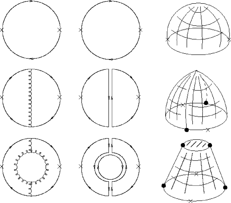
FIG. 2.: Examples of large $N_{c}$ counting for Feynman diagrams. Each row gives three equivalent representations of the same diagram, the first in standard form, the second in double-line notation, and the third as a topological figure. In terms of the quantities in Eqs. (7) and (8), the first diagram has $g_{s}^{0}N_{c}^{1}$, $C=1$, $P=2$, $V=2$, $G=0$, $B=1$; the second has $g_{s}^{2}N_{c}^{2}$, $C=2$, $P=5$, $V=4$, $G=0$, $B=1$; the third has $g_{s}^{4}N_{c}^{3}$, $C=3$, $P=8$, $V=6$, $G=0$, $B=1$. All three scale as $N_{c}^{1}$ and are planar. Crosses indicate current insertions connecting quarks to the QCD vacuum.

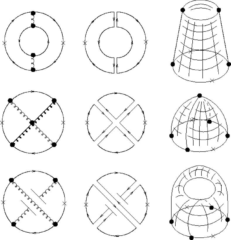
FIG. 3.: More examples of large $N_{c}$ counting for Feynman diagrams. The first line has $g_{s}^{4}N_{c}^{2}$, $C=2$, $P=8$, $V=6$, $G=0$, $B=2$ and scales as $N_{c}^{0}$; the second has $g_{s}^{6}N_{c}^{4}$, $C=4$, $P=10$, $V=7$, $G=0$, $B=1$ and scales as $N_{c}^{1}$; the third has $g_{s}^{4}N_{c}^{1}$, $C=1$, $P=8$, $V=6$, $G=1$, $B=1$, and scales as $N_{c}^{-1}$. Note that only the second diagram is planar and hence leading in $1/N_{c}$.

FIG. 4.: The two distinct types of meson structures equivalent to the QCD three-point function.

FIG. 5.: One leading diagram for glueball-meson mixing.

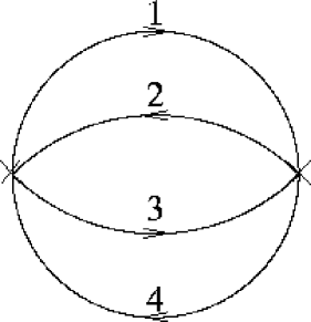
FIG. 6.: Two-point diagram used to study production of multiquark mesons.

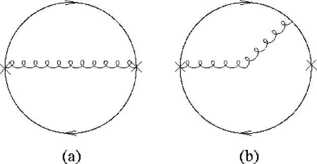
FIG. 7.: Leading two-point diagrams relevant to $(a)$ free hybrid meson propagation, and $(b)$ hybrid-conventional meson mixing.

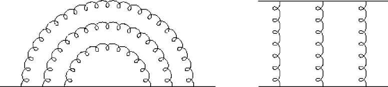
FIG. 8.: Nontrivial “rainbow” and “ladder” diagrams summed by the ’t Hooft model.

FIG. 9.: Full rate for nonleptonic weak decay of meson containing a heavy quark of mass $M$ as a function of $M$. The solid line is computed in the ’t Hooft model and sums over all allowed exclusive modes, while the dashed line is due only to the free heavy quark weak decay diagram.

FIG. 10.: Three sample leading-order connected baryon diagrams contributing to interaction energy. Each square bracket indicates the presence of $N_{c}$ quark lines. Counting combinatoric factors, color loops, and powers of $g_{s}\propto\sqrt{N_{c}}$, one finds that each diagram scales as $N_{c}^{1}$.

FIG. 11.: Simple ladder ($a$) and crossed-ladder ($b$) gluon exchange diagrams for baryons.

FIG. 12.: Sample $1/N_{c}$ leading-order diagrams for baryon-baryon and baryon-meson scattering, respectively. Brackets indicate quarks collected into distinct hadrons.

FIG. 13.: Baryon-pion scattering diagrams used to obtain the amplitude (26), and ultimately, the consistency condition (28).

                        $\,\cdot\cdot\cdot\cdot\cdot\,$                  

=                             $\,\cdot\cdot\cdot\cdot\cdot\,$                                     $\,\cdot\cdot\cdot\cdot\cdot\,$       ,     $J=\frac{1}{2}$

$\oplus$                       $\,\cdot\cdot\cdot\cdot\cdot\,$                                           $\,\cdot\cdot\cdot\cdot\cdot\,$       ,     $J=\frac{3}{2}$

$\cdot$

$\cdot$

$\cdot$

$\oplus$                             $\,\cdot\cdot\cdot\cdot\cdot\,$                   ,     $J=\frac{N_{c}}{2}$

FIG. 14.: The completely symmetric SU($2F$) $N_{c}$-box Young tableau, corresponding to ground-state baryons, decomposed into SU($F$)_flavor $\times$ SU(2)_spin representations.

FIG. 15.: Weight diagram corresponding to the ground-state spin-1/2 representation of SU(3) for $N_{c}>3$. Indicated are the numbers of states at a given site. The longer side has $(N_{c}+1)/2$ sites.

FIG. 16.: Weight diagram corresponding to the ground-state spin-3/2 representation of SU(3) for $N_{c}>3$. Indicated are the numbers of states at a given site. The longer side has $(N_{c}-1)/2$ sites.

FIG. 17.: Experimental values of isospin-averaged mass combinations relative to the common baryon mass, as described in the text (a ratio called experimental accuracy here). Each one corresponds to a particular operator in the $1/N_{c}$ expansion, whose $1/N_{c}$ and SU(3)-breaking suppressions $\epsilon$ label each point.

REFERENCES

- [1] E. Witten, Nucl. Phys. B160 (1979) 57.
- [2] S. Coleman, Aspects of Symmetry (Cambridge University Press, New York) 1985.
- [3] A. V. Manohar, from Probing the Standard Model of Particle Interactions, ed. by F. David and R. Gupta [hep-ph/9802419].
- [4] E. Jenkins, Ann. Rev. Nucl. Part. Sci. 48 (1998) 81.
- [5] G. ’t Hooft, Nucl. Phys. B72 (1974) 461.
-
[6]
O. W. Greenberg, Phys. Rev. Lett. 13 (1964)
598;
M. Y. Han and Y. Nambu, Phys. Rev. 139 (1965) B1006. - [7] N. Cabibbo, G. Parisi, and M. Testa, Nuovo Cim. 4 (1970) 35.
- [8] E852 Collaboration (D. R. Thompson et al., Phys. Rev. Lett. 79 (1997) 1630.
- [9] G. Veneziano, Nucl. Phys. B117 (1976) 519.
- [10] T. D. Cohen, Phys. Lett. B 427 (1998) 348.
- [11] S. Okubo, Phys. Lett. 5 (1963) 165; Phys. Rev. D 16 (1977) 2336; G. Zweig, CERN Report No. 8419 TH 412, 1964 (unpublished), reprinted in Developments in the Quark Theory of Hadrons, ed. by D. B. Lichtenberg and S. P. Rosen (Hadronic Press, Massachusetts, 1980); J. Iizuka, K. Okada, and O. Shito, Prog. Theor. Phys. 35 (1966) 1061; J. Iizuka, Prog. Theor. Phys. Suppl. 37–38 (1966) 21.
- [12] P. Geiger and N. Isgur, Phys. Rev. D 55 (1997) 299.
- [13] G. ’t Hooft, Nucl. Phys. B75 (1974) 461.
- [14] B. Grinstein and R. F. Lebed, Phys. Rev. D 57 (1998) 1366.
-
[15]
T. H. R. Skyrme, Proc. Royal Soc. A 260 (1961)
127;
For a review of the Skyrme model, see
I. Zahed and G. E. Brown, Phys. Rep. 142 (1986) 1;
The initial papers discussing the relation of large baryons and the Skyrme model include
E. Witten, Nucl. Phys. B223 (1983) 422, 433;
G. S. Adkins, C. R. Nappi, and E. Witten, Nucl. Phys. B228 (1983) 552. - [16] J.-L. Gervais and B. Sakita, Phys. Rev. Lett. 52 (1984) 87; Phys. Rev. D 30 (1984) 1795.
-
[17]
F. Gürsey and L. A. Radicati, Phys. Rev. Lett. 13 (1964) 173;
B. Sakita, Phys. Rev. 136 (1964) B1756. - [18] T. Cook and B. Sakita, J. Math. Phys. 8 (1967) 708.
- [19] R. F. Dashen, E. Jenkins, and A. V. Manohar, Phys. Rev. D 49 (1994) 4713.
- [20] E. Jenkins, Phys. Lett. B 315 (1993) 441.
- [21] E. Jenkins and A. V. Manohar, Phys. Lett. B 335 (1994) 452.
- [22] J. L. Goity, Phys. Lett. B 414 (1997) 140.
- [23] D. Pirjol and T.-M. Yan, Phys. Rev. D 57 (1998) 1449 and 5434.
- [24] C.-K. Chow, D. Pirjol, and T.-M. Yan, Cornell U. Report No. CLNS-98-1569 [hep-ph/9807387 ] (unpublished).
- [25] G. Karl and J. E. Paton, Phys. Rev. D 30 (1984) 238.
- [26] A. V. Manohar, Nucl. Phys. B248 (1984) 19.
- [27] C. D. Carone, H. Georgi, and S. T. Osofsky, Phys. Lett. B 322 (1994) 227.
- [28] M. A. Luty and J. March-Russell, Nucl. Phys. B426 (1994) 71.
- [29] R. F. Dashen, E. Jenkins, and A. V. Manohar, Phys. Rev. D 51 (1995) 3697.
- [30] E. Jenkins and R. F. Lebed, Phys. Rev. D 52 (1995) 282.
- [31] M. A. Luty, J. March-Russell, and M. White, Phys. Rev. D 51 (1995) 2332.
- [32] J. Dai, R. F. Dashen, E. Jenkins, and A. V. Manohar, Phys. Rev. D 53 (1996) 273.
- [33] R. Flores-Mendieta, E. Jenkins, and A. V. Manohar, Phys. Rev. D 58 (1998) 094028.
- [34] C. E. Carlson, C. D. Carone, J. L. Goity, and R. F. Lebed, hep-ph/9807334 (to appear in Phys. Lett. B).
- [35] D. B. Kaplan and M. J. Savage, Phys. Lett. B 365 (1996) 244.
- [36] D. B. Kaplan and A. V. Manohar, Phys. Rev. D 56 (1997) 76.
- [37] E. Jenkins, Phys. Rev. D 53 (1996) 2625.
- [38] M. Neubert, Phys. Rep. 245 (1994) 259.
- [39] C.-K. Chow, Phys. Rev. D 54 (1996) 873.
- [40] E. Jenkins, Phys. Rev. D 54 (1996) 4515; 55 (1997) 10.
- [41] R. F. Lebed, Phys. Rev. D 54 (1996) 4463.
- [42] C. D. Carone, H. Georgi, L. Kaplan, and D. Morin, Phys. Rev. D 50 (1994), 5793.
- [43] C. D. Carlson and C. D. Carone, Report No. WM-98-110, hep-ph/9808356 (to appear in Phys. Rev. D); Phys. Rev. D 58 (1998) 053005.
= ,
,
,