Monte-Carlo Study of Bound States in a Few-Nucleon System
– Method of Continued Fractions –

Abstract

The aim of the present paper is to propose a new type of Monte-Carlo method which enables us to study the excited state of many-body systems. It consists of the method of continued fractions (MCF) and a Monte-Carlo random walk for multi-dimensional integration. The convergence of the MCF and its accuracy are studied in detail for a one-dimensional model. As an application of this method to a realistic problem, we study the ground state of ⁴He by using the Volkov potential. It is shown that our results are in good agreement with those of previous works obtained through different types of formalism. This implies that our new method works effectively in the study of many-body nuclear systems.

I Introduction

The exact treatment of nuclear many-body systems is an important benchmark for investigating the dynamics of multi-nucleon systems. It is a testing ground of potential models and equations of motion, such as those involving multi-nucleon interaction, relativistic dynamics, and possible modification of nucleon properties inside nuclei.

At present, various methods to solve many-body problems have been developed. One of the standard methods is the Faddeev or Faddeev-Yakubovsky (FY) equation. The FY equation has been applied to the investigation of the ground state of ⁴He using a realistic nuclear potential.[1, 2] A common problem in attempts to extend the ‘exact’ study of many-body systems is the rapid increase of the number of channels and dimensions as the number of particles increases. One way to overcome this problem is to diagonalize the Hamiltonian in a subspace spanned by appropriate bases chosen using a stochastic method. The other way is the direct calculation of the matrix elements using a Monte-Carlo method. In the Monte-Carlo method, one can perform an effective multi-dimensional integration by taking the importance sampling from the essential part of the phase space.

Extensive works have been carried out by using a variational Monte-Carlo method (VMC)[3] and a Green’s function Monte-Carlo method (GFMC).[4, 5] VMC and GFMC have been applied to the study of the ground state properties of nuclei with mass number $A\leq 7$ using realistic nuclear potential.[5] The bound state energies and also the electro-magnetic properties of few-nucleon systems have been studied extensively. In VMC, we can obtain the upper bound of the ground state energy for which the matrix elements are evaluated by Monte-Carlo integration. Simultaneously, we obtain an analytic form of the trial function which describes the ground state quite well. In GFMC, we start the calculation with a trial function obtained by VMC, and the imaginary-time evolution $e^{-\tau H}$ extracts the improved ground state wave function from the trial function. Here, the imaginary-time evolution is carried out by using the quantum Monte-Carlo random walk method. Due to the $e^{-\tau H}$ projection, we only obtain the properties for the lowest state of the system with a given quantum number. Excited states in the diffusion Monte-Carlo method can be investigated using a diagonalization procedure in the large space shell-model calculation with an auxiliary-field Monte-Carlo approach[6, 7] and in one- and two-dimensional examples of GFMC.[8] For the purpose of conducting systematic studies in few-nucleon systems, it is necessary to investigate excited states as well as the ground state. Therefore we should develop a method for this purpose in the context of few-nucleon physics.

In this paper, we propose a new Monte-Carlo method to study the bound state problems in few-nucleon systems. Here, our purpose is to find an effective method to extract eigenfunctions without referring to the imaginary-time evolution method, but still using the Monte-Carlo random walk. Therefore, the method is not restricted to the ground state problem. We use the method of continued fractions (MCF) as a central formalism in our new calculation method. MCF was originally proposed by J. Horáček and T. Sasakawa [9] as a fast calculational method to evaluate T-matrix elements and was applied to the three-nucleon system. The wave functions which appear in the MCF iteration are generated so as to be orthogonal to the lower order ones. Then the matrix elements calculated by those wave functions rapidly converge. Moreover, this method is simple and allows us to use any function as a starting trial wave function and to adopt a nuclear potential including a many-body potential.

The direct application of MCF with Monte-Carlo integration, however, causes a few serious problems: First, the original form of the MCF iteration formula [10] is not suitable to apply a Monte-Carlo random walk, since the modified Green’s functions used in each iteration are written in a separable form. We find with a slight modification that the iteration formula can be written in a form similar to the diffusion equation. There is, however, a crucial difference between them. In our new iteration formula, a higher order MCF wave function is generated from a lower order one. Therefore, the equation cannot be a simple iteration of the same function as in the diffusion equation. Second, in order to guarantee the orthogonalization of each MCF wave function, we must deal the difference of two MCF wave functions. This causes a sort of the “sign problem”.[11] Here, we propose a correct method of counting the weight in the random walk procedure for an equation of a non-iterative type. As a result, we find out that our method is closely related to “the multiple cancellation” method.[12] With our cancellation method, we can take care of the sign problem in our formula.

The validity of our method of counting weight and the convergence of the MCF are extensively examined for a simple bound state problem in one-dimension including the excited states. As a more realistic example of a multi-dimensional problem, we study $A=4$ nuclei with the Volkov potential.[14] Our method is successful in the treatment both examples.

We briefly review the method of continued fractions in §2. Our random walk method in a non-iterative equation and multiple cancellation mechanism are discussed in §3. We present our results in §4, and a summary is given in §5.

II Method of continued fractions

The method of continued fractions (MCF) has been developed as an efficient method to study scattering problems in atomic and nuclear physics.[9, 10] We briefly review this method, here.

The Schrödinger equation of nuclear bound state can be written as

$$|\phi\rangle=G_{0}(E)V|\phi\rangle\mbox{ ,}$$ (1)

where $G_{0}(E)$ is a free Green’s function,

$$G_{0}(E)=\frac{1}{E-H_{0}}\mbox{ ,}$$ (2)

and $H_{0}$ and $V$ are the kinetic energy of the nucleons and the nuclear potential, respectively.

In this paper, we use the modified Green’s function (MCFG) approach,[9] since it is easy to implement in Monte-Carlo evaluations. We introduce the arbitrary functions $|F_{0}\rangle$ and $|f\rangle$ which are not orthogonal to the eigenfunction $|\phi\rangle$. A new function $|F_{1}\rangle$ is defined as

$$|F_{1}\rangle\equiv G_{0}(E)V|F_{0}\rangle\mbox{ ,}$$ (3)

and a modified Green’s function $G_{1}(E)$ as

$$G_{1}(E)\equiv G_{0}(E)-\frac{|F_{1}\rangle\langle f|}{\langle f|V|F_{0}\rangle}\mbox{ .}$$ (4)

$G_{1}(E)$ is chosen so as to operate only on the space which is orthogonal to $V|F_{0}\rangle$ as

$$G_{1}(E)V|F_{0}\rangle=0\mbox{ .}$$ (5)

We eliminate $G_{0}(E)$ from the Schrödinger equation (1) using (4):

$$|\phi\rangle=\left(G_{1}(E)+\frac{|F_{1}\rangle\langle f|}{\langle f|V|F_{0}\rangle}\right)V|\phi\rangle\mbox{ .}$$ (6)

Then we define $|\phi_{1}\rangle$ as

$$|\phi_{1}\rangle\equiv\frac{1}{1-G_{1}(E)V}|F_{1}\rangle\mbox{ ,}$$ (7)

and (1) can be written as

$$|\phi\rangle=|\phi_{1}\rangle\frac{\langle f|V|\phi\rangle}{\langle f|V|F_{0}\rangle}\mbox{ .}$$ (8)

Multiplying (8) by $\langle f|V$ from the left, we obtain the following condition to determine the bound state energy $E$ and the wave function $|\phi\rangle$:

$$\Omega(E)\equiv\langle f|V|F_{0}\rangle-\langle f|V|\phi_{1}\rangle=0\mbox{ .}$$ (9)

The bound state condition can be written in terms of a continued fraction as

$$|\phi_{i}\rangle\equiv\frac{1}{1-G_{i}(E)V}|F_{i}\rangle\mbox{ ,}$$ (10)

$$|F_{i+1}\rangle=G_{i}(E)V|F_{i}\rangle\mbox{ ,}$$ (11)

and

$$G_{i}(E)=G_{i-1}(E)-\frac{|F_{i}\rangle\langle f|}{\langle f|V|F_{i-1}\rangle}\mbox{ ,}$$ (12)

where $|\phi_{i}\rangle$ is the $i$-th order wave functions. The $i$-th Green’s function $G_{i}(E)$ satisfies the orthogonality relation

$$G_{i}(E)V|F_{j}\rangle=0\mbox{ .}\hskip 11.38109pt(i=j+1)$$ (13)

We rewrite (10) using (12), multiply $\langle f|V$ from the left, and obtain the following iteration formula for $|\phi_{i}\rangle$:

$$\langle f|V|\phi_{i}\rangle=\frac{\langle f|V|F_{i}\rangle^{2}}{\langle f|V|F_{i}\rangle-\langle f|V|\phi_{i+1}\rangle}\mbox{ .}$$ (14)

As a result, the bound state condition (9) can be written in the form of a continued fraction:

$$\Omega(E)=x_{0}-\frac{x_{1}^{2}}{\displaystyle{x_{1}-\frac{x_{2}^{2}}{\displaystyle{x_{2}-\frac{x_{3}^{2}}{\displaystyle{x_{3}{}-\,_{\ddots}}}}}}}\mbox{ .}$$ (15)

Here, the matrix elements $x_{i}$ are defined as

$$x_{i}\equiv\langle f|V|F_{i}\rangle\mbox{ .}$$ (16)

In the MCF calculation, we only need to generate $|F_{i}\rangle$ and $G_{i}(E)$ iteratively, following the iteration procedure (11) and (12). In this procedure, $G_{i}(E)$ projects out the states which are orthogonal to the lower order wave functions, as indicated in (13). Therefore, $x_{i}$ is expected to become smaller for larger $i$, and rapidly converges into zero. The advantage of this continued fraction series based on Ref. [10] for the Monte-Carlo calculation is that the $x_{i}$ are simply given by the matrix element of the potential between $|F_{i}\rangle$ and the analytically known function $|f\rangle$, in contrast to those given in Ref. [9], where we need the matrix elements between $|F_{i}\rangle$.

The bound state energy is determined by solving the equation

$$\Omega(E)=0$$ (17)

numerically. In actual practice, we perform a parameter search for $E$. Since we do not adopt any projections onto the ground state, we can also apply MCF to study the excited states without any restriction such as the $e^{-\tau H}$ projection.

Once the energy of the bound state has been determined, the relevant eigenfunction is given as

$$|\phi\rangle={\cal N}\left[\,|F_{1}\rangle+y_{1}|F_{2}\rangle+y_{1}y_{2}|F_{3}\rangle+y_{1}y_{2}y_{3}|F_{4}\rangle+\cdots\right]\mbox{ ,}$$ (18)

where $y_{i}$ is defined as

$$y_{i}\equiv\frac{x_{i}}{x_{i}-\langle f|V|\phi_{i+1}\rangle}\mbox{ ,}$$ (19)

and ${\cal N}$ is a normalization constant.

III Continued fractions and Monte-Carlo method

The original form of the MCF iteration formula (11) is not suitable for Monte-Carlo evaluations. The difficulty is caused by the Green’s functions $G_{i}(E)$. Since the $G_{i}(E)$ obey the iteration formula (12) and are of a separable form,

$$G_{i}(E)=G_{i-1}(E)-\frac{|F_{i}\rangle\langle f|}{x_{i-1}}\mbox{ ,}$$ (20)

it does not seem practical to generate the random numbers according to the probability of $G_{i}(E)$. In order to resolve these problems, we use the orthogonality relation (13) and modify the iteration formula (11) as follows:

$$|F_{i+1}\rangle=G_{0}(E)V\left[|F_{i}\rangle-|F_{i-1}\rangle\frac{x_{i}}{x_{i-1}}\right]\mbox{ .}$$ (21)

The advantage of this formula is that a higher order wave function $|F_{i+1}\rangle$ is always generated by the free Green’s function $G_{0}(E)$, which has a simple analytical form. Therefore, we can use the Monte-Carlo random walk technique in the MCF iteration procedure.

However, it should be noted that the iteration formula (21) is not of the same form as the original Schrödinger equation. The Schrödinger equation,

$$|\phi\rangle=G_{0}(E)V|\phi\rangle\mbox{ ,}$$ (22)

can be regarded as a diffusion equation. $|\phi\rangle$ will converge to a ground state by iterating (22) with a Monte-Carlo random walk. In contrast, (21) can be written as

$$|\psi_{1}\rangle=G_{0}(E)V|\psi_{0}\rangle\mbox{ ,}$$ (23)

where $|\psi_{1}\rangle$ and $|\psi_{0}\rangle$ represent $|F_{i+1}\rangle$ and $[|F_{i}\rangle-|F_{i-1}\rangle x_{i}/x_{i-1}]$, respectively. In our iteration formula (23), the wave function $|\psi_{1}\rangle$ has different functional form from $|\psi_{0}\rangle$ and is generated from the two terms $|F_{i}\rangle$ and $|F_{i-1}\rangle$. Therefore, we cannot naively apply the random walk technique of the diffusion equation. Otherwise, a destructive interference of $|F_{i}\rangle$ and $|F_{i-1}\rangle$ in (21) may cause the “sign problem”.

In this section, we extend the random walk technique for (23) and propose a new method of counting weight. The destructive interference of two terms in (21) can be taken care of by our proper method of counting weight.

A Random walk in MCF

We study an algorithm to apply the random walk method with the free Green’s function $G_{0}(R,R^{\prime})$ to our following iteration formula of MCF:

$$\psi_{1}(R)=\int G_{0}(R,R^{\prime})W(R^{\prime})\psi_{0}(R^{\prime})dR^{\prime}\mbox{ .}$$ (24)

Here we re-scale the variables so that the free Green’s function $G_{0}(R,R^{\prime})$ is normalized as

$$\left[-\nabla^{2}_{R}+1\right]G_{0}(R,R^{\prime})=\delta(R-R^{\prime})\mbox{ ,}$$ (25)

where $R$ denotes an $M$-dimensional vector, i.e. $R=\{z_{1},\cdots,z_{M}\}$ defined in the standard manner given in Ref. [13]. The potential $W(R)$ is defined as

$$W(R)\equiv-V(R)/B\mbox{ ,}$$ (26)

where $B$ is the binding energy.

For simplicity, we assume that the wave functions $\psi_{1}(R)$ and $\psi_{0}(R)$ and the potential $W(R)$ are positive definite. Note that the positive sign of $W(R)$ implies that this is an attractive potential. We assume $\psi_{1}(R)$ and $W(R)\psi_{0}(R)$ are represented by the sum of points $\{R_{k,i}\}$ distributed with the probability $\psi_{k}(R)$ and the weights $\{W_{k,i}\}$, where $k=0,1$. The question is how $\{R_{1,j}\}$ and $\{W_{1,j}\}$ should be generated from given sets of $\{R_{0,j}\}$ and $\{W_{0,j}\}$. The relation can be obtained by studying the following overlap integral of $\psi_{1}(R)$ with an arbitrary function $F(R)$:

$${\cal I}=\int F(R)\psi_{1}(R)dR\mbox{ .}$$ (27)

${\cal I}$ is given by using $\{R_{1,j}\}$ and $\{W_{1,j}\}$ as

$${\cal I}=\sum_{j}^{N}W_{1,j}F(R_{1,j})\mbox{ ,}$$ (28)

while the same integral is expressed by $\{R_{0,j}\}$ and $\{W_{0,j}\}$ using (24) as

$${\cal I}=\int F(R)\sum_{i}^{N}W_{0,i}G_{0}(R,R_{0,i})dR\mbox{ ,}$$ (29)

where $N$ is the number of sampling points.

We multiply the integrand of (29) by unity in the form $G_{0}(R,X)/G_{0}(R,X)$ and obtain

$${\cal I}=\int A(R,X)G_{0}(R,X)dR\mbox{ ,}$$ (30)

where $A(R,X)$ is defined as

$$A(R,X)\equiv F(R)\sum_{i}^{N}W_{0,i}\frac{G_{0}(R,R_{0,i})}{G_{0}(R,X)}\mbox{ .}$$ (31)

Here, $X$ can be an arbitrary vector in $M$-dimensional space. We impose hyper spherical boundary conditions on $G_{0}(R,X)$ for the bound state problem,

$$G_{0}(R,X)=0\hskip 8.53581pt\mbox{for}\hskip 8.53581pt|R|,|X|\rightarrow\infty\mbox{.}$$ (32)

$G_{0}(R,X)$ becomes a function of distance $|{\cal R}|$, where ${\cal R}$ is defined as ${\cal R}\equiv R-X$. Since $G_{0}(R,X)$ is normalized as

$$\int G_{0}(R,X)dR=\int G_{0}(|{\cal R}|)d{\cal R}=1\mbox{ ,}$$ (33)

$G_{0}(|{\cal R}|)$ can be regarded as a probability function.

We change the integral variable from $R$ to ${\cal R}$ in (30) and generate a set of random numbers $\{{\cal R}_{j}\}$ with probability $G_{0}(|{\cal R}|)$. The algorithm to generate $\{{\cal R}_{j}\}$ in $M$ dimensional space is given in Ref. [13]. Equation (30) is rewritten as follows:

$${\cal I}=\sum_{j}^{N}F(X+{\cal R}_{j})\frac{\sum_{i}W_{0,i}G_{0}(X+{\cal R}_{j},R_{0,i})}{NG_{0}(X+{\cal R}_{j},X)}\mbox{ .}$$ (34)

Since (34) holds for any values of $X$, we choose $X$ as $R_{0,j}$ for the $j$-th random number ${\cal R}_{j}$. Comparing (34) with (28), we can define the new points $R_{1,j}$ and the weight $W_{1,j}$ as

$$R_{1,j}\equiv R_{0,j}+{\cal R}_{j}\mbox{ ,}$$ (35)

and

$$W_{1,j}\equiv\frac{\sum_{i}W_{0,i}G_{0}(R_{0,j}+{\cal R}_{j},R_{0,i})}{NG_{0}(R_{0,j}+{\cal R}_{j},R_{0,j})}\mbox{.}$$ (36)

As a result, (35) and (36) show how the distribution of points $\{R_{1,j}\}$ and the weights $\{W_{1,j}\}$ of $\psi_{1}(R)$ should be generated from those of $W(R)\psi_{0}(R)$. A new point $R_{1,j}$ is generated by a random walk from $R_{0,j}$ similar to the diffusion equation. However, a new weight $W_{1,i}$ is generated by taking into account all of the old points $\{R_{0,i}\}$ and weights $\{W_{0,i}\}$ through the free Green’s function. In the naive random walk method, $W_{1,j}$ is simply given by $W_{0,i}$, which projects into the ground state wave function. For a non-diffusion type integral formula like (24), weights of new points should be generated by using this method of counting weight.

B Multiple cancellation

In general, $\psi_{0}(R)$ and $W(R)$ are not positive definite, and we must include their sign information in our formula. This can be done by adding the sign $s_{0,j}$ to the weight $W_{0,j}$ as

$$W_{0,j}\Rightarrow s_{0,j}W_{0,j}\mbox{ .}$$ (37)

Similarly, adding the sign $s_{1,j}$ to $W_{1,j}$, (36) is replaced by

$$s_{1,j}W_{1,j}=\frac{\sum_{i}s_{0,i}W_{0,i}G_{0}(R_{0,j}+{\cal R}_{j},R_{0,i})}{NG_{0}(R_{0,j}+{\cal R}_{j},R_{0,j})}\mbox{ .}$$ (38)

Equation (38) is quite similar to the “multiple cancellation” method proposed by J. B. Anderson et al..[12] The multiple cancellation method with a random walk has been applied to atomic physics, where it has provided very accurate results. In the conventional random walk technique, points with positive and negative signs walk independently. Then the weight of each point grows, and a destructive interference of these wave functions induces large numerical errors. On the other hand, our formula (38) shows that weight and sign of new points are generated by taking into account all the weights and signs of old points. Therefore, the points with positive and negative weights are canceled out in the course of counting the new weight. Equation (38) plays an essential role in the MCF calculation, and its importance will be demonstrated in the one-dimensional example given in the next section.

IV Applications to bound state problems

The procedure of our method is summarized as follows:

1. Assume an appropriate form of the trial function $|F_{0}\rangle$.

2. Distribute the points by the Metropolis method[15] according to the functional form of $|F_{0}\rangle$.

3. Calculate the matrix element $x_{i}$ of the $i$-th iteration step.

4. Generate new points of $|F_{i+1}\rangle$ by a random walk according to the procedure described in the previous section.

5. Iterate steps 3 and 4 until the $x_{i}$ and $\Omega(E)$ converge.

The binding energy $B(=-E)$ is determined by searching for an energy that satisfies the condition $\Omega(E)=0$.

A One-dimensional model

As a simplest example, we study a one-dimensional potential model. In this one-dimensional problem, we can study the validity of our method by comparing with a conventional numerical method. We take the mass of the particle as $m=940$ MeV and a simple central potential $V(x)$ of exponential form with a one pion range as follows:

$$V(x)=V_{0}\exp(-a|x|)$$ (39)

with

$$V_{0}=-69.3\hskip 2.84526pt(\mbox{MeV})\mbox{ , }a=0.711\hskip 2.84526pt(\mbox{fm}^{-1})\mbox{ .}$$ (40)

The strength of the potential is chosen so as to produce three bound states at $-$38.7, $-$10.6 and $-$2.01 MeV. The binding energy of the second excited state is small, and is compared to the deuteron binding energy. Since this model is one-dimensional and does not contain any other degrees of freedom, such as spin or isospin, the wave function of the bound states can be classified by their parity. The ground and second excited states are even parity states, and the first excited state is an odd parity state. The validity of our method for the second excited state is particularly interesting, since it has the same symmetry as the ground state.

Introducing a dimensionless variable $z$ defined as

$$z=\sqrt{2mB}x\mbox{ ,}$$ (41)

the free Green’s function is given by

$$G_{0}(z,z^{\prime})=\frac{1}{2}\exp(-|z-z^{\prime}|)\mbox{.}$$ (42)

The trial function is taken to be a Gaussian form as follows:

$$|F_{0}\rangle=|f\rangle = \frac{1}{\sqrt{b\sqrt{\pi}}}\exp(-\frac{x^{2}}{2b^{2}})\hskip 2.84526pt\mbox{ for even parity,}$$ (43)

$$= \sqrt{\frac{2}{b\sqrt{\pi}}}\frac{x}{b}\exp(-\frac{x^{2}}{2b^{2}})\hskip 2.84526pt\mbox{ for odd parity.}$$ (44)

We assume $b=3$ (fm) for the ground and first excited states and $b=10$ (fm) for the second excited state.

In the Monte-Carlo calculation, the numbers of sampling points were 20,000, 70,000 and 100,000 for the ground, first, and second excited states, respectively. We needed a larger number of points for the excited states than for the ground state in order to obtain reasonable accuracy. The initial distribution of points with the probability $||F_{0}\rangle|$ was generated by the Metropolis method. A typical number for the thermalization step was $100$ in this problem.

The fast convergence of the MCF iteration is related to the orthogonality relation in (13), which is implemented in our iteration formula in (21). As an example, we consider the second order MCF wave function $|F_{2}\rangle$,

$$|F_{2}\rangle=G_{0}(E)V\left[|F_{1}\rangle-|F_{0}\rangle\frac{x_{1}}{x_{0}}\right]\mbox{ .}$$ (45)

$|F_{2}\rangle$ is generated by two terms, $|F_{1}\rangle$ and $-|F_{0}\rangle x_{1}/x_{0}$, which will cancel each other. The higher order $|F_{i}\rangle$ decreases quickly with this cancellation mechanism. Therefore, accurate treatment of this cancellation is important. If we generate $|F_{2}\rangle$ from two terms independently, the resultant distribution of the points for $|F_{2}\rangle$ is given by the large overlap of the points with positive and negative signs shown in Fig. 1 at the energy of the second excited state. $|F_{2}\rangle$ generated from these points will include large errors, which is just our “sign problem”. Because of this sign problem, it is difficult to obtain convergence for the higher order MCF wave functions in the standard random walk method. On the other hand, using our method of counting weight in (38), the cancellation between two terms is performed analytically, and the distribution of the positive points for $|F_{2}\rangle$ is clearly separated from the negative points, as shown in Fig. 2. Our method of counting weight plays an important role in MCF iteration with the Monte-Carlo method.

MCF wave functions at each iteration step are shown in Fig. 3. They decrease rapidly as the iteration steps increase, even for the second excited state. This agrees well with the results obtained using the standard method of numerical integration.

Consequently, the matrix elements $x_{i}$ defined in (16) and $\Omega(E)$ also converge rapidly as a function of the iteration step as shown in Fig. 4 and 5, respectively. A few steps of iteration is enough to obtain reasonable convergence for the ground and first excited states. Slower convergence for the second excited state is due to our simple Gaussian trial function, even though one expects nodes in the wave function of the second excited state.

The energy dependence of $\Omega(E)$ is shown in Fig. 6 for the ground state. To determine the binding energy from the condition $\Omega(E)=0$, we fitted $\Omega(E)$ by using the linear energy-dependence of $\Omega(E)=0$ near the binding energy with the least square search method. Since values of $\Omega(E)$ fluctuate due to sampling errors, we performed calculations several times with different sets of random numbers. Averaging these results, we obtained the energies of three bound states and errors estimated by the standard deviation, as shown in Table I. Our results with the Monte-Carlo method are in a good agreement with those of the ‘exact’ calculation for all three states.

Once we obtained the binding energies, the eigenfunctions were given by the MCF wave functions $|F_{i}\rangle$ and matrix elements $x_{i}$. The wave functions for the ground, first, and second excited states are shown in Fig. 7. The wave functions are also in good agreement with the ‘exact’ calculation. Note that we started with a trial function without nodes for the second excited state. We could use more realistic trial functions with nodes, and if we did so we would obtain faster convergence. However, our result shows that it is not necessary to know the correct nodes of the wave function when we construct a trial function in this method. In summary, our new Monte-Carlo method works for the calculation of binding energies and wave functions including the excited states, and we believe that our method will be useful in studying few-nucleon bound state systems.

B Four-nucleon bound state as an example of a multi-dimensional problem

As a realistic example, we study a four-nucleon bound state in three-dimensional space. The Schrödinger equation is expressed as follows:

$$-\sum_{k=1}^{3}\frac{1}{2\mu_{k}}\nabla_{r_{k}}^{2}|\phi\rangle+\sum_{i<j}^{4}V_{ij}|\phi\rangle=-B|\phi\rangle\mbox{ .}$$ (46)

Here, the $r$_k are the Jacobi coordinates defined as

$\displaystyle\left\{\begin{array}[]{lcl}\mbox{\boldmath$r$}_{1}&=&\mbox{\boldmath$x$}_{2}-\mbox{\boldmath$x$}_{1}\mbox{ ,}\\ \mbox{\boldmath$r$}_{2}&=&\mbox{\boldmath$x$}_{3}-(\mbox{\boldmath$x$}_{1}+\mbox{\boldmath$x$}_{2})/2\mbox{ ,}\\ \mbox{\boldmath$r$}_{3}&=&\mbox{\boldmath$x$}_{4}-(\mbox{\boldmath$x$}_{1}+\mbox{\boldmath$x$}_{2}+\mbox{\boldmath$x$}_{3})/3\mbox{ ,}\end{array}\right.$and the $\mu_{k}$ are reduced masses corresponding to the coordinates $\mbox{\boldmath$r$}_{k}$:

$\displaystyle\left\{\begin{array}[]{lcl}\mu_{1}&=&m/2\mbox{ ,}\\ \mu_{2}&=&2m/3\mbox{ ,}\\ \mu_{3}&=&3m/4\mbox{ .}\end{array}\right.$

Here, we adopt the Volkov potential, which is a central potential and has a soft core at short range:[14]

$$V_{ij}=V_{1}\exp(-a_{1}r_{ij}^{2})+V_{2}\exp(-a_{2}r_{ij}^{2})\mbox{ ,}$$ (47)

with

$\displaystyle\left\{\begin{array}[]{ll}V_{1}=-83.34\mbox{ (MeV) ,}&a_{1}=1.60^{-2}\mbox{ (fm${}^{-2}$) ,}\\ V_{2}=144.86\mbox{ (MeV) ,}&a_{2}=0.82^{-2}\mbox{ (fm${}^{-2}$) ,}\mbox{ .}\end{array}\right.$Since the ground state energy of ⁴He using this potential has been studied by various methods such as the Faddeev-Yakubovsky (FY) method taking into account only the $S$-wave component,[1] the stochastic variational method (SVM)[16] and the hyperspherical harmonics (HH),[17] it is a good example to examine our method in a four-body system.

The free Green’s function in dimensionless coordinates is expressed as

$$G_{0}(R,R^{\prime})=\frac{1}{2(2\pi)^{4}}\frac{1}{{\cal R}^{4}}\left(1+\frac{6}{{\cal R}}+\frac{15}{{\cal R}^{2}}+\frac{15}{{\cal R}^{3}}\right)\exp(-{\cal R})\mbox{ ,}$$ (48)

where ${\cal R}\equiv|R-R^{\prime}|$ is a relative distance in the nine-dimensional space. As the dimensionality increases, the free Green’s function becomes more singular at ${\cal R}=0$. It is rather difficult to treat the singularity of the free Green’s function with the conventional integration method. Since the random walk method inverts the free Green’s function analytically, we can obtain numerically stable results. A standard method to generate points with the probability $G_{0}({\cal R})$ is given in Ref. [13].

The ground state of ⁴He is expected to be spatially symmetric and anti-symmetric in spin-isospin space. Then we take a trial function $|F_{0}\rangle$ given by the product of a Gaussian wave function $|\varphi_{s}\rangle$, a correlation function $g(r)$ and the spin-isospin function $|\Xi\rangle$, as

$$|F_{0}\rangle={\cal N}\prod_{i<j}g(r_{ij})|\varphi_{s}\rangle|\Xi\rangle\mbox{ ,}\\$$ (49)

with

$$|\varphi_{s}\rangle=\prod_{i<j}\exp(-r_{ij}^{2}/2b_{0}^{2})\mbox{ ,}$$ (50)

where $b_{0}$ is a size parameter. We used the form of correlation function $g(r)$

$$g(r_{ij})=[1-\alpha\exp(-r_{ij}^{2}/b_{g})]^{2}$$ (51)

with

$\displaystyle\alpha=0.11\mbox{ , }b_{g}=0.5\mbox{ (fm${}^{2}$)}\mbox{ .}$The parameters of the correlation function are determined to simulate the wave function of a two-nucleon bound state in this potential. The size parameter $b_{0}$ of the Gaussian wave function in (50) is simply determined by the variational method with one parameter. For the trial function $|f\rangle$, we assume the same functional form as $|F_{i}\rangle$, and take a slightly larger value of the size parameter $b_{0}$,

$$b_{0} = 3.0\mbox{ (fm) : for }|F_{0}\rangle$$ (52)

$$= 4.5\mbox{ (fm) : for }|f\rangle\mbox{ .}$$ (53)

Since the Volkov potential is a central potential with no exchange terms, the symmetry of the spatial and spin-isospin wave functions are preserved separately.

The convergence of $x_{i}$ is displayed in Fig. 8, which shows that three-times iterations are enough in this example. Similarly, $\Omega(E)$ also converges rapidly, as shown in Fig. 9. Here, we take $N=200,000$ sampling points.

The bound state energy and its uncertainty are estimated in the same way as in the one-dimensional case. We assume a linear function for fitting the energy dependence of $\Omega(E)$, as shown in Fig. 10. As a result, we obtain $E=-29.88\pm 0.59$ (MeV). Our results for the binding energy of ⁴He are in good agreement with the results of the other methods within uncertainties, as tabulated in Table II. It is shown that our method also works for higher dimensional examples.

V Summary and discussion

The Monte-Carlo method is useful in the study of the bound state of the many-nucleon systems because of its simplicity and efficiency for multi-dimensional calculations. In this work, we propose a new method to study the bound state of a few-nucleon system without using the diffusive-type projection method. Therefore it is expected to work not only for the ground state but also for excited states.

We used the method of continued fractions (MCF) as the main formalism of the calculation. The advantages of this method are its ability to calculate the excited states and the rapid convergence of the continued fraction series. We modified the original formula of MCF into a suitable form for the Monte-Carlo random walk method. We generated MCF wave functions by the random walk method. Here, it was shown that the cancellation mechanism of lower order MCF wave functions is important, and we should use our method of counting weight in this calculation to avoid the “sign problem”.

Our method was examined in application to a one-dimensional problem in detail. We demonstrated that our new method works even for the calculation of excited states. We also studied the bound state of a four-nucleon system and obtained results that compare well with those of other methods. These facts suggest that our method is a powerful method to study the bound states of few-nucleon systems.

Application of this method to few-nucleon systems with realistic nuclear potentials including exchange terms is one of our future problems. Here, we have to deal with the coupled channel problem of wave functions with various types of exchange symmetry. It is important to retain the correct symmetry of the wave function in each iteration step. It is also necessary to take into account the correlation of nucleons in the trial function as much as possible. The wave function obtained by a fully variational calculation should be used as a more plausible trial function in our procedure. This will also accelerate the convergence of the continued fraction series.

FIG. 1.: MCF wave functions at energy (2.01 MeV) of the 2nd-excited state. The solid line, dotted line, and dashed line correspond to $|F_{2}\rangle$, $|F_{1}\rangle$, and $-|F_{0}\rangle x_{1}/x_{0}$, respectively.

FIG. 2.: MCF wave function $|F_{2}\rangle$ generated by our method of weight counting. The solid and dotted lines correspond to the population of the points for positive and negative weight, respectively.

FIG. 3.: The wave function of MCF, $|F_{i}\rangle$, at the energy of the 2nd-excited state ($-2.01$ MeV). The solid lines are obtained by Monte-Carlo method, and the dashed lines are obtained by a numerically ‘exact’ method. The numbers $(0\sim 5)$ specify the wave functions $|F_{i}\rangle$. Normalization of the wave functions obtained by the Monte-Carlo method is adjusted to the ‘exact’ ones.

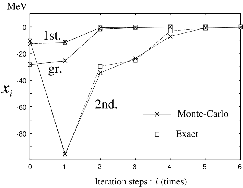
FIG. 4.: Convergence of $x_{i}$ as a function of the iteration step $i$ for the ground, 1st-, and 2nd-excited states in units of MeV. Cross points were obtained by the Monte-Carlo method, while the box points were obtained by a numerically ’exact’ method.

FIG. 5.: Convergence of $\Omega(E)$ as a function of the iteration step $i$ at the ground state energy with arbitrary scale. The points marked by crosses and boxes were obtained by the Monte-Carlo method and a numerically ‘exact’ methods, respectively.

FIG. 6.: Energy dependence of $\Omega(E)$. Points marked by crosses were obtained by the Monte-Carlo method. The dotted-dashed line was obtained by a least square fitting. The units of the vertical axis are the same as in Fig. 5.

FIG. 7.: The eigenfunction for the ground, 1st-, and 2nd-excited states. The solid lines were obtained by the Monte-Carlo method. The dashed lines were obtained by a numerically ‘exact’ method. Normalization of the wave functions obtained by the Monte-Carlo method were adjusted to the exact ones.

FIG. 8.: Convergence of $x_{i}$ as a function of the iteration step $i$ at $B=30$ (MeV).

FIG. 9.: Convergence of $\Omega(E)$ as a function of the iteration step $i$ at $B=$30 (MeV).

FIG. 10.: Energy dependence of $\Omega(E)$, fitted using the same method as in the one-dimensional model.

state	‘exact’	Monte-Carlo
ground	$-38.7$	$-38.8$ $\pm$ 0.1
1st-excited	$-10.6$	$-10.6$ $\pm$ 0.1
2nd-excited	$-2.01$	$-2.03$ $\pm$ 0.14

TABLE I.: The eigenvalues (MeV) for the ground, 1st-, and 2nd-excited states. The results obtained by the Monte-Carlo method are compared with those obtained by a numerically ‘exact’ method.

Method	Energy (MeV)
Faddeev-Yakubovsky [1]	$-30.27$
HH [17]	$-30.40$
SVM [16]	$-30.42$
MCF with MC	$-29.88$ $\pm$ 0.59

TABLE II.: The bound state energy of ⁴He.

REFERENCES

- [1] H. Kamada and W. Glöckle, Nucl. Phys. A548 (1992) 205.
- [2] W. Glöckle and H. Kamada, Phys. Rev. Lett. 71 (1993) 971.
- [3] J. Carlson, V. R. Pandharipande and R. B. Wiringa, Nucl. Phys. A401 (1983) 59.
- [4] J. Carlson, Phys. Rev. C36 (1987) 2026; C38 (1988) 1879.
- [5] B. S. Pudliner, V. R. Pandharipande, J. Carlson, S. C. Pieper and R. B. Wiringa, Phys. Rev. C56 (1997) 1720.
- [6] M. Honma, T Mizusaki and T. Otsuka, Phys. Rev. Lett. 75 (1995) 1284; 77 (1996) 3315.
- [7] K. Kume, K. Sato and Y. Umemoto, Phys. Rev. C55 (1997) 2866.
- [8] T. Cheon, Prog. Theor. Phys. 96 (1996) 971.
- [9] J. Horáček and T. Sasakawa, Phys. Rev. A28 (1983) 2151; A30 (1984) 2274; C32 (1985) 70.
- [10] T. Sasakawa and S. Ishikawa, Few-Body Syst. 1 (1986), 3.
- [11] D. M. Arnow, M. H. Kalos, M. A. Lee and K. E. Schmidt J. Chem. Phys. 77 (1982), 5562.
- [12] J. B. Anderson, C. A. Traynor and B. M. Boghosian, J. Chem. Phys. 95 (1991), 7418.
- [13] M. H. Kalos, Phys. Rev. 128 (1962) 1791.
- [14] A. B. Volkov, Nucl. Phys. 74 (1965) 33.
- [15] N. Metropolis, A. W. Rosenbluth, M. N. Rosenbluth, A. H. Teller and E. Teller, J. Chem. Phys. 21 (1953), 1087.
- [16] K. Varga and Y. Suzuki, Phys. Rev. C52 (1995) 2885.
- [17] J. L. Ballot, Z. Phys. A302 (1981), 347.