Fluid Dynamics for Relativistic Nuclear Collisions

Abstract

I give an introduction to the basic concepts of fluid dynamics as applied to the dynamical description of relativistic nuclear collisions.

1 Introduction and Conclusions

Modelling the dynamic evolution of nuclear collisions in terms of fluid dynamics has a long-standing tradition in heavy-ion physics, for a review see [1, 2, 3]. One of the main reasons is that one essentially does not need more information to solve the equations of motion of ideal fluid dynamics than the equilibrium equation of state of matter under consideration. Once the equation of state is known (and an initial condition is specified), the equations of motion uniquely determine the dynamics of the collision. Knowledge about microscopic reaction processes is not required. This becomes especially important when one wants to study the transition from hadron to quark and gluon degrees of freedom, as predicted by lattice simulations of quantum chromodynamics (QCD) [4]. The complicated deconfinement or hadronization processes need not be known in microscopic detail, all that is necessary is the thermodynamic equation of state as computed by e.g. lattice QCD. This fact has renewed interest in fluid dynamics to study the effects of the deconfinement and chiral symmetry restoration transition on the dynamics of relativistic nuclear collisions. Such collisions are presently under intense experimental investigation at CERN’s SPS and Brookhaven National Laboratory’s AGS and (beginning Fall 1999) RHIC accelerators.

In this set of lectures I give an overview over the basic concepts and notions of relativistic fluid dynamics as applied to the physics of heavy-ion collisions. The aim is not to present a detailed and complete review of this field, but to provide a foundation to understand the literature on current research activities in this field. This has the consequence that the list of references is far from complete, that I will not make any attempt to compare to actual experimental data, and that some interesting, but more applied topics (such as transverse collective flow) will not be discussed here. In Section 2, I discuss the basic concepts of relativistic fluid dynamics. First, I present a derivation of the fluid-dynamical equations of motion. A priori, there are more unknown functions than there are equations, and one has to devise approximation schemes in order to close the set of equations of motion. The most simple is the ideal fluid approximation, which simply discards some of the unknown functions. Another one is the assumption of small deviations from local thermodynamical equilibrium, which leads to the equations of dissipative fluid dynamics. A brief discussion of multi-fluid models concludes this section. In Section 3 I discuss numerical aspects of solution schemes for ideal relativistic fluid dynamics. Section 4 is devoted to a discussion of one-dimensional solutions of ideal fluid dynamics. After presenting a classification of possible wave patterns in one spatial dimension, for both thermodynamicall normal as well as anomalous matter, I discuss the expansion of semi-infinite matter into vacuum. This naturally leads to the discussion of the Landau model for the one-dimensional expansion of a finite slab of matter. The Landau model is historically the first fluid-dynamical model for relativistic nuclear collisions. However, more realistic is, at least for ultrarelativistic collision energies, the so-called the Bjorken model which is subsequently presented. The main result of this section is the time delay in the expansion of the system due to the softening of the equation of state in a phase transition region. This may have potential experimental consequences for nuclear collisions at RHIC energies, where one wants to study the transition from hadron to quark and gluon degrees of freedom. Finally, Section 5 concludes this set of lectures with a discussion on how to decouple particles from the fluid evolution in the so-called “freeze-out” process and compute experimentally observable quantities like single inclusive particle spectra.

Units are $\hbar=c=k_{\rm B}=1$. The metric tensor is $g^{\mu\nu}=\mbox{diag}(+,-,-,-)$. Upper greek indices are contravariant, lower greek indices covariant. The scalar product of two 4-vectors $a^{\mu}\,,\,\,b^{\mu}$ is denoted by $a^{\mu}\,g_{\mu\nu}\,b^{\nu}\equiv a^{\mu}\,b_{\mu}\equiv a\cdot b$. The latter notation is also used for the scalar product of two 3-vectors $\vec{a},\,\vec{b}$, $\vec{a}\cdot\vec{b}$.

2 The Basics

In this section, I first derive the conservation equations of relativistic fluid dynamics. If there are $n$ conserved charges in the fluid, there are $4+n$ conservation equations: 1 for the conservation of energy, 3 for the conservation of 3-momentum, and $n$ for the conservation of the respective charges. In the general case, however, there are $10+4\,n$ independent variables: the 10 independent components of the energy-momentum tensor (which is a symmetric tensor of rank 2), and the 4 independent components of the 4-vectors of the $n$ charge currents. Thus, the system of fluid-dynamical equations is not closed, and one requires an approximation in order to solve it.

The simplest approximation is the ideal fluid assumption which reduces the number of unknown functions to $5+n$. The equation of state of the fluid then provides the final equation to close the system of conservation equations and to solve it uniquely. Another approximation is the assumption of small deviations from an ideal fluid and leads to the equations of dissipative fluid dynamics. In this approximation one provides an additional set of $6+3\,n$ equations to close the set of equations of motion. Finally, I also briefly discuss multi-fluid-dynamical models.

2.1 The Conservation Equations

Fluid dynamics is equivalent to the conservation of energy, momentum, and net charge number. Consider a single fluid characterized locally in space-time by its energy-momentum tensor $T^{\mu\nu}(x)$ and by the $n$ conserved net charge currents $N^{\mu}_{i}(x)\,,\,i=1,\ldots,n$. (Conserved charges are for example the electric charge, baryon number, strangeness, charm, etc.) Consider now an arbitrary hypersurface $\Sigma$ in 4-dimensional space-time. The tangent 4-vector on this surface is $\Sigma^{\mu}(x)$. The normal vector on a surface element $\D\Sigma$ of $\Sigma$ is denoted by $\D\Sigma_{\mu}(x)$. By definition, $\D\Sigma\cdot\Sigma=0$. The amount of net charge of type $i$ and of energy and momentum flowing through the surface element $\D\Sigma$ is given by

$$\D N_{i} \equiv \D\Sigma\cdot N_{i}\,\,,\,\,\,i=1,\ldots,n\enspace,$$ (1)

$$\D P^{\mu} \equiv \D\Sigma_{\nu}\,T^{\mu\nu}\,\,,\,\,\,\mu=0,\ldots,3\enspace.$$ (2)

Now consider an arbitrary space-time volume $V_{4}$ with a closed surface $\Sigma$. If there are neither sources nor sinks of net charge and energy-momentum inside $\Sigma$, one has

$$\oint_{\Sigma}\D\Sigma\cdot N_{i} \equiv 0\,\,,\,\,\,i=1,\ldots,n\enspace,$$ (3)

$$\oint_{\Sigma}\D\Sigma_{\nu}\,T^{\mu\nu} \equiv 0\,\,,\,\,\,\mu=0,\ldots,3\enspace.$$ (4)

Gauss theorem then leads immediately to the global conservation of net charge and energy-momentum:

$$\int_{V_{4}}\D^{4}x\,\partial_{\mu}N_{i}^{\mu} \equiv 0\,\,,\,\,\,i=1,\ldots,n\enspace,$$ (5)

$$\int_{V_{4}}\D^{4}x\,\partial_{\nu}T^{\mu\nu} \equiv 0\,\,,\,\,\,\mu=0,\ldots,3\enspace.$$ (6)

For arbitrary $V_{4}$, however, one has to require that the integrands in (5,6) vanish, which leads to local conservation of net charge and energy-momentum:

$$\partial_{\mu}N_{i}^{\mu} \equiv 0\,\,,\,\,\,i=1,\ldots,n\enspace,$$ (7)

$$\partial_{\mu}T^{\mu\nu} \equiv 0\,\,,\,\,\,\nu=0,\ldots,3\enspace.$$ (8)

These are the equations of motion of relativistic fluid dynamics [5]. Note that there are $4+n$ equations, but $10+4\,n$ independent unknown functions $T^{\mu\nu}(x)\,,\,\,N_{i}^{\mu}(x)$. ($T^{\mu\nu}$ is a symmetric tensor of rank 2 and therefore has 10 independent components, the $N_{i}^{\mu}$ are 4-vectors with 4 independent components.) Therefore, the system of fluid-dynamical equations is a priori not closed and cannot be solved in complete generality. One requires additional assumptions to close the set of equations. One possibility is to reduce the number of unknown functions, another is to provide $6+3\,n$ additional equations of motion which determine all unknown functions uniquely. Both possibilities will be discussed in the following subsections.

2.2 Tensor Decomposition and Choice of Frame

Before discussing approximations to close the system of conservation equations, it is convenient to perform a tensor decomposition of $N_{i}^{\mu}\,,T^{\mu\nu}$ with respect to an arbitrary, time-like, normalized 4-vector $u^{\mu}$, $u\cdot u=1$. The projector onto the 3-space orthogonal to $u^{\mu}$ is denoted by

$$\Delta^{\mu\nu}\equiv g^{\mu\nu}-u^{\mu}u^{\nu}\,,\,\,\Delta^{\mu\nu}u_{\nu}=0\,,\,\,\Delta^{\mu\alpha}\Delta_{\alpha}^{\nu}=\Delta^{\mu\nu}\enspace.$$ (9)

Then the tensor decomposition reads:

$$N^{\mu}_{i} = n_{i}\,u^{\mu}+\nu_{i}^{\mu}\enspace,$$ (10)

$$T^{\mu\nu} = \epsilon\,u^{\mu}u^{\nu}-p\,\Delta^{\mu\nu}+q^{\mu}u^{\nu}+q^{\nu}u^{\mu}+\pi^{\mu\nu}\enspace,$$ (11)

where

$$n_{i}\equiv N_{i}\cdot u$$ (12)

is the net density of charge of type $i$ in the frame where $u^{\mu}=(1,\vec{0})$ (subsequently denoted as the local rest frame, LRF),

$$\nu_{i}^{\mu}\equiv\Delta^{\mu}_{\nu}N_{i}^{\nu}$$ (13)

is the net flow of charge of type $i$ in the LRF,

$$\epsilon\equiv u_{\mu}T^{\mu\nu}u_{\nu}$$ (14)

is the energy density in the LRF,

$$p\equiv-\frac{1}{3}T^{\mu\nu}\Delta_{\mu\nu}$$ (15)

is the isotropic pressure in the LRF,

$$q^{\mu}\equiv\Delta^{\mu\alpha}T_{\alpha\beta}u^{\beta}$$ (16)

is the flow of energy or heat flow in the LRF, and

$$\pi^{\mu\nu}\equiv\left[\frac{1}{2}\left(\Delta^{\mu}_{\alpha}\Delta_{\beta}^{\nu}+\Delta^{\mu}_{\beta}\Delta_{\alpha}^{\nu}\right)-\frac{1}{3}\Delta^{\mu\nu}\Delta_{\alpha\beta}\right]\,T^{\alpha\beta}$$ (17)

is the stress tensor in the LRF. Note that the particular projection (17) is trace-free. (The trace of the projection $\Delta^{\mu}_{\alpha}T^{\alpha\beta}\Delta_{\beta}^{\nu}$ is absorbed in the definition of $p$.) The tensor decomposition replaces the original $10+4\,n$ unknown functions by an equal number of new unknown functions $n_{i}\,(n),\,\nu_{i}^{\mu}\,(3\,n),\,\epsilon\,(1)$, $p\,(1)$, $q^{\mu}\,(3),$ and $\pi^{\mu\nu}$ (5).

So far, $u^{\mu}$ is arbitrary. However, one can give it a physical meaning by choosing it either to be

$$u_{\rm E}^{\mu}\equiv\frac{N_{i}^{\mu}}{\sqrt{N_{i}\cdot N_{i}}}\enspace,$$ (18)

or (which is an implicit definition)

$$u_{\rm L}^{\mu}\equiv\frac{T^{\mu}_{\nu}u_{\rm L}^{\nu}}{\sqrt{u_{\rm L}^{\alpha}T_{\alpha}^{\beta}T_{\beta\gamma}u_{\rm L}^{\beta}}}\enspace.$$ (19)

The first choice means that $u_{\rm E}^{\mu}$ is the physical 4-velocity of the flow of net charge $i$. The LRF is then the local rest frame of the flow of net charge $i$, i.e., the frame where $N_{i}^{\mu}=(N_{i}^{0},\vec{0})$. In this frame, there is obviously no flow of charge $i$, $\nu_{i}^{\mu}\equiv 0$, and $N_{i}^{0}\equiv n_{i}$. This LRF is called Eckart frame. Note, however, that not all net charges need to flow with the same velocity, $\nu_{j}^{\mu}$ might be $\neq 0$ for $j\neq i$. The number of unknown functions is still $10+4\,n$, since the 3 previously unknown functions $\nu_{i}^{\mu}$ have been merely replaced by the 3 independent components of $u_{\rm E}^{\mu}$ ($u_{\rm E}\cdot u_{\rm E}=1$!), which now have to be determined dynamically from the conservation equation for $N_{i}^{\mu}$.

The second choice means that $u_{\rm L}^{\mu}$ is the physical 4-velocity of the energy flow. The LRF is the local rest frame of the energy flow. It is obvious that in this frame $q^{\mu}\equiv 0$. This frame is called Landau frame. The number of unknown functions is still $10+4\,n$, since the 3 previously unknown functions $q^{\mu}$ have been merely replaced by the 3 independent components of $u_{\rm L}^{\mu}$ ($u_{\rm L}\cdot u_{\rm L}=1$!), which now have to be determined dynamically from the conservation equation for $T^{\mu\nu}$. Other choices of rest frames are also possible, for a discussion, see [6].

2.3 Ideal Fluid Dynamics

Consider an ideal gas in local thermodynamical equilibrium. The single-particle phase space distribution for fermions or bosons then reads

$$f_{0}(k,x)=\frac{g}{(2\pi)^{3}}\,\frac{1}{\exp{(k\cdot u(x)-\mu(x))/T(x)}\pm 1}\enspace,$$ (20)

where $u^{\mu}(x)$ is the local average 4-velocity of the particles, $\mu(x)$ and $T(x)$ are local chemical potential and temperature, and $g$ counts internal degrees of freedom (spin, isospin, color, etc.) of the particles. The chemical potential of the particles is defined as $\mu\equiv\sum_{i=1}^{n}q_{i}\mu_{i}$, where $\mu_{i}$ are the chemical potentials which control the net number of charge of type $i$, and $q_{i}$ is the individual charge of type $i$ carried by a particle. The chemical potential for antiparticles is $\bar{\mu}=-\mu$ (in thermodynamical equilibrium). Let us define the single-particle phase space distribution for antiparticles by $\bar{f}_{0}(\bar{\mu})=f_{0}(-\mu)$.

The kinetic definitions of the net current of charge of type $i$ and of the energy-momentum tensor are [6]

$$N_{i}^{\mu}(x) \equiv q_{i}\int\frac{\D^{3}\vec{k}}{E}\,k^{\mu}\,\left[f_{0}(k,x)-\bar{f}_{0}(k,x)\right]\enspace,$$ (21)

$$T^{\mu\nu}(x) \equiv \int\frac{\D^{3}\vec{k}}{E}\,k^{\mu}k^{\nu}\,\left[f_{0}(k,x)+\bar{f}_{0}(k,x)\right]\enspace,$$ (22)

where $E\equiv\sqrt{\vec{k}^{2}+m^{2}}$ is the on-shell energy of the particles and $m$ their rest mass. Inserting (20) one computes

$$N_{i}^{\mu} = n_{i}\,u^{\mu}\enspace,$$ (23)

$$T^{\mu\nu} = \epsilon\,u^{\mu}u^{\nu}-p\,\Delta^{\mu\nu}\enspace,$$ (24)

where

$$n_{i}\equiv g\,q_{i}\int\frac{\D^{3}\vec{k}}{(2\pi)^{3}}\,\left[n(E)-\bar{n}(E)\right]$$ (25)

is the thermodynamic net number density of charge of type $i$ of an ideal gas, and the Fermi–Dirac or Bose–Einstein distribution was denoted by $n(E)\equiv 1/(\exp[(E-\mu)/T]\pm 1)$, $\bar{n}(E)\equiv 1/(\exp[(E+\mu)/T]\pm 1)$. Furthermore,

$$\epsilon\equiv g\int\frac{\D^{3}\vec{k}}{(2\pi)^{3}}\,E\,\left[n(E)+\bar{n}(E)\right]$$ (26)

is the thermodynamic ideal gas energy density, and

$$p\equiv g\int\frac{\D^{3}\vec{k}}{(2\pi)^{3}}\,\frac{\vec{k}^{2}}{3\,E}\left[n(E)+\bar{n}(E)\right]$$ (27)

is the thermodynamic ideal gas pressure. The form (23,24) implies that for an ideal gas in local thermodynamical equilibrium the functions $\nu_{i}^{\mu}=q^{\mu}=\pi^{\mu\nu}=0$, i.e., there is no flow of charge or heat with respect to the particle flow velocity $u^{\mu}$, and there are no stress forces. This implies furthermore (and can be confirmed by an explicit calculation) that for an ideal gas in local thermodynamical equilibrium $u_{\rm E}^{\mu}\equiv u_{\rm L}^{\mu}\equiv u^{\mu}$, i.e., Eckart’s and Landau’s choice of frame coincide with the local rest frame of particle flow.

This consideration of an ideal gas in local thermodynamical equilibrium serves as a motivation for the so-called ideal fluid approximation. In this approximation, one starts on the macroscopic level of fluid variables $N_{i}^{\mu},\,T^{\mu\nu}$ and a priori takes them to be of the form (23) and (24). The corresponding fluid is referred to as an ideal fluid. Without any further assumption, however, the corresponding system of $4+n$ equations of motion contains $5+n$ unknown functions, $\epsilon,p,u^{\mu}$, and $n_{i},\,i=1,\ldots,n$. One therefore has to specify an equation of state for the fluid, for instance (and most commonly taken) of the form $p(\epsilon,n_{1},\ldots,n_{n})$. This closes the system of equations of motion.

The equation of state is the only place where information enters about the nature of the particles in the fluid and the microscopic interactions between them. Usually, the equation of state for the fluid is taken to be the thermodynamic equation of state, as computed for a system in thermodynamical equilibrium. The process of closing the system of equations of motions by assuming a thermodynamic equation of state therefore involves the implicit assumption that the fluid is in local thermodynamical equilibrium. It is important to note, however, that the explicit form of the equation of state is completely unrestricted, for instance it can have anomalies like phase transitions.

The ideal fluid approximation therefore allows to consider a wider class of systems than just an ideal gas in local thermodynamical equilibrium, which served as a motivation for this approximation. An ideal gas has a very specific equation of state without any anomalies and is given by (27) which defines $p(T,\mu_{1},\ldots,\mu_{n})$ (which in turn allows to determine all other thermodynamic functions from the first law and the fundamental relation of thermodynamics, and thus to specify $p(\epsilon,n_{1},\ldots,n_{n})$, see the following remarks).

I close this subsection with three remarks. The first concerns the notion of an equation of state which is complete in the thermodynamic sense. Such an equation of state allows (by definition) to determine, for given values of the independent thermodynamic variables, all other thermodynamic functions from the first law of thermodynamics (or one of its Legendre transforms)

$$\D s=\frac{1}{T}\,\D\epsilon-\sum_{i=1}^{n}\frac{\mu_{i}}{T}\,n_{i}\enspace,$$ (28)

$s$ being the entropy density, and from the fundamental relation of thermodynamics

$$\epsilon+p=T\,s+\sum_{i=1}^{n}\mu_{i}\,n_{i}\enspace.$$ (29)

Obviously, for independent thermodynamic variables $\epsilon,\,n_{1},\ldots,\,n_{n}$, an equation of state of the form $s(\epsilon,n_{1},\ldots,n_{n})$ is complete in this sense, since partial differentiation of this function yields, from (28), the functions $1/T$, $\mu_{1}/T$, $\ldots$, $\mu_{n}/T$. Then, the fundamental relation (29) yields the last unknown thermodynamic function, $p$.

Another example of a complete equation of state is $p(T,\mu_{1},\ldots,\mu_{n})$, since the (multiple) Legendre transform of (28) reads

$$\D p=s\,\D T+\sum_{i=1}^{n}n_{i}\,\D\mu_{i}$$ (30)

(which is also known as the Gibbs–Duhem relation), such that the thermodynamic functions $s,\,n_{1},\ldots,\,n_{n}$ can be determined from partial differentiation of $p$. The last unknown thermodynamic function, $\epsilon$, can then be determined from (29).

The equation of state $p(\epsilon,n_{1},\ldots,n_{n})$ is, however, not a complete equation of state in the thermodynamic sense. Partial differentiation of this function yields thermodynamic functions $\partial p/\partial\epsilon,\,\partial p/\partial n_{i},\,i=1,\ldots,n$, which in general do not allow to infer the values of $T,\,s,$ and $\mu_{i}$, $i=1,\ldots,n$.

The second remark concerns the assumption of local thermodynamical equilibrium. In order to achieve local thermodynamical equilibrium, spatio-temporal variations of the macroscopic fluid fields have to be small compared to microscopic reaction rates which drive the system (locally) towards thermodynamical equilibrium. A quantity that characterizes spatio-temporal variations of the macroscopic fields is the so-called expansion scalar $\theta\equiv\partial\cdot u$. It determines the (local) rate of expansion of the fluid. Microscopic reaction rates are essentially given by the product of cross section and local particle density, $\Gamma\simeq\sigma\,n$. The criterion for local thermodynamical equilibrium then reads

$$\Gamma\gg\theta\,,\,\,\,\mbox{or}\,\,\,\,\sigma\gg\theta/n\enspace.$$ (31)

The third remark concerns entropy production. In ideal fluid dynamics, the entropy current is defined as

$$S^{\mu}\equiv s\,u^{\mu}\enspace.$$ (32)

Taking the projection of energy-momentum conservation in the direction of $u_{\nu}$ one derives

$$0=u_{\nu}\,\partial_{\mu}T^{\mu\nu}=\dot{\epsilon}+(\epsilon+p)\,\theta\enspace,$$ (33)

where $\dot{a}\equiv u\cdot\partial\,a$ is a comoving time derivative and where use has been made of the fact that $u^{\mu}$ is normalized, i.e., $\partial_{\mu}(u\cdot u)=0$. With the first law of thermodynamics (28) and the fundamental relation of thermodynamics (29) one rewrites this as

$$T\,(\dot{s}+s\,\theta)+\sum_{i=1}^{n}\mu_{i}\,(\dot{n}_{i}+n_{i}\,\theta)=0\enspace.$$ (34)

Finally, employing net charge conservation $\partial\cdot N_{i}\equiv\dot{n}_{i}+n_{i}\,\theta=0$ yields

$$\dot{s}+s\,\theta\equiv\partial\cdot S=0\enspace,$$ (35)

i.e., the entropy current is conserved in ideal fluid dynamics. As we shall see in one of the following section, however, this proof only holds where the partial derivatives in these equations are well-defined, i.e., for continuous solutions of ideal fluid dynamics. Discontinuous solutions will in fact be shown to produce entropy.

2.4 Dissipative Fluid Dynamics

In dissipative fluid dynamics one does not set $\nu_{i}^{\mu},\,q^{\mu},\,\pi^{\mu\nu}$ a priori to zero, but specifies them through additional equations. There are two ways to obtain the latter. The first is phenomenological and starts from the second law of thermodynamics, i.e., the principle of non-decreasing entropy,

$$\partial\cdot S\geq 0\enspace.$$ (36)

The second way resorts to kinetic theory to derive the respective equations. In principle, both ways require the additional assumption that deviations from local thermodynamical equilibrium are small. To make this statement more concise, let us introduce the equilibrium pressure $p_{\rm eq}=p_{\rm eq}(\epsilon,n_{1},\ldots,n_{n})$, i.e., it is the pressure as computed from the equation of state for given values of $\epsilon,\,n_{1},\ldots,\,n_{n}$. In a general non-equilibrium (dissipative) situation, however, $p_{\rm eq}$ is different from the isotropic pressure $p$ defined through (15). Denote the difference by $\Pi\equiv p_{\rm eq}-p$. Then, the requirement that deviations from local thermodynamical equilibrium are small is equivalent to requiring $\nu_{i}^{\mu},\,q^{\mu},\pi^{\mu\nu}$, and $\Pi$ to be small compared to $\epsilon,\,p_{\rm eq}$, and $n_{i}$.

I first outline the phenomenological approach to derive the equations of dissipative fluid dynamics. For the sake of definiteness, in the remainder of this subsection let us consider a system of one particle species only and let us assume that the total particle number of this species is conserved (implying that no annihilation or creation processes take place, i.e., we do not consider the corresponding antiparticles). The particle number current then replaces the net charge current. We shall also work in the Eckart frame, where $\nu^{\mu}\equiv 0$. Let us make an Ansatz for the entropy 4-current $S^{\mu}$. In the limit of vanishing $q^{\mu},\,\pi^{\mu\nu}$, and $\Pi$, the entropy 4-current should reduce to the one of ideal fluid dynamics, $S^{\mu}\rightarrow s\,u^{\mu}$. The only non-vanishing 4-vector which can be formed from the available tensors $u^{\mu},\,q^{\mu},$ and $\pi^{\mu\nu}$ is $\beta\,q^{\mu}$, where $\beta$ is an arbitrary coefficient (remember $\pi^{\mu\nu}u_{\nu}=0$). Therefore,

$$S^{\mu}=s\,u^{\mu}+\beta\,q^{\mu}\enspace.$$ (37)

With this Ansatz one computes with the help of $u_{\nu}\partial_{\mu}T^{\mu\nu}=0$ and $\partial\cdot N=\dot{n}+n\,\theta=0$:

$$T\partial\cdot S=(T\beta-1)\partial\cdot q+q\cdot(\dot{u}+T\partial\beta)+\pi^{\mu\nu}\partial_{\mu}u_{\nu}+\Pi\,\theta\geq 0\enspace.$$ (38)

The simplest way to ensure this inequality is to choose

$$\beta \equiv 1/T\enspace,$$ (39)

$$\Pi \equiv \zeta\,\theta\enspace,$$ (40)

$$q^{\mu} \equiv \kappa\,T\,\Delta^{\mu\nu}\,(\partial_{\nu}\ln T-\dot{u}_{\nu})\enspace,$$ (41)

$$\pi^{\mu\nu} \equiv 2\,\eta\left[\frac{1}{2}\left(\Delta^{\mu}_{\alpha}\Delta_{\beta}^{\nu}+\Delta^{\mu}_{\beta}\Delta_{\alpha}^{\nu}\right)-\frac{1}{3}\Delta^{\mu\nu}\Delta_{\alpha\beta}\right]\,\partial^{\alpha}u^{\beta}\enspace,$$ (42)

where $\zeta,\,\eta$, and $\kappa$ are the (positive) bulk viscosity, shear viscosity and thermal conductivity coefficients. Note that these equations define the dissipative corrections as algebraic functions of gradients of the flow velocity $u^{\mu}$ and the equilibrium temperature $T$. With these choices,

$$\partial\cdot S=\frac{\Pi^{2}}{\zeta\,T}-\frac{q\cdot q}{\kappa\,T^{2}}+\frac{\pi^{\mu\nu}\pi_{\mu\nu}}{2\,\eta\,T}\enspace,$$ (43)

which is obviously larger or equal to zero (remember that $q\cdot q<0$, which can be most easily proven from $q\cdot u=0$ in the frame where $u^{\mu}=(1,\vec{0})$). While this ensures the second law of thermodynamics, it was shown [7] that the resulting equations of motion are unstable under perturbations and support acausal, i.e., superluminous propagation of information. They are therefore not suitable as candidates for a relativistic theory of dissipative fluid dynamics.

A solution to this dilemma was presented by Müller [8], and Israel and Stewart [9]. They observed that the Ansatz (37) for the entropy current should not only contain first order terms in the dissipative corrections, but also second order terms:

$$S^{\mu}=s\,u^{\mu}+\beta\,q^{\mu}+Q^{\mu}\enspace,$$ (44)

where

$$Q^{\mu}\equiv\alpha_{0}\,\Pi\,q^{\mu}+\alpha_{1}\,\pi^{\mu\nu}\,q_{\nu}+u^{\mu}\,\left(\beta_{0}\,\Pi^{2}+\beta_{1}\,q\cdot q+\beta_{2}\,\pi^{\nu\lambda}\pi_{\nu\lambda}\right)$$ (45)

is second order in the dissipative quantities $\Pi,\,q^{\mu},$ and $\pi^{\mu\nu}$. Inserting this into $\partial\cdot S\geq 0$ leads to differential equations for $\Pi,\,q^{\mu}$, and $\pi^{\mu\nu}$ which involve the coefficients $\zeta,\,\eta,\,\kappa,\,\alpha_{0},\,\alpha_{1},\,\beta_{0},\,\beta_{1},\,\beta_{2}$. It can be shown that, for reasonable values of these coefficents, the resulting 14 equations of motion (the 9 equations that determine $\Pi,\,q^{\mu}$, and $\pi^{\mu\nu}$ and the 5 conservation equations for $N^{\mu},\,T^{\mu\nu}$) are stable and causal.

In the phenomenological approach, the values of these coefficients are not determined. In the second approach, however, based on kinetic theory, they can be explicitly computed along with deriving the additional 9 equations of motion for $\Pi,\,q^{\mu},$ and $\pi^{\mu\nu}$. This will be outlined in the following.

Let us start by writing the single-particle phase space distribution in local equilibrium (20) as

$$f_{0}(k,x)=\frac{g}{(2\pi)^{3}}\,\left[\exp\{y_{0}(k,x)\}\pm 1\right]^{-1}\enspace,$$ (46)

where $y_{0}(k,x)\equiv[k\cdot u(x)-\mu(x)]/T(x)$. Now assume that the non-equilibrium phase space distribution, written in the form

$$f(k,x)\equiv\frac{g}{(2\pi)^{3}}\,\left[\exp\{y(k,x)\}\pm 1\right]^{-1}\enspace,$$ (47)

deviates only slightly from the equilibrium distribution function $f_{0}(k,x)$, or in other words:

$$y(k,x)\simeq y_{0}(k,x)+\varepsilon_{1}(x)+k\cdot\varepsilon_{2}(x)+k_{\mu}k_{\nu}\,\varepsilon_{3}^{\mu\nu}(x)\enspace,$$ (48)

where $\varepsilon_{1}(x),\,\varepsilon_{2}^{\mu}(x)$, and $\varepsilon_{3}^{\mu\nu}$ are small compared to $T(x),\,\mu(x)$. Then one can expand $f(k,x)$ around $f_{0}(k,x)$ to first order in these small quantities:

$$f(k,x)\simeq f_{0}(k,x)\left(1+\left[1\mp\frac{(2\pi)^{3}}{g}\,f_{0}(k,x)\right]\,\left[y(k,x)-y_{0}(k,x)\right]\right)\enspace.$$ (49)

Note that $f(k,x)$ depends on the 14 variables $\mu/T-\varepsilon_{1},\,u^{\mu}/T+\varepsilon_{2}^{\mu},$ and $\varepsilon_{3}^{\mu\nu}$. ($\varepsilon_{3}^{\mu\nu}$ is a symmetric tensor of rank 2, and therefore naively has 10 independent components. However, its trace can be absorbed in a redefinition of the first variable $\mu/T-\varepsilon_{1}$, therefore it actually has only 9 independent components.)

Inserting $f(k,x)$ into the kinetic theory definition of $N^{\mu}$ and $T^{\mu\nu}$, (21) and (22), (with $f_{0}$ replaced by $f$ and, since we do not consider antiparticles, discarding $\bar{f}_{0}$), one can establish relations between the 14 unknown macroscopic functions (in the Eckart frame) $\epsilon,\,n,\,u^{\mu},\,\Pi,\,q^{\mu},\,\pi^{\mu\nu}$ and the 14 variables $\mu/T-\varepsilon_{1},\,u^{\mu}/T+\varepsilon_{2}^{\mu},\,\varepsilon_{3}^{\mu\nu}$. This uniquely determines the non-equilibrium single-particle phase space distribution $f(k,x)$ in terms of the macroscopic, i.e., fluid-dynamical variables. This identification involves one subtlety: as in ideal fluid dynamics one still has to know the value of the (equilibrium) pressure $p_{\rm eq}$ to determine all unknown quantities. The equilibrium pressure $p_{\rm eq}$ is, however, only known as a function of the equilibrium energy density $\epsilon_{0}$ and the equilibrium particle number density $n_{0}$, but not as function of the actual energy density $\epsilon$ and particle number density $n$. Two additional assumptions are required, namely that

$$\epsilon\equiv u_{\mu}T^{\mu\nu}u_{\nu} = \epsilon_{0}\equiv u_{\mu}T_{0}^{\mu\nu}u_{\nu}\enspace,$$ (50)

$$n\equiv u\cdot N = n_{0}\equiv u\cdot N_{0}\enspace,$$ (51)

where $T_{0}^{\mu\nu}$ and $N_{0}^{\mu}$ are the (kinetic) energy-momentum tensor and particle number current computed with the equilibrium phase space distribution $f_{0}(k,x)$. Then $p_{\rm eq}(\epsilon,n)\equiv p_{\rm eq}(\epsilon_{0},n_{0})$ and the value of the equilibrium pressure $p_{\rm eq}$ is also determined. On close inspection, these additional assumptions do not pose any further restriction on the set of 14 unknown functions, but merely serve as definitions of (equilibrium) temperature $T$ and chemical potential $\mu$ corresponding to a given energy density $\epsilon$ and particle number density $n$. Another way to say this is that the assumptions (50), (51) determine a local equilibrium phase space distribution $f_{0}(k,x)$. However, in a non-equilibrium context this distribution has no actual dynamical meaning, and one is therefore free to choose it in a way which fulfills (50) and (51).

The next step consists of deriving the equations of motion for the 14 unknown functions $\epsilon,\,n,\,u^{\mu},\,\Pi,\,q^{\mu},\,\pi^{\mu\nu}$. To this end, one takes the first three moments of the Boltzmann equation for $f(k,x)$,

$$k\cdot\partial\,f(k,x)={\cal C}[f]\enspace.$$ (52)

This results in

$$\int\frac{\D^{3}\vec{k}}{E}\,k\cdot\partial\,f(k,x)\equiv\partial\cdot N = \int\frac{\D^{3}\vec{k}}{E}\,{\cal C}[f]\equiv 0\enspace,$$ (53)

$$\int\frac{\D^{3}\vec{k}}{E}\,k^{\mu}k^{\nu}\,\partial_{\mu}\,f(k,x)\equiv\partial_{\mu}T^{\mu\nu} = \int\frac{\D^{3}\vec{k}}{E}\,k^{\nu}\,{\cal C}[f]\equiv 0\enspace,$$ (54)

$$\int\frac{\D^{3}\vec{k}}{E}\,k^{\mu}k^{\nu}k^{\lambda}\,\partial_{\mu}\,f(k,x)\equiv\partial_{\mu}S^{\mu\nu\lambda} = \int\frac{\D^{3}\vec{k}}{E}\,k^{\nu}k^{\lambda}\,{\cal C}[f]\equiv X^{\nu\lambda}\enspace.$$ (55)

Note that conservation of particle number, energy, and momentum leads to vanishing right-hand sides for eqs. (53) and (54). The structure of the microscopic collision term ${\cal C}$ is such that these requirements are fulfilled (particle number and energy-momentum conservation in microscopic collisions between particles) [6]. On the other hand, the right-hand side of Eq. (55) does not vanish, since there is no corresponding microscopic conservation law. Note that the trace of (55) is equivalent to $m^{2}$ times Eq. (53), such that $X^{\nu}_{\nu}\equiv 0$. Therefore, only 9 out of the set of 10 equations (55) are independent. Together with the 5 equations (53) and (54), these 9 equations determine the set of 14 unknown functions of dissipative fluid dynamics. The 9 independent equations (55) are equivalent to the 9 equations derived from $\partial\cdot S\geq 0$ in the phenomenological approach. The unknown phenomenological coefficents $\zeta,\,\kappa,\,\eta,\,\alpha_{0},\,\alpha_{1},\,\beta_{0},\,\beta_{1},$ and $\beta_{2}$ can now be explicitly identified from suitable projections of $X^{\nu\lambda}$. Israel and Stewart have shown [9] that the resulting equations fulfill the requirements of hyperbolicity and causality.

This concludes the brief survey of dissipative fluid dynamics. So far, no serious attempt has been made to apply relativistic dissipative fluid dynamics towards the description of heavy-ion collisions. First steps were done by Mornas and Ornik [10] who investigated the broadening of collisional shock waves through dissipative effects in a simple one-dimensional geometry. Also, Prakash et al. generalized the Israel–Stewart theory to a mixture of several particle species [11].

2.5 Multi-fluid Dynamics

In multi-fluid dynamics one considers not a single, but several fluids $j=1,\ldots,M$, characterized by the net charge currents $N_{ij}^{\mu}$ (the net current of conserved charge $i$ in fluid $j$) and energy-momentum tensors $T_{j}^{\mu\nu}$. There is overall net charge and energy-momentum conservation,

$$\partial\cdot N_{i} = 0\,\,\,,\,\,\,\,N_{i}^{\mu}\equiv\sum_{j=1}^{M}N_{ij}^{\mu}\enspace,$$ (56)

$$\partial_{\mu}T^{\mu\nu} = 0\,\,\,,\,\,\,\,T^{\mu\nu}\equiv\sum_{j=1}^{M}T_{j}^{\mu\nu}\enspace,$$ (57)

but not for each fluid separately,

$$\partial\cdot N_{ij}=S_{ij}\,\,\,,\,\,\,\,\partial_{\mu}T_{j}^{\mu\nu}=S_{j}^{\nu}\enspace.$$ (58)

The right-hand sides define the so-called source terms which according to (56), (57) obey

$$\sum_{j=1}^{M}S_{ij}=0\,\,\,,\,\,\,\,\sum_{j=1}^{M}S_{j}^{\nu}=0\enspace.$$ (59)

The source terms are parameters of a particular model and have to be specified e.g. from kinetic theory. Let us consider the Boltzmann equation for particles from fluid $j$:

$$k\cdot\partial\,f_{j}(k,x)=\sum_{klm}\left[{\cal C}_{lm}^{jk}-{\cal C}_{jk}^{lm}\right]\enspace.$$ (60)

The right-hand side involves the collision terms for the microscopic 2-particle reactions $lm\rightarrow jk$ (the gain term ${\cal C}_{lm}^{jk}$) where particles from fluid $l$ and fluid $m$ ($l$ and $m$ not necessarily different) collide to produce particles of fluid $j$ and $k$ (again, $j$ and $k$ not necessarily different), and $jk\rightarrow lm$ (the loss term ${\cal C}_{jk}^{lm}$) where particles from fluid $j$ and $k$ collide to produce particles of fluid $l$ and $m$. Taking the zeroth and first moment of this equation yields

$$\partial\cdot N_{ij} \equiv q_{i}\int\frac{\D^{3}\vec{k}}{E}\,k\cdot\partial\,f_{j}(k,x)=q_{i}\sum_{klm}\int\frac{\D^{3}\vec{k}}{E}\,\left[{\cal C}_{lm}^{jk}-{\cal C}_{jk}^{lm}\right]\equiv S_{ij}\enspace,$$ (61)

$$\partial_{\mu}T_{i}^{\mu\nu} \equiv \int\frac{\D^{3}\vec{k}}{E}\,k^{\mu}k^{\nu}\,\partial_{\mu}\,f_{j}(k,x)=\sum_{klm}\int\frac{\D^{3}\vec{k}}{E}\,k^{\nu}\left[{\cal C}_{lm}^{jk}-{\cal C}_{jk}^{lm}\right]\equiv S_{j}^{\nu}\enspace.$$ (62)

This defines the source terms through the microscopic collision rates.

Results of any specific multi-fluid model will not be discussed here, I instead refer the reader to the literature on this subject [12]. I close with two remarks: (a) a single fluid may consist of several different particle species (for instance, $\pi,\,K,\,N,\,\Lambda$ etc.), as long as it is reasonable to assume that they stay in local thermodynamical equilibrium among each other. Then, the only place where information enters about these different particle species is the equation of state $p(\epsilon,n_{1},\ldots,n_{n})$. (b) Different fluids may consist of the same particle species (with the same equation of state $p(\epsilon,n_{1},\ldots,n_{n})$). This situation occurs for instance in the initial stage of relativistic heavy-ion collisions, where the single-particle phase space distributions of target and projectile nucleons, while overlapping in space-time, are still well separated in momentum space due to the high initial relative velocity between them. This is a situation where there is local thermodynamical equilibrium in target and projectile separately, but not between them. It therefore is reasonable to treat target and projectile, although consisting of the same particle species, as two separate fluids.

3 Numerical Aspects

In this section, I discuss basic aspects of numerical solution schemes for relativistic ideal fluid dynamics. For the sake of simplicity, let us consider the case of one conserved charge only. Define

$$R \equiv N^{0}=n\,u^{0}=n\,\gamma\enspace,$$ (63)

$$E \equiv T^{00}=(\epsilon+p)\gamma^{2}-p\enspace,$$ (64)

$$\vec{M} \equiv \left\{T^{0i}\right\}_{i=x,y,z}=(\epsilon+p)\gamma^{2}\vec{v}\enspace,$$ (65)

where $u^{\mu}=\gamma(1,\vec{v})$ is the fluid 4-velocity, $\gamma=(1-\vec{v}^{2})^{-1/2}$. With these definitions, the conservation laws (7), (8) take the form

$$\partial\cdot N \equiv \partial_{t}R+\nabla\cdot(R\vec{v})=0\enspace,$$ (66)

$$\partial_{\mu}\,T^{\mu 0} \equiv \partial_{t}E+\nabla\cdot\left[(E+p)\vec{v}\right]=0\enspace,$$ (67)

$$\partial_{\mu}\,T^{\mu i} \equiv \partial_{t}M^{i}+\nabla\cdot(M^{i}\vec{v})+\partial_{i}p=0\enspace.$$ (68)

In this form, the conservation equations can be solved numerically with any scheme that also solves the non-relativistic conservation equations. There is, however, one fundamental difference between the non-relativistic equations and the relativistic ones. In order to solve the latter for $R,\,E,\,\vec{M}$, the net charge density, energy density, and momentum density in the calculational frame, one has to know the equation of state $p(\epsilon,n)$ and $\vec{v}$. The equation of state, however, depends on $n,\,\epsilon$, the net charge density and energy density in the rest frame of the fluid. One therefore has to locally transform from the calculational frame to the rest frame of the fluid in order to extract $n,\,\epsilon,\,\vec{v}$ from $R,\,E,\,\vec{M}$. In the non-relativistic limit, there is no difference between $n$ and $R$, or $\epsilon$ and $E$ and the equation of state can be employed directly in the conservation equations. Also, the momentum density of the fluid is related to the fluid velocity by a simple expression. The transformation between rest frame and calculational frame quantities is described explicitly in the next subsection.

3.1 Transformation between Calculation Frame and Fluid Rest Frame

In principle, the transformation is explicitly given by equations (63) – (65), i.e., by finding the roots of a set of 5 nonlinear equations (the non-linearity enters through the equation of state $p(\epsilon,n)$). In numerical applications, however, this transformation has to be done several times in each time step and each cell. It is therefore advisable to reduce the complexity of the transformation problem. This is done as follows [13].

First note that $\vec{M}$ and $\vec{v}$ are parallel, thus

$$\vec{M}\cdot\vec{v}\equiv M\,v=(\epsilon+p)\gamma^{2}v^{2}=(\epsilon+p)(\gamma^{2}-1)=E-\epsilon\enspace,$$ (69)

where $M\equiv|\vec{M}|$, $v\equiv|\vec{v}|$. Therefore,

$$\epsilon=E-M\,v\,\,\,,\,\,\,\,n=R\sqrt{1-v^{2}}\enspace,$$ (70)

where the second equation is a simple consequence of (63). With these equations $\epsilon$ and $n$ can be expressed in terms of $R,\,E,\,M$ and $v$. The 5-dimensional root search is therefore reduced to finding the modulus of $v$ for given $R,\,E,$ and $M$, which is a simple one-dimensional problem. To solve this, use the definition of $M$,

$$M=(\epsilon+p)\gamma^{2}v=(E+p)v\enspace.$$ (71)

This equation can be rewritten as a fixed point equation for $v$ for given $R,\,E,\,M$:

$$v=\frac{M}{E+p\left(E-M\,v,R\sqrt{1-v^{2}}\right)}\enspace.$$ (72)

The fixed point yields the modulus of the fluid velocity, from which one can reconstruct $\vec{v}=v\,\vec{M}/M$, and find $\epsilon$ and $n$ via (70). The equation of state $p(\epsilon,n)$ then yields the final unknown variable, the pressure $p$.

3.2 Operator Splitting Method

In general, to model a heavy-ion collision with ideal fluid dynamics requires to solve the 5 conservation equations in three space dimensions. Since this is in general a formidable numerical task, one usually resorts to the so-called operator splitting method, i.e., the full 3-dimensional solution is constructed by solving sequentially three one-dimensional problems. More explicitly, all conservation equations are of the type

$$\partial_{t}\,U+\sum_{i=x,y,z}\partial_{i}F_{i}(U)=0\enspace,$$ (73)

$U$ being $R,\,E,$ or $M^{i}$. Such an equation is numerically solved on a space-time grid, and time and space derivatives are replaced by finite differences:

$$U_{ijk}^{n+1}=U_{ijk}^{n}-\Delta t\,G\left[U_{ijk}^{n}\right]\enspace,$$ (74)

where $i,\,j,\,k$ are cell indices (the cell number in $x,\,y,$ and $z$ direction) and $n$ denotes the time step. $\Delta t$ is the time step width. $G\left[U_{ijk}^{n}\right]$ is a suitable finite difference form of the 3-divergence in (73).

It can be shown that in the continuum limit instead of solving (74) it is equivalent to solve the following set of predictor-corrector equations

$$U_{ijk}^{(1)\,n+1} = U_{ijk}^{n}-\Delta t\,G_{x}\left[U_{ijk}^{n}\right]\enspace,$$

$$U_{ijk}^{(2)\,n+1} = U_{ijk}^{(1)\,n+1}-\Delta t\,G_{y}\left[U_{ijk}^{(1)\,n+1}\right]\enspace,$$ (75)

$$U_{ijk}^{n+1} = U_{ijk}^{(2)\,n+1}-\Delta t\,G_{z}\left[U_{ijk}^{(2)\,n+1}\right]\enspace,$$ (76)

and that the solution converges towards the solution of (73). Here, the $G_{i}[U],$ $i=x,y,z,$ are finite difference forms of the partial derivatives $\partial_{i}\,F_{i}(U)$ (no summation over $i$) in $x,\,y,$ or $z$ direction. $U_{ijk}^{(1)\,n+1}$ is the first prediction for the full solution $U_{ijk}^{n+1}$. It is generated by solving a finite difference form of the one-dimensional equation

$$\partial_{t}\,U+\partial_{i}\,F_{i}(U)=0\enspace,$$ (77)

where $i=x$. Subsequently, the first prediction $U_{ijk}^{(1)\,n+1}$ is used to solve a finite difference form of (77), where now $i=y$, to obtain the second prediction $U_{ijk}^{(2)\,n+1}$ for the full solution. ($U_{ijk}^{(1)\,n+1}$ has been corrected to $U_{ijk}^{(2)\,n+1}$.) Finally, the full solution $U_{ijk}^{n+1}$ is obtained by using $U_{ijk}^{(2)\,n+1}$ to solve a finite difference form of (77) with $i=z$. ($U_{ijk}^{(2)\,n+1}$ has been corrected to $U_{ijk}^{n+1}$.)

In other words, the solution to the partial differential equation (73) in three space dimensions is obtained by solving a sequence of partial differential equations (77) in one space dimension. The 3-divergence operator in (73) was split into a sequence of three partial derivative operators. Physically speaking, in a given time step one first propagates the fields in $x$ direction, then in $y$ direction, and then in $z$ direction. In actual numerical applications it is advisable to permutate the order $xyz$ to minimize systematical errors.

The advantage of the operator splitting method is that there exists a variety of numerical algorithms which solve evolution equations of the type (77) in one space dimension (see, for instance, [14] and refs. therein). One of them is discussed in the following subsection.

3.3 The Relativistic Harten–Lax–van Leer–Einfeldt Algorithm

The relativistic Harten–Lax–van Leer–Einfeldt (HLLE) algorithm [14, 15] solves equations of the type

$$\partial_{t}\,U+\partial_{x}\,F(U)=0\enspace,$$ (78)

i.e., propagation of a field $U$ in one space dimension. For ideal relativistic fluid dynamics, $U=R,\,E,$ or $M$ and $F(U)=Rv,\,(E+p)v$, or $Mv+p$. (For one-dimensional propagation, it is sufficient to consider only the components of the momentum density $\vec{M}$ and the fluid velocity $\vec{v}$ in the direction of propagation. They are here denoted by $M$ and $v$, respectively.)

The idea behind the relativistic HLLE scheme is the following. Consider the initial distribution of the density $U$ on a numerical grid. $U$ is assumed to be constant inside each cell, but different from cell to cell, i.e., the initial distribution consists of a sequence of constant flow fields inside the cells separated by discontinuities at the cell boundaries, cf. Fig. 1.

Figure 1: The initial distribution of the density $U$ on the numerical grid.

In the further time evolution these discontinuities will decay, resulting in the transport of $U$ across the grid. The decay of a discontinuity between two regions of constant flow is, however, a well-known problem in fluid dynamics, the so-called Riemann problem. For simple equations of state it is even analytically solvable. Consider the discontinuity to be located at $x=0$. Denote the density in the region of constant flow to the left of the discontinuity by $U_{\rm l}$, and that to the right by $U_{\rm r}$. The initial condition at time $t=0$ then reads

$$U(x,0)=\left\{\begin{array}[]{ll}U_{\rm l}\,\,,&\,\,x<0\\ U_{\rm r}\,,&\,\,x\geq 0\end{array}\right.\enspace,$$ (79)

cf. Fig. 2 (a). For the sake of definiteness, consider $U_{\rm l}>U_{\rm r}$. For $t>0$, the solution looks qualitatively as in Fig. 2 (b). There is a rarefaction fan propagating into the region of higher density (in this case to the left), and a shock front into the region of lower density (in this case to the right). Between fan and shock wave there are two regions of constant flow separated by a contact discontinuity (a discontinuity where the pressure is equal on both sides). It is evident that a numerical algorithm can be constructed which solves the fluid dynamical equations simply by solving a sequence of Riemann problems for the discontinuities at all cell boundaries in a given time step. Such algorithms are called Godunov algorithms [16].

Figure 2: (a) The initial condition of the Riemann problem at $t=0$. (b) The solution of the Riemann problem at $t>0$. (c) The approximate solution of a Godunov-type algorithm.

The relativistic HLLE is a so-called Godunov-type algorithm [16], i.e., it does not employ the full solution of the Riemann problem but approximates it by a region of constant flow between $U_{l}$ and $U_{r}$, cf. Fig. 2 (c):

$$U(x,t)=\left\{\begin{array}[]{ll}U_{\rm l}\,\,,&\,\,x<b_{\rm l}\,t\\ U_{\rm lr}\,\,,&\,\,b_{\rm l}\,t\leq x<b_{\rm r}\,t\\ U_{\rm r}\,\,,&\,\,x\geq b_{\rm r}\,t\end{array}\right.\enspace.$$ (80)

Here, $b_{\rm l}<0$ and $b_{\rm r}>0$ are the so-called signal velocities. They characterize the velocities with which information about the decay of the discontinuity travels to the left and right into the regions of constant flow. The value $U_{\rm lr}$ in the region of constant flow between $U_{\rm l}$ and $U_{\rm r}$ is determined in accordance with the conservation laws. To this end, integrate (78) over a fixed interval $[x_{\rm min},x_{\rm max}],\,x_{\rm min}<b_{\rm l}\,t,\,x_{\rm max}>b_{\rm r}\,t$. One obtains:

$$U_{\rm lr}=\frac{b_{\rm r}\,U_{\rm r}-b_{\rm l}\,U_{\rm l}+F(U_{\rm l})-F(U_{\rm r})}{b_{\rm r}-b_{\rm l}}\enspace.$$ (81)

The value of the flux $F(U_{\rm lr})$ corresponding to the density $U_{\rm lr}$ is determined by integrating (78) over the fixed interval $[0,x_{\rm max}]$ or $[x_{\rm min},0]$:

$$F(U_{\rm lr})=\frac{b_{\rm r}\,F(U_{\rm l})-b_{\rm l}\,F(U_{\rm r})+b_{\rm l}\,b_{\rm r}\,(U_{\rm r}-U_{\rm l})}{b_{\rm r}-b_{\rm l}}\enspace.$$ (82)

Upon discretization, the differential operator $\partial_{x}\,F(U)$ in the evolution equation for the density $U_{i}$ in cell $i$ assumes the form $[F(U_{i+1/2})-F(U_{i-1/2})]/\Delta x$ where $\Delta x$ is the cell size (grid spacing) and $U_{i\pm 1/2}$ are values of the density at the position of the right and left boundary of cell $i$. These values are taken after the decay of the respective discontinuities at the cell boundaries, i.e., they are the corresponding values $U_{\rm lr}$ given by (81) and the respective $F(U_{i\pm 1/2})$ are the corresponding values $F(U_{\rm lr})$ given by (82). This yields the following explicit expressions for the relativistic HLLE scheme

$$U_{i}^{n+1} = U_{i}^{n}-\frac{\Delta t}{\Delta x}\left[F\left(U_{i+1/2}^{n}\right)-F\left(U_{i-1/2}^{n}\right)\right]\enspace,$$ (83)

$$F\left(U_{i+1/2}^{n}\right) = \frac{b_{\rm r}\,F\left(U_{i}^{n}\right)-b_{\rm l}\,F\left(U_{i+1}^{n}\right)+b_{\rm r}\,b_{\rm l}\left(U_{i+1}^{n}-U_{i}^{n}\right)}{b_{\rm r}-b_{\rm l}}\enspace.$$ (84)

A reasonable estimate for the signal velocities is to take them as the relativistic addition (subtraction) of flow velocities and sound velocities in the respective cells adjacent to the cell boundary:

$$b_{\rm r} = \max\left\{0,\frac{v_{i+1}^{n}+c_{{\rm s},i+1}^{n}}{1+v_{i+1}^{n}\,c_{{\rm s},i+1}^{n}}\right\}\enspace,$$ (85)

$$b_{\rm l} = \min\left\{0,\frac{v_{i}^{n}-c_{{\rm s},i}^{n}}{1-v_{i}^{n}\,c_{{\rm s},i}^{n}}\right\}\enspace.$$ (86)

As described above, this scheme is accurate to first order in time. A scheme which is accurate to second order can be obtained using half-step updated values $F\left(U_{i\pm 1/2}^{n+1/2}\right)$, for more details see [17].

4 One-dimensional Solutions

In this section I discuss solutions of ideal relativistic fluid dynamics in one space dimension. I first introduce the notion of characteristic curves. Then, I discuss possible one-dimensional wave patterns for thermodynamically normal and anomalous media. Choosing a representative equation of state which features both thermodynamically normal and anomalous regions I then discuss the expansion of semi-infinite matter into the vacuum. The emerging wave patterns will help us to understand the possible solutions of the Landau model, which was historically the first fluid-dynamical model for relativistic heavy-ion collisions. Finally, also the Bjorken model for ultrarelativistic heavy-ion collisions is discussed.

4.1 One-dimensional Wave Patterns

For flow in one spatial dimension (say, in $x$ direction) the two conservation equations for energy and for momentum read:

$$\partial_{t}\,T^{00}+\partial_{x}\,T^{x0}=0\,\,\,\,,\,\,\,\,\,\partial_{t}\,T^{0x}+\partial_{x}\,T^{xx}=0\enspace.$$ (87)

A suitable linear combination of these equations leads to the equivalent set of equations

$$\left(\partial_{t}+\frac{v\pm c_{\rm s}}{1\pm v\,c_{\rm s}}\,\partial_{x}\right){\cal R}_{\pm}=0\enspace,$$ (88)

where $c_{\rm s}^{2}\equiv\partial p/\partial\epsilon|_{s/n}$ is the velocity of sound squared ($s/n$ is the specific entropy) and

$${\cal R}_{\pm}\equiv y-y_{0}\pm\int_{\epsilon_{0}}^{\epsilon}\D\epsilon^{\prime}\,\frac{c_{\rm s}(\epsilon^{\prime})}{\epsilon^{\prime}+p(\epsilon^{\prime})}$$ (89)

are the so-called Riemann invariants, $y\equiv{\rm Artanh}v$ is the fluid rapidity. Equation (88) has the obvious interpretation that the Riemann invariants ${\cal R}_{\pm}$ are constant along world lines $x_{\pm}(t)$ defined by

$$\frac{\D x_{\pm}(t)}{\D t}\equiv w_{\pm}=\frac{v\pm c_{\rm s}}{1\pm v\,c_{\rm s}}\enspace.$$ (90)

These world lines are the so-called characteristic curves or characteristics ${\cal C}_{\pm}(x,t)$. It is also obvious that these curves are the world lines of sonic perturbations or sound waves on top of the fluid-dynamical wave pattern. ${\cal C}_{+}(x,t)$ characterizes sound waves moving to the right (in positive $x$ direction) while ${\cal C}_{-}(x,t)$ characterizes those moving to the left (in negative $x$ direction). For the simple example of constant flow, the characteristic curves are shown in Fig. 3.

Figure 3: The characteristic curves for a constant flow pattern.

Let us now consider a so-called simple rarefaction wave moving to the right, cf. Fig. 4. (For the definition of a simple wave, see [18], for our purposes it is sufficient to remark that in one spatial dimension a simple wave is the only possible wave that can connect two regions of constant flow. A rarefaction wave denotes a wave where the energy density decreases in the direction of propagation.) Then, one can prove that ${\cal R}_{+}={\rm const.}$ everywhere (for the proof, see [18]; analogously, for simple waves moving to the left, ${\cal R}_{-}={\rm const.}$).

Figure 4: A continuous simple wave between two regions of constant flow, moving to the right.

It is therefore sufficient to consider the equation for the ${\cal R}_{-}$ invariants, or the ${\cal C}_{-}$ characteristics, respectively. Let us consider how the slope of the ${\cal C}_{-}$ characteristics changes with $x$ at constant $t$:

$$\left.\frac{\partial\,w_{-}}{\partial x}\right|_{t}\equiv w_{-}^{\prime}=\frac{v^{\prime}(1-c_{\rm s}^{2})-c_{\rm s}^{\prime}(1-v^{2})}{(1-v\,c_{\rm s})^{2}}\enspace.$$ (91)

From ${\cal R}_{+}={\rm const.}$ everywhere one infers

$$v^{\prime}=-(1-v^{2})\,\frac{c_{\rm s}}{\epsilon+p}\,\epsilon^{\prime}\enspace,$$ (92)

while

$$c_{\rm s}^{\prime}=\frac{1}{2\,c_{\rm s}}\,\left.\frac{\partial^{2}p}{\partial\epsilon^{2}}\right|_{s/n}\epsilon^{\prime}\enspace.$$ (93)

Therefore,

$$w_{-}^{\prime}=-\frac{1-w_{-}^{2}}{2\,c_{\rm s}(1-c_{\rm s}^{2})}\,\Sigma\,\epsilon^{\prime}\enspace,$$ (94)

where

$$\Sigma\equiv\left.\frac{\partial^{2}p}{\partial\epsilon^{2}}\right|_{s/n}+2\,c_{\rm s}^{2}\,\frac{1-c_{\rm s}^{2}}{\epsilon+p}\enspace.$$ (95)

Equation (94) is an important qualitative result: Since the first factor is always positive ($w_{-}$ as well as $c_{\rm s}$ are causal), and since the energy density decreases with $x$ for the rarefaction wave considered here, $\epsilon^{\prime}<0$, the sign of $w_{-}^{\prime}$ is solely determined by the sign of $\Sigma$. The quantity $\Sigma$, however, is solely determined by the equation of state of matter under consideration, i.e., its sign (and absolute value) is an intrinsic property of the fluid. Matter with $\Sigma>0$ is called thermodynamically normal, while matter with $\Sigma<0$ is thermodynamically anomalous. More specifically, if $\Sigma>0$, then $w_{-}^{\prime}>0$, and if $\Sigma<0$, then $w_{-}^{\prime}<0$. A positive $w_{-}^{\prime}$, however, means that the ${\cal C}_{-}$ characteristics “fan out” in the $x-t$ plane, while a negative $w_{-}^{\prime}$ indicates that they converge and ultimately intersect at one point, cf. Fig. 5.

Figure 5: For a simple wave moving to the right and (a) $\Sigma>0$ the ${\cal C}_{-}$ characteristics fan out, while for (b) $\Sigma<0$ they converge and intersect.

Intersecting characteristics, however, signal the formation of shock waves. Physically speaking, picture a sonic perturbation (travelling along a characteristic) emitted at a point $x_{1}$. This perturbation will eventually overtake a perturbation emitted at $x_{2}>x_{1}$ (namely when the corresponding characteristics intersect). Thus, the two small perturbations add up to form a larger one. Imagine this happening for other perturbations (emitted at different points) as well. Eventually, a finite discontinuity (shock wave) is formed from the superposition of a large number of infinitesimal sonic perturbations. Shock waves are discontinuous solutions of ideal fluid dynamics and will be discussed in more detail in the following subsection.

I conclude this subsection by collecting the above arguments in the following classification scheme of one-dimensional wave patterns. Continuous rarefaction waves are stable in thermodynamically normal matter while they are unstable in anomalous matter. On the other hand, rarefaction shock waves are stable in thermodynamically anomalous matter while they are unstable in thermodynamically normal matter. If we perform an analogous consideration for a continuous compression wave we are led to the conclusion that such waves are unstable in normal and stable in anomalous matter, while compression shock waves are stable in normal and unstable in anomalous matter. These results are summarized in Table 1. A “$+$” sign means “stable” while a “$-$” sign indicates “unstable”.

Table 1: Classification scheme for the stability of one-dimensional wave patterns.

Wave	$\Sigma>0$	$\Sigma<0$
Continuous rarefaction	$+$	$-$
Rarefaction shock	$-$	$+$
Continuous compression	$-$	$+$
Compression shock	$+$	$-$

Most matter is thermodynamically normal. In the presence of phase transitions, however, an equation of state can feature regions where matter is thermodynamically anomalous. As will be seen in Subsections 4.4 and 4.5, this will strongly influence the time evolution of the system in a qualitative and quantitative way.

4.2 Shock discontinuities

Shock waves represent discontinuous solutions of ideal fluid dynamics. While the partial derivatives of $N_{i}^{\mu}$ and $T^{\mu\nu}$ appearing in the conservation equations are ill-defined at the location of such discontinuities, there is still a simple way solve the problem of charge and energy-momentum transport across a shock discontinuity. To this end, let us consider the case of one conserved charge only, and study such a discontinuity in its rest frame. Matter enters the discontinuity with velocity $v_{0}$ in a thermodynamic state characterized by the net charge density $n_{0}$, the energy density $\epsilon_{0}$, and the pressure $p_{0}$ (which is of course determined by $\epsilon_{0}$ and $n_{0}$ through the equation of state). The task is to determine the velocity $v$ and the thermodynamic state of matter ($n,\,\epsilon$, and $p$) emerging from the shock. Imagine a small volume $V$ which encloses the discontinuity, cf. Fig. 6.

Figure 6: A shock discontinuity in its rest frame.

Let us now integrate the conservation equations (7) (for a single conserved charge) and (8) for one-dimensional flow over $V$:

$$\partial_{t}\int_{V}\D^{3}\vec{x}\,N^{0}+\int_{V}\D^{3}\vec{x}\,\partial_{x}\,N^{x} = 0\enspace,$$ (96)

$$\partial_{t}\int_{V}\D^{3}\vec{x}\,T^{00}+\int_{V}\D^{3}\vec{x}\,\partial_{x}\,T^{x0} = 0\enspace,$$ (97)

$$\partial_{t}\int_{V}\D^{3}\vec{x}\,T^{x0}+\int_{V}\D^{3}\vec{x}\,\partial_{x}\,T^{xx} = 0\enspace.$$ (98)

In a steady-state situation (a stable, propagating shock discontinuity) the total amount of charge, energy and momentum inside $V$ cannot change with time, therefore, the first terms in these equations vanish. The other terms are integrated by parts to yield the set of equations

$$n_{0}\gamma_{0}v_{0} = n\,\gamma\,v\enspace,$$ (99)

$$(\epsilon_{0}+p_{0})\gamma_{0}^{2}v_{0} = (\epsilon+p)\,\gamma^{2}\,v\enspace,$$ (100)

$$(\epsilon_{0}+p_{0})\gamma_{0}^{2}v_{0}^{2}+p_{0} = (\epsilon+p)\,\gamma^{2}\,v^{2}+p\enspace.$$ (101)

These are the conservation equations for net charge and energy-momentum across a shock discontinuity. They are no longer partial differential equations, but purely algebraic. For a given initial state $n_{0},\,\epsilon_{0},\,p_{0}$, and velocity $v_{0}$, they determine the final state $n,\,\epsilon,\,p$, and the velocity $v$ of compressed matter emerging from the shock, if the equation of state $p(\epsilon,n)$ is known.

One can eliminate the velocities from the set of equations (99) – (101) to obtain the so-called Taub equation [19]

$$(\epsilon+p)X-(\epsilon_{0}+p_{0})X_{0}=(p-p_{0})(X+X_{0})\enspace,$$ (102)

where $X\equiv(\epsilon+p)/n^{2}$ is the so-called generalized volume. Once $p(\epsilon,n)$ is fixed, the solution of the Taub equation defines the so-called Taub adiabat $p(X)$, cf. Fig. 7. For a given initial state $(p_{0},X_{0})$ (the so-called center of the adiabat) it represents all final states $(p,X)$ for matter emerging from the shock, which are in agreement with net charge and energy-momentum conservation. The actual final state is then selected by specifying $v_{0}$. This determines all variables uniquely in the rest frame of the shock. The remaining unknown is, however, the velocity of the shock in an arbitrary calculational frame. For compressional shock waves, such as occur in the initial stage of heavy-ion collisions (cf. [20] for a detailed discussion), this shock velocity can be uniquely determined from the geometry of the collision. For rarefaction shock waves this is not possible, and thus in principle there is a whole region of final states on the Taub adiabat, which are in agreement with energy-momentum and net charge conservation. It turns out, however, that the stationary situation is always given by a rarefaction shock where matter emerges at the so-called Chapman–Jouguet point, indicated by “CJ” in Fig. 7 (b) [5]. This point is defined as the point where a chord between the center $(p_{0},X_{0})$ and a final state on the adiabat is tangential to the adiabat. This then uniquely fixes the state of matter emerging from the shock, as well as the velocity of the shock in the calculational frame. Note that it is also possible to define a Taub adiabat in the case that there is no conserved charge, see [17, 21] for details.

Figure 7: (a) The Taub adiabat for a compressional shock wave. $(p_{0},X_{0})$ is the center of the adiabat, $(p,X)$ is one final state on the adiabat which is selected by a choice of $v_{0}$. (b) The Taub adiabat for a rarefaction shock wave. “CJ” denotes the Chapman–Jouguet point.

To conclude this subsection, let us consider what happens to the entropy flux across a shock discontinuity. Integrate the conservation equation (35) for the entropy current over the volume $V$ which encloses the shock front in its rest frame,

$$\partial_{t}\int_{V}\D^{3}\vec{x}\,s\,\gamma+\int_{V}\D^{3}\vec{x}\,\partial_{x}\,s\,\gamma\,v=0\enspace,$$ (103)

and perform an integration by parts in the second term. This yields:

$$s\,\gamma\,v=s_{0}\gamma_{0}v_{0}+\frac{1}{A_{\perp}}\,\partial_{t}\,S\enspace,$$ (104)

where $A_{\perp}$ is the transverse area of the shock front and $S\equiv\int_{V}\D^{3}x\,s\,\gamma$ is the total entropy inside the volume $V$. The second law of thermodynamics tells us that the entropy cannot decrease, $\partial_{t}\,S\geq 0$. Consequently,

$$s\,\gamma\,v\geq s_{0}\gamma_{0}v_{0}\enspace.$$ (105)

Dividing both sides by (99) one concludes

$$\frac{s}{n}\geq\frac{s_{0}}{n_{0}}\enspace,$$ (106)

i.e., the specific entropy increases across a shock front. This result is remarkable, since we know that the entropy current is conserved in ideal fluid dynamics, Eq. (35). However, this equation holds strictly only for continuous (differentiable) solutions. Shock discontinuities do not belong to this class, and therefore can produce entropy. Physically speaking, microscopic non-equilibrium processes take place inside a shock front which lead to this increase of entropy.

One could object that this conclusion is not stringent in the sense that (106) also allows for the case where $s/n=s_{0}/n_{0}$, i.e., where the entropy does not increase across the shock front. However, by explicitly solving the shock equations (99) – (101) with a given equation of state one finds that this case occurs only for infinitesimal shock discontinuities (which then degenerate into sonic perturbations, which in turn preserve entropy). For any finite discontinuity one finds $s/n>s_{0}/n_{0}$.

The Chapman–Jouguet point (cf. Fig. 7) is actually special in this respect: it corresponds to that state of matter emerging from the shock, where entropy production is maximized [5]. It is amusing to note that in selecting this state as the final state of matter emerging from a rarefaction shock wave (cf. discussion above), fluid dynamics not only automatically respects the second law of thermodynamics, but even exploits it to the maximum extent.

4.3 Equation of State and Expansion into Vacuum

In this subsection I discuss possible wave patterns for the one-dimensional expansion of semi-infinite matter into the vacuum. To be specific, let us first choose an equation of state which bears relevance to relativistic heavy-ion physics. At zero net baryon number, QCD lattice data [4] suggest the following Ansatz for the entropy density as function of temperature:

$$s(T)=c_{\rm H}T^{3}\frac{1-\tanh[(T-T_{\rm c})/\Delta T]}{2}+c_{\rm Q}T^{3}\frac{1+\tanh[(T-T_{\rm c})/\Delta T]}{2}\enspace,$$ (107)

where $c_{\rm Q}/c_{\rm H}$ is the ratio of degrees of freedom in the quark-gluon phase and the hadronic phase, $T_{\rm c}\simeq 160$ MeV is the (phase) transition temperature, and $\Delta T$ is the width of the transition. Present lattice data are not yet sufficiently precise to decide whether the transition is first (corresponding to $\Delta T=0$) or higher order, or just a smooth cross-over transition, but they restrict $\Delta T$ to be within the range $0\leq\Delta T\la 0.1\,T_{\rm c}$. Note that for $\Delta T=0$ the equation of state becomes that of the well-known MIT bag model [22] with a bag constant $B=(c_{\rm Q}/c_{\rm H}-1)p_{\rm c}$, where $p_{\rm c}$ is the pressure at the phase transition temperature $T_{\rm c}$.

To cover the possible range of $\Delta T$, we shall consider the limiting values $\Delta T=0$ and $\Delta T=0.1\,T_{\rm c}$ in the following. Both cases will be compared to results for an equation of state where there is no transition to the quark-gluon phase, i.e., where

$$s(T)\equiv s_{\rm H}(T)=c_{\rm H}T^{3}\enspace.$$ (108)

Once $s(T)$ is known one can compute other thermodynamic variables from fundamental thermodynamic relations, for instance:

$$p=\int_{0}^{T}\D T^{\prime}\,s(T^{\prime})\,\,\,,\,\,\,\,\epsilon=T\,s-p\enspace.$$ (109)

The three equations of state considered here are explicitly shown in Fig. 8. The ratio of degrees of freedom $c_{\rm Q}/c_{\rm H}$ was chosen to be 37/3, corresponding to an ultrarelativistic gas of $u$ and $d$ quarks and gluons in the quark-gluon phase and a massless pion gas in the hadronic phase.

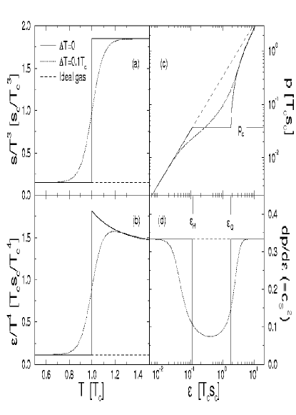
Figure 8: (a) The entropy density divided by $T^{3}$ as a function of $T$. (b) The energy density divided by $T^{4}$ as a function of $T$. (c) The pressure as a function of energy density. (d) The velocity of sound squared as a function of energy density. $c_{\rm Q}/c_{\rm H}=37/3$. Units of energy are $T_{\rm c}$, units of energy density are $T_{\rm c}s_{\rm c}$, where $s_{\rm c}\equiv(c_{\rm Q}+c_{\rm H})\,T_{\rm c}^{3}/2$. Solid line: $\Delta T=0$, dotted line: $\Delta T=0.1\,T_{\rm c}$, dashed line: ideal hadron gas.

Figs. 8 (a,b) show the entropy density divided by $T^{3}$ and the energy density divided by $T^{4}$ as functions of $T$. This representation of the equation of state is commonly used by the lattice QCD community. On the other hand, fluid dynamics requires the pressure as a function of energy density, $p(\epsilon)$, which is shown in Fig. 8 (c). The collective evolution of the fluid is, however, controlled by pressure gradients. Figure 8 (d) shows the velocity of sound squared $c_{\rm s}^{2}\equiv\D p/\D\epsilon$ (if there are no conserved charges). This quantity determines the pressure gradient $\D p$ for a given gradient in energy density $\D\epsilon$, i.e., it characterizes the capability of the fluid to perform mechanical work, or in other words, it characterizes the expansion tendency. Thus, for the equation of state with a first order phase transition, $\Delta T=0$, in the mixed phase of quark-gluon and hadronic matter, $\epsilon_{\rm H}\leq\epsilon\leq\epsilon_{\rm Q}$, the system does not perform mechanical work and therefore has no tendency to expand. As will be seen in the following this will have profound influence on the time evolution of the system.

For the equation of state with a smooth cross-over transition, $\Delta T=0.1\,T_{\rm c}$, the expansion tendency is not zero, but still greatly reduced in the transition region as compared to the ideal gas equation of state without any transition ($c_{\rm s}^{2}=1/3={\rm const.}$ for all values of $\epsilon$). The transition region $\epsilon_{\rm H}\la\epsilon\la\epsilon_{\rm Q}$ is referred to as the “soft region” of the equation of state [23]. For an equation of state with a first order transition, the point $\epsilon=\epsilon_{\rm Q}$ is called the “softest point” of the equation of state [24]. (This notion comes from considering the function $p(\epsilon)/\epsilon$ which has a minimum at $\epsilon_{\rm Q}$.)

Another quantity of interest is $\Sigma$, which determines whether matter is thermodynamically normal or anomalous. Figure 9 shows this quantity (times $Ts$) as computed from (95) for the three equations of state studied here. For $\Delta T=0$, matter becomes anomalous in the mixed phase, the other two equations of state are thermodynamically normal everywhere. (Strictly speaking, $\Sigma=0$ only vanishes in the mixed phase, but does not become negative. This is, however, sufficient for the formation of stable rarefaction shock waves.)

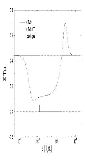
Figure 9: The quantity $\Sigma$ (times $Ts$) as a function of $\epsilon$ for $\Delta T=0$ (solid line), $\Delta T=0.1\,T_{\rm c}$ (dotted line), and the ideal hadron gas equation of state (dashed line).

Let us now consider the one-dimensional expansion of semi-infinite matter into the vacuum. Figure 10 shows temperature profiles for (a) the expansion of an ideal gas and (b,c) for the expansion with the $\Delta T=0$ equation of state. In (b) the initial energy density of semi-infinite matter is chosen to be well above $\epsilon_{\rm Q}$, the phase boundary between the quark-gluon and the mixed phase, in (c) the initial energy density is just below $\epsilon_{\rm Q}$. The dotted line in (a) indicates the initial temperature profile for all cases. The initial profile indicates a discontinuity at $x=0$ which separates two regions of constant flow, the semi-infinite slab of matter at rest to the left ($x\leq 0$), and the vacuum to the right ($x>0$). This initial condition is in fact a special case of the Riemann problem discussed in Subsection 3.3. From general arguments (see above) the solution at $t>0$ can only be a simple wave, connecting these two regions of constant flow. For the ideal hadron gas which is thermodynamically normal matter, we have seen above that this simple wave must be a continuous rarefaction wave, in this case moving to the right. As mentioned above, for such a wave the Riemann invariant ${\cal R}_{+}={\rm const.}$ everywhere, cf. (89), from which we deduce the relationship between the fluid rapidity $y$ and the energy density $\epsilon$ on the rarefaction wave:

$$y(\epsilon)=-\frac{c_{\rm s}}{1+c_{\rm s}^{2}}\,\ln\frac{\epsilon}{\epsilon_{0}}\enspace,$$ (110)

where we have used the fact that for the ideal hadron gas equation of state $p=c_{\rm s}^{2}\epsilon$ and that the initial fluid rapidity of the semi-infinite slab is zero, $y_{0}=0$. The fluid velocity on the rarefaction wave is then given by $v(\epsilon)=\tanh y(\epsilon)$. Finally, the position at which one finds a given energy density $\epsilon$ at time $t$ can be deduced by integrating (90) for the non-trivial ${\cal C}_{-}$ characteristics:

$$x(\epsilon)=\frac{v(\epsilon)-c_{\rm s}}{1-v(\epsilon)\,c_{\rm s}}\,t\enspace,$$ (111)

where we have used the fact that the initial position of the simple wave is at $x=0$ and that $c_{\rm s}={\rm const.}$ for the ideal hadron gas equation of state (we have assumed that the hadron gas consists of massless, i.e., ultrarelativistic pions, for which $c_{\rm s}^{2}=1/3$). Equation (111) tells us that the rarefaction wave moves with sound velocity into the semi-infinite slab of matter (to the left), $x_{\rm A}=-c_{\rm s}t$, and with the velocity of light into the vacuum (to the right), $x_{\rm B}=t$.

Figure 10: Temperature profiles for the expansion of semi-infinite matter into vacuum. (a) Ideal hadron gas equation of state, the dotted line indicates the initial state, the temperature is normalized to the initial temperature $T_{0}$. (b,c) Equation of state with $\Delta T=0$, in (b) the initial energy density is well above $\epsilon_{Q}$, in (c) it is just below $\epsilon_{Q}$. The temperature in (b,c) is normalized to the critical temperature $T_{\rm c}$.

The expansion in the case of a first order phase transition, $\Delta T=0$, proceeds similarly, with the exception that in the region of energy densities corresponding to the mixed phase, matter is thermodynamically anomalous, cf. Fig. 9, such that from Table 1 we conclude that the stable wave pattern is not a continuous rarefaction wave, but a rarefaction shock wave. Thus, as long as matter is in the (thermodynamically normal) quark-gluon phase, the expansion will proceed as a continuous rarefaction wave as in Fig. 10 (a), but upon entering the mixed phase (energy density $\epsilon_{\rm Q}$, temperature $T_{\rm c}$) a rarefaction shock wave will form. The state of matter emerging from this shock wave is determined from the shock equations as described in the previous subsection, i.e., it corresponds to the Chapman–Jouguet point on the Taub adiabat with center located at the phase boundary between quark-gluon and mixed phase (for more details, see [17]). Then, also the velocity of the shock $v_{\rm sh}$ in the calculational frame is determined. In general $v_{\rm sh}$ and the velocity of matter at the base of the continuous rarefaction wave are not equal. This leads to the formation of a plateau of constant flow between $x_{\rm B}$ and $x_{\rm C}$. The state of matter at the Chapman–Jouguet point corresponds to thermodynamically normal hadronic matter, so that the further expansion has to proceed as a continuous rarefaction wave. The emerging wave pattern is shown in Fig. 10 (b).

The only difference between Fig. 10 (b) and (c) is that the initial energy density in (c) is already below $\epsilon_{\rm Q}$, i.e., in the region corresponding to mixed phase. Therefore, the expansion starts out with a rarefaction shock wave, from which matter emerges at the Chapman–Jouguet point of the respective Taub adiabat with center corresponding to the initial state of matter. (Note that this Taub adiabat differs from the one in (b), since their centers are different.) Further expansion proceeds as a continuous rarefaction wave in hadronic matter.

This completes the discussion of the expansion of semi-infinite matter into vacuum and prepares us to understand the Landau model which is subject of the next subsection.

4.4 The Landau Model

The Landau model is historically the first case where fluid dynamics was applied to describe – at that time – hadron-hadron collisions [25]. Its main focus of application nowadays is, of course, nucleus-nucleus collisions. The main ideas are summarized in Fig. 11. Imagine two nuclei colliding at ultrarelativistic velocities in their center of mass. The nuclei are Lorentz-contracted to a “pancake-like” shape. In the moment of impact, nuclear matter becomes highly excited (the detailed microscopic processes which happen during this stage are of no concern for the following). In the limit that the velocities of the nuclei $v\rightarrow 1$, there will be no baryon stopping (due to the limited stopping power of nuclear matter), i.e., the baryon charges will pass through each other unscathed, leaving highly excited, net baryon-free matter in their wake. Due to Lorentz contraction, the initial extension $2\,L$ in $z$ direction of this slab of highly excited matter is much smaller than the transverse size of the slab, such that the expansion will proceed mainly in the longitudinal direction and is thus essentially one-dimensional. The Landau model assumes that the slab has no initial collective velocity and that rapid thermalization takes place which is completed at $t=0$. It is also assumed that the equation of state has the simple ultrarelativistic form $p=c_{\rm s}^{2}\epsilon$, $c_{\rm s}^{2}={\rm const.}$, i.e., that matter is thermodynamically normal for all $\epsilon$. (The original idea of Landau actually was that the baryons are immediately stopped in the collision through compressional shock waves. Data from heavy-ion experiments at BNL-AGS and CERN-SPS prove that this picture is unrealistic, due to the aforementioned finite stopping power of nuclear matter. However, since the collision is ultrarelativistic, the thermal energy in the highly excited slab is much larger than the chemical energy associated with the conservation of baryon charge. Therefore, to good approximation, $\mu_{\rm B}=n_{\rm B}=0$, and the further evolution of the slab will be identical to what is discussed here.)

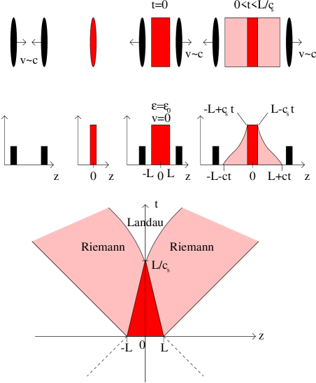
Figure 11: The Landau model for nuclear collisions. See text for details.

For $t>0$, the slab starts to expand. As in the expansion of semi-infinite matter discussed in the previous subsection, rarefaction waves will form. For thermodynamically normal matter, these are continuous (Riemann) rarefaction waves which travel into the slab with sound velocity. Therefore, they will meet at the center of the slab (here chosen to be the origin $z=0$) at a time $L/c_{\rm s}$. For times $t>L/c_{\rm s}$, these waves overlap and the solution becomes more complicated. In a region near the light cone, the solution will remain a Riemann rarefaction wave, therefore we term this region the Riemann region. In the center where the Riemann rarefaction waves overlap, however, the solution is no longer a simple wave (indeed, only two regions of constant flow have to be connected by a simple wave [18], for two simple waves no such theorem exists). For $c_{\rm s}^{2}={\rm const.}$ the solution can still be given in closed analytic form [25], although the derivation is rather complicated. However, since two of our equations of state do not have constant velocities of sound, we have to resort to numerical solution methods, such as the relativistic HLLE discussed above. In principle, numerical algorithms can deal with arbitrary (physically reasonable) equations of state, and are therefore well able to handle this problem (although one should test them thoroughly for test cases where analytical solutions are known [17, 20]).

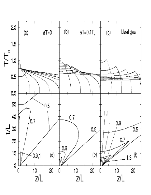
Figure 12: Expansion in the Landau model for $\Delta T=0$ (a,d), $\Delta T=0.1\,T_{\rm c}$ (b,e), and the ideal gas equation of state (c,f). (a–c) show temperature profiles for different times, (d–f) show the corresponding isotherms in the $t-z$ plane (numbers are temperatures in units of $T_{\rm c}$). The initial energy density is $\epsilon_{0}=1.875\,T_{\rm c}s_{\rm c}$ in all cases.

In Fig. 12 numerical solutions for the Landau model are presented for the three different equations of state of Fig. 8. The initial energy density is $\epsilon_{0}=1.875\,T_{\rm c}s_{\rm c}$ which is slightly larger than $\epsilon_{\rm Q}$. In Figs. 12 (a–c) temperature profiles are shown for different times $t$ and for the $z>0$ half plane (the solution in the other half plane is the respective mirror image). For $\Delta T=0$, Fig. 12 (a), one clearly observes the rarefaction shock wave which, for this initial energy density is almost stationary. Hadronic matter is expelled from the shock until the energy in the interior of the slab decreases below $\epsilon_{\rm H}$ and the shock vanishes. For $\Delta T=0.1\,T_{\rm c}$, Fig. 12 (b), no shock is formed, although the variation of the velocity of sound in the mixed phase, Fig. 8 (d), leads to shapes for the continuous rarefaction waves which differ strongly from those for a constant velocity of sound, Fig. 12 (c). Note the kink in the temperature profiles in the latter case which indicate the position where the Landau solution matches to the Riemann rarefaction wave. Note also the difference in the initial temperatures for the three cases although the initial energy density is the same. This is a consequence of the different number of degrees of freedom for the three equations of state at high energy densities.

In Figs. 12 (d–f) corresponding isotherms are shown in the $t-z$ plane. The most pronounced feature is that due to the small propagation velocity of the rarefaction wave, the system stays hot for a much longer time span for the $\Delta T=0$ equation of state, Fig. 12 (d), than for the ideal gas, Fig. 12 (f). This is in agreement with the general argument presented earlier that the softening of the equation of state in the mixed phase region leads to a reduced expansion tendency and thus to a “stalled” expansion of the system. The softening of the equation of state is also the reason why the expansion for the $\Delta T=0.1\,T_{\rm c}$ equation of state, Fig. 12 (e), is delayed in comparison to the ideal gas case, although no rarefaction waves are formed. For a quantitative analysis of the delayed expansion in the Landau model see [23].

4.5 The Bjorken Model

One of the main assumptions of Landau’s model is that the initial collective velocity of the slab of excited matter vanishes. However, this cannot be quite true on account of the following argument. In the limit $v\rightarrow 1$, the size of the nuclei in longitudinal direction goes to zero, and there is no scale in the problem at all. In this case, the collective velocity of matter in the slab has to be of the scaling form $v=z/t$. The consequences of this special form for the longitudinal fluid velocity were first investigated in [26, 27], again with respect to possible applications in hadron-hadron collisions. Bjorken [28] was the first to discuss it in the framework of nuclear collisions.

The main ideas of the so-called Bjorken model are summarized in Fig. 13. As in the Landau model, two ultrarelativistic, Lorentz-contracted nuclei collide at $z=0$ and $t=0$ (the moment of complete overlap) in the center of mass frame of the collision. Due to the limited amount of nuclear stopping power, the baryon charges keep on moving along the light cone, while microscopic collision processes (the nature of which is of no concern for the following) lead to the formation of a region of highly excited, net charge free matter in the wake of the nuclei. In contrast to the Landau model, however, the collective velocity in this region is of the scaling form $v=z/t$. The region of highly excited matter is supposed to rapidly equilibrate locally within a time span $\tau_{0}$ (which is of the order of a fm or less), and the further evolution of the system can be described in terms of ideal fluid dynamics. One important point is that, due to the absence of a scale, physics has to be the same for matter at different longitudinal coordinate $z$ if compared at the same proper time $\tau=t\sqrt{1-v^{2}}=\sqrt{t^{2}-z^{2}}$. (Such curves of constant $\tau$ describe hyperbola in space-time.) Thus, the initial thermodynamic state of all fluid elements is the same at the same proper time $\tau_{0}$.

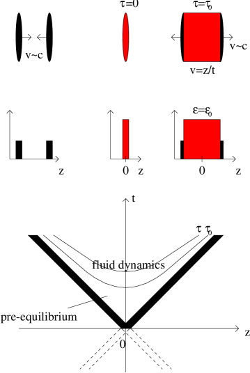
Figure 13: The Bjorken model for nuclear collisions. See text for details.

If the longitudinal velocity profile is enforced by the scaling argument, the fluid-dynamical solution simplifies in fact considerably. To see this, change the variables $t,\,z$ in the conservation laws for one-dimensional longitudinal motion in the absence of conserved charges,

$$\partial_{t}\,T^{00}+\partial_{z}\,T^{z0}=0\,\,\,,\,\,\,\,\partial_{t}\,T^{0z}+\partial_{z}\,T^{zz}=0\enspace,$$ (112)

to the variables $\tau=\sqrt{t^{2}-z^{2}}$, which is the proper time of a fluid element, and $\eta={\rm Artanh}\,v={\rm Artanh}[z/t]$, which is the rapidity of a fluid element. Then, the coupled system of partial differential equations (112) decouples:

$$\left.\frac{\partial\epsilon}{\partial\tau}\right|_{\eta}+\frac{\epsilon+p}{\tau} = 0\enspace,$$ (113)

$$\left.\frac{\partial p}{\partial\eta}\right|_{\tau} = 0\enspace.$$ (114)

The second equation (114) has the interesting consequence that there is no pressure gradient between adjacent fluid elements (the one at $\eta$ and the one at $\eta+\D\eta$). At first glance this would seem to indicate that there is no expansion of the fluid at all. This, however, is not true, since the fluid velocity is certainly finite, $v=z/t$. The answer is that the new coordinates $(\tau,\eta)$ already take the scaling expansion into account: a fluid element at $\eta$ with a width $\Delta\eta$ in fact “grows” in longitudinal direction by an amount $\D z=\D t\,\Delta\eta$ during the time span $\D t$ .

Another consequence of (114) is derived from the Gibbs–Duhem relation:

$$\left.\frac{\partial p}{\partial\eta}\right|_{\tau}=s\left.\frac{\partial T}{\partial\eta}\right|_{\tau}+\sum_{i=1}^{n}n_{i}\left.\frac{\partial\mu_{i}}{\partial\eta}\right|_{\tau}=0\enspace.$$ (115)

This equation means that for vanishing conserved charges $n_{i}=0$, $i=1,\ldots,n$, the temperature has to be constant along curves of constant $\tau$, i.e., along the space-time hyperbola shown in Fig. 13 ($\eta$ varies along these curves). In the general case of non-zero net charges, however, only the particular combination of charge densities, entropy density, and derivatives of $T$ and the $\mu_{i}$ appearing in (115) has to vanish along curves of constant $\tau$. Equation (114) represents the principle of “boost invariance” commonly associated with the Bjorken model: at constant $\tau$ the pressure is independent of the longitudinal rapidity, i.e., it is the same in fluid elements with different $\eta$, or in other words, it does not change if one performs a longitudinal boost to a different reference frame. This is a consequence of the scaling form for the longitudinal velocity.

Equation (113) also has an interesting consequence. With the first law of thermodynamics, one derives as usual the conservation of the entropy current which now takes the form

$$\left.\frac{\partial s}{\partial\tau}\right|_{\eta}+\frac{s}{\tau}=0\enspace,$$ (116)

which can be immediately integrated to give

$$s\,\tau=s_{0}\tau_{0}={\rm const.}$$ (117)

at constant $\eta$. The constant may in principle differ for different $\eta$, but since the initial thermodynamic state along $\tau_{0}$ was the same for all $\eta$, that constant will also be the same for all $\eta$ at other $\tau>\tau_{0}$. Equation (117) is interesting because it tells us that the entropy density decreases inversely proportional to $\tau$ independent of the equation of state of the fluid. The time evolution for energy density, pressure, or temperature might depend on the equation of state, but not the one for the entropy density.

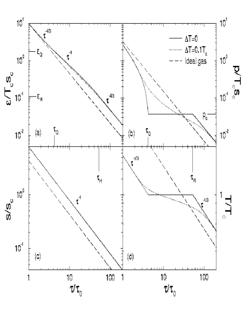
Figure 14: Proper time evolution for (a) energy density, (b) entropy density, (c) pressure, and (d) temperature in the Bjorken model for nuclear collisions (longitudinal expansion only). Solid line: $\Delta T=0$, dotted line: $\Delta T=0.1\,T_{\rm c}$, dashed line: ideal gas equation of state. The initial energy density is $\epsilon_{0}=10\,T_{\rm c}s_{\rm c}$.

This is confirmed in Fig. 14, where the evolution of (a) the energy density, (b) the entropy density, (c) the pressure, and (d) the temperature is shown as a function of proper time $\tau$ for the three equations of state ($\Delta T=0$, $\Delta T=0.1\,T_{\rm c}$, and the ideal hadron gas). Note that in the quark-gluon as well as the hadron phase, where $p\sim c_{\rm s}^{2}\,\epsilon$ with $c_{\rm s}^{2}=1/3$, Eq. (113) yields

$$\epsilon\sim\tau^{-4/3}\enspace,$$ (118)

For the $\Delta T=0$ equation of state, $p=p_{\rm c}={\rm const.}$ in the mixed phase, and (113) yields the cooling law

$$\epsilon\sim\tau^{-1}\enspace.$$ (119)

This is interpreted as follows. The longitudinal scaling expansion dilutes the system $\sim\tau^{-1}$. If no mechanical work is performed, like in the mixed phase where $\D p\equiv 0$, only this geometrical dilution determines the (proper) time evolution of the energy density. In the phase where $\D p=c_{\rm s}^{2}\,\D\epsilon$, however, additional mechanical work is performed, and the system cools faster, $\epsilon\sim\tau^{-(1+c_{\rm s}^{2})}=\tau^{-4/3}$. The faster cooling is confirmed studying the temperature evolution, Fig. 14 (d). For $p=c_{\rm s}^{2}\,\epsilon$, $c_{\rm s}^{2}={\rm const.}$, and vanishing net charges, one deduces from $\D p=c_{\rm s}^{2}\,\D\epsilon=s\,\D T=(\epsilon+p)\,\D T/T=(1+c_{\rm s}^{2})\,\epsilon\,\D T/T$, that $\epsilon\sim T^{1+c_{\rm s}^{-2}}$ and consequently, in the hadron and quark-gluon phase

$$T\sim\tau^{-1/3}\enspace,$$ (120)

while in the mixed phase one deduces from $\D p=s\,\D T\equiv 0$ that

$$T={\rm const.}\enspace.$$ (121)

This expectation is confirmed in Fig. 14 (d).

Of course, in reality the expansion of the system will not only be purely longitudinal. The “Bjorken cylinder” will also expand transversally. The principle of boost invariance allows us to focus on the transverse expansion at $z=\eta=0$ only, and reconstruct the fluid properties at a different $\eta$ by performing a longitudinal boost with boost rapidity $\eta$. For the sake of simplicity, let us assume that the system is cylindrically symmetric in the transverse direction and that the initial energy density profile is of the form

$$\epsilon(\vec{r},\tau_{0},\eta=0)=\epsilon_{0}\,\Theta(R-|\vec{r}|)\enspace,$$ (122)

where $R$ is the transverse radius of the Bjorken cylinder. In cylindrical coordinates and at $z=\eta=0$, the conservation equations read ($T^{00}\equiv E,\,T^{0r}\equiv M,\,v_{r}\equiv v$):

$$\partial_{t}\,E+\partial_{r}\,\left[(E+p)v\right] = -\left(\frac{v}{r}+\frac{1}{t}\right)(E+p)\enspace,$$ (123)

$$\partial_{t}\,M+\partial_{r}\,(Mv+p) = -\left(\frac{v}{r}+\frac{1}{t}\right)M\enspace.$$ (124)

Although these equations have no longer a simple analytical solution, the assumption of cylindrical symmetry has reduced the originally three-dimensional problem to an effectively one-dimensional problem. Indeed, for vanishing right-hand sides the solution of (123), (124) with the initial condition (122) is identical to the one of the Landau model with the substitutions $z\rightarrow r$ and $L\rightarrow R$. The right-hand sides just lead to an additional reduction of $E$ and $M$ from the cylindrical geometry, $v/r$, and from longitudinal scaling, $1/t$.

This observation, combined with the method of operator splitting discussed previously, suggests the following simple solution scheme (also known as Sod’s method [16, 29]): equations (123), (124) are of the type

$$\partial_{t}\,U+\partial_{x}\,F(U)=-G(U)\enspace.$$ (125)

The operator splitting method allows to construct the solution by first solving the one-dimensional partial differential equation

$$\partial_{t}\,U+\partial_{x}\,F(U)=0\enspace,$$ (126)

(for instance with the relativistic HLLE scheme discussed above), which yields a prediction $\tilde{U}$ for the true solution $U$. In a second step one corrects this prediction by solving the ordinary differential equation

$$\frac{\D U}{\D t}=-G(U)\enspace,$$ (127)

which is numerically realized as [30]

$$U=\tilde{U}-\Delta t\,G(\tilde{U})\enspace.$$ (128)

The transverse expansion of the Bjorken cylinder at $z=0$ is shown in Fig. 15 for $\tau_{0}=0.1\,R$ and $\epsilon_{0}=18.75\,T_{\rm c}s_{\rm c}$. One immediately recognizes the qualitative similarities with the Landau expansion, like the delay in the expansion for the two equations of state with a (phase) transition as compared to the expansion with an ideal hadron gas equation of state. The additional geometrical dilution, however, leads in general to a faster cooling overall and quantitatively different shapes for the temperature profiles and the isotherms in the $t-r$ plane.

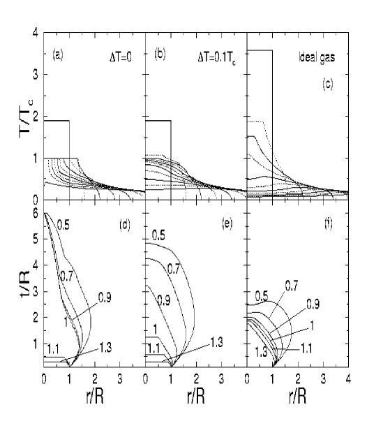
Figure 15: Transverse expansion of the Bjorken cylinder for $\Delta T=0$ (a,d), $\Delta T=0.1\,T_{\rm c}$ (b,e), and the ideal gas equation of state (c,f). (a–c) show temperature profiles for different times, (d–f) show the corresponding isotherms in the $t-r$ plane (numbers are temperatures in units of $T_{\rm c}$). The initial energy density is $\epsilon_{0}=18.75\,T_{\rm c}s_{\rm c}$ in all cases.

Let us further quantify the time delay in the expansion induced by the transition in the equation of state. In general, the system will decouple into free-streaming particles once the temperature drops below a certain “freeze-out” temperature $T_{\rm fo}$, see Section 5 below. From comparison with experimental data, this freeze-out temperature is estimated to be on the order of 100 MeV. Let us therefore define a “lifetime” of the system as the time when the $T=0.7\,T_{c}$ isotherm crosses the origin at $r=0$ in Figs. 15 (d–f). This lifetime is shown in Figs. 16 (a,b) as function of the initial energy density $\epsilon_{0}$ of the cylinder. One observes a maximum of the such defined lifetime at initial energy densities around $40\,T_{\rm c}s_{\rm c}\sim 30\,{\rm GeVfm}^{-3}$. At these initial energy densities, the prolongation of the lifetime over the respective ideal hadron gas value is about a factor of 2 (for $\Delta T=0.1\,T_{\rm c}$) to 3 (for $\Delta T=0$).

The prolongation of the lifetime is due to the softening of the equation of state in the phase transition region. It is, however, interesting that the maximum in the lifetime does not occur around initial energy densities corresponding to $\epsilon_{\rm Q}$ (as is the case in the Landau model [23]), but at much larger initial energy densities. The reason for this is the strong longitudinal dilution of the system on account of the scaling profile $v_{z}=z/t$. In order to see a large effect of the softening of the equation of state in the phase transition region on the expansion dynamics, the transverse (Landau-like) expansion has to be the dominant cooling mechanism for the system. The Bjorken scaling expansion does not account for the reduced expansion tendency of the system in the transition region, it enforces an expansion velocity $v_{z}=z/t$ irrespective of the equation of state. In order to have the transverse expansion dominate the cooling of the system, one has to start the expansion at higher initial energy densities such that the system spends enough time in the mixed phase for the (slow) rarefaction shock to reach the origin. The initial energy density in Fig. 15 was intentionally selected to maximize this effect.

Initial energy densities on the order of $10-30\,{\rm GeVfm}^{-3}$ are expected to be reached at the RHIC collider. In order to experimentally observe the prolongation of the lifetime as seen in Figs. 16, one has to find a corresponding experimental observable. An obvious candidate is the ratio of the “out” to the “side” radius of two-particle correlation functions. The “out” radius is proportional to the duration of particle emission from a source, while the “side” radius is proportional to the transverse dimension of the source (cf. [31] for a very detailed, pedagogical discussion). Since the transverse radius of the source is approximately the same in all cases, cf. Fig. 15 (a–c), the ratio $R_{\rm out}/R_{\rm side}$ seems to be a good generic measure for the lifetime. Moreover, in forming the ratio the dependence on the overall (unknown) spatial size of the source as well as effects from the collective expansion are expected to cancel. The ratio $R_{\rm out}/R_{\rm side}$ is plotted in Figs. 16 (c,d) for pions with mean transverse momenta $K_{\perp}=300$ MeV. (Details on how to compute this quantity can be found in [30, 32].) As one observes, $R_{\rm out}/R_{\rm side}$ nicely reflects the excitation function of the lifetime of the system.

Figure 16: Lifetime of the system as a function of $\epsilon_{0}$ for the Bjorken cylinder expansion, $\tau_{0}=0.1\,T_{\rm c}$. (a) $\Delta T=0$ (solid) vs. ideal hadron gas (dashed), (b) $\Delta T=0.1\,T_{\rm c}$ (dotted) vs. ideal hadron gas (dashed). (c,d) the corresponding ratio $R_{\rm out}/R_{\rm side}$.

5 Freeze-Out

In this section I discuss an up to date unsolved problem in the application of relativistic fluid dynamics to describe nuclear collisions, namely the so-called “freeze-out” process. Given an initial condition, fluid dynamics describes the evolution of the system in the whole forward lightcone, Fig. 17 (a). However, as we have seen above, at all times near the boundary to the vacuum, as well as everywhere in the late stage of the evolution, the energy density becomes arbitrarily small, i.e., the system is rather cold and dilute. In this space-time region the assumption of local thermodynamical equilibrium is no longer justified, because the particle scattering cross section $\sigma$ is finite, such that for small particle densities $n$ the particle scattering rate, $\Gamma\sim\sigma n$, becomes on the order of the inverse system size, $\Gamma\sim R^{-1}$. At this point, the scattering rate is too small to maintain local thermodynamical equilibrium and the particles decouple from the fluid evolution. In this space-time region, a kinetic description for the particle motion would be more appropriate. One should therefore not solve fluid-dynamical equations in the whole forward lightcone, but only inside a space-time region of sufficiently large energy and particle densities, while outside this region, the particle motion should be described by kinetic theory, Fig. 17 (b).

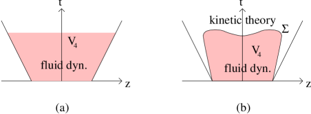
Figure 17: (a) Conventional fluid-dynamical description in the whole forward lightcone. (b) Fluid dynamics describes the evolution of the system inside $V_{4}$, while kinetic theory describes the motion of the frozen-out particles outside $V_{4}$.

The boundary $\Sigma$ between the two regions is determined by a criterion which compares local scattering rates with the system size, as discussed above. The obvious difficulty with this more realistic description of the system’s evolution is that this boundary has to be determined dynamically, i.e., not only has one to allow for particles decoupling from the fluid, but also for the reverse process of particles entering the fluid from the kinetic region. (This can happen since the particles still, albeit rarely, collide in the kinetic region.) A consistent treatment of this problem is rather complicated, since one has to solve kinetic in addition to the fluid-dynamical equations. No serious attempt has been made so far.

Instead, the following approximate solution has been extensively employed:

1. One assumes that fluid dynamics gives a reasonable description for the evolution of the system in the whole forward lightcone.

2. One determines the “decoupling” surface $\Sigma$ a posteriori, once the evolution of the fluid is known.

3. The “thickness” of $\Sigma$ is assumed to be infinitesimal.

4. One assumes that particles crossing $\Sigma$ have completely decoupled from the system, they stream freely towards the detectors without any further collisional interaction (“freeze-out”). This means that they do not change their momentum and energy once they have crossed $\Sigma$.

A very popular argument in order to determine $\Sigma$ is the following. Since $n\sim T^{3}$, the scattering rate $\Gamma\sim T^{3}$ (for constant cross section $\sigma$), i.e., if the temperature falls below a certain so-called “freeze-out” temperature $T_{\rm fo}$, the criterion $\Gamma\la R$ is fulfilled, and particles decouple from the system. In this case, $\Sigma$ is just given by the isotherm $T=T_{\rm fo}$ (use of this argument was already made above in the discussion of the “lifetime” of the system).

Note that assumption 3. is a strong idealization and actually rather questionable, because in reality $\Sigma$ is a space-time region of finite thickness, inside which non-equilibrium, dissipative effects become gradually more and more important (the more dilute the fluid becomes), until ultimately all interactions between particles cease and, when leaving $\Sigma$, they stream freely towards the detectors.

Nevertheless, with the above assumptions, one can readily compute the single inclusive spectra of particles reaching the detector. Immediately before the particles decouple from the fluid evolution, i.e., before they cross $\Sigma$, they are still in local thermodynamical equilibrium such that their phase space distribution is given by $f_{0}(k,x)$, Eq. (20). It is reasonable to assume that this phase space distribution is not changed much when they move a small distance along their worldlines, which carries them across $\Sigma$ into the region of free-streaming. In that region, however, there are no collisions which could further change $f_{0}$. Therefore, the phase space distribution of “frozen-out” particles is (approximately) the same as in local equilibrium. The total number of particles crossing a small surface element $\D\Sigma$ of $\Sigma$ is then given by

$$N_{\Sigma}\equiv\D\Sigma_{\mu}N^{\mu}=\int\frac{\D^{3}\vec{k}}{E}\,\D\Sigma\cdot k\,f_{0}(k,x)\enspace,$$ (129)

$N^{\mu}$ being the (kinetic) particle number 4-current. The invariant momentum spectrum of particles crossing that surface element is consequently

$$E\,\frac{\D N_{\Sigma}}{\D^{3}\vec{k}}=\D\Sigma\cdot k\,f_{0}(k,x)\enspace.$$ (130)

Finally, the invariant momentum spectrum (the single inclusive spectrum) of particles crossing the complete “freeze-out” surface $\Sigma$ is

$$E\frac{\D N}{\D^{3}\vec{k}}=\int_{\Sigma}\,E\,\frac{\D N_{\Sigma}}{\D^{3}\vec{k}}=\int_{\Sigma}\D\Sigma\cdot k\,f_{0}(k,x)\enspace.$$ (131)

This equation is known as the Cooper–Frye formula [26], and is used in almost all fluid-dynamical applications to heavy-ion collisions to compute the single inclusive spectra of particles.

There is, however, a problem with this formula [33]. For time-like surfaces, i.e., where the normal vector $\D\Sigma_{\mu}$ is space-like, $\D\Sigma\cdot k$ may either be positive or negative, depending on the value and direction of $k^{\mu}$. In other words, the number of particles “freezing out” from a certain time-like surface element $\D\Sigma$ can become negative. This is clearly unphysical, since the number of particles decoupling from the system must be positive definite. For space-like surfaces (with a time-like normal vector) as well as for time-like surface elements where $\D\Sigma\cdot k>0$, the Cooper-Frye formula gives a physically reasonable, positive definite result for the number of frozen-out particles. This is illustrated in Fig. 18 which shows the rapidity distribution of particles (i.e., the invariant momentum spectrum integrated over all transverse momenta) for massless particles decoupling from a freeze-out isotherm $T_{\rm fo}=0.4\,T_{0}$ in the Landau model with a $p=\epsilon/3$ equation of state. One clearly notices the negative particle numbers at midrapidity coming from the time-like parts of the isotherm.

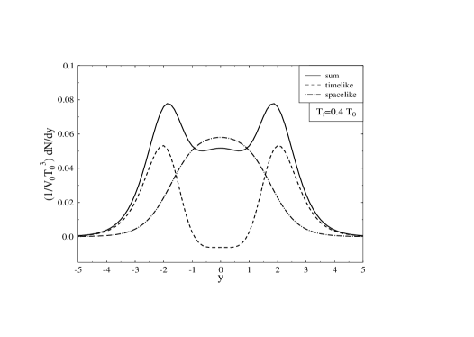
Figure 18: The rapidity distribution for freeze-out along the $T_{\rm fo}=0.4\,T_{0}$ isotherm in the Landau model. Solid: full distribution, dotted: particles from time-like parts of the isotherm, dash-dotted: particles from space-like parts of the isotherm.

This contradiction is readily resolved noting that the Cooper-Frye formula does not really determine the number of particles decoupling from the system, but merely the number of particle worldlines crossing a surface element $\D\Sigma$ (and then integrated over the whole surface $\Sigma$). For time-like surface elements, there is of course the possibility that for certain $k^{\mu}$ the respective worldlines cross $\D\Sigma$ in the “wrong” direction, i.e., the momenta of the particles point back into the region of fluid, cf. Fig. 19. In particular, for the $T_{\rm fo}=0.4\,T_{0}$ isotherm, which moves away from the $t$-axis in the $t-z$ plane, those are particles with vanishing momentum component in $z$ direction, because their worldlines are parallel to the $t$-axis. Particles with $p^{z}=0$, however, also have vanishing longitudinal rapidity $y=0$, and that is the reason why these negative particle numbers appear at midrapidity in Fig. 18. While this explains the negative contributions in the Cooper-Frye formula, it also invalidates this formula as the correct prescription to calculate the spectra of frozen-out particles, if parts of the decoupling surface are time-like.

Figure 19: Explanation for the negative number of frozen-out particles in the Cooper-Frye formula.

One suggestion to circumvent this problem was to compute the final spectra only from contribution of particles which cross the space-like parts of $\Sigma$. Of course, as can be seen by comparing the dash-dotted with the solid line in Fig. 18, the final spectra are dramatically different. Moreover, by neglecting particles crossing the time-like parts, the absolute number of frozen-out particles will also differ in the two cases. Note that the $\D N/\D y$ distribution for particles from the space-like parts of the decoupling isotherm has a Gaussian shape in the Landau model. This was already pointed out in Landau’s original paper [25] and has since survived as the generic (but wrong) statement that Landau’s model gives rise to Gaussian rapidity distributions. In fact, there is no decoupling temperature where the full rapidity distribution including particles from the time-like parts resembles a Gaussian, cf. Fig. 20.

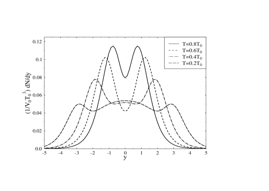
Figure 20: Rapidity distributions for freeze-out along isotherms with $T_{\rm fo}=0.8\,T_{0}$ (solid), $0.6\,T_{0}$ (dashed), $0.4\,T_{0}$ (dash-dotted), and $0.2\,T_{0}$ (long dashed) in the Landau model with a $p=\epsilon/3$ equation of state.

Another suggestion to circumvent the problem of negative particle numbers is, instead of freezing out along an isotherm which has time-like parts, to freeze out along a surface which is space-like everywhere, for instance, a curve of constant time in the center-of-mass frame, cf. Fig. 21. In this case, all particles are accounted for, since the decoupling surface is bounded by the lightcone, and no particle can escape through the lightcone. The problem is, that also in this case, the spectra differ considerably from a freeze-out at constant temperature, cf. Fig. 22. This uncertainty is clearly unwanted when one wants to quantitatively compare fluid-dynamical model predictions with experimental data.

Figure 21: A curve of constant time in the center-of-mass frame as freeze-out isotherm.

Figure 22: The rapidity distribution for freeze-out along curves of constant time in the center-of-mass frame defined by requiring the average temperature to be $\langle T\rangle=0.8\,T_{0}$ (solid), $0.6\,T_{0}$ (dashed), $0.4\,T_{0}$ (dash-dotted), and $0.2\,T_{0}$ (long dashed) in the Landau model with a $p=\epsilon/3$ equation of state.

The correct formula to compute the number of particles which physically decouple from the system was given in [33]:

$$E\frac{\D N}{\D^{3}\vec{k}}=\int_{\Sigma}\D\Sigma\cdot k\,f_{0}(k,x)\,\Theta(\D\Sigma\cdot k)\enspace.$$ (132)

The additional $\Theta$-function ensures that negative contributions to the Cooper–Frye formula are cut off. The problem with this formula is that these negative contributions were necessary to globally conserve energy, momentum and net charge number, cf. the derivation of the conservation equations in Section 2. The violation of the conservation equations introduced by the freeze-out prescription (132) can, however, be circumvented by adjusting temperature, chemical potential, and the average particle 4-velocity in the single-particle distribution function $f_{0}(k,x)$ in (132) in such a way as to preserve the conservation laws. In other words, one must not use temperature, chemical potential, and fluid 4-velocity on the fluid side of the freeze-out surface in (132), but modified values which ensure that energy, momentum, and net charge is conserved. One way to achieve this is to assume that the freeze-out surface actually is a conventional fluid-dynamical discontinuity across which energy, momentum, and net charge number are conserved. Solving the corresponding algebraic conservation equations (with energy-momentum tensor and net charge current on the post freeze-out side of the discontinuity constructed from (21,22) with $f_{0}(k,x)$ replaced by $f_{0}(k,x)\,\Theta(\D\Sigma\cdot k)$) yields the required modified values for temperature, chemical potential, and average particle 4-velocity on the post freeze-out side. For more details, see [33, 34]. However, it still remains to be shown with an explicit calculation whether this suggestion to solve the freeze-out problem is viable in the general case.

References

- 1. H. Stöcker and W. Greiner, Phys. Rep. 137, 277 (1986)
- 2. R.B. Clare and D.D. Strottman, Phys. Rep. 141, 177 (1986)
- 3. L.P. Csernai, Introduction to relativistic heavy ion collisions (Wiley, New York, 1994)
- 4. see, for instance: E. Laermann, Nucl. Phys. A 610, 1 (1996)
- 5. L.D. Landau and E.M. Lifshitz, Fluid mechanics (Pergamon, New York, 1959)
- 6. S.R. deGroot, W.A. van Leeuwen, and Ch.G. van Weert, Relativistic Kinetic Theory (North-Holland, Amsterdam, 1980)
- 7. W.A. Hiscock and L. Lindblom, Ann. Phys. 151, 466 (1983); Phys. Rev. D 31, 725 (1985); Phys. Rev. D 35, 3723 (1987)
- 8. I. Müller, Z. Phys. 198, 329 (1967)
- 9. W. Israel, Ann. Phys. 100, 310 (1976); J.M. Stewart, Proc. Roy. Soc. A 357, 59 (1977); W. Israel and J.M. Stewart, Ann. Phys. 118, 341 (1979)
- 10. L. Mornas and U. Ornik, Nucl. Phys. A 587, 828 (1995)
- 11. M. Prakash, M. Prakash, R. Venugopalan, and G. Welke, Phys. Rep. 227, 321 (1993)
- 12. A.A. Amsden, A.S. Goldhaber, F.H. Harlow, and J.R. Nix, Phys. Rev. C 17, 2080 (1978); I.N. Mishustin, V.N. Russkikh, and L.M. Satarov, Nucl. Phys. A 494, 595 (1989); J. Brachmann, A. Dumitru, J.A. Maruhn, H. Stöcker, W. Greiner, and D.H. Rischke, Nucl. Phys. A 619, 391 (1997)
- 13. To my knowledge, this treatment of the transformation problem is due to B. Kämpfer.
- 14. V. Schneider et al., J. Comput. Phys. 105, 92 (1993)
- 15. A. Harten, P.D. Lax, and B. van Leer, SIAM Rev. 25, 35 (1983); B. Einfeldt, SIAM J. Numer. Anal. 25, 294 (1988)
- 16. M. Holt, Numerical methods in fluid dynamics, Springer Series in Comput. Physics (Springer, Berlin, 1977)
- 17. D.H. Rischke, S. Bernard, and J.A. Maruhn, Nucl. Phys. A 595, 346 (1995)
- 18. R. Courant and K.O. Friedrichs, Supersonic Flow and Shock Waves (Springer, New York, 1985)
- 19. A.M. Taub, Phys. Rev. 74, 328 (1948)
- 20. D.H. Rischke, Y. Pürsün, and J.A. Maruhn, Nucl. Phys. A 595, 383 (1995)
- 21. P. Danielewicz and P.V. Ruuskanen, Phys. Rev. D 35, 344 (1987)
- 22. A. Chodos, R.L. Jaffe, K. Johnson, C.B. Thorn, and V.F. Weisskopf, Phys. Rev. D 9, 3471 (1974)
- 23. D.H. Rischke and M. Gyulassy, Nucl. Phys. A 597, 701 (1996)
- 24. C.M. Hung and E.V. Shuryak, Phys. Rev. Lett. 75, 4003 (1995)
- 25. L.D. Landau and S.Z. Belenkii, Uspekhi Fiz. Nauk 56, 309 (1955)
- 26. F. Cooper, G. Frye, and E. Schonberg, Phys. Rev. D 11, 192 (1975)
- 27. C. Chiu and K.H. Wang, Phys. Rev. D 12, 272 (1975)
- 28. J.D. Bjorken, Phys. Rev. D 27, 140 (1983)
- 29. G.A. Sod, J. Fluid Mech. 83, 785 (1977)
- 30. D.H. Rischke and M. Gyulassy, Nucl. Phys. A 608, 479 (1996)
- 31. U. Heinz, proceedings of the International Summer School on Correlations and Clustering Phenomena in Subatomic Physics, Dronten, Netherlands, August 5–16, 1996, e-print archive nucl-th/9609029
- 32. S. Bernard, D.H. Rischke, J.A. Maruhn, and W. Greiner, Nucl. Phys. A 625, 473 (1997)
- 33. K.A. Bugaev, Nucl. Phys. A 606, 559 (1996)
- 34. C. Anderlik, Z.I. Lazar, V.K. Magas, L.P. Csernai, H. Stöcker, and W. Greiner, e-print archive nucl-th/9808024