On isovector meson exchange currents in the Bethe-Salpeter approach

Abstract

We investigate the nonrelativistic reduction of the Bethe-Salpeter amplitude for the deuteron electrodisintegration near threshold energies. To this end, two assumptions have been used in the calculations: 1) the static approximation and 2) the one iteration approximation. Within these assumptions it is possible to recover the nonrelativistic result including a systematic extension to relativistic corrections. We find that the so-called pair current term can be constructed from the $P$-wave contribution of the deuteron Bethe-Salpeter amplitude. The form factor that enters into the calculation of the pair current is constrained by the manifestly gauge independent matrix elements.

PACS: 21.45.+v, 25.30.Fj, 24.10.Jv

I Introduction

In recent years, the discussion of relativistic issues in the reactions involving the deuteron has become more and more important. Some well known examples for a clear experimental evidence have been found in the electromagnetic disintegration [1, 2]. This results are supported by a recent analysis of polarization observables of the deuteron in a relativistic framework [3, 4]. Also, the persistent difference between theory and experiment in polarization observables of proton deuteron scattering have been argued to be of relativistic origin [5]. It is expected that the interpretation of new experimental results, e.g., from TJNAF, also calls for a relativistic treatment.

Meanwhile the number of theoretical investigations devoted to this question and to tackle the relativistic aspects of few body systems is increasing. One may basically recognize two lines: on one hand the majority of approaches uses a nonrelativistic scheme of calculation and take into account some leading order corrections, such as nonnucleonic degrees of freedom like mesonic exchange currents, $\Delta\Delta$-configurations, $NN^{\star}$-states and more. For a review see, e.g., Refs. [3, 4, 6, 7, 8, 9] which also contain an large number of references. Note, however, that the problem of consistency arises as has been recently pointed out again, e.g., by Ref. [10] in the context of electrodisintegration. The second line recognizes the importance of covariance [11, 12, 13].

We follow the Bethe-Salpeter approach which is covariant by construction and properly defined [14, 15, 16]. Based on the field theory of particles this approach is also consistent and automatically takes into account all relativistic effects in the two nucleon system. Because of the covariance of the Bethe-Salpeter equation the amplitudes (or vertex functions) may be written in any reference system, and one may chose a convenient one. However, practical applications are hampered by the difficulty of finding solutions of the Bethe-Salpeter equation, even in ladder approximation. Nevertheless, the activity on solving the Bethe-Salpeter equation has increased in recent years [17, 18], and by now parameterizations of the Bethe-Salpeter amplitudes in Euclidean space are available [19]. Also, useful results have been achieved by a reduction of the Bethe-Salpeter equation to a three dimensional one.

Here, we examine the nonrelativistic reduction of the Bethe-Salpeter approach to compare with the results achieved by nonrelativistic calculations. Since the problem has not been solved so far for the general case, we restrict ourself to a special process that is the disintegration of the deuteron.To this end we consider the threshold region only that exhibits already the main features to be discussed. Also, this region is dominated by a single transition amplitude to the ${}^{1}S_{0}$ final state (see, e.g., Ref. [20]) thus leading to some technical but not substantial simplifications. The extension to other partial amplitudes is straightforward but tedious, however beyond the scope of our present approach.

Indeed, the deuteron disintegration close to threshold energies has been a key reaction to establish subnucleonic degrees of freedom in nuclei [21] and it attracts continuous attention from theoretical and experimental sides. It has been an excellent paradigm to examine nonnucleonic degrees of freedom and relativistic effects. It is well known that the nonrelativistic impulse approximation fails to describe the double differential cross section at momentum transfer squared $-q^{2}>9$ fm^-2. The experimental data do not indicate the deep minimum present in the calculations [22]. To fill this minimum mesonic exchange currents have been introduced. The contributions of $\pi$-, $\rho$-currents, and $\Delta\Delta$- configurations allow one to get a satisfactory agreement with the data  [23]. The question of a consistent inclusion of all relativistic corrections (at least for the pion sector) has recently been addressed by Ref. [10] and supports the above statement. Nevertheless, some conceptional problems of the theory still remain open questions. Among them is the problem of gauge invariance and the question of the nucleon form factor to be chosen in the exchange currents contributions [24, 25, 26].

By now some relativistic methods identify corrections like meson exchange currents in the relativistic impulse approximation. It has been shown that in the framework of the light-cone approach the so-called extra components $f_{5}$ of the deuteron wave function, and $g_{2}$ of the ${}^{1}S_{0}$-wave function introduced in Ref. [27] give an expression in the nonrelativistic limit, that analytically equals to the contribution of the pair current [27]. In this context the one iteration assumption that will be explained below for solving the dynamical equation is substantial. Another important result in this context is the calculation of the static electromagnetic properties within the Bethe-Salpeter approach. It follows that the contribution of the $P$-states to the magnetic moment of the deuteron is numerically close to the contribution of mesonic currents and agrees in sign [28]. It has already been noticed earlier in the context of covariant reductions of the Bethe-Salpeter equation to three dimensional ones that negative energy components in the wave function are responsible for pair current type contributions, see, e.g., Ref. [29]. Here we show that the suggested reduction procedure leads to the same analytical structure as the nonrelativistic pair current correction.

The paper is organized as follows. Section II contains the general formulas for the deuteron disintegration amplitude in different representations. The static approximation is also discussed. The one iteration approximation is formulated in Section III where we give reasons for its validity in simple models. The derivation of the main correction is done in the Section IV. We present and discuss our results in Section V, summarize and conclude in Section VI.

II Nonrelativistic reduction of the electromagnetic current matrix element

Because of Lorentz covariance, transformation properties under parity and time reversal as well as current conservation, the general structure of the transition matrix element for the $1^{+}\rightarrow 0^{+}$ transition current near threshold can be written as [30]

$$\langle np(^{1}S_{0})|j_{\mu}|D{\cal M}\rangle=i\epsilon_{\mu\alpha\beta\gamma}\,\xi^{\alpha}_{\cal M}\,q^{\beta}\,K^{\gamma}\,V(s,q^{2}),$$ (1)

where $\xi_{\cal M}$ is the deuteron polarization four vector with projection ${\cal M}$, $K$ is the deuteron four momentum, $q=P-K$ is the four momentum transfer, $s=P^{2}=(K+q)^{2}\approx 4m^{2}$ is the squared total momentum of the $np$-pair, see Fig. 1. The scalar function $V(s,q^{2})$ may be splitted into isovector Dirac ($F^{V}_{1}$) and Pauli ($F^{V}_{2}$) contributions

$$V(s,q^{2})=V_{1}(s,q^{2})F^{(V)}_{1}(q^{2})+V_{2}(s,q^{2})F^{(V)}_{2}(q^{2}).$$ (2)

The final state of the $np$-pair is supposed to be in a ${}^{1}S_{0}$-state. This is supported by nonrelativistic calculations [23]. Eq. (1) is valid in the any reference system and the functions $V_{1,2}$ depend on the scalars $s$ and $q^{2}$ only. Current conservation is fulfilled because the tensor $\epsilon_{\mu\alpha\beta\gamma}$ that appears in Eq. (1) is antisymmetric.

To calculate the functions $V_{1,2}$ from the underlying dynamics in the Bethe-Salpeter approach, two representations of the Bethe-Salpeter amplitude may be used in concrete calculations: 1) the covariant representation and 2) the partial-wave representation. Using the covariant representation for the initial and final states allows us to directly read off the functions $V_{1,2}(s,q^{2})$ from the proper current matrix elements. This has been done explicitly in Ref. [30]. However, to study the relation to the nonrelativistic expressions it is more suitable to give the formulas for $V_{1,2}(s,q^{2})$ in terms of a partial-wave representation of the vertex functions. Hence, the expressions for $V_{1,2}$ can be written as

$$V_{1,2}(s,q^{2})=i\int d^{4}k\sum_{\alpha,\beta}\ G_{\alpha}(p_{0},|{\mbox{\boldmath$p$}}|)\ {\cal O}_{\alpha\beta}\ g_{\beta}(k_{0},|{\mbox{\boldmath$k$}}|),$$ (3)

where the partial vertex functions $G_{1-4}(p_{0},|{\mbox{\boldmath$p$}}|)$ represent the states ${}^{1}S_{0}^{++}$, ${}^{1}S_{0}^{--}$, ${}^{3}P_{0}^{e}$, ${}^{3}P_{0}^{o}$ of the $np$-pair, and $g_{1-8}(k_{0},|{\mbox{\boldmath$k$}}|)$ denote the states ${}^{3}S_{1}^{++}$, ${}^{3}S_{1}^{--}$, ${}^{3}D_{1}^{++}$, ${}^{3}D_{1}^{--}$, ${}^{3}P_{1}^{e}$, ${}^{3}P_{1}^{o}$, ${}^{1}P_{1}^{e}$, ${}^{1}P_{1}^{o}$ of the deuteron. We use spectroscopic notation and ($\pm$, $e/o$) as $\rho$-spin quantum numbers [31]. In general, the lengthy functions ${\cal O}_{\alpha\beta}$ depend on Lorentz scalars and the explicit expressions are omitted here. We will specify them below after having introduced appropriate approximations. The expressions for $p_{0}$ and $|{\mbox{\boldmath$p$}}|$ are given in a formally covariant way, viz.

$$p_{0}=\frac{(K+q,k+q/2)}{\sqrt{s}},\ |{\mbox{\boldmath$p$}}|=\left(\frac{(K+q,k+q/2)^{2}}{s}-(k+q/2)^{2}\right)^{1/2},$$ (4)

where $(\,,)$ denotes the Lorentz scalar product.

We note that through the use of Bethe-Salpeter vertex functions the denominators of ${\cal O}_{\cal\alpha\beta}$ appearing in Eq. (3) contain products of $(\pm M/2\pm k_{0}\pm E_{k})$ and $(\pm\sqrt{s}/2\pm p_{0}\pm E_{p})$, where $E_{p}=\sqrt{{\mbox{\boldmath$p$}}^{2}+m^{2}}$, etc. that stem from the nucleon propagators (see Fig. 1). We evaluate the integrals in the laboratory system (deuteron at rest). At threshold, because of the small deuteron binding energy, it is possible to utilize the static approximation [32] that preserves the analytical structure of Eq. (3) through the following equations

$$p_{0}=k_{0},\quad|{\mbox{\boldmath$p$}}|=|{\mbox{\boldmath$k$}}+\frac{{\mbox{\boldmath$Q$}}}{2}|=\left({\mbox{\boldmath$k$}}^{2}+\frac{{\mbox{\boldmath$Q$}}^{2}}{4}+|{\mbox{\boldmath$k$}}||{\mbox{\boldmath$Q$}}|{x}\right)^{1/2}.$$ (5)

Here and in the following we use ($\hat{\bf a}={\bf a}/|{\bf a}|$)

$$Q = |{\mbox{\boldmath$Q$}}|=((M^{2}+s-q^{2})^{2}-4M^{2}s)^{1/2}/(2M),\ {x}=\hat{\mbox{\boldmath$k$}}\cdot\hat{\mbox{\boldmath$Q$}},$$ (6)

$$q = (\omega,{\mbox{\boldmath$Q$}}),\ \omega=(s-M^{2}-q^{2})/(2M).$$ (7)

We illustrate the approximation by looking closer to the expressions involving the $(++)$ states. The full denominator of the integrand in Eq. (3) leads to a complicated pole structure and reads explicitly

$$\left(\frac{s}{4}-(k_{0}+\frac{\omega}{2})^{2}+{\mbox{\boldmath$p$}}^{2}-\sqrt{s}\left(\frac{Q^{2}}{s}(k_{0}+\frac{\omega}{2})^{2}+E_{p}^{2}\right)^{1/2}-i\epsilon\right)\left(\frac{M}{2}+k_{0}-E_{k}+i\epsilon\right).$$ (8)

Using Eq. (5), then leads to a simple pole expression for the integrand involving the denominator

$$\left(\frac{\sqrt{s}}{2}+k_{0}-E_{p}+i\epsilon\right)\left(\frac{\sqrt{s}}{2}-k_{0}-E_{p}+i\epsilon\right)\left(\frac{M}{2}+k_{0}-E_{k}+i\epsilon\right).$$ (9)

Thus, static approximation means in particular that $\omega=0$ (no retardation) and the Lorentz boost transformation of the $np$-pair vertex functions is neglected. Going beyond the static approximation can be achieved by expanding the full expression in terms of $\omega/M$ and $Q^{2}/s$ that lead to additive corrections.

The integration on $k_{0}$ can now be performed by choosing a proper integration contour and specifying the corresponding poles, e.g., closing the upper half plane leads to poles for $k_{0}$ at $\bar{p}_{0}=\sqrt{s}/2-E_{p}$. The vertex functions are then evaluated at $(\bar{p}_{0},k)$. Since in the reaction under consideration $s\approx 4m^{2}\approx M^{2}$, we expand the vertex functions near $\bar{k}_{0}=M/2-E_{k}$ for $g_{1}$ and $G_{1}$ respectively that allows us to derive analytical expressions in the one iteration approximation as will be shown in the next section. The analogous procedure holds for the other partial vertex functions. With this choice one the nucleons in the deuteron is taken on-shell.

Alternatively, it would have been possible to expand the functions, e.g., near $k_{0}=0$. However, the above advocated approach is more suitable, since it leads to an equation that allows for an analytical of $k_{0}$.

In Eq. (3) we now perform the $k_{0}$ integration as explained above. The angular integration is simplified by taking $Q$ along the $z$ axis and replace $x$ given in Eq. (7) via

$$x=\frac{{k^{\prime}}^{2}-k^{2}-Q^{2}/4}{kQ},\quad dx=\frac{2k^{\prime}}{kQ}\,dk^{\prime},$$ (10)

where $k=|{\mbox{\boldmath$k$}}|$. Finally, to compare Eq. (3) with the nonrelativistic limit we introduce a $k/m$-expansion excluding order ${\cal O}(k^{2}/m^{2})$ (i.e. $E_{k}=m+{\cal O}(k^{2}/m^{2})=E_{p}$). The resulting structure functions $V_{1,2}(s,q^{2})$ are then given by

$$V_{1}(s,q^{2}) = \frac{\pi}{mM}\frac{1}{Q}\int\limits_{0}^{+\infty}\,k\,dk\,\int\limits_{|k-Q/2|}^{k+Q/2}\,k^{\prime}\,dk^{\prime}\,\Biggl{\{}\frac{G_{1}({\bar{k}_{0}^{\prime}},k^{\prime})}{\sqrt{s}-2E_{k^{\prime}}+i\epsilon}\,\biggl{(}\frac{g_{1}({\bar{k}_{0}},k)}{M-2E_{k}}-\frac{1}{\sqrt{2}}\,\frac{g_{3}({\bar{k}_{0}},k)}{M-2E_{k}}\,P_{2}(x)\biggr{)}$$ (14)

$$-\frac{\sqrt{3}}{2}\,\frac{G_{1}({\bar{k}_{0}^{\prime}},k^{\prime})}{\sqrt{s}-2E_{k^{\prime}}+i\epsilon}\,\biggl{(}g_{5}({\bar{k}_{0}},k)-g_{6}({\bar{k}_{0}},k)\biggr{)}\,\frac{x}{Q}$$

$$-\frac{\sqrt{2}}{4}\biggl{(}-G_{3}({\bar{k}_{0}^{\prime}},k^{\prime})+G_{4}({\bar{k}_{0}^{\prime}},k^{\prime})\biggr{)}$$

$$\times\biggl{(}\frac{g_{1}({\bar{k}_{0}},k)}{M-2E_{k}}\,\frac{Q+2kx}{Qk^{\prime}}-\frac{1}{\sqrt{2}}\,\frac{g_{3}({\bar{k}_{0}},k)}{M-2E_{k}}\,\frac{QP_{2}(x)+2kx}{Qk^{\prime}}\biggr{)}\Biggr{\}},$$

$$V_{2}(s,q^{2}) = \frac{\pi}{mM}\frac{1}{Q}\int\limits_{0}^{+\infty}\,k\,dk\,\int\limits_{|k-Q/2|}^{k+Q/2}\,k^{\prime}\,dk^{\prime}\,\Biggl{\{}\frac{G_{1}({\bar{k}_{0}^{\prime}},k^{\prime})}{\sqrt{s}-2E_{k^{\prime}}+i\epsilon}\,\biggl{(}\frac{g_{1}({\bar{k}_{0}},k)}{M-2E_{k}}-\frac{1}{\sqrt{2}}\,\frac{g_{3}({\bar{k}_{0}},k)}{M-2E_{k}}P_{2}(x)\biggr{)}$$ (18)

$$+\frac{\sqrt{3}}{4}\,\frac{Q^{2}}{4m^{2}}\,\frac{G_{1}({\bar{k}_{0}^{\prime}},k^{\prime})}{\sqrt{s}-2E_{k^{\prime}}+i\epsilon}\,\biggl{(}g_{5}({\bar{k}_{0}},k)-g_{6}({\bar{k}_{0}},k)\biggr{)}\,\frac{x}{Q}$$

$$+\frac{3\sqrt{2}}{16}\;\frac{Q^{2}}{4m^{2}}\,\biggl{(}-G_{3}({\bar{k}_{0}^{\prime}},k^{\prime})+G_{4}({\bar{k}_{0}^{\prime}},k^{\prime})\biggr{)}$$

$$\times\biggl{(}\frac{g_{1}({\bar{k}_{0}},k)}{M-2E_{k}}\,\frac{Q+2kx}{Qk^{\prime}}-\frac{1}{\sqrt{2}}\,\frac{g_{3}({\bar{k}_{0}},k)}{M-2E_{k}}\,\frac{Q\,P_{2}(x)+2kx}{Qk^{\prime}}\biggr{)}\Biggr{\}}.$$

where ${\bar{k}_{0}^{\prime}}\equiv{\bar{p}}_{0}=\sqrt{s}/2-E_{k^{\prime}}$, and ${\bar{k}_{0}}=M/2-E_{k}$, and $P_{2}(x)=(3x^{2}-1)/2$ is the Legendre polynomial. The functions $g_{2}$, $g_{4}$, $g_{7}$, $g_{8}$, $G_{2}$ disappear in the above expressions after $k_{0}$ integration and because of the $k/m$ expansion. Note, that within this approximation scheme we are left with the $(++)$ to $(++)$ and $(++)$ to $(e,o)$ transitions only. All other matrix elements, such as $(--)$ to all and $(e,o)$ to $(e,o)$ cancel, respectively.

We now examine the expressions for $V_{1,2}(s,q^{2})$ given in Eqs. (14,18) more closely. To recover the nonrelativistic result, we neglect the vertex functions $g_{5}$, $g_{6}$, $G_{3}$, $G_{4}$ that correspond to the negative $\rho$ spin components (i.e. do not exist in the nonrelativistic scheme). If we replace the functions $g_{1}$ and $g_{3}$ by the nonrelativistic $S$ and $D$ wave functions and $G_{1}$ by the ${}^{1}S_{0}$ continuum wave function in the following way

$$\frac{g_{1}({\bar{k}_{0}},k)}{M-2E_{k}} \rightarrow -\alpha_{1}\,u(k),\quad\quad\alpha_{1}=4\pi\sqrt{2M}$$ (19)

$$\frac{g_{3}({\bar{k}_{0}},k)}{M-2E_{k}} \rightarrow -\alpha_{1}\,w(k),$$ (20)

$$\frac{G_{1}({\bar{k}_{0}^{\prime}},k^{\prime})}{\sqrt{s}-2E_{k^{\prime}}+i\varepsilon} \rightarrow -\alpha_{2}\,u_{0}(k^{\prime}),\quad\quad\alpha_{2}=\frac{1}{\sqrt{4\pi}}\frac{1}{2\pi},$$ (21)

and insert these for the respective vertex functions into Eqs. (14,18) we obtain

$$V^{(0)}(s,q^{2})=\frac{\alpha_{1}\alpha_{2}\pi}{mM}\frac{1}{Q}\,G_{M}^{(V)}(q^{2})\,\int\limits_{0}^{+\infty}\,k\,dk\,\int\limits_{|k-Q/2|}^{k+Q/2}\,k^{\prime}\,dk^{\prime}\,u_{0}(k^{\prime})\biggl{(}u(k)-\frac{1}{\sqrt{2}}\,w(k)\,P_{2}(x)\biggr{)}.$$ (22)

where we have introduced the magnetic isovector form factor $G_{M}^{(V)}=F_{1}^{(V)}+F_{2}^{(V)}$. In co-ordinate space the respective integral is achieved using the following transformations, for the deuteron states ($w_{0}\equiv u$, $w_{2}\equiv w$, $\ell=0,2$)

$$w_{\ell}(k)=\int\limits_{0}^{+\infty}\,r\,dr\,w_{\ell}(r)\,j_{\ell}(kr),\quad\quad\frac{w_{\ell}(r)}{r}=\frac{2}{\pi}\int\limits_{0}^{+\infty}\,k^{2}\,dk\,w_{\ell}(k)\,j_{\ell}(kr),$$ (23)

where $j_{\ell}(x)$ is spherical Bessel function, and for the scattering state

$$u_{0}(k)=\frac{2}{\pi}\,\int\limits_{0}^{+\infty}\,r\,dr\,u_{0}(r)\,j_{0}(kr),\quad\quad\frac{u_{0}(r)}{r}=\int\limits_{0}^{+\infty}\,k^{2}\,dk\,u_{0}(k)\,j_{0}(kr).$$ (24)

The resulting expression is

$$V^{(0)}(s,q^{2})=\frac{\alpha_{1}\alpha_{2}\pi}{mM}\,G_{M}^{(V)}(q^{2})\,\int\limits_{0}^{+\infty}\,dr\,u_{0}(r)\biggl{(}u(r)\,j_{0}(Qr/2)-\frac{1}{\sqrt{2}}\,w(r)\,j_{2}(Qr/2)\biggr{)},$$ (25)

This result reflects the so-called nonrelativistic impulse approximation and represents the lowest order nonrelativistic expansion of the transition form factors given in Eqs. (14,18).

III One iteration approximation

A Deuteron channel

The Bethe-Salpeter equation is commonly solved by iterations. After angular decomposition we are left with an integral equation for the radial parts of the vertex function $g_{\alpha}(p_{0},p)$. They are connected to the partial amplitudes $\psi_{\beta}(k_{0},k)$ which are used here for simplicity on the right hand side of the following equation by amputation [31], e.g., for the $(++)$ components the relation is given by

$$\psi_{\alpha}=\frac{g_{\alpha}}{(M/2+k_{0}-E_{k})(M/2-k_{0}-E_{k})},\qquad\alpha=1,3.$$ (26)

The integral equation read

$$g_{\alpha}(p_{0},p)=\,\sum_{M}\frac{g_{MNN}^{2}}{4\pi}\,\frac{-i}{\pi^{2}}\int\limits_{-\infty}^{+\infty}\,dk_{0}\,\int\limits_{0}^{+\infty}\,\frac{1}{4E_{k}E_{p}}\,\frac{k}{p}\,dk\,\sum_{\beta}V^{(M)}_{\alpha\beta}(p_{0},p;k_{0},k)\psi_{\beta}(k_{0},k),$$ (27)

where $M$ denotes the type of exchanged meson, $g_{MNN}$ its coupling constant and $V^{(M)}_{\alpha\beta}$ is the transition matrix element between the states $\alpha$ and $\beta$ given below. To get fast convergence to the solution of this equation one needs a good educated guess for the initial vertex function $g_{\alpha}(p_{0},p)$ respectively $\psi_{\beta}(k_{0},k)$. This guess may be taken from the solution of the equivalent nonrelativistic problem. After several iterations one usually gets the exact solution.

The initial vertex functions may be chosen along the lines given in Ref. [27], generalizing Eq. (21)

$$\psi_{1}(k_{0},k) = \frac{-\alpha_{1}\,(M-2E_{k})\,u(k)}{(M/2+k_{0}-E_{k}+i\epsilon)(M/2-k_{0}-E_{k}+i\epsilon)}\;,$$ (28)

$$\psi_{3}(k_{0},k) = \frac{-\alpha_{1}\,(M-2E_{k})\,w(k)}{(M/2+k_{0}-E_{k}+i\epsilon)(M/2-k_{0}-E_{k}+i\epsilon)}\;,$$ (29)

All other wave functions are assumed to vanish in this order. Note, that the numerators of Eqs.(28,29) are the nonrelativistic vertex functions.

The ansatz given in Eqs. (28) and (29) has been numerically verified for the deuteron consisting of two spinor nucleons that interact via the exchange of scalar mesons with mass $\mu=0.2\,m$. This interaction leads to a bound state for both, nonrelativistic and relativistic cases. In the nonrelativistic case and use of the Schrödinger equation the kernel is of the form

$$V({\mbox{\boldmath$p$}}-{\mbox{\boldmath$k$}})=\frac{g_{NR}^{2}}{4\pi}\frac{1}{({\mbox{\boldmath$p$}}-{\mbox{\boldmath$k$}})^{2}+\mu^{2}},$$ (30)

where the coupling constant $g_{NR}=8.37$ leads to a binding energy of $\epsilon=2.23$ MeV. The resulting wave function of the deuteron may be parameterized in the following form,

$$u(p)=N\left(\frac{1}{p^{2}+\lambda^{2}}-\frac{0.40}{p^{2}+(\lambda+\mu)^{2}}-\frac{0.60}{p^{2}+(\lambda+2\mu)^{2}}\right),$$ (31)

with $\lambda=\sqrt{m\epsilon}$ and a normalization constant $N$. Note, that for the scalar exchange model the $D$-wave function is zero, $w(p)=0$. These functions are then substituted as an educated guess into the system of equation (27) using the assumption of Eqs. (28,29). Eq. (27) is then solved in Euclidean space ($p_{0}\rightarrow ip_{4}$) using the ansatz amplitude Eq. (31) and the full kernel $V(p_{0},p;k_{0},k)$.

$$V(p_{0},p;k_{0},k)=\frac{g^{2}}{4\pi}\frac{1}{(k-p)^{2}-\mu^{2}}{\cal I}\otimes{\cal I}$$ (32)

To achieve the same deuteron binding energy as before, now using the Bethe-Salpeter equation (27) the coupling constant $g$ of the scalar interaction needs to be readjusted to get the same deuteron binding energy, viz. $g=17.00$.

In this framework we compare the full vertex function of the exact solution of Eq. (27) to the result achieved by one iteration only but using the nonrelativistic solution as an educated ansatz. This will be called one iteration approximation in the following. As a demonstration for the quality of the approximation we show two vertex functions, for the ${}^{3}S_{1}^{++}$- and ${}^{3}P_{1}^{o}$-channels in Fig. 2. The upper two surfaces displayed correspond to the exact result and the one iteration approximation of the ${}^{3}S_{1}^{++}$-component. The difference between the two is rather small. In fact, in the relevant region $p=0\dots 0.5$ GeV and $p_{4}=-0.1\dots 0.1$ GeV, where the amplitude has its major contribution to the normalization and to physical processes, the difference does not exceed 5%. The exact and the one iteration approximation for the ${}^{3}P_{1}^{o}$-channel that is relevant for the subsequent discussion of the electromagnetic properties are displayed as the lower two surfaces. We conclude that for the scalar model the shape of the exact solutions are already reproduced by one iteration. From that we argue that the one iteration approximation is a reasonable first step that may be utilized to solve the more complicated problem with realistic potentials.

We now turn back to the discussion of the realistic deuteron implementing the full kernel with all spin dependences. By using Eqs. (27) along with Eqs. (28,29) the expressions for the ${}^{3}P_{1}^{e}(^{3}P_{1}^{o})$-channel, i.e. for the functions $g_{5}(g_{6})$ are now deduced analytically. If we consider the $\pi$-exchange kernel only and use the above given notation for the states ($1\dots 8$) then

$$V_{51}(p_{0},p;k_{0},k) = V_{53}(p_{0},p;k_{0},k)=0,$$ (33)

$$V_{61}(p_{0},p;k_{0},k) = \frac{2}{\sqrt{3}}\left(\frac{1}{3}\,p\,(E_{k}-m)\,Q_{2}(z)+m\,k\,Q_{1}(z)-\frac{1}{3}\,p\,(E_{k}+2m)Q_{0}(z)\right),$$ (34)

$$V_{63}(p_{0},p;k_{0},k) = \frac{\sqrt{2}}{\sqrt{3}}\left(\frac{1}{3}\,p\,(2E_{k}+m)\,Q_{2}(z)-m\,k\,Q_{1}(z)-\frac{2}{3}\,p\,(E_{k}-m)Q_{0}(z)\right),$$ (35)

with Legendre functions of the second kind $Q_{\ell}(z)$, and $z={(p^{2}+k^{2}+\mu_{\pi}^{2}-(k_{0}-p_{0})^{2})/2pk}$. The $k_{0}$ integration can be performed yielding (e.g. for the pionic exchange kernel)

$$g_{\alpha}({\bar{p}_{0}},p)=\frac{\alpha_{1}}{2\pi m^{2}}\,\frac{g_{\pi NN}^{2}}{4\pi}\,\int\limits_{0}^{+\infty}\,\frac{k}{p}\,dk\,\left(\bar{V}^{(\pi)}_{\alpha\,1}(p,k)u(k)+\bar{V}^{(\pi)}_{\alpha\,3}(p,k)w(k)\right),\quad\alpha=5,6.$$ (36)

The functions $\bar{V}^{(\pi)}_{\alpha\,(1,3)}(p,k)$ are obtained from $V^{(\pi)}_{\alpha\,(1,3)}(p_{0},p;k_{0},k)$ by treating $p_{0}$ and $k_{0}$ as explained in Sect. II. The explicit expressions for $\bar{V}$ ($5,6\leftarrow 1,3$) are given by:

$$\bar{V}_{51}(p,k) = \bar{V}_{53}(p,k)=0,$$ (37)

$$\bar{V}_{61}(p,k) = \frac{2m}{\sqrt{3}}(k\,Q_{1}(\bar{z})-p\,Q_{0}(\bar{z})),$$ (38)

$$\bar{V}_{63}(p,k) = \frac{\sqrt{2}m}{\sqrt{3}}(p\,Q_{2}(\bar{z})-k\,Q_{1}(\bar{z})),$$ (39)

with $\bar{z}={(p^{2}+k^{2}+\mu_{\pi}^{2})/2pk}$. To simplify the notation the isospin factors have been omitted in $\bar{V}$ and Eq. (36). The extension to other mesons of a one boson exchange kernel is straight forward.

Now using Eqs. (36,37), the transformation Eq. (23) and the integral representations of the Legendre functions $Q_{\ell}(z)=\,2pk\,\int\limits_{0}^{+\infty}\,e^{-\mu_{\pi}r}\,r\,dr\,j_{\ell}(kr)\,j_{l}(pr)$ we obtain following results for the vertex functions:

$$g_{5}({\bar{k}_{0}},k) = 0,$$ (40)

$$g_{6}({\bar{k}_{0}},k) = -(-3)\,\frac{\alpha_{1}}{\sqrt{3}m}\,\frac{g_{\pi NN}^{2}}{4\pi}\,\int\limits_{0}^{+\infty}\,dr\,\frac{e^{-\mu_{\pi}r}}{r}\,(1+\mu_{\pi}r)\biggl{(}u(r)+\frac{1}{\sqrt{2}}w(r)\biggr{)}\,j_{1}(kr),$$ (41)

where the isospin factor $(-3)$ has now been shown explicitly. This is the analytical structure given after the first iteration.

B ${}^{1}S_{0}$-channel

The inhomogeneous Bethe-Salpeter equation for the amplitudes in the ${}^{1}S_{0}$-channel reads

$$\phi_{\alpha}(p_{0},p) = \phi_{\alpha}^{(0)}(p_{0},p)+\sum_{M}\frac{g_{MNN}^{2}}{4\pi}\,\frac{-i}{\pi^{2}}\int\limits_{-\infty}^{+\infty}\,dk_{0}\,\int\limits_{0}^{+\infty}\,\frac{1}{4E_{k}E_{p}}\,\frac{k}{p}\,dk\,$$ (43)

$$\times\sum_{\beta\gamma}S_{\alpha\beta}(p_{0},p;s)V^{(M)}_{\beta\gamma}(p_{0},p;k_{0},k)\phi_{\gamma}(k_{0},k).$$

Here $\phi_{\alpha}^{(0)}$ denotes the plane-wave function,

$$\phi_{\alpha}^{(0)}(p_{0},p)=\frac{1}{\sqrt{4\pi}}\;\delta_{\alpha 1}\;\delta(p_{0})\;\frac{1}{p^{2}}\;\delta(p-p^{*}),$$ (44)

where $p^{*}$ is the on-energy-shell momentum given by $p^{*}=|{{\mbox{\boldmath$p$}}}^{*}|=\sqrt{s/4-m^{2}}$.

For the subsequent discussion it is more convenient to split the system of equations into the following form:

$$\phi_{1}(p_{0},p) = \phi_{1}^{(0)}(p_{0},p)+\sum_{M}\frac{g_{MNN}^{2}}{4\pi}\,\frac{-i}{\pi^{2}}\int\limits_{-\infty}^{+\infty}\,dk_{0}\,\int\limits_{0}^{+\infty}\,\frac{1}{4E_{k}E_{p}}\,\frac{k}{p}\,dk\,$$ (46)

$$\times\sum_{\beta}V^{(M)}_{1\beta}(p_{0},p;k_{0},k)\frac{\phi_{\beta}(k_{0},k)}{(\sqrt{s}/2+p_{0}-E_{p}+i\epsilon)(\sqrt{s}/2-p_{0}-E_{p}+i\epsilon)},$$

$$G_{\alpha^{\prime}}(p_{0},p) = \sum_{M}\frac{g_{MNN}^{2}}{4\pi}\,\frac{-i}{\pi^{2}}\int\limits_{-\infty}^{+\infty}\,dk_{0}\,\int\limits_{0}^{+\infty}\,\frac{1}{4E_{k}E_{p}}\,\frac{k}{p}\,dk\,$$ (48)

$$\times\sum_{\beta}V^{(M)}_{\alpha^{\prime}\beta}(p_{0},p;k_{0},k)\phi_{\beta}(k_{0},k),\qquad\qquad\alpha^{\prime}\neq 1=^{1}\!S_{0}^{++}.$$

Since the full vertex functions are related to the full amplitudes by amputation, the partial vertex functions $G_{\alpha}(p_{0},p)$ are connected to the partial amplitudes $\phi_{\alpha}(p_{0},p)$ via simple relations [31]. As in the case of the deuteron channel we consider the one iteration approximation. To do so we chose a similar expression for the initial amplitudes as before to connect to the nonrelativistic solution,

$$\phi_{1}(k_{0},k^{\prime})=\frac{-\alpha_{2}\,(\sqrt{s}-2E_{k^{\prime}})\,u_{0}(k)}{(\sqrt{s}/2+k_{0}-E_{k^{\prime}}+i\epsilon)(\sqrt{s}/2-k_{0}-E_{k^{\prime}}+i\epsilon)}.$$ (49)

Here $u_{0}(k)$ is the nonrelativistic continuum wave function in ${}^{1}S_{0}$ channel given by

$$u_{0}(k)=\frac{1}{k^{2}}\;\delta(k-p^{*})+\frac{m\;t(k,p^{*};E_{p^{*}})}{{p^{*}}^{2}-k^{2}+i\epsilon},$$ (50)

and $t(k,p^{*};E_{p^{*}})$ is nonrelativistic half-off-shell $t$-matrix for the ${}^{1}S_{0}$ channel normalized through the condition

$$t(E_{p^{*}})\equiv t(p^{*},p^{*};E_{p^{*}})=-\frac{2}{\pi}\;\frac{1}{m\;p^{*}}\;\sin{\delta_{0}}\;e^{i\delta_{0}},$$ (51)

where $\delta_{0}$ is the phase shift, and $E_{p^{*}}={p^{*}}^{2}/m$.

Analogously to the deuteron case, we finally arrive at the first order corrections to the amplitudes in the ${}^{1}S_{0}$ channel,

$$G_{3}({\bar{k}_{0}},k^{\prime}) = -(+1)\,\frac{\alpha_{2}\sqrt{2}}{\pi m}\,\frac{g_{\pi NN}^{2}}{4\pi}\,\int\limits_{0}^{+\infty}\,dr\,\frac{e^{-\mu_{\pi}r}}{r}\,(1+\mu_{\pi}r)u_{0}(r)\,j_{1}(k^{\prime}r),$$ (52)

$$G_{4}({\bar{k}_{0}},k^{\prime}) = 0,$$ (53)

where $(+1)$ is the isospin factor.

We have shown in this section that choosing proper zero approximation wave function (i.e. the nonrelativistic ones) after one interaction additional partial amplitudes arise through the Bethe-Salpeter equation. They are connected to the interaction kernel and in electromagnetic processes give rise to the so called pair current correction as will be shown in the next section.

IV The structure of the electromagnetic current matrix element

We are now in the position to turn to the first order corrections to $V^{(0)}(s,q^{2})$ given in Eq. (25). To this end we expand the expressions given in Eqs. (2), (14) and (18) into a power series of $g_{\pi NN}^{2}/4\pi$ to extract the pionic contribution only. Also we consider the $P$-states contribution only, i.e. components with one negative $\rho$ spin. The resulting expression for the transition form factor $V(s,q^{2})$ will be denoted by $V^{(\pi)}(s,q^{2})$. Substituting Eqs. (40) and (41) as well as Eqs. (52) and (53) into Eqs. (14) and (18) and using the replacements of Eq. (21) then Eq. (2) reads

$$V^{(\pi)}(s,q^{2}) = \frac{\alpha_{1}\alpha_{2}\pi}{2m^{2}MQ}\;\frac{g_{\pi NN}^{2}}{4\pi}\int\limits_{0}^{+\infty}\,dr\,\frac{e^{-\mu_{\pi}r}}{r}\,(1+\mu_{\pi}r)\,\int\limits_{0}^{+\infty}\,k\,dk\,\int\limits_{|k-Q/2|}^{k+Q/2}\,k^{\prime}\,dk^{\prime}$$ (57)

$$\times\Biggl{\{}(-3)\,\left(F_{1}^{(V)}(q^{2})-\frac{1}{2}\frac{Q^{2}}{4m^{2}}\,F_{2}^{(V)}(q^{2})\right)\,u_{0}(k^{\prime})\biggl{(}u(r)+\frac{1}{\sqrt{2}}w(r)\biggr{)}\,j_{1}(kr)\,\frac{x}{Q}$$

$$+(+1)\,\left(F_{1}^{(V)}(q^{2})-\frac{3}{4}\frac{Q^{2}}{4m^{2}}\,F_{2}^{(V)}(q^{2})\right)\frac{1}{\pi}u_{0}(r)\,j_{1}(k^{\prime}r)\,$$

$$\times\biggl{(}u(k)\,\frac{Q+2kx}{Qk^{\prime}}-\frac{1}{\sqrt{2}}\,w(k)\,\frac{QP_{2}(x)+2kx}{Qk^{\prime}}\biggr{)}\Biggr{\}}.$$

The $k^{\prime}$-integration can be solved analytically. After doing so, we obtain

$$V^{(\pi)}(s,q^{2}) = \frac{\alpha_{1}\alpha_{2}\pi}{2m^{2}MQ}\;\frac{g_{\pi NN}^{2}}{4\pi}\int\limits_{0}^{+\infty}\,dr\,\frac{e^{-\mu_{\pi}r}}{r^{2}}\,(1+\mu_{\pi}r)\,$$ (60)

$$\times\Biggl{\{}3\left(F_{1}^{(V)}(q^{2})-\frac{1}{2}\frac{Q^{2}}{4m^{2}}\,F_{2}^{(V)}(q^{2})\right)u_{0}(r)\,\biggl{(}u(r)+\frac{1}{\sqrt{2}}w(r)\biggr{)}\,j_{1}(Qr/2)$$

$$+\left(F_{1}^{(V)}(q^{2})-\frac{3}{4}\frac{Q^{2}}{4m^{2}}\,F_{2}^{(V)}(q^{2})\right)u_{0}(r)\,\biggl{(}u(r)+\frac{1}{\sqrt{2}}w(r)\biggr{)}\,j_{1}(Qr/2)\Biggr{\}}$$

$$= \frac{2\alpha_{1}\alpha_{2}\pi}{m^{2}MQ}\,H(q^{2})\,\frac{g_{\pi NN}^{2}}{4\pi}\,\int\limits_{0}^{+\infty}\,dr\,\frac{e^{-\mu_{\pi}r}}{r^{2}}\,(1+\mu_{\pi}r)\,u_{0}(r)\,\biggl{(}u(r)+\frac{1}{\sqrt{2}}w(r)\biggr{)}\,j_{1}(Qr/2).$$ (61)

Here we have introduced the function

$$H(q^{2})=F_{1}^{(V)}(q^{2})-\frac{9}{16}\frac{Q^{2}}{4m^{2}}\,F_{2}^{(V)}(q^{2})$$ (62)

where $Q$ is given in Eq. (7).

This first order contribution in $g_{\pi NN}^{2}$ supplements the lowest order relativistic expansion as given in Eq. (25) of Sect. II. We then arrive at the following expression for the transition form factor:

$$V(s,q^{2}) = \frac{\alpha_{1}\alpha_{2}\pi}{mM}\Biggl{\{}G_{M}^{(V)}(q^{2})\,\int\limits_{0}^{+\infty}\,dr\,u_{0}(r)\,\biggl{(}u(r)\,j_{0}(Qr/2)-\frac{1}{\sqrt{2}}w(r)\,j_{2}(Qr/2)\biggr{)}$$ (64)

$$+H(q^{2})\,\frac{2}{mQ}\,\frac{g_{\pi NN}^{2}}{4\pi}\,\int\limits_{0}^{+\infty}\,dr\,\frac{e^{-\mu_{\pi}r}}{r^{2}}\,(1+\mu_{\pi}r)\,u_{0}(r)\,\biggl{(}u(r)+\frac{1}{\sqrt{2}}w(r)\biggr{)}\,j_{1}(Qr/2)\Biggr{\}}$$

This is our main result. Starting from a fully covariant theory this result has been achieved using the lowest order relativistic contribution within the one iteration approximation. The relation between the nonrelativistic wave functions and the relativistic amplitudes given in Eqs. (28), (29), and (49) allows us to give the final expressions in terms of nonrelativistic wave functions. The lowest order in the $\pi NN$ coupling constant $g_{\pi NN}^{2}$ leads to an additional contribution from iterating the $P$-wave channel once. Comparing this result to the one achieved within the nonrelativistic scheme that introduces mesonic exchange currents, we find find that the first term coincides analytically with the nonrelativistic impulse approximation contribution and the second one with the $\pi$-pair current contribution.

Nonrelativistic impulse approximation and pair current contribution

To further illustrate the equivalence we connect our results to the nonrelativistic formalism describing the break-up process. More details are given, e.g in Ref. [34]. The differential cross section for the $D\rightarrow{}^{1}S_{0}$ - transition has the form (nonrelativistic case)

$$\frac{d^{2}\sigma}{d\Omega d\omega}=\frac{16}{3}\alpha^{2}\frac{k^{\prime 2}_{e}}{Q^{2}}\frac{p^{*}m}{t^{2}}\,\sin^{2}\frac{\theta}{2}\,((k_{e}+k^{\prime}_{e})^{2}-2k_{e}k^{\prime}_{e}\cos^{2}\frac{\theta}{2})\\ |\langle{}^{1}S_{0}\parallel T_{1}^{\rm Mag}\parallel D\rangle|^{2},$$ (65)

where $q=(\omega,{{\mbox{\boldmath$Q$}}})$ is the momentum transfer, $t=-q^{2}$. The momentum $p^{*}$ is related to the relative energy $E_{p^{*}}$ of the np system as given before $E_{p^{*}}=p^{*\,2}/m$ and the relation between kinematical quantities is given by $Q=\sqrt{((2m+E_{p^{*}})^{2}-M^{2}+t)^{2}/4M^{2}+t}$ and $k^{\prime}_{e}=(-\omega+\sqrt{\omega^{2}+t/\sin^{2}\theta/2})/2$, $\omega=E_{e}-E^{\prime}_{e}$.

In the general case, the current matrix element is a sum of nonrelativistic impulse approximation contribution, meson exchange currents contributions and retardation currents contributions. Here we are interested in $\pi$-meson pair current part only and thus we may write for $\langle{}^{1}S_{0}\parallel T_{1}^{\rm Mag}\parallel D\rangle$ the following expression:

$$\langle{}^{1}S_{0}\parallel T_{1}^{\rm Mag}\parallel D\rangle = \langle{}^{1}S_{0}\parallel T_{1,ia}^{\rm Mag}\parallel D\rangle+\langle{}^{1}S_{0}\parallel T_{1,\pi c}^{\rm Mag}\parallel D\rangle$$ (66)

where we introduced $T_{1,ia}^{\rm Mag}$, which reflects the impulse approximation operator and $T_{1,\pi c}^{\rm Mag}$, which is the $\pi$-meson pair (contact) operator. Expressions for the matrix elements are given in Ref. [34], see Eq. (11), and may be compared with Eq. (64). Differences will be discussed below.

V Results and Discussion

We have shown in the previous section that the nonrelativistic reduction of the Bethe-Salpeter approach utilizing the one iteration approximation leads to results that exhibit the same analytical structure as the nonrelativistic result plus pair current corrections. Some details differ as will be discussed below. One may now use the “exact” nonrelativistic wave functions to calculate the different contributions to the cross sections. This has been done here for an illustration.

The formula for the cross section is given in Eq. (65). The dominant M1 transition matrix element (i.e. $D\rightarrow np(^{1}S_{0})$) of the multipole decomposition given there directly corresponds to the nonrelativistic reduction of Eq. (1) given above. The contribution of the nonrelativistic impulse approximation given, e.g. in Ref. [34] coincides with the formula given in Eq. (25) if $\alpha_{1}$ and $\alpha_{2}$ are chosen as in Eq. (21).

The analytical structure of the nonrelativistic pair current contribution equals to that of the $P$-state contribution derived from the Bethe-Salpeter approach given in Eq. (61). We note that the nonrelativistic pionic pair current contribution given in Ref. [34] depends on the nucleon form factor $F_{1}^{(V)}(q^{2})$. Sometimes also the electric nucleon Sachs form factor $G^{(V)}_{E}(q^{2})=F^{(V)}_{1}(q^{2})+\frac{q^{2}}{4m^{2}}F^{(V)}_{2}(q^{2})$ has been used (see Ref. [33]). The Bethe-Salpeter approach yields a different dependence on the nucleon form factor that is also consistent with current conservation and given by the function $H(q^{2})$ defined in Eq. (62). As an illustration of the different behavior we display the form factors $F_{1}^{(V)}(q^{2})$ (solid line), $G_{E}^{(V)}(q^{2})$ (dotted line), and the function $H(q^{2})$ (dashed line) in Fig. 3. As a parameterization for the nucleon form factors we use the one given in Ref. [35]. The form factor $F_{1}(q^{2})$ is larger than the form factor $G_{E}(q^{2})$ and the function $H(q^{2})$ and therefore the respective pionic pair current is expected to be larger than the one using the other form factors. Since the function $H(q^{2})$ is in the middle of the other ones the respective contribution of the $P$-states in Bethe-Salpeter approach will be different from the nonrelativistic calculations normally using $F_{1}^{(V)}(q^{2})$ or $G_{E}^{(V)}(q^{2})$.

To investigate the influence of the nucleon form factors more closely we calculated the impulse approximation and pionic pair current contributions to the differential cross section. The calculation is performed with the Paris $NN$ potential [39] at $E_{np}=1.5$ MeV and $\theta=155^{\circ}$.

It is well known that some uncertainty is related to the hadron form factors. Without dwelling too much on that point we would like to compare three different form factors to see how this uncertainty influences the result. Introducing the hadron form factors change the expressions for the pair current contribution [38]. Three sets of hadron form factors (for $\pi NN$-vertex) have been utilized and are shown in Figs. 4 a-c), respectively: a monopole vertex [36] with a cut-off mass of $\Lambda=1.25$ GeV (set a) and $\Lambda=0.85$ GeV (set b). In addition a vertex inspired by a QCD analysis has been used with two parameters given chosen to be $\Lambda_{1}=0.99$ GeV and $\Lambda_{2}=2.58$ GeV  [37] (set c).

It is seen from Fig. 4 that there is a strong dependence of the differential cross section on the nucleon electromagnetic form factors. It is also seen that the minimum at $t=12$ fm^-2 in the impulse approximation contribution is shifted by pionic pair current to the region $t>16$ fm^-2 using $G_{E}(q^{2})$, to $t>18$ fm^-2 using the function $H(q^{2})$ and to $t>22$ fm^-2 using $F_{1}^{(V)}(q^{2})$ as a form factor. The largest shift in the cross section is achieved by using $F_{1}^{(V)}(q^{2})$ in the calculations. The size of the shift and the behavior of the cross section considerably depends on the set of parameters as well as the type of the $\pi NN$-vertex used. This is illustrated in Fig.4d) for calculations using $F_{1}^{(V)}(q^{2})$ only but for different parameterizations of the strong vertex.

VI Summary and Conclusion

We investigate the electromagnetic current in the framework of the Bethe-Salpeter approach. The question addressed is the nonrelativistic reduction of the current transition amplitude. As a specific application we consider the deuteron disintegration near threshold energies in some detail. We present a method to reduce the amplitude to the nonrelativistic one. We summarize the basic steps of this method and the main approximations utilized.

To arrive at our result, i.e. to compare the relativistic expressions to the pair current that appears in the nonrelativistic scheme, two main assumptions have been introduced: 1) the static approximation and 2) one iteration approximation. In the static approximation boost corrections are neglected. We emphasize that the latter contributions are not negligible and for the elastic form factors corrections can achieve 20 %. A discussion of this contributions in a noncovariant but consistent relativistic framework may be found in Ref. [10]. Although important, a discussion of all these contributions in not the main issue of our present paper. In fact, we do not expect any substantial change in our present conclusions, since all corrections are of additive nature and will be taken into account as the scheme develops.

The one iteration approximation is to some extent more subtle. It plays an essential role in connecting the Bethe-Salpeter amplitudes and the usual nonrelativistic wave functions. This approximation allows us to express the final result in terms of the usual $S$- and $D$-wave functions of the deuteron and the $S$-wave function of $np$-pair. Although numerically verified for deuteron-like models, the one iteration approximation needs further investigation. We argue that the validity is due to the small binding energy for the deuteron. From inspection of the next iterations we find additive corrections only.

Therefore these assumptions can be loosen up and additional corrections can be taken into account. This way we have a possibility to calculate corrections in a more consistent way. This problem is present in both, electromagnetic and strong processes (for $pd\to pd$ and $pd\to pX$ reactions, for instance).

Although the calculation of these corrections is important to arrive at definite conclusions about the covariant approach as a whole, our main issue here is to investigate the correspondence between the covariant approach and the mesonic exchange currents of the nonrelativistic approaches. We have shown the analytic correspondence of these different approaches.

The pair correction plays an essential role in explaining the experimental data. An interesting result in this context is connected to the form factor entering in the pair current term. The overall form factor that is consistent with gauge independence and the relativistic (covariant) expansion neither coincides with $G_{E}$ nor with $F_{1}$ but requires an “average” between them.

VII Acknowledgments

The authors wish to thank Kaptari L.P., Titov A.I. and especially Karmanov V.A. for useful and stimulating discussions. We thank Semikh S.S. and Sus’kov S.Eh. for assistance in the numerical calculations. The authors are grateful to each others home institutions for extended hospitality during the respective visits. Part of the work has been done during the Research Workshop on “Progress in Current Few Body Problems” hosted by the Bogoliubov Laboratory of Theoretical Physics and supported by the Heisenberg-Landau program. This work is partially supported by a grant of the Deutsche Forschungsgemeinschaft and a RFFI grant of support of leading schools in Russia.

FIG. 1.: Impulse approximation of the deuteron disintegration process.

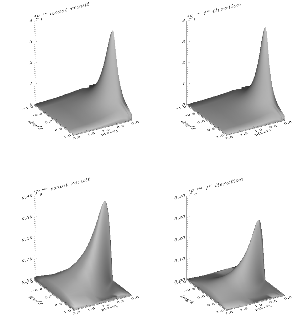
FIG. 2.: Deuteron wave function for the scalar model; exact results (left two figures) with $1^{st}$-iteration (right two figures) for ${}^{3}S_{1}^{++}$ (upper two figures) and ${}^{3}P_{1}^{o}$ (lower two figures).

FIG. 3.: Nucleon electromagnetic form factors for the nonrelativistic pair current contribution as discussed in the text. Solid line $F_{1}^{(V)}(q^{2})$, dotted line $G_{E}^{(V)}(q^{2})$, and dashed line $H(q^{2})$ as given through the Bethe-Salpeter approach.

FIG. 4.: Impulse approximation (ia, solid lines) and $\pi$-meson pair-current contributions (pc) of the differential cross section. a-c) different sets of hadronic form factors as explained in the text. Dashed line: ia+pc with $F_{1}^{(V)}(q^{2})$, dotted line: ia+pc with $H(q^{2})$, long dashed line: ia+pc with $G_{E}^{(V)}(q^{2})$. d) Calculations using $F_{1}^{(V)}(q^{2})$ only but different hadronic form factor sets as given in the text. Dashed line: ia+pc with set a, dotted line: ia+pc with set b, and long dashed line: ia+pc with set c.

REFERENCES

• [1] A. Cambi, B. Mosconi, and P. Ricci, Phys. Rev. Lett 48, 462 (1982).
• [2] M. van der Schaar et al., Phys. Rev. Lett. 68, 776 (1992), Phys. Rev. Lett. 66, 2855 (1991).
• [3] G.I. Lykasov, Phys. Part. Nucl. 24, 59 (1993) (Fiz. Elem. Chastits At. Yadra 24, 140 (1993)).
• [4] L.P. Kaptari, A.Yu. Umnikov, F.C. Khanna, and B. Kämpfer, Phys. Lett. B 351, 400 (1995).
• [5] G.I. Lykasov, Proceedings of the XIII ISHEPP “Relativistic Nuclear Physics and Quantum Chromodynamics”, Dubna, 1996.
• [6] V.V.Burov, V.N. Dostovalov and S.É. Sus’kov, Sov. J. Nucl. Phys. 23, 317 (1992).
• [7] A.V. Shebeko, V. Kotlyar, and Yu. Mel’nik, Phys. Part. Nucl. 26, 79 (1995).
• [8] J.L. Friar, Phys. Rev. C 22, 796 (1980).
• [9] J. Adam Jr., Proc. 14th Int. Conf. on Few Body Problems, Williamsburg 1994, edited by F. Gross, AIP Conf. Proc 334, 192 (1995).
• [10] F. Ritz, H. Göller, T. Wilbois, H. Arenhövel, Phys. Rev. C 55, 2214 (1997).
• [11] B.D. Keister and W.N. Polyzou, Adv. Nucl. Phys. 20, 225 (1991).
• [12] N.K. Devine and S.J. Wallace, Phys. Rev. C 48, R973 (1993).
• [13] J. Tjon, Proceedings of the 14th Int. Conf. on Few Body Problems, Williamsburg 1994, edited by F. Gross, AIP Conf. Proc 334, 177 (1995).
• [14] D. Lurie, Particles and Fields (Interscience Publishers, New York, 1968).
• [15] C. Itzykson, J.-B. Zuber, Quantum Field Theory (McGraw-Hill, Singapore 1985).
• [16] N. Nakanishi, Prog. Theor. Phys. (Kyoto) Suppl. 43, 1 (1969).
• [17] A. Yu. Umnikov, L.P. Kaptari, K.Yu. Kazakov, and F.C. Khanna, Phys. Lett. B 334, 163 (1994).
• [18] T. Nieuwenhuis, J.A.Tjon, Few-Body Syst. 21 167 (1996).
• [19] Umnikov A.Yu., Z. Phys. A 357, 333 (1997).
• [20] H. Arenhövel, Lecture Notes in Physics, Vol. 426, eds L. Mathelitsch and W. Plessas (1995) p 1.
• [21] S. Auffret et al., Phys. Rev. Lett. 55 1362 (1985); R.G. Arnold et al., Phys. Rev. C 42, R1 (1990).
• [22] J.A. Lock and L.L. Foldy, Ann. of Phys. 93, 276 (1975).
• [23] J.-F. Mathiot, Nucl. Phys. A412, 201 (1984).
• [24] S.K. Singh, W. Leidemann, H. Arenhövel, Z. Phys. A 331, 509 (1988).
• [25] W. Leidemann, and H. Arenhövel, Z. Phys. A 326, 333 (1987).
• [26] R. Schiavilla, and D.O. Riska, Phys. Rev. C 43, 437 (1991).
• [27] B. Desplanques, V.A. Karmanov, and J.-F. Mathiot, Nucl. Phys. A589, 697 (1995); J. Carbonell, B.Desplanques, V.A. Karmanov, and J.-F. Mathiot, Phys. Rep. to be published.
• [28] Kaptari L.P., Umnikov A.Yu., S.G. Bondarenko, K.Yu. Kazakov, F.C. Khanna, and Kämpfer B., Phys. Rev. C 54, 986 (1996).
• [29] J. Adam Jr., A. Stadler, M.T. Pena, and F. Gross, Nucl. Phys. A 631 570c (1998); S. Wallace ibid. 137c.
• [30] S.G. Bondarenko, V.V. Burov, M. Beyer, and S.M. Dorkin, MPG-VT-UR 87/96, e-Print Archive: nucl-th/9612047.
• [31] J.J. Kubis, Phys. Rev. 6, 547 (1972).
• [32] M.J. Zuilhof and J.A. Tjon, Phys. Rev. C 22, 2369 (1980).
• [33] V.V. Burov, A.A. Goy, S.Eh. Sus’kov, and Yu.V. Chubov, Sov. J. Nucl. Phys. 59, 989 (1996).
• [34] J.F. Mathiot, Nucl.Phys. A412, 201 (1984).
• [35] G. Höhler et al., Nucl. Phys. B114, 29 (1976).
• [36] R. Machleidt, K. Holinde, and Ch. Elster, Phys.Rep. 149, 1 (1987).
• [37] M. Gari and U. Kaulfuss, Nucl. Phys. A408, 507 (1983).
• [38] V.V. Burov, V.N. Dostovalov, and S.Eh.Sus’kov, Czech. J. of Phys. 41, 1139 (1991).
• [39] M. Lacombe et al., Phys.Rev. C21, 861 (1980).
D: $K,{\cal M}$np: $P=K+q$ $q$ $k_{e}$ $k_{e}^{\prime}$