Damping of giant resonances in asymmetric nuclear matter

Abstract

The giant collective modes in asymmetric nuclear matter are investigated within a dynamic relaxation time approximation. We derive a coupled dispersion relation and show that two sources of coupling appear: (i) a coupling of isoscalar and isovector modes due to different mean-fields acting and (ii) an explicit new coupling in asymmetric matter due to collisional interaction. We show that the latter one is responsible for a new mode arising besides isovector and isoscalar modes.

1 Theoretical Preliminaries

The treatment of collective modes in nuclear matter is documented in an enormous literature [1]. We want to investigate the collective excitations in asymmetric nuclear matter [2, 3]. To this end we like to focus on the simplest microscopic theory which provides basic experimental features. This will be accomplished by a Fermi-gas model including dissipation. We consider the system consisting of a number of different species (neutrons, protons, etc…) interacting with the own specie and with other ones. It is important to consider the interaction between different sorts of particles if we want to include friction between different streams of isospin components, etc. Especially the isospin current may not be conserved by this way. Let us start with a set of coupled quantum kinetic equations for the reduced density operator $\rho_{a}$ for a specie $a$

$$\partial_{t}\rho_{a}(t)=i[\rho_{a},{\cal E}_{a}+{\cal U}(t)_{a}]-\sum\limits_{b}\int\limits_{0}^{t}dt^{\prime}{\rho_{a}(t^{\prime})-\tilde{\rho}_{b}(t^{\prime})\over\tau_{ab}(t-t^{\prime})}$$ (1)

where ${\cal E}={\cal P}^{2}/2m$ denotes the kinetic energy operator and ${\cal U}$ the mean field operator and the external field which is assumed to be a nonlinear function of the density. We approximate the collision integral by a non-markovian relaxation time. This turned out to be necessary to reproduce damping of zero sound [5, 6]. It accounts for the fact that during a two-particle collision a collective mode can couple to the scattering process. Consequently, the dynamical relaxation time represents the physical content of a hidden three-particle process and is an equivalent to the memory effects. Further we assumed a relaxation with respect to a local equilibrium which we specify by a small deviation of the chemical potential of specie $a$ determined by current conservation. Linearizing the kinetic equation (1) we obtain the matrix equation for the density deviation $\bar{n}_{b}$ with respect to an external perturbation $U^{b}_{\rm ext}$

$$\sum\limits_{b}\bar{n}_{b}\left\{\delta_{ab}-{i\over\omega\tau_{a}+i}\left[\delta_{ab}-{\tau_{a}\over\tau_{b}}C_{ab}\right]-\Pi_{a}(\omega+{i\over\tau_{a}})\alpha_{ab}\right\}=\Pi_{a}(\omega+{i\over\tau_{a}})U_{\rm ext}^{a}.$$ (2)

The matrix $C_{ab}$ is given by

$$C_{ab}=\sum\limits_{c}\left\{1\over\tau\right\}_{ac}{\Pi_{c}\Big{[}(\omega+{i\over\tau_{a}})\frac{m_{a}}{m_{c}}\Big{]}\over\Pi_{c}(0)}\left\{\frac{1}{\tau}\right\}^{-1}_{cb}$$ (3)

with $\alpha_{ab}={\partial\over\partial\,n_{b}}\bar{U}_{a}$ the linearization of the mean field with respect to the deviation of density from equilibrium value caused by the external perturbation $U_{\rm ext}$. The partial polarization function of a specie $a$ is

$$\Pi_{a}(\omega)=2\int{dp\over(2\pi)^{3}}\frac{f_{a}(p+\frac{q}{2})-f_{a}(p-\frac{q}{2})}{\epsilon_{a}(p+\frac{q}{2})-\epsilon_{a}(p-\frac{q}{2})-\omega}.$$ (4)

The factor 2 in front of the integral accounts for the spin degeneracy according to $n_{a}=2\int{dp\over(2\pi)^{3}}f_{a}(p)$.

Equation (2) represents the complete polarization of the system, because $\bar{n}=\Pi\,U_{\rm ext}$. It represents a matrix equation which is solved easily. The collective modes are given by the zeros of the determinant of the matrix on the left hand side of (2) because these are the poles of the polarization matrix. Since we took into account relaxation processes between all species we are able to cover current - current friction. For a two component system, e.g. neutrons with density $n$ and protons with density $p$, we write explicitly

$$(1-\Pi_{n}^{\rm M}\alpha_{nn})(1-\Pi_{p}^{\rm M}\alpha_{pp})-(D_{np}+\Pi_{n}^{\rm M}\alpha_{np})(D_{pn}+\Pi_{p}^{\rm M}\alpha_{pn})=0$$ (5)

with the generalization of the Mermin polarization function [7] to a multicomponent system

$$\Pi_{a}^{\rm M}={\Pi_{a}(\omega+{i\over\tau_{a}})\over 1-{i\over\omega\tau_{a}+i}(1-C_{aa})},$$ (6)

and the additional coupling due to asymmetry in the system

$$D_{np}={\tau_{n}\over\tau_{p}}{C_{np}\over C_{nn}-i\omega\tau_{n}}.$$ (7)

The $D_{pn}$ are given by interchanging sort indices. This term does not appear for symmetric matter. Therefore we call this term asymmetry coupling term further-on.

It is illustrative to see known results for symmetric nuclear matter. This is performed for the case of equal relaxation times $\tau_{p}=\tau_{n}=\tau$ and equal deviation from the mean field $\alpha_{1}=\alpha_{nn}=\alpha_{pp}$ and $\alpha_{2}=\alpha_{np}=\alpha_{pn}$. From (5) the known Mermin result of dispersion relation [7] is then obtained

$$1-(\alpha_{1}\pm\alpha_{2}){\Pi(\omega+{i\over\tau})\over 1-{i\over\omega\tau+i}\left[1-{\Pi(\omega+{i\over\tau})\over\Pi(0)}\right]}=0$$ (8)

with the isovector mode $\alpha_{1}-\alpha_{2}$ and the isoscalar mode $\alpha_{1}+\alpha_{2}$.

We have presented a general dispersion relation for the multicomponent system including all known special cases. The dispersion relation (5) is similar to the one derived recently in [8] if we neglect the collisional coupling $D_{np}$. Also a more general polarization function (6) is presented here including collisions within a conserving approximation [9]. In the following we will apply this expression for the damping of giant dipole resonances for symmetric as well as for asymmetric nuclear matter.

2 Model for nuclear matter situation

We connect the wave vector for giant resonances according to the the Steinwedel-Jensen [10] model with the nuclear radius. If we assume that the density oscillation obeys a wave equation we get for the boundary condition that the radial velocity vanishes on the spherical surface with radius $R=1.13A^{1/3}$ such that $j_{l}^{\prime}(kR)\equiv 0$ with the spherical Bessel function of order $l=0,1...$ associated with the monopole, dipole… resonances.

Since monopole modes are compression modes we have no zero of first order for $l=0$. For the dipole modes one has in first order $k=2.08/R$ which describes the giant isovector dipole resonance (IVGDR) while the ISGDR is a spurious mode in first order. This would just mean an unphysical oscillation of center of mass motion. However, in second order $k=5.94/R$ the isoscalar giant dipole resonance (ISGDR) has been observed recently [11] and citations therein. This can be considered as a density oscillation inside a sphere. The resulting wave vectors have very low values compared with the Fermi wave vector. This allows us to expand the Mermin polarization function (6) with respect to small $qv_{c}/\omega$ ratios and $v_{c}$ the sound velocity. We obtain

$$\Pi_{a}^{\rm M}(\omega) = \frac{n_{a}(\mu_{a})}{m_{a}}{q^{2}\over\omega(\omega+{i/\tau_{a}})},$$ (9)

$$n_{a}(\mu_{a}) = 2\,\lambda_{a}^{-3}f_{3/2}(z_{a})\zeta_{corr}$$ (10)

where the thermal wave length is $\lambda_{a}^{2}=2\pi\hbar^{3}/(m_{a}T)$, $f_{3/2}$ the standard Fermi integral and $z_{a}={\rm e}^{\mu_{a}/T}$ the fugacity. The correction constant $\zeta_{corr}=1.22$ is introduced to fit the numerical solution of the dispersion relation with the approximative expansion (9). With the help of this expansion the dispersion relation (5) takes the form

$$0 = \bigg{[}\omega\Big{(}\omega+\frac{i}{\tau_{n}}\Big{)}-c_{nn}^{2}q^{2}\bigg{]}\bigg{[}\omega\Big{(}\omega+\frac{i}{\tau_{p}}\Big{)}-c_{pp}^{2}q^{2}\bigg{]}$$ (11)

$$\!\!\!-\left[c_{np}^{2}+i{\tilde{c}_{np}^{2}\over(\omega+{i/\tau_{n}})\tau_{p}}\right]\left[c_{pn}^{2}+i{\tilde{c}_{pn}^{2}\over(\omega+{i/\tau_{p}})\tau_{n}}\right]q^{4}$$

with the partial sound velocities $c$ and $\tilde{c}$

$$c_{ab}^{2}=\alpha_{ab}\frac{n_{a}(\mu_{a})}{m_{a}},\qquad\tilde{c}_{ab}^{2}=\frac{T}{m_{a}}\frac{\frac{f_{3/2}(z_{a})}{f_{1/2}(z_{a})}-\frac{f_{3/2}(z_{b})}{f_{1/2}(z_{b})}}{\frac{\tau_{ab}}{\tau_{bb}}-\frac{\tau_{aa}}{\tau_{ba}}}.$$ (12)

The dynamic relaxation time has been derived via Sommerfeld expansion [2] as

$${1\over\tau_{ab}(\omega)} = {1\over\tau_{ab}(0)}\left[1+\frac{3}{4}\left({\omega\over\pi T}\right)^{2}\right]$$ (13)

for $a,b$ neutrons or protons respectively. The markovian relaxation time was given in terms of the cross section $\sigma_{ab}$ between specie $a$ and $b$ as $\tau^{-1}_{ab}={4m\over 3\hbar^{3}}\sigma_{ab}T^{2}$. The dispersion relation (5) takes then the form of a polynomial of tenth (sixth) order corresponding to the inclusion of memory (in)dependent relaxation times. While most of these solutions will just lead to parasitary solutions (${\rm Re}\,\omega\leq 0$) we will get two coupled modes, i.e. the isoscalar and isovector mode. Furthermore a third mode appears at extreme asymmetries and/or strong collisional coupling.

The damping rate in classical approximation is given by the solution of (8) with (9) (long wavelength) and reads $\gamma=1/(2\tau)$ . We recognize that the FWHM is just twice the damping rate $\Gamma=2\gamma$. This has been recently emphasized [12]. It has to be stressed that the experimental data are accessible by this FWHM.

We will use as an illustrative example the following mean field parameterization of Vautherin [13, 14]

$$U_{a}=t_{0}\left[(1+{x_{0}\over 2})(n_{n}+n_{p})-(x_{0}+\frac{1}{2})n_{a}\right]+{t_{3}\over 4}\left[(n_{n}+n_{p})^{2}-n_{a}^{2}\right]$$ (14)

with $a=n,p$ the density of neutrons or protons respectively. The Coulomb interaction leads to an additional contribution for the proton mean-field

$$U_{p}^{C}(q)={4\pi e^{2}\over q^{2}}n_{p}(q).$$ (15)

The here used model parameters reproduce the Weizsäcker formula

$${E\over A}=-a_{1}+{a_{2}\over A^{1/3}}+{a_{3}Z^{2}\over A^{4/3}}+a_{4}\delta^{2}$$ (16)

by the volume energy $a_{1}=15.68$ MeV, Coulomb energy $a_{3}=0.717$ MeV and the symmetry energy $a_{4}=28.1$ MeV with the asymmetry parameter $\delta={n_{n}-n_{p}\over n_{n}+n_{p}}$.

First we plot the solution of the dispersion relation (11) for symmetric nuclear matter. In figure 2 we plotted the real and imaginary (FWHM) part of complex energy for different approximations with relaxation time (collisions) with and without Coulomb. In [figure 2 (A)] we find that the inclusion of Coulomb effects reproduces the experimental shape of the centroid energies at higher mass numbers (dot-dashed line). Taking only collisions into account fails to describe higher mass numbers (solid line). Considering Coulomb together with collisions (dashed line), the centroid energies are reduced towardes the data.

The experimental values of the damping rates are also presented versus mass number [figure 2 (B)]. Without collisions we would only have a vanishing Landau damping for the infinite matter model [2]. We see that the inclusion of Coulomb (dashed line) improves the situation.

Figure 1: The experimental centroid energies (A) and damping rates (B) [filled symbols] of the giant dipole resonances vs mass number (data from Ref. [15]) together with different approximations at $T=0$.

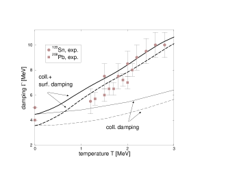
Figure 2: The effective damping consisting of only collisional damping compared with collisional and surface damping [¹²⁰Sn (solid lines) and ²⁰⁸Pb (dashed lines)] together with the experimental data (filled symbols: Sn from Ref. [16] and Pb from Ref. [17]).

The failure of the considered processes becomes more drastic if we consider the temperature dependence of the GDR. In figure 2 we see that the temperature increase is too flat compared to the experimental finding if we consider only collisional damping (thin lines). In Ref. [18] we present a method to include also scattering with the nuclear surface. This improves the temperature dependence remarkably (thick lines).

Isoscalar giant dipole resonances (ISGDR) are observed recently in ${}^{208}Pb$ [11] and are given with a value

$$E^{\rm ex}_{\rm ISGDR}=22.4\pm 0.5\,{\rm MeV},\qquad\Gamma^{\rm ex}_{\rm ISGDR}=3.0\pm 0.5\,{\rm MeV}.$$ (17)

They can be considered as a density oscillation inside a sphere. We obtain with the model parameters of IVGDR and a corresponding second order in $j_{l}^{\prime}(kR)=0$

$$E_{\rm ISGDR}=21.0\,{\rm MeV},\qquad\Gamma_{\rm ISGDR}=3.4\,{\rm MeV}$$ (18)

which is quite acceptable and is in the middle of different theoretical treatments ([11] and citations therein).

3 New collective mode

Now we employ the same potential as in the last section but assume different neutron and proton densities. In figure 3 we plot the isoscalar and isovector modes versus temperature for ${}^{48}Ca$ with a small asymmetry $\delta=0.2$ as well as for ${}^{60}Ca$ with a asymmetry $\delta=0.33$. The kinetic energy is linked to a temperature within the Fermi liquid model via Sommerfeld expansion

$${E\over A} = \frac{3}{5}\epsilon_{f}\left[{(1+\delta)^{5/3}+(1-\delta)^{5/3}\over 2}\right.+\left.{5\over 12}\pi^{2}\left({T\over T_{f}}\right)^{2}{(1+\delta)^{1/3}+(1-\delta)^{1/3}\over 2}\right].$$ (19)

This connection between temperature and excitation energy is only valid for a continuous Fermi liquid model. For the small nuclei, the concept of temperature is questionable. Some improvement one can obtain by the definition of temperature via the logarithmic derivative of the density of states [19]

$$T^{-1}=\frac{1}{\rho}{\partial\rho\over\partial E_{\rm ex}}=-\frac{5}{4}E_{\rm ex}^{-1}+\pi({A\over 4\epsilon_{f}E_{\rm ex}})^{1/2}$$ (20)

which provides $E_{\rm ex}\approx\frac{1}{4}(E/A)$ in comparison with (19) for small temperatures. We use this temperature to demonstrate possible collective bulk features in an exploratory sense. Of course, the surface energy and shell effects cannot be neglected for realistic calculations.

With increasing temperature the isovector and isoscalar energies decrease and vanish at a certain temperature. At these temperatures the damping becomes twofold because the damping of the spurious mode with negative energy becomes different from the physical mode. We can consider this behavior of damping as a phase transition of isospin demixture.

At the same time a very soft mode appears due to collisional coupling which is only present in asymmetric matter [20]. This mode is more pronounced in the next figure 3 for ${}^{60}Ca$ with an asymmetry of $\delta=0.33$.

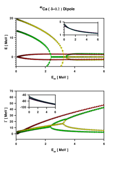
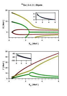
Figure 3: The energy and damping of the IVGDR and ISGDR of ${}^{48}Ca$ (left) and ${}^{60}Ca$ (right) vs excitation energy. Besides the isovector modes (circles) and the isoscalar modes (squares) a soft third mode appears (triangles).

We see that the isovector mode does not disappear but turns over into a flat decrease with increasing temperature. This behavior is coupled with the pronounced soft mode. In comparison with the more symmetric ${}^{48}Ca$ we see a different behavior of the damping where the isoscalar mode vanishes. Also the isovector mode appears unique and not two-folded. Now a clear transition of damping behavior for the isovector mode is recognizable which can be considered as a transition from zero to first sound damping.

4 Summary

To summarize we have observed that due to correlational coupling there can exist a new mode which appears besides isovector and isoscalar modes in asymmetric nuclear matter due to collisions. We suggest that this mode may be possible to observe as a soft collective excitation in asymmetric systems. The transition from zero sound damping to first sound damping behavior should become possible to observe for isovector modes since they do not vanish at this transition temperature like in symmetric matter.

The authors thank for the fruitful discussions with M. DiToro, A. Larionov and V. Baran. The hospitality of LNS-INFN Catania where part of this work has been finished, is gratefully acknowledged. The work was supported by the Max-Planck Society Germany.

References

- [1] J.C. Bacelar and M.N. Harakeh and O. Scholten, Proceedings of the Groningen conference on giant resonances, Nucl. Phys. A 599, 1 (1996).
- [2] U. Fuhrmann, K. Morawetz, and R. Walke, Phys. Rev. C 58, 1473 (1998).
- [3] F. Catara, E. G. Lanza and M. A. Nagarajan and A. Vitturi, Nucl. Phys. A 624, 449 (1996).
- [4] G. Fabbri and F. Matera, nucl-th/9805022.
- [5] S. Ayik and D. Boilley, Phys. Lett. B 276, 263 (1992), errata ibd. 284 (1992) 482.
- [6] K. Morawetz, M. DiToro, and L. Münchow, Phys. Rev. C 54, 833 (1996).
- [7] N. D. Mermin, Phys. Rev. B 1, 2362 (1970).
- [8] M. Colonna, M. DiToro, and A. B. Larionov, Phys. Rev. Lett. (1997), sub., Preprint LNS16-05-97.
- [9] H. Heiselberg, C. J. Pethick, and D. G. Ravenhall, Ann. Phys. 223, 37 (1993).
- [10] H. Steinwedel and J. Jensen, Z. f. Naturforschung 5, 413 (1950).
- [11] B. Davis et al., Phys. Rev. C (1998), sub..
- [12] M. Di Toro, V. Kolomietz, and A. Larionov, in proceedings of the Dubna conference on heavy ions (unpublished, Dubna, 1997).
- [13] D. Vautherin and D. M. Brink, Phys. Rev. C 5, 626 (1972).
- [14] F. Braghin and D. Vautherin, Phys. Lett. B 333, 289 (1994).
- [15] S. Dietrich and B. Berman, Nucl. Data Tabl. 38, 199 (1988).
- [16] E. Ramkrishnan et al., Phys. Rev. Lett. 76, 2025 (1996).
- [17] E. Ramkrishnan et al., Nucl. Phys. A 549, 49 (1996).
- [18] K. Morawetz, M. Vogt, U. Fuhrmann, V. Špička and P. Lipavský, Phys. Rev. C (1998), sub..
- [19] A. Bohr and B. R. Mottelson, Nuclear Structure (W. A. Benjamin, Inc., New York, 1969).
- [20] K. Morawetz, R. Walke, U. Fuhrmann and M. DiToro, Phys. Rev. C 57, 2813 (1998).