DOE/ER/40561-28-INT98
TRI-PP-98-17
KRL MAP-235
NT@UW-98-24
Renormalization of the Three-Body System with Short-Range Interactions

Abstract

We discuss renormalization of the non-relativistic three-body problem with short-range forces. The problem becomes non-perturbative at momenta of the order of the inverse of the two-body scattering length, and an infinite number of graphs must be summed. This summation leads to a cutoff dependence that does not appear in any order in perturbation theory. We argue that this cutoff dependence can be absorbed in a single three-body counterterm and compute the running of the three-body force with the cutoff. We comment on relevance of this result for the effective field theory program in nuclear and molecular physics.

Systems composed of particles with momenta $k$ much smaller than the inverse range $1/R$ of their interaction are common in nature. This separation of scales can be exploited by the method of effective field theory (EFT) that provides a systematic expansion in powers of the small parameter $kR$ [1]. Generically, the two-body scattering length $a_{2}$ is comparable to $R$, and low-density systems with $k\ll 1/a_{2}$ can be described to any order in $kR$ by a finite number of EFT graphs [2]. However, there are many interesting systems, such as those made out of nucleons or of ⁴He atoms, for which $a_{2}$ is much larger than $R$. In this case the expansion becomes non-perturbative at momenta of the order of $1/a_{2}$, in the sense that an infinite number of diagrams must be resummed. This resummation generates a new expansion in powers of $kR$ where the full dependence in $ka_{2}$ is kept. Consequently, the EFT is valid beyond $k\sim 1/a_{2}$, comprising, in particular, bound states of size $\sim a_{2}$. There has been enormous progress recently in dealing with this problem in the two-body case [3], where the resummation is equivalent to effective range theory [4]. Ultraviolet (UV) divergences appear in graphs with leading-order interactions and their resummation contains arbitrarily high powers of the cutoff. A crucial point is that this cutoff dependence can be absorbed in the coefficients of the leading-order interactions themselves. All our ignorance about the influence of short-distance physics on low-energy phenomena is then embodied in these few coefficients, and EFT retains its predictive power. However, the extension of this program to three-particle systems presents us with a puzzle [5]. Although in some fermionic channels the resummed leading two-body interactions lead to unambiguous and very successful predictions [6, 7], amplitudes in bosonic systems and other fermionic channels show sensitivity to the UV cutoff, as evidenced in the Thomas [8] and Efimov [9] effects. This happens even though each leading-order three-body diagram with resummed two-body interactions is individually UV finite. We will argue below that the addition of a one-parameter three-body force counterterm at leading order is necessary and sufficient to eliminate this cutoff dependence. This result extends the EFT program to three-particle systems with large two-body scattering lengths, including the approach of Ref. [10] where pions are treated perturbatively.

The most general Lagrangian involving a non-relativistic boson $\psi$ and invariant under small-velocity Lorentz, parity, and time-reversal transformations is

$${\cal L}=\psi^{\dagger}(i\partial_{0}+\frac{\vec{\nabla}^{2}}{2M})\psi-\frac{C_{0}}{2}(\psi^{\dagger}\psi)^{2}-\frac{D_{0}}{6}(\psi^{\dagger}\psi)^{3}+\ldots,$$ (1)

where the ellipsis denote terms with more derivatives and/or fields; those with more fields will not contribute to the three-body amplitude, while those with more derivatives are suppressed at low momentum. It is convenient [11] to rewrite this theory by introducing a dummy field $T$ (called “dibaryon” in analogy to the nuclear case) with quantum numbers of two bosons,

$${\cal L} = \psi^{\dagger}(i\partial_{0}+\frac{\vec{\nabla}^{2}}{2M})\psi+\Delta T^{\dagger}T-\frac{g}{\sqrt{2}}(T^{\dagger}\psi\psi+\mbox{h.c.})$$ (2)

$$+ hT^{\dagger}T\psi^{\dagger}\psi+\ldots$$ (3)

The arbitrary scale $\Delta$ is included to give the field $T$ the usual mass dimension. Observables depend on the parameters of Eq. (2) only through the combinations $C_{0}\equiv g^{2}/\Delta=4\pi a_{2}/M$ and $D_{0}\equiv-3hg^{2}/\Delta^{2}$. The (bare) dibaryon propagator is simply a constant $i/\Delta$, while the particle propagator reduces to the usual non-relativistic form $i/(p^{0}-p^{2}/2M)$. First, we consider the dressing of the dibaryon in Fig. 1(a) at a generic momentum $Q$. The boson loop has a linear UV divergence that is absorbed in $g^{2}/\Delta$, a finite piece $\sim Mg^{2}Q/4\pi\Delta^{2}$ determined by the unitarity cut, and terms suppressed by powers of $Q$ over the cutoff $\Lambda$ that are subleading and of the same size as terms in Eq. (2) already disregarded. Using the relation between $g$ and $a_{2}$, we see that the finite piece is $\sim Qa_{2}/\Delta$ and, consequently, has to be resummed to all orders for $Q\hskip 1.99997pt\raisebox{2.15277pt}{$>$}\raisebox{-3.00003pt}{$\sim$}\hskip 1.99997pt1/a_{2}$. As a result, the dressed dibaryon propagator to leading order is given by

$$iS(p)=\frac{1}{-\Delta+\frac{Mg^{2}}{4\pi}\sqrt{-Mp^{0}+\frac{\vec{p}^{\,2}}{4}-i\epsilon}+i\epsilon}.$$ (4)

Attaching four boson lines to this propagator gives the two-particle scattering amplitude at leading order, which is identical to the effective range expansion at the order of the scattering length. Further corrections give the next terms in the effective range expansion [4].

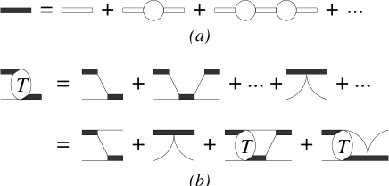
FIG. 1.: (a) Dressing of the dibaryon. (b) Diagrams contributing to particle/bound-state scattering.

Let us now consider particle/bound-state scattering. All diagrams contributing to this process in leading order are illustrated in Fig. 1(b). Each of the diagrams including only two-body interactions gives a contribution of order $\sim Mg^{2}/Q^{2}\sim 4\pi\Delta a_{2}^{3}$. (The properly normalized amplitude is independent of the arbitrary parameter $\Delta$; it appears here only because of our choice of interpolating field for the bound state.) The relative size of graphs that include a three-body force will be discussed shortly.

The sum of all the diagrams in Fig. 1(b) can be accomplished by solving the equation represented by the second equality in Fig. 1(b) [5, 6, 7, 12]:

$$a(p)=K(p,k)+\frac{2\lambda}{\pi}\int_{0}^{\Lambda}dq\ K(p,q)\frac{q^{2}}{q^{2}-k^{2}-i\epsilon}a(q),$$ (5)

where $k$ ($p$) is the incoming (outgoing) momentum, $ME=3k^{2}/4-1/a_{2}^{2}$ is the total energy, $a(p=k)$ is the scattering amplitude normalized in such a way that $a_{3}=-a(0)$ is the particle/bound-state scattering length, and

$$K(p,q)=\frac{4}{3} (\frac{1}{a_{2}}+\sqrt{\frac{3}{4}p^{2}-ME})$$ (7)

$$\left[\frac{1}{pq}{\rm ln}\left(\frac{q^{2}+pq+p^{2}-ME}{q^{2}-qp+p^{2}-ME}\right)+\frac{h}{Mg^{2}}\right].$$

The parametric dependence of $a(p)$ on $k$ is kept implicit. We are interested in $\lambda=1$ for the boson case. This equation reduces to the expressions found in Ref. [5, 12] when $h=0$. Three nucleons in the spin $J=1/2$ channel obey a pair of integral equations with similar properties to this bosonic equation, while the spin $J=3/2$ channel corresponds to $\lambda=-1/2$.

Let us look at the asymptotic behavior of the solution of Eq. (5) in the case $h=0$. For $1/a_{2}\ll p\ll\Lambda$ (but $k\sim 1/a_{2}$), the integral in Eq. (5) is dominated by momenta in the intermediate region $1/a_{2}\ll q\ll\Lambda$ and the equation

$$a(p)=\frac{4\lambda}{\sqrt{3}\pi}\int_{0}^{\infty}\>\frac{dq}{q}\ a(q)\,{\rm ln}\left(\frac{q^{2}+pq+p^{2}}{q^{2}-pq+p^{2}}\right),$$ (8)

holds up to terms suppressed by powers of $1/pa_{2}$ and/or $p/\Lambda$. The scale invariance of Eq. (8) suggests an ansatz of the form $a(p)\sim p^{s}$, which works if $s$ satisfies

$$1-\frac{8\lambda}{\sqrt{3}}\frac{\sin\frac{\pi s}{6}}{s\cos\frac{\pi s}{2}}=0.$$ (9)

The solutions of Eq. (9) come in pairs due to the additional symmetry $a(p)\rightarrow a(1/p)$ of Eq. (8). For $\lambda<\lambda_{c}={3\sqrt{3}\over 4\pi}\simeq 0.4135$, Eq. (9) has only real roots. However, for $\lambda=1$ there are two imaginary solutions $s=\pm is_{0}$, with $s_{0}\simeq 1.0064$. Both make the integral in Eq. (5) UV finite and are equally acceptable: $a(p)$ is given in the intermediate region by a linear combination of $p^{is_{0}}$ and $p^{-is_{0}}$. Eq. (8) is homogeneous so it clearly cannot determine the overall normalization of $a$, but we now see that it cannot uniquely determine the phase either. However, Eq. (8) with finite $\Lambda$ has a solution with a well determined phase that in the intermediate region $1/a_{2}\ll p\ll\Lambda$ is, on dimensional grounds,

$$a(p)=A\cos(s_{0}\ln\frac{p}{\Lambda}+\delta),$$ (10)

where $\delta$ is some dimensionless, cutoff-independent number. The limit $\Lambda\rightarrow\infty$ is not well defined because Eq. (5) does not have a unique solution in this limit. (A rigorous proof that Eq. (5) does not have a unique solution can be found in [13].) This non-uniqueness comes from our idealization of the interactions as point-like. Note that subleading contributions from the integration range $\Lambda\leq q\leq\infty$ change phase and amplitude significantly. Numerical solutions of Eq. (5) with $k=0$ for different values of $\Lambda$ are plotted in Fig. 2. (Our results agree with those in Ref. [14] for the appropriate cutoff values.) We observe that indeed the behavior of $a(p)$ in the region $1/a_{2}\ll p\ll\Lambda$ is given by Eq. (10) and that small differences in the asymptotic phase lead to large differences in the particle/bound-state scattering length.

FIG. 2.: $a(p)$ for $k=0$. Full, dashed, and dash-dotted curves are for $H=0$ and $\Lambda=1.0,\,2.0,\,3.0\times 10^{4}a_{2}^{-1}$, respectively. Dotted, short-dash-dotted, and short-dashed curves are for $\Lambda=10^{4}a_{2}^{-1}$ and $H=-6.0,\,-2.5,\,-1.8$, respectively.

Note that if the series of diagrams in Fig. 1(b) was truncated at some finite number of loops one would miss the correct asymptotic behavior of $a(p)$ (Eq. (10)) that generates the cutoff dependence. This is because $s_{0}$ (and its expansion in powers of $\lambda$) vanish in a neighborhood of $\lambda=0$ and the truncation of the series in Fig. 1(b) is equivalent to perturbation theory in $\lambda$.

This cutoff dependence comes from the behavior of the amplitude in the UV region, where the EFT Lagrangian, Eq. (2), is not to be trusted. When the low-energy expansion is perturbative, the cutoff-dependent contribution from high loop momenta can be expanded in powers of the low external momenta and cancelled by local terms in the Lagrangian. Thus all uncertainty coming from the high momentum behavior of the theory is parametrized by a few local counterterms. The present case is complicated by the non-analytic cutoff dependence of the amplitude around $p=0$. That, however, does not mean that the renormalization program is doomed: a three-body force term of sufficient strength contributes not only at tree level, but also in loops dressed by any number of two-particle interactions. This generates non-local contributions precisely of the same form as the cutoff-dependent terms generated by the two-body force alone. To see how that comes about we turn on the three-body force term and write $h(\Lambda)=2Mg^{2}H(\Lambda)/\Lambda^{2}$ assuming $H(\Lambda)\sim 1$. The asymptotic Eq. (8) becomes

$$a(p)=\frac{4}{\sqrt{3}\pi}\int_{0}^{\Lambda}\>\frac{dq}{q}\ a(q)\left[{\rm ln}\left(\frac{q^{2}+pq+p^{2}}{q^{2}-pq+p^{2}}\right)+2H\frac{pq}{\Lambda^{2}}\right],$$ (11)

where we have set $\lambda=1$ for definiteness. For $p\sim\Lambda$ the term proportional to $H$ becomes important and $a(p\sim\Lambda)$ has a complicated form. In the range $1/a_{2}\ll p\ll\Lambda$, however, the three-body force is suppressed by $p/\Lambda$ compared to the logarithm and can be disregarded. Consequently, Eq. (10) is still correct in the intermediate region. The effect of a finite value of $H$ can be at most to change the values of the amplitude $A$ and the phase $\delta$, which become functions of $H$. As shown in Fig. 2, this is confirmed by numerical solutions: while different values of the three-body force preserve the form of the solution, the phase (and amplitude) are changed. If $H$ is chosen to be a function of $\Lambda$ such as to cancel the explicit $\Lambda$ dependence, we can make the solution of Eq. (5) cutoff independent for all $p\ll\Lambda$. In particular the scattering amplitude that is determined by the on-shell value $a(k)$ with $k\sim 1/a_{2}$ will be cutoff independent as well. For this to be possible $A$ and $\delta$ must depend on the same combination of $\Lambda$ and $H$. Thus $H(\Lambda)$ must be chosen such that

$$-s_{0}\ln\Lambda+\delta(H(\Lambda))=-s_{0}\ln\Lambda_{\star},$$ (12)

where $\Lambda_{\star}$ is a parameter fixed by experiment or by matching with a microscopic model.

We can get a handle on the form of $H(\Lambda)$ by considering Eq. (5) with two different values of the cutoff $\Lambda$ and $\Lambda^{\prime}>\Lambda$, whose solutions we denote by $a(p)$ and $a^{\prime}(p)$. In the intermediate region $1/a_{2}\ll p\ll\Lambda$ the equations for $a(p)$ and $a^{\prime}(p)$ will have the same form except for

$$\frac{2}{\pi}\!\left[\int_{\Lambda}^{\Lambda^{\prime}}\!\!\!\!dq\,K^{\prime}(p,q)\,a^{\prime}(q)+2\!\!\int_{\mu}^{\Lambda}\!\!\!dq\left(\frac{H(\Lambda^{\prime})}{\Lambda^{\prime}}-\frac{H(\Lambda)}{\Lambda}\right)a^{\prime}(q)\right]$$ (13)

where $\mu\ll\Lambda$ is an arbitrary scale, and we dropped terms suppressed by further powers of $1/pa_{2}$ and $p/\Lambda$. Assuming $a^{\prime}(p)$ has the same phase $\cos(s_{0}\ln(p/\Lambda_{\star}))$ as $a(p)$ even for $p\sim\Lambda^{\prime}$, we can make the terms in Eq. (13) vanish by choosing

$$H(\Lambda)=-\frac{\sin(s_{0}\ln({\Lambda}/{\Lambda_{\star}})-{\rm arctg}(1/s_{0}))}{\sin(s_{0}\ln({\Lambda}/{\Lambda_{\star}})+{\rm arctg}(1/s_{0}))}.$$ (14)

Since $K^{\prime}-K$ nearly vanishes for all $p\ll\Lambda$, $a^{\prime}(p)$ has also the same amplitude as $a(p)$ in the intermediate region. That is, with $H(\Lambda)$ chosen like Eq. (14), $a(p)=a^{\prime}(p)$ for all values $p\ll\Lambda$ (up to terms suppressed by $p/\Lambda$), and the on-shell amplitude $a(k)$ for $k\ll\Lambda$ will be $\Lambda$ independent. Once the parameter $\Lambda_{\star}$ is fitted to an experimental datum at a certain energy, the energy dependence can be predicted.

We also determine $H(\Lambda)$ numerically by finding the value of $H$ that keeps the scattering length $a_{3}=-a(0)$ constant for each value of $\Lambda$ varying over a large range. These values are plotted as a function of $\Lambda$ in Fig. 3 together with $H(\Lambda)$ given by Eq. (14). For illustration we used $a_{3}=1.56a_{2}$, but have verified that similar agreement holds for other values of $a_{3}$. In Fig. 4 we show the corresponding $k\cot\delta=ik+a(k)^{-1}$, where $\delta$ is the $S$-wave phase shift for particle/bound-state scattering, for several values of $\Lambda$. As argued above, it is insensitive to $\Lambda$ as long as $k\ll\Lambda$. The effective range, for example, is predicted as $r_{3}=0.57a_{2}$. Note that the three-body force discussed here is not the one used in realistic potential models where the effective cutoff is at much higher scales.

FIG. 3.: Three-body force as a function of the cutoff $\Lambda$: numerical solution (dots) and Eq.(14).

FIG. 4.: Energy dependence: $k\cot\delta$ for different cutoffs ($\Lambda=42.6,\,100.0,\,230.0,\,959.0\times a_{2}^{-1}$).

These arguments hold for the bound-state problem as well because the inhomogeneous terms played no role. We have solved the homogeneous equation with the $H(\Lambda)$ of Fig. 3. Only the shallowest bound state is large enough to be unequivocally within the limits of applicability of the EFT; it has a cutoff-independent binding energy of $B_{3}=1.5/Ma_{2}^{2}$.

The value for the ratio $a_{3}/a_{2}$ used above is the one suggested by the values of $a_{2}=124.7$ Å and $a_{3}=195$ Å given by a phenomenological ⁴He-⁴He potential [15] consistent with the recent measurement of the dimer binding energy [16]. Fig. 4 then represents the phase shifts for atom/dimer scattering, with an effective range $r_{3}=71$ Å. Similarly, our result for the shallowest bound state suggests an excited state of the trimer at $B_{3}=1.2$ mK. Because the integral equations are similar, our arguments are relevant for three-fermion systems with internal quantum numbers as well [17]. The approach of Ref. [10] then suggests that our bound-state results would provide a reasonable estimate of the triton binding energy.

In conclusion, we have provided analytical and numerical evidence that renormalization of the three-body problem with short-range forces requires in general the presence of a one-parameter contact three-body force in leading order. This opens up the possibility of applying the EFT method to a large class of systems of three or more particles with short-range forces.

We thank V. Efimov, H. Müller, and D. Kaplan for helpful discussions. HWH acknowledges hospitality of the Nuclear Theory Group and the INT in Seattle. Research supported in part by the U.S. DOE (DOE-ER-40561 and DE-FG03-97ER41014), the NSERC of Canada, and the U.S. NSF (PHY94-20470).

REFERENCES

- [1] G.P. Lepage, in “From Actions to Answers, TASI’89”, ed. T. DeGrand and D. Toussaint, World Scientific, 1990; D.B. Kaplan, nucl-th/9506035; H. Georgi, Ann. Rev. Part. Sci. 43 (1994) 209.
- [2] E. Braaten and A.Nieto, Phys. Rev. B56 (1997) 14745; Phys. Rev. B55 (1997) 8090.
- [3] “Nuclear Physics with Effective Field Theory”, ed. R. Seki, U. van Kolck, and M.J. Savage, World Scientific, 1998.
- [4] U. van Kolck, nucl-th/9808007; and references therein.
- [5] P.F. Bedaque, in Ref. [3], nucl-th/9806041.
- [6] P.F. Bedaque and U. van Kolck, Phys. Lett. B428 (1998) 221.
- [7] P.F. Bedaque, H.-W. Hammer, and U. van Kolck, Phys. Rev. C58 (1998) R641.
- [8] L.H. Thomas, Phys. Rev. 47 (1935) 903; S.K. Adhikari, T. Frederico, and I.D. Goldman, Phys. Rev. Lett. 74 (1995) 487.
- [9] V.N. Efimov, Sov. J. Nucl. Phys. 12 (1971) 589; Phys. Rev. C47 (1993) 1876.
- [10] D.B. Kaplan, M.J. Savage, and M.B. Wise, Phys. Lett. B424 (1998) 390; nucl-th/9802075.
- [11] D.B. Kaplan, Nucl. Phys. B494 (1997) 471.
- [12] G.V. Skorniakov and K.A. Ter-Martirosian, Sov. Phys. JETP 4 (1957) 648.
- [13] G.S. Danilov and V.I. Lebedev, Sov. Phys. JETP 17 (1963) 1015;
- [14] V.F. Kharchenko, Sov. J. Nucl. Phys. 16 (1973) 173.
- [15] S. Nakaichi-Maeda and T.K. Lim, Phys. Rev. A28 (1983) 692; A.K. Motovilov, S.A. Sofianos, and E.A. Kolganova, Chem. Phys. Lett. 275 (1997) 168.
- [16] F. Luo, C.F. Giese, and W.R. Gentry, J. Chem. Phys. 104 (1996) 1151.
- [17] P.F. Bedaque, H.-W. Hammer, and U. van Kolck, in progress.