$\gamma$-Deuteron Compton Scattering in Effective Field Theory

Abstract

The differential cross section for $\gamma$-deuteron Compton scattering is computed to next-to-leading order (NLO) in an effective field theory that describes nucleon-nucleon interactions below the pion production threshold. Contributions at NLO include the nucleon isoscalar electric polarizability from its $1/m_{\pi}$ behavior in the chiral limit. The parameter free prediction of the $\gamma$-deuteron differential cross section at NLO is in good agreement with data.

I Introduction

The differential cross section for $\gamma$-deuteron Compton scattering has been measured at incident photon energies of $49\ {\rm MeV}$ and $69\ {\rm MeV}$[1]. At these energies the forward scattering amplitude is dominated by the charged proton while contributions from the strong interactions that bind the nucleons into the deuteron are suppressed by factors of the binding energy divided by the photon energy. Contributions from the structure of the nucleon are suppressed by factors of the photon energy divided by the chiral symmetry breaking scale. For finite angle scattering the deuteron size plays an important role by setting the scale of the variation of form factors. It has been suggested that a precise measurement of $\gamma$-deuteron Compton scattering will determine the isoscalar electric and magnetic nucleon polarizabilities. Given precise measurements of the proton polarizabilities this would determine the neutron polarizabilities. However, since the physics responsible for binding the deuteron has the same origin as the physics giving rise to the nucleon polarizabilities, the separation between binding effects and nucleon structure is unclear.

The nucleon electromagnetic polarizabilities measure the deformation of the nucleon in external electric and magnetic fields (for an overview see [2]). Combined analyses of $\gamma$-proton Compton scattering and photoabsorption sum rules give a proton electric polarizability of $\alpha_{E,p}=(12.1\pm 0.8\pm 0.5)\times 10^{-4}\ {\rm fm}^{3}$ and magnetic polarizability of $\beta_{M,p}=(2.1\mp 0.8\mp 0.5)\times 10^{-4}\ {\rm fm}^{3}$[3, 4]. However, the neutron polarizabilities are much more difficult to obtain. Since there is no free neutron target, either $\gamma$-deuteron Compton scattering [1, 7] or neutron scattering off heavy nuclei is used to extract the neutron polarizability[5, 6]. One extraction of the neutron electric polarizability from its characteristic influence on the energy dependence of the neutron-²⁰⁸Pb scattering cross section gave a precise value of $\alpha_{E,n}=(12.0\pm 1.5\pm 2.0)\times 10^{-4}\ {\rm fm}^{3}$ [5]. A more recent analysis gives a different central value with large uncertainty, $\alpha_{E,n}=(0\pm 5)\times 10^{-4}\ {\rm fm}^{3}$[6]. Meanwhile, quasi-free $\gamma$-deuteron Compton scattering $d(\gamma,\gamma^{{}^{\prime}}n)p$ gives a value of $\alpha_{E,n}$ consistent with zero but also with a large uncertainty $\alpha_{E,n}=(10.7_{-10.7}^{+3.3})\times 10^{-4}\ {\rm fm}^{3}$[7]. An analysis of $\gamma$-deuteron Compton scatting with a simple potential model gives values of $\alpha_{E,n}=(20\pm 6\pm 3)\times 10^{-4}\ {\rm fm}^{3}$ and $\beta_{M,p}=(10\pm 6\pm 3)\times 10^{-4}\ {\rm fm}^{3}$[1]. Calculations with more realistic potentials and interactions were performed for this process [8, 9] with the nucleon isoscalar polarizabilities input rather than treated as free parameters. A more sophisticated potential model calculation is currently being performed by Karakowski and Miller[10].

Recently, significant theoretical effort[11, 12, 13, 14, 15, 16, 17, 18, 19, 20, 21, 22, 23, 24, 25, 26, 27, 28, 29, 30, 31, 32] has produced an effective field theory with consistent power counting that describes the low-energy interactions of two nucleons. The leading contribution to two nucleons scattering in an S-wave comes from local four-nucleon operators. Contributions from pion exchanges and from higher derivative operators are suppressed by additional powers of the external nucleon momentum and by powers of the light quark masses[29, 30]. To accommodate the unnaturally large scattering lengths in S-wave nucleon nucleon scattering, fine-tuning is required. This fine-tuning can complicate power counting in the effective field theory, but dimensional regularization with power divergence subtraction (PDS), described in [29], provides a consistent power counting scheme. The technique successfully describes the $NN$ scattering phase shifts up to center-of-mass momenta of ${\bf p}\sim 300\ {\rm MeV}$ per nucleon[29] in all partial waves. The electromagnetic moments, form factors [30] and polarizability [33] of the deuteron as well as parity violation in the two-nucleon sector [34] have been explored with this new effective field theory. In this paper we perform a model independent, analytic calculation of $\gamma$-deuteron Compton scattering up to next-to-leading order (NLO) in the nucleon-nucleon effective field theory. The gauge invariant set of pion graphs that gives the dominant contribution to the electric polarizability of the nucleon contribute to $\gamma$-deuteron Compton scattering at NLO. We will not treat the polarizabilities as parameters, but instead compute the $\gamma$-deuteron Compton scattering including these pion loop graphs and show that the differential cross section is in good agreement with the data. This avoids the problem of defining “nucleon structure” in the deuteron bound-state (i.e., we only compute S-matrix elements) and means that we do not have to deal with the issue of field redefinitions (i.e., “off-shell effects”).

II Effective Field Theory for Nucleon-Nucleon Interactions

The terms in the effective Lagrange density describing the interactions between nucleons, pions, and photons can be classified by the number of nucleon fields that appear. It is convenient to write

$${\cal L}={\cal L}_{0}+{\cal L}_{1}+{\cal L}_{2}+\ldots,$$ (1)

where ${\cal L}_{n}$ contains $n$-body nucleon operators.

${\cal L}_{0}$ is constructed from the photon field $A^{\mu}=(A^{0},{\bf A})$ and the pion fields which are incorporated into an $SU(2)$ matrix,

$$\Sigma=\exp\left({{\textstyle{\displaystyle 2i\Pi\over\displaystyle f}}}\right)\ \ \ ,\qquad\Pi=\left(\begin{array}[]{cc}\pi^{0}/\sqrt{2}&\pi^{+}\\ \pi^{-}&-\pi^{0}/\sqrt{2}\end{array}\right)\ \ \ \ ,$$ (2)

where $f=132\ {\rm\ MeV}$ is the pion decay constant. $\Sigma$ transforms under the global $SU(2)_{L}\times SU(2)_{R}$ chiral and $U(1)_{em}$ gauge symmetries as

$$\Sigma\rightarrow L\Sigma R^{\dagger},\qquad\Sigma\rightarrow e^{i\alpha Q_{em}}\Sigma e^{-i\alpha Q_{em}}\ \ \ ,$$ (3)

where $L\in SU(2)_{L}$, $R\in SU(2)_{R}$ and $Q_{em}$ is the charge matrix,

$$Q_{em}=\left(\begin{array}[]{cc}1&0\\ 0&0\end{array}\right)\ \ \ .$$ (4)

The part of the Lagrange density without nucleon fields is

$${\cal L}_{0} ={1\over 2}({\bf E}^{2}-{\bf B}^{2})\ +\ {f^{2}\over 8}{\rm Tr\,}D_{\mu}\Sigma D^{\mu}\Sigma^{\dagger}\ +\ {f^{2}\over 4}\lambda{\rm Tr\,}m_{q}(\Sigma+\Sigma^{\dagger})\ +\ \ldots\ \ \ \ .$$ (5)

The ellipsis denote operators with more covariant derivatives $D_{\mu}$, insertions of the quark mass matrix $m_{q}={\rm diag}(m_{u},m_{d})$, or factors of the electric and magnetic fields. The parameter $\lambda$ has dimensions of mass and $m_{\pi}^{2}=\lambda(m_{u}+m_{d})$. Acting on $\Sigma$, the covariant derivative is

$$D_{\mu}\Sigma=\partial_{\mu}\Sigma+ie[Q_{em},\Sigma]A_{\mu}\ \ \ .$$ (6)

When describing pion-nucleon interactions, it is convenient to introduce the field $\xi=\exp\left(i\Pi/f\right)=\sqrt{\Sigma}$. Under $SU(2)_{L}\times SU(2)_{R}$ this transformations as

$$\xi\rightarrow L\xi U^{\dagger}=U\xi R^{\dagger},$$ (7)

where $U$ is a complicated nonlinear function of $L,R$, and the pion fields. Since $U$ depends on the pion fields it has spacetime dependence. The nucleon fields are introduced in a doublet of spin $1/2$ fields

$$N=\left({{p\atop n}}\right)$$ (8)

that transforms under the chiral $SU(2)_{L}\times SU(2)_{R}$ symmetry as $N\rightarrow UN$ and under the $U(1)_{em}$ gauge transformation as $N\rightarrow e^{i\alpha Q_{em}}N$. Acting on nucleon fields, the covariant derivative is

$$D_{\mu}N=(\partial_{\mu}+V_{\mu}+ieQ_{em}A_{\mu})N\,\,,$$ (9)

where

$$V_{\mu} ={1\over 2}(\xi D_{\mu}\xi^{\dagger}+\xi^{\dagger}D_{\mu}\xi)$$ (11)

$$={1\over 2}(\xi\partial_{\mu}\xi^{\dagger}+\xi^{\dagger}\partial_{\mu}\xi+ieA_{\mu}(\xi^{\dagger}Q\xi-\xi Q\xi^{\dagger}))\,\,.$$

The covariant derivative of $N$ transforms in the same way as $N$ under $SU(2)_{L}\times SU(2)_{R}$ transformations (i.e. $D_{\mu}N\rightarrow UD_{\mu}N$) and under $U(1)$ gauge transformations (i.e. $D_{\mu}N\rightarrow e^{i\alpha Q_{em}}D_{\mu}N$).

The one-body terms in the Lagrange density are

$${\cal L}_{1} = N^{\dagger}\left(iD_{0}+{{\bf D}^{2}\over 2M_{N}}\right)N+{ig_{A}\over 2}N^{\dagger}{\bf\sigma}\cdot(\xi{\bf D}\xi^{\dagger}-\xi^{\dagger}{\bf D}\xi)N$$ (12)

$$+ {e\over 2M_{N}}N^{\dagger}\left(\kappa_{0}+{\kappa_{1}\over 2}[\xi^{\dagger}\tau^{3}\xi+\xi\tau^{3}\xi^{\dagger}]\right){\bf\sigma}\cdot{\bf B}N$$ (13)

$$+ 2\pi\alpha_{E}^{(N0)}N^{\dagger}N{\bf E}^{2}\ +\ 2\pi\alpha_{E}^{(N1)}N^{\dagger}\tau^{3}N{\bf E}^{2}\ +\ 2\pi\beta_{M}^{(N0)}N^{\dagger}N{\bf B}^{2}\ +\ 2\pi\beta_{M}^{(N1)}N^{\dagger}\tau^{3}N{\bf B}^{2}+\ldots,$$ (14)

where $\kappa_{0}={{\textstyle{1\over 2}}}(\kappa_{p}+\kappa_{n})$ and $\kappa_{1}={{\textstyle{1\over 2}}}(\kappa_{p}-\kappa_{n})$ are isoscalar and isovector nucleon magnetic moments in nuclear magnetons, with

$$\kappa_{p} = 2.79285\ \mu_{N}\ ,\qquad\kappa_{n}=-1.91304\ \mu_{N}\ \ \ .$$ (15)

In using these values of $\kappa_{p}$ and $\kappa_{n}$ in eq. (14) we have ignored the contribution from pion loops that scale as $m_{\pi}$ in the chiral limit. Counterterms contributing to the isoscalar and isovector electric polarizabilities of the nucleon are $\alpha_{E}^{(N0)}$ and $\alpha_{E}^{(N1)}$ while the corresponding magnetic quantities are $\beta_{M}^{(N0)}$ and $\beta_{M}^{(N1)}$.

The two-body Lagrange density is

$${\cal L}_{2} = -\left(C_{0}^{({}^{3}\kern-0.98ptS_{1})}+D_{2}^{({}^{3}\kern-0.98ptS_{1})}\lambda{\rm Tr\,}m_{q}\right))(N^{T}P_{i}N)^{\dagger}(N^{T}P_{i}N)$$ (16)

$$+ {C_{2}^{({}^{3}\kern-0.98ptS_{1})}\over 8}\left[(N^{T}P_{i}N)^{\dagger}\left(N^{T}\left[P_{i}\overrightarrow{\bf D}^{2}+\overleftarrow{\bf D}^{2}P_{i}-2\overleftarrow{\bf D}P_{i}\overrightarrow{\bf D}\right]N\right)+h.c.\right]$$ (18)

$$+eL_{1}(N^{\dagger}{\bf\sigma}\cdot{\bf B}N)(N^{\dagger}N)+eL_{2}(N^{\dagger}{\bf\sigma}\cdot{\bf B}\tau^{a}N)(N^{\dagger}\tau^{a}N)$$

$$+ 2\pi\alpha_{4}(N^{T}P_{i}N)^{\dagger}(N^{T}P_{i}N){\bf E}^{2}\ +\ 2\pi\beta_{4}(N^{T}P_{i}N)^{\dagger}(N^{T}P_{i}N){\bf B}^{2}+\ldots,$$ (19)

where $P_{i}$ is the spin-isospin projector for the spin-triplet channel appropriate for the deuteron

$$P_{i}\equiv{1\over\sqrt{8}}\sigma_{2}\sigma_{i}\tau_{2}\ \ \ ,\qquad{\rm Tr\,}P_{i}^{\dagger}P_{j}={1\over 2}\delta_{ij}\ \ \ .$$ (20)

The $\sigma$ matrices act on the nucleon spin indices, while the $\tau$ matrices act on isospin indices. The local operators responsible for $S-D$ mixing do not contribute at either leading or NLO. The $C_{0}^{({}^{3}\kern-0.98ptS_{1})}$, $C_{2}^{({}^{3}\kern-0.98ptS_{1})}$ and $D_{2}^{({}^{3}\kern-0.98ptS_{1})}$ coefficients are determined from $NN$ scattering to be

$$C_{0}^{({}^{3}\kern-0.98ptS_{1})}(m_{\pi})=-5.51{\rm\ fm}^{2}\ ,\ D_{2}^{({}^{3}\kern-0.98ptS_{1})}(m_{\pi})=1.32{\rm\ fm}^{4}\ ,\ C_{2}^{({}^{3}\kern-0.98ptS_{1})}(m_{\pi})=9.91{\rm\ fm}^{4}\ ,$$ (21)

where we have regulated the divergences of the theory with dimensional regularization and have chosen to renormalize the theory at a scale $\mu=m_{\pi}$ in the power divergence subtraction (PDS) scheme[29]. We note that observables are independent of the choice of renormalization scale $\mu$. Explicit $\mu$ dependence that can appear in amplitudes is exactly compensated by the renormalization group evolution of coefficients in the Lagrange density (for a detailed discussion see[29]). A linear combination of the coefficients $L_{1,2}$ contribute to the magnetic moment of the deuteron, but neither they nor the coefficients $\alpha_{4}$ and $\beta_{4}$ contribute to $\gamma$-deuteron Compton scattering at the order to which we are working. In eq. (19) we have only shown the leading terms of the expansion in meson fields, namely the terms we need for our leading plus NLO calculation.

III $\gamma$-Deuteron Compton Scattering

We are interested in the low energy (below pion production threshold) Compton scattering process $\gamma(\omega,{\bf k})d\rightarrow\gamma(\omega^{{}^{\prime}},{\bf k}^{{}^{\prime}})d$ where the incident photon of four momentum $(\omega,{\bf k})$ in the deuteron rest frame (lab frame) scatters off the deuteron to an outgoing photon of four momentum $(\omega^{{}^{\prime}},{\bf k}^{{}^{\prime}})$. The scattering amplitude can be written in terms of scalar, vector and tensor form factors corresponding to the $\Delta J=0,1,2$ interactions of the deuteron field. The vector and tensor form factors vanish at leading order in the effective field theory expansion. As they do not interfere with the scalar form factor in the expression for the scattering cross section we will neglect them. In the zero-recoil limit the scattering amplitude for scalar interactions between the deuteron and the electromagnetic field can be parametrized by electric and magnetic form factors $F$ and $G$ as

$${\cal M}=i{\textstyle{\displaystyle e^{2}\over\displaystyle M_{N}}}\left[\ F(\omega,{\bf\hat{k}}\cdot{\bf\hat{k}^{{}^{\prime}}})\ {\bf\varepsilon}\cdot{\bf\varepsilon}^{{}^{\prime}*}\ +\ G(\omega,{\bf\hat{k}}\cdot{\bf\hat{k}^{{}^{\prime}}})\ ({\bf\hat{k}}\times{\bf\varepsilon})\cdot({\bf\hat{k}}^{{}^{\prime}}\times{\bf\varepsilon}^{{}^{\prime}*})\ \right]\varepsilon_{d}\cdot\varepsilon_{d}^{\prime*}\ \ \ ,$$ (22)

where $\bf{\hat{k}}$ and $\bf{\hat{k}^{{}^{\prime}}}$ are unit vectors in the direction of ${\bf k}$ and ${\bf k}^{{}^{\prime}}$ respectively, ${\bf\varepsilon}$ and ${\bf\varepsilon}^{{}^{\prime}}$ are the polarization vectors for initial and final state photons, and $\varepsilon_{d}$ and $\varepsilon_{d}^{\prime*}$ are the polarization vectors of the initial and final state deuterons. The zero-recoil limit is one in which the initial and final state deuterons have the same four velocity, $v_{\mu}$, and the initial and final state photons have the same energy $\omega=\omega^{\prime}$. Corrections to the zero-recoil limit are suppressed by powers of the photon energy divided by the deuteron mass. The functions $F$ and $G$ depend upon the momentum transfer in the scattering due to the large size of the deuteron.

For purposes of power counting we divide the kinematic range where photon energies $\omega$ are less than $100\ {\rm MeV}$ into two regimes. Regime I covers the range of $\omega$ with $0\leq\omega\raisebox{-3.01385pt}{$\stackrel{{\scriptstyle\textstyle<}}{{\sim}}$ }B$, and regime II covers the range $B\raisebox{-3.01385pt}{$\stackrel{{\scriptstyle\textstyle<}}{{\sim}}$ }\omega\raisebox{-3.01385pt}{$\stackrel{{\scriptstyle\textstyle<}}{{\sim}}$ }100\ {\rm MeV}$. Let $Q$ represent the small expansion parameters in the theory. In regime I, the photon energy $\omega$ is taken to scale like $Q^{2}$, while $m_{\pi}$ and $\gamma=\sqrt{M_{N}B}$ scale like $Q$, where $M_{N}$ is the nucleon mass, $m_{\pi}$ is the pion mass, and $B$ is the deuteron binding energy. In regime II, $\omega$ is taken to scale as $Q$. If a given Feynman diagram does not contain a radiation pion (an on-shell pion), then in both regimes each nucleon propagator without external photon momentum flowing through it scales as $1/Q^{2}$ and each pion propagator scales as $1/Q^{2}$. However, if the external photon momentum flows through a nucleon propagator, yielding $\sim({\bf q}^{2}+\gamma^{2}-M_{N}\omega)^{-1}$, then in regime I it scales as $Q^{-2}$, while in regime II it has mixed scaling properties, i.e., a combination of $Q^{-2}$ and $Q^{-1}$. This mixed scaling makes power counting graphs more complicated in regime II than in regime I. In particular, loops involving such propagators are dominated by momenta of order ${\bf q}\sim\sqrt{M_{N}\omega}\sim\sqrt{Q}$, and hence the loop integration $\int d^{4}q$ scales like $Q^{5/2}$. However, by retaining this mixed scaling we are able to move smoothly between regime I and regime II. If a diagram contains a radiation pion, then in both regimes each loop integration that picks up the pion pole scales as $Q^{4}$, and the nucleon propagators in this loop scale as $1/Q$.

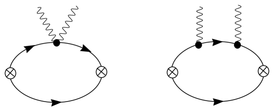
FIG. 1.: Leading order contributions to $\gamma$-deuteron Compton scattering. The crossed circles denote operators that create or annihilate two nucleons with the quantum numbers of the deuteron. The dark solid circles correspond to the photon coupling via the nucleon kinetic energy operator (minimal coupling). The solid lines are nucleons. The photon crossed graphs are not shown.

The types of graphs that will contribute to the $\gamma$-deuteron Compton scattering at LO (starting at $Q^{0}$) and NLO (starting at $Q^{1}$) can be classified as follows: minimal electric coupling, $C_{2}$, potential pion, magnetic moment coupling, nucleon electric polarizability, and nucleon magnetic polarizability. Power counting tells us at what order each of these begins to contribute. From eq. (14), pion loops contribute to the nucleon electric polarizability and scale as $1/m_{\pi}$ [35, 36, 37, 38, 39, 40, 41] at leading order, contributing to $\gamma$-deuteron Compton scattering at order $Q^{1}$. The nucleon magnetic polarizability also receives a contribution that behaves as $1/m_{\pi}$ in the chiral limit but is suppressed by a small numerical coefficient. It is thought that the nucleon magnetic polarizability will be dominated by $\Delta$ intermediate states. This type of pole graph scales like $m_{\pi}^{0}$ in the chiral limit[41], and therefore the magnetic polarizabilities contribute at order $Q^{2}$. The dimension-7 local polarizability counterterms in eq. (14) scale as $Q^{2}$. The nucleon electric polarizability contributes to $\gamma$-deuteron Compton scattering at NLO in regime II, but is suppressed by two additional powers of $Q$ in regime I. The $C_{2}$ operator in eq. (19) contributes at NLO.

The form factors $F$ and $G$ can be expanded in powers of $Q$,

$$\begin{array}[]{c}F=F^{LO}+F^{NLO}+...\quad,\\ G=G^{LO}+G^{NLO}+...\ \ \ ,\end{array}$$ (23)

It is convenient to introduce related form factors $\widetilde{F}$ and $\widetilde{G}$ which are related to $F$ and $G$ by

$$F(\omega,{\bf\hat{k}}\cdot{\bf\hat{k}^{{}^{\prime}}})\ = \ \widetilde{F}(\omega,{\bf\hat{k}}\cdot{\bf\hat{k}^{{}^{\prime}}})\ +\widetilde{F}(-\omega,{\bf\hat{k}}\cdot{\bf\hat{k}^{{}^{\prime}}})$$ (24)

$$G(\omega,{\bf\hat{k}}\cdot{\bf\hat{k}^{{}^{\prime}}})\ = \ \widetilde{G}(\omega,{\bf\hat{k}}\cdot{\bf\hat{k}^{{}^{\prime}}})\ +\ \widetilde{G}(-\omega,{\bf\hat{k}}\cdot{\bf\hat{k}^{{}^{\prime}}})\ \ \ ,$$ (25)

which also have expansions in powers of $Q$.

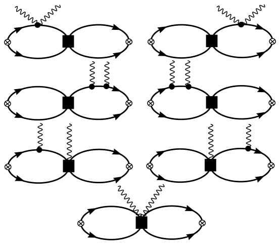
FIG. 2.: Graphs from insertions of the operator with coefficient $C_{2}(\mu)$ that contribute to $\gamma$-deuteron Compton scattering at NLO. The crossed circles denote operators that create or annihilate two nucleons with the quantum numbers of the deuteron. The solid circles correspond to the photon coupling via the nucleon kinetic energy operator (minimal coupling) while the solid square denotes the $C_{2}(\mu)$ operator. The solid lines are nucleons. Photon cross graphs are not shown.

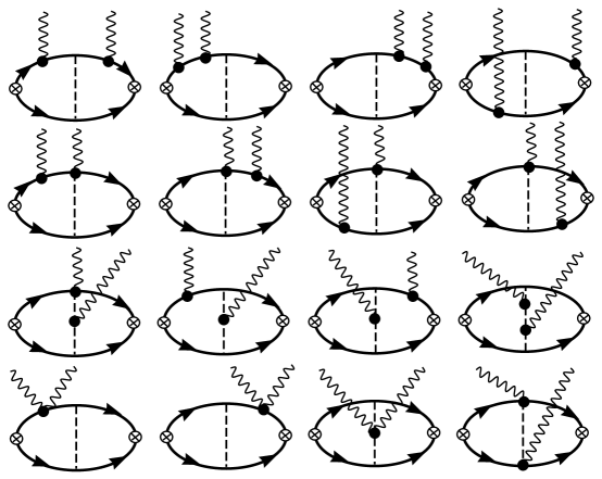
FIG. 3.: Graphs from the exchange of a single potential pion that contribute to $\gamma$-deuteron Compton scattering at NLO. The crossed circles denote operators that create or annihilate two nucleons with the quantum numbers of the deuteron. The solid circles correspond to the photon coupling via the nucleon or meson kinetic energy operator (minimal coupling) or from the gauged axial coupling to the meson field. Dashed lines are mesons and solid lines are nucleons. Photon crossed graphs are not shown.

A Regime I

In regime I (denoted by a subscript on the form factors), the LO contributions come from the electric coupling in the $N^{\dagger}{\bf D}^{2}N$ operator (minimal coupling), as shown in Fig. 1,

$$\widetilde{F}_{I}^{LO}\ =\widetilde{F}_{E}\quad,$$ (26)

with

$$\tilde{F}_{E} = -\left[{\sqrt{2}\gamma\over|\omega|\sqrt{1-{\bf\hat{k}}\cdot{\bf\hat{k}^{{}^{\prime}}}}}\tan^{-1}\left({|\omega|\sqrt{1-{\bf\hat{k}}\cdot{\bf\hat{k}^{{}^{\prime}}}}\over 2\sqrt{2}\gamma}\right)\ +\ {2\gamma^{4}\over 3M_{N}^{2}\omega^{2}}\ -\ {2\over 3}{\gamma(\gamma^{2}-M_{N}\omega-i\epsilon)^{3/2}\over M_{N}^{2}\omega^{2}}\right]\ \ \ .$$ (27)

In the form factors in eq. (27) we have neglected terms suppressed by additional factors of order ${\bf k}^{2}/M_{N}\omega$ (i.e. recoil effects) compared to the terms presented (the omitted recoil effects are NNLO in regime II). This approximation leads to a few percent correction to the rate. The maximum deviation of the arctangent term in eq. (27) from ${1\over 2}$ is approximately $\sim 15\%$ for $\omega=100\ {\rm MeV}$, the same magnitude as formally higher order terms in the $Q$ expansion.

The diagrams shown in Figs. 2 and 3 from insertions of the $C_{2}$ operator and the exchange of a single potential pion contribute at NLO in regime I. We write

$$\widetilde{F}_{I}^{NLO}=\widetilde{F}_{C_{2}}+\widetilde{F}_{\pi}\quad,$$ (28)

with the operator with coefficient $C_{2}$ contributing

$$\tilde{F}_{C2}=-{C_{2}(\mu)(\mu-\gamma)^{2}\gamma\over 3\pi M_{N}\omega^{2}} \left[\gamma^{4}-\gamma(\gamma^{2}-M_{N}\omega-i\epsilon)^{3/2}\right.$$ (30)

$$\left.+{3\over 4}M_{N}^{2}\omega^{2}\left(1-{\sqrt{2}\gamma\over|\omega|\sqrt{1-{\bf\hat{k}}\cdot{\bf\hat{k}^{{}^{\prime}}}}}\tan^{-1}\left({|\omega|\sqrt{1-{\bf\hat{k}}\cdot{\bf\hat{k}^{{}^{\prime}}}}\over 2\sqrt{2}\gamma}\right)\right)\right]\ \ \ .$$

The exchange of a single potential pion gives a contribution independent of the renormalization scale $\mu$, of

$$\tilde{F}_{\pi} = {g_{A}^{2}m_{\pi}\gamma\over 72\pi f^{2}\omega^{2}}\left[{m_{\pi}(m_{\pi}^{2}-2\gamma^{2}+2M_{N}\omega)\over M_{N}}\log\left[{m_{\pi}+2\sqrt{\gamma^{2}-M_{N}\omega-i\epsilon}\over\mu}\right]\right.$$ (36)

$$\left.\ -\ {2m_{\pi}(m_{\pi}^{2}-8\gamma^{2}+11M_{N}\omega)\over M_{N}}\log\left[{m_{\pi}+\gamma+\sqrt{\gamma^{2}-M_{N}\omega-i\epsilon}\over\mu}\right]\right.$$

$$\left.\ +\ {m_{\pi}(m_{\pi}^{2}-14\gamma^{2})\over M_{N}}\log\left[{m_{\pi}+2\gamma\over\mu}\right]\right.$$

$$\left.\ +\ {4\omega(M_{N}\omega-m_{\pi}^{2})\over m_{\pi}+\gamma+\sqrt{\gamma^{2}-M_{N}\omega-i\epsilon}}\ -\ {2M_{N}m_{\pi}\omega^{2}\over(m_{\pi}+2\gamma)^{2}}\right.$$

$$\left.\ +\ {4m_{\pi}\left(3(\gamma^{2}-M_{N}\omega)(\gamma-\sqrt{\gamma^{2}-M_{N}\omega-i\epsilon})\right)\over M_{N}(m_{\pi}+2\gamma)}\right.$$

$$\left.\ -\ {2\left(\gamma-\sqrt{\gamma^{2}-M_{N}\omega-i\epsilon}\right)(2M_{N}\omega-m_{\pi}\gamma)\over M_{N}}\right]\ \ \ .$$

In eq. (36) we have neglected the finite three-momentum transfer to the deuteron since it makes a numerically small modification to the amplitude. Therefore, we have not presented the complete calculation at NLO, but the omitted terms are numerically of order NNLO.

In regime I, the magnetic amplitudes vanish,

$$\widetilde{G}_{I}^{LO}=0\quad,\\ \widetilde{G}_{I}^{NLO}\ =0\quad,$$ (37)

and in the limit of $\omega\ll B,$ the full amplitude can be expanded in powers of $\omega/B$. The leading term is the Thomson limit for scattering from a charged deuteron

$${\cal M}=-i{\textstyle{\displaystyle e^{2}\over\displaystyle 2M_{N}}}\ {\bf\varepsilon\cdot\varepsilon}^{{}^{\prime}*}\ {\bf\varepsilon_{d}\cdot\varepsilon_{d}}^{{}^{\prime}*}\approx-i{\textstyle{\displaystyle e^{2}\over\displaystyle M_{d}}}{\bf\varepsilon\cdot\varepsilon}^{{}^{\prime}*}\ {\bf\varepsilon_{d}\cdot\varepsilon_{d}}^{{}^{\prime}*}\quad,$$ (38)

while the ($\omega/B)^{2}$ term gives the electric polarizability[33]. Another interesting limit is $B\rightarrow 0$ in which the forward scattering amplitude reduces to the Thomson limit for scattering from a charged proton, $-ie^{2}/M_{N}$.

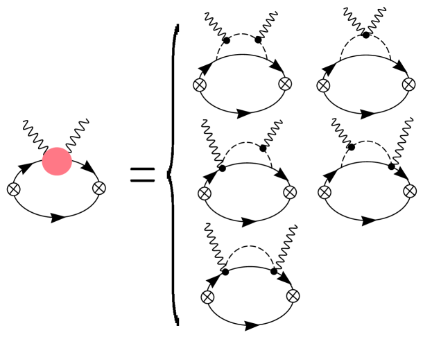
FIG. 4.: Pion graphs that contribute to the nucleon polarizabilities and to $\gamma$-deuteron Compton scattering at NLO. The crossed circles denote operators that create or annihilate two nucleons with the quantum numbers of the deuteron. The dark solid circles correspond to the photon coupling via the nucleon or pion kinetic energy operator or via the gauged axial pion-nucleon interaction. The solid lines are nucleons and the dashed lines are mesons. The photon crossed graphs are not shown.

In regime I, the nucleon polarizability diagrams (Fig. 4) and magnetic moment diagrams (Fig. 5) contribute at NNLO and N³LO, respectively. Therefore, in this regime the graphs that give rise to the nucleon polarizabilities make only a very small contribution to the polarizabilities of the deuteron. A more detailed discussion of this point can be found in ref. [33].

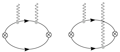
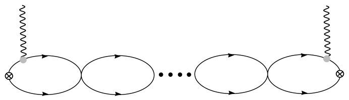
FIG. 5.: Graphs from insertions of the nucleon magnetic moment interaction that contribute to $\gamma$-deuteron Compton scattering at NLO. The crossed circles denote operators that create or annihilate two nucleons with the quantum numbers of the deuteron. The light solid circles denote the nucleon magnetic moment operator. The solid lines are nucleons. The bubble chain arises from insertions of the four nucleon operator with coefficient $C_{0}^{({}^{1}\kern-0.98ptS_{0})}$ or $C_{0}^{({}^{3}\kern-0.98ptS_{1})}$ .

B Regime II

In region II, the seagull diagram shown in Fig. 1 is LO while the other diagram in Fig. 1 (and the crossed graph) is demoted to higher order. At NLO, there are $C_{2}$ (Fig. 2) and single potential pion exchange (Fig. 3) diagrams, as in regime I. The new contributions at NLO are from insertions of the nucleon magnetic moment interactions (Fig. 5) and nucleon electric polarizability (Fig. 4) diagrams (the magnetic polarizability is negligible at this order because of the small numerical coefficient in the pion loop contribution and the counting of the $\Delta$ intermediate state) giving

$$\widetilde{F}_{II}^{LO} =\widetilde{F}_{E}\,\,,$$ (39)

$$\widetilde{F}_{II}^{NLO} =\widetilde{F}_{C_{2}}+\widetilde{F}_{\pi}+\widetilde{F}_{Npol}\,\,,$$ (40)

$$\widetilde{G}_{II}^{NO} =0\,\,,$$ (41)

$$\widetilde{G}_{II}^{NLO} =\widetilde{G}_{mag}\ \ \ \ ,$$ (42)

where $\widetilde{F}_{E},$ $\widetilde{F}_{C_{2}}$ and $\widetilde{F}_{\pi}$ are given in eqs. (27) (30) & (36).

The $C_{2}$ graphs present an interesting issue for power counting in regime II. In treating $M_{N}\omega$ of order $Q$, we find that individual $C_{2}$ graphs contribute at $Q^{1/2}$, $Q^{1}$, and $Q^{3/2}$. However, renormalization group invariance for the $C_{2}$ operator forces the sum of the graphs in the $C_{2}$ set to contribute at order $Q^{1}$ and higher.

The nucleon electric polarizability contribution at this order comes from the graphs shown in Fig. 4:

$$\widetilde{F}_{Npol} = {5g_{A}^{2}M_{N}\omega^{2}\over 48\pi f^{2}m_{\pi}}\ \left[{2\sqrt{2}\gamma\over|\omega|\sqrt{1-{\bf\hat{k}}\cdot{\bf\hat{k}^{{}^{\prime}}}}}\tan^{-1}\left({|\omega|\sqrt{1-{\bf\hat{k}}\cdot{\bf\hat{k}^{{}^{\prime}}}}\over 2\sqrt{2}\gamma}\right)\right]\left[1-{7\over 25}{\omega^{2}(1-{\bf\hat{k}}\cdot{\bf\hat{k}^{{}^{\prime}}})\over m_{\pi}^{2}}\right]\ \ \ ,$$ (43)

where an explicit factor of $e^{2}\over M_{N}$ has been removed to give the correct normalization for eq.(22). The momentum dependence in the “polarizability” contribution is generated both from the large size of the deuteron and from the fact that the pion mass sets the scale of the momentum dependence of electromagnetic properties of the nucleon. The leading momentum dependence of the pion contribution to the nucleon polarizability shown in eq. (43) has been computed in ref. [43]. Formally, all the momentum dependence is the same order in the $Q$ counting, as $Q\sim m_{\pi}\sim\omega$. The set of pion graphs shown in Fig. 4 gives an isoscalar nucleon electric polarizability[35] of

$$\alpha_{E,N} = {5g_{A}^{2}e^{2}\over 192\pi^{2}f^{2}m_{\pi}}\ =\ 1.2\times 10^{-3}\ {\rm fm}^{3}\ \ \ \ .$$ (44)

The magnetic moment contributions, Fig. (5), are

$$\widetilde{G}_{mag} ={\textstyle{\displaystyle 2(2\kappa^{(0)^{2}}+\kappa^{(1)^{2}})\gamma(\gamma-\sqrt{\gamma^{2}-M_{N}\omega-i\epsilon})\over\displaystyle 3M_{N}^{2}}}$$ (47)

$$+\ {\textstyle{\displaystyle\ \kappa^{(1)^{2}}\gamma(\gamma-\sqrt{\gamma^{2}-M_{N}\omega-i\epsilon})^{2}{\cal A}_{-1}^{(^{1}S_{0})}(\omega-B)\over\displaystyle 6\pi M_{N}}}$$

$$+{\textstyle{\displaystyle\ \kappa^{(0)^{2}}\gamma(\gamma-\sqrt{\gamma^{2}-M_{N}\omega-i\epsilon})^{2}{\cal A}_{-1}^{(^{3}S_{1})}(\omega-B)\over\displaystyle 3\pi M_{N}}}\quad,$$

where the leading order nucleon-nucleon scattering amplitude is[29, 30]

$${\cal A}_{-1}^{(^{1}S_{0}),(^{3}S_{1})}(E)\ =\ {\textstyle{-\displaystyle C_{0}^{(^{1}S_{0}),(^{3}S_{1})}\over\displaystyle{1}+\displaystyle C_{0}^{(^{1}S_{0}),(^{3}S_{1})}{\textstyle{\displaystyle M_{N}\over\displaystyle 4\pi}}(\mu-\sqrt{-M_{N}E-i\varepsilon}\ )}}\ \ \ \ .$$ (48)

The coefficient $C_{0}^{({}^{1}\kern-0.98ptS_{0})}$ has been determined from nucleon-nucleon scattering in the ${}^{1}\kern-1.4ptS_{0}$ channel [29] to be $C_{0}^{({}^{1}\kern-0.98ptS_{0})}=-3.34\ {\rm fm^{2}}$ while the coefficient $C_{0}^{(^{3}S_{1})}$ is given in eq. (21).

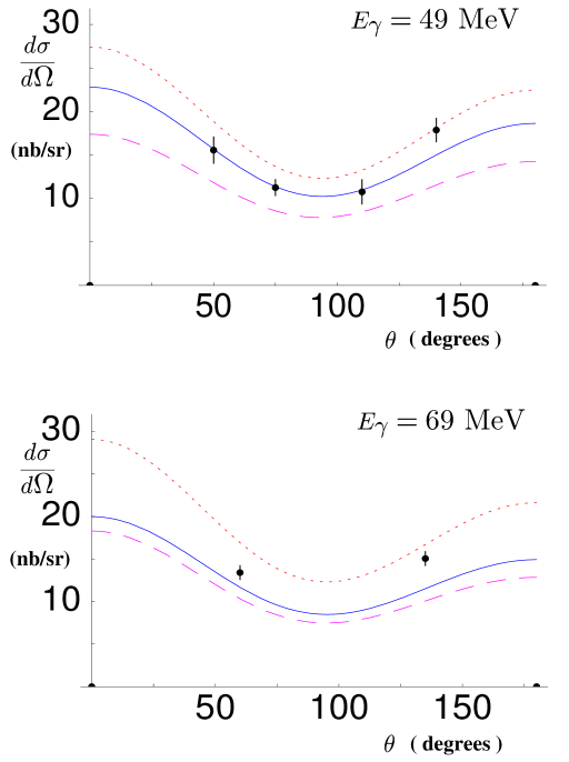
FIG. 6.: The differential cross section for $\gamma$-deuteron Compton scattering at incident photon energies of $E_{\gamma}=49\ {\rm MeV}$ and $69\ {\rm MeV}$. The dashed curves correspond to the LO result. The dotted curves correspond to the NLO result without the graphs that contribute to the polarizability of the nucleon. The solid curves correspond to the complete NLO result with no free parameters, as described in the text. Systematic and statistical errors associated with each data point have been added in quadrature.

The differential cross section written in terms of the electric and magnetic form factors in the deuteron rest frame is

$${\textstyle{\displaystyle d\sigma\over\displaystyle d\Omega}}_{lab}\ =\ {\textstyle{\displaystyle\alpha^{2}\over\displaystyle 2M_{N}^{2}}}\left[\ \left(\left|F_{II}(\omega)\right|^{2}\ +\ \left|G_{II}(\omega)\right|^{2}\right)\left(1\ +\ \cos^{2}\theta\right)\ +\ 4Re[F_{II}(\omega)G_{II}(\omega)^{*}]\cos\theta\ \right]\ \ \ \ ,$$ (49)

where $\cos\theta={\bf\hat{k}}\cdot{\bf\hat{k}^{{}^{\prime}}}$, the cosine of the angle between the incident and outgoing photons. Fig. 6 shows the differential cross section at photon energies of $49\ {\rm MeV}$ and $69\ {\rm MeV}$. The dashed curve on both plots is the LO prediction and is seen to underestimate the observed cross section. The dotted curve is the differential cross section at NLO but with the omission of the graphs (shown in Fig. 4) that contribute to the nucleon electric polarizability. The solid curve is the parameter free NLO prediction. We find excellent agreement with the data at $49\ {\rm MeV}$ and reasonable agreement with the data at $69\ {\rm MeV}$. It is clear from Fig. 6 that omission of the pion graphs that dominate the nucleon electric polarizability leads to an over-estimate of the differential cross section, as found in potential models [8, 9]. Further, the agreement between the data and the NLO calculation is comparable to the agreement between the data and potential model calculations [8, 9]. We estimate the size of the NNLO contributions to our calculation of the cross section to be about $10\%$, comparable to the experimental error associated with each data point. The analysis of [9] agrees well for the $69\ {\rm MeV}$ data and less well for the $49\ {\rm MeV}$ data while the analysis of [8] agrees reasonably well at both energies. When the effective field theory calculation is carried out to NNLO the prediction should be accurate to within $3\%$.

If we assume that the nucleon magnetic polarizability is the largest NNLO contribution and fit it to data we find a central value of

$$\beta_{M,N} = {1\over 2}(\beta_{M,p}+\beta_{M,n})\ =\ 6.5\times 10^{-4}\ {\rm fm}^{3}\ \ \ ,$$ (50)

but with a large uncertainty. The resulting differential cross section is shown in Fig. 7. Agreement with the data is improved but it must be stressed that there are many contributions at NNLO that need to be included before reliable conclusions can be drawn. Naive estimates of $\beta_{M,N}$ from $\Delta$ intermediate state pole-graphs suggest $\beta_{M,N}$ could be about $5\times 10^{-4}\ {\rm fm}^{3}$[41, 44].

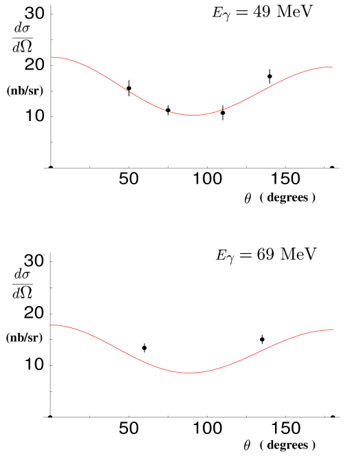
FIG. 7.: The differential cross section for $\gamma$-deuteron Compton scattering at incident photon energies of $E_{\gamma}=49\ {\rm MeV}$ and $69\ {\rm MeV}$. The curves correspond to the cross sections at NLO with the nucleon magnetic polarizability fit to the data. Systematic and statistical errors associated with each data point have been added in quadrature.

IV Conclusions

We have presented analytic expressions for the $\gamma$-deuteron Compton scattering amplitude at NLO in an effective field theory expansion. The parameter-free prediction for the differential cross section at NLO agrees very well at an incident photon energy of $49\ {\rm MeV}$ and reasonably well at $69\ {\rm MeV}$, as can be seen in Fig. 6. We see that pion graphs that dominate the electric polarizability of the nucleon are necessary to improve agreement with the measured $\gamma$-deuteron cross section.

The theoretical uncertainty in this calculation comes from the omission of terms at NNLO and higher in the effective field theory expansion, including the exchange of two potential pions, the exchange of a single radiation pion, insertions of the $C_{4}$ operator, relativistic effects, and the vector and tensor operators. These higher order terms could modify the differential cross section at the $10\%$ level. Calculation of the NNLO terms is required to be sure that the theory is reproducing the data at the few percent level.

We would like to thank David Kaplan, John Karakowski and Jerry Miller for helpful discussions. RPS thanks the nuclear theory group at the University of Washington for their hospitality. This work is supported in part by the U.S. Dept. of Energy under grants No. DE-FG03-97ER4014 and DE-FG02-96ER40945, and NSF grant number 9870475.

REFERENCES

[1] M. A. Lucas, Ph. D. thesis, University of Illinois at
Urbana-Champaign (1994)
[2] D. Drechsel et al, Summary of the working group on
Hadron Polarizabilities and Form Factors, nucl-th/9712013.
[3] E.L. Hallin et al, Phys. Rev. C 48, 1497 (1993).
[4] B.E. MacGibbon et al, Phys. Rev. C 52, 2097 (1995).
[5] J. Schmiedmayer et al, Phys. Rev. Lett.66, 1015 (1991).
[6] L. Koester et al, Phys. Rev. C 51, 3363 (1995).
[7] K. W. Rose et al., Phys. Lett. B 514, 621 (1990).
[8] M.I. Levchuk and A.I. L’vov, Few Body Systems Suppl.9, 439 (1995).
[9] T. Wilbois, P. Wilhelm and H. Arenhovel,
Few Body Systems Suppl.9, 263 (1995).
[10] J. Karakowski and G. Miller, private communication.
[11] S. Weinberg, Phys. Lett. B 251, 288 (1990);
Nucl. Phys. B 363, 3 (1991); Phys. Lett. B 295, 114 (1992).
[12] C. Ordonez and U. van Kolck, Phys. Lett. B 291, 459 (1992);
C. Ordonez, L. Ray and U. van Kolck, Phys. Rev. Lett.72, 1982 (1994) ;
Phys. Rev. C 53, 2086 (1996) ; U. van Kolck, Phys. Rev. C 49, 2932 (1994).
[13] T.S. Park, D.P. Min and M. Rho,
Phys. Rev. Lett.74, 4153 (1995) ; Nucl. Phys. A 596, 515 (1996).
[14] D.B. Kaplan, M.J. Savage and M.B. Wise,
Nucl. Phys. B 478, 629 (1996).
[15] T. Cohen, J.L. Friar, G.A. Miller and U. van Kolck,
Phys. Rev. C 53, 2661 (1996).
[16] D. B. Kaplan, Nucl. Phys. B 494, 471 (1997).
[17] T.D. Cohen, Phys. Rev. C 55, 67 (1997). D.R. Phillips
and T.D. Cohen, Phys. Lett. B 390, 7 (1997). K.A. Scaldeferri, D.R.
Phillips, C.W. Kao and T.D. Cohen, Phys. Rev. C 56, 679 (1997). S.R.
Beane, T.D. Cohen and D.R. Phillips, Nucl. Phys. A 632, 445 (1998).
[18] J.L. Friar, Few Body Syst. 99, 1 (1996).
[19] M.J. Savage, Phys. Rev. C 55, 2185 (1997).
[20] M. Luke and A.V. Manohar, Phys. Rev. D 55, 4129 (1997).
[21] G.P. Lepage, nucl-th/9706029, Lectures given at 9th
Jorge Andre Swieca Summer School: Particles and Fields, Sao Paulo, Brazil,
16-28 Feb 1997.
[22] S.K. Adhikari and A. Ghosh, J. Phys. A30, 6553 (1997).
[23] K.G. Richardson, M.C. Birse and J.A. McGovern,
hep-ph/9708435.
[24] P.F. Bedaque and U. van Kolck,
Phys. Lett. B 428, 221 (1998);
P.F. Bedaque, H.-W. Hammer and U. van Kolck,
Phys. Rev. C 58, R641 (1998).
[25] U. van Kolck, Talk given at Workshop on Chiral Dynamics:
Theory and Experiment (ChPT 97), Mainz, Germany, 1-5 Sep 1997.
hep-ph/9711222
[26] T.S. Park, K. Kubodera, D.P. Min and M. Rho,
Phys. Rev. C 58, R637 (1998); nucl-th/9807054.
[27] J. Gegelia, nucl-th/9802038;
nucl-th/9806028.
[28] J.V. Steele and R.J. Furnstahl,
Nucl. Phys. A 637, 46 (1998); nucl-th/9808022.
[29] D.B. Kaplan, M.J. Savage and M.B. Wise,
Phys. Lett. B 424, 390 (1998);
nucl-th/9802075, to appear in Nucl. Phys. B;
[30] D.B. Kaplan, M.J. Savage, and M.B. Wise,
nucl-th/9804032.
[31] M.J. Savage,
Including Pions, talk presented at the
Workshop on Nuclear Physics with Effective Field Theories,
Caltech (1998), nucl-th/9804034;
What Effective Field Theory May Contribute to the BLAST Program,
talk presented at the
2nd Workshop on Electronuclear Physics with Internal Targets
and the BLAST Detector, MIT (1998), nucl-th/9807023.
[32] T. Cohen and J.M. Hansen,
nucl-th/9808006; nucl-th/9808038.
[33] J. W. Chen, H. W. Grießhammer, M.J. Savage, and R. P.
Springer, nucl-th/9806080.
[34] M.J. Savage and R.P. Springer, nucl-th/9807014.
D.B. Kaplan, M.J. Savage, R.P. Springer and M.B. Wise,
nucl-th/9807081.
[35] V. Bernard, N. Kaiser and U. Meissner,
Phys. Rev. Lett.67, 1515 (1991);
Nucl. Phys. B 373, 364 (1992);
Phys. Lett. B 319, 269 (1993).
[36] V. Bernard, N. Kaiser J. Kambor and U. Meissner,
Nucl. Phys. B 388, 315 (1992);
[37] M.N. Butler and M.J. Savage, Phys. Lett. B 294, 369 (1992).
[38] A.I. L’vov, Int. J. Mod. Phys. A 8, 5267 (1993).
[39] B.R. Holstein and A.M. Nathan,
Phys. Rev. D 49, 6101 (1994).
[40] B.R. Holstein, hep-ph/9710548.
[41] M.N. Butler, M.J. Savage and R.P Springer,
Nucl. Phys. B 399, 69 (1993).
[42] P.A.M. Guichion, G.Q. Liu and A.W. Thomas,
Nucl. Phys. A 591, 606 (1995).
[43] T.R. Hemmert, B.R. Holstein, G. Knochlein and S. Scherer,
Nucl. Phys. A 631, 607c (1998).