Nuclear Transport at Small Excitations: Thermal and Quantal Aspects

Abstract

The application of the locally harmonic approximation to large scale collective motion is briefly reviewed. Particular emphasis is paid to issues which might be useful in the more general context, or which are specific to our treatment, like there are: Self-consistency between collective and intrinsic motion, a $T$ dependent coupling constant, the inclusion of quantum effects for the dynamics of fluctuations. Finally, open problems are addressed, like the use of thermodynamic concepts at smaller excitations, the ergodicity question, the variation of transport coefficients with the nuclear shape due to shell structure, the limits of the LHA at smaller $T$.

1 Introduction

In this talk I would like to briefly report on the transport theory which has been worked out on the basis of a suitable application of linear response theory. In the second part I shall address some of the most stringent and largely unresolved problems one generally faces in dealing with nuclear transport at smaller excitations. Details will be presented only to outline the general concepts. For more extensive studies I like to refer to my recent review article [1] as well as to the original papers, especially to those of the more recent years which have been published together with F.A. Ivanyuk, D. Kiderlen and S. Yamaji and others.

1.1 The basic approximation scheme

Unfortunately, still too often theories of nuclear collective motion are considered separately from transport models. This is unjust both in the light of present day experiments as well as from the more general point of view. Indeed, it is probably only for rotational motion exactly along the Yrast line that intrinsic excitations of the nuclear system do not play any role. Moreover, one should not forget that one of the first theoretical descriptions of the prime example of large scale collective motion, nuclear fission, was given by Kramers [2] as early as 1940 and which was based on the picture of ”transport” in collective phase space. In his famous equation there appear such concepts as dissipation and stochasticity. (The reader who is not familiar with this equation is asked to wait for a short while; we will come back to it later). Kramers applied this equation to the decay rate for fission, to find a generalization of the famous Bohr-Wheeler formula. In these days the origin of dissipation was attributed to the strong ”correlations” among the nucleons, as they can be understood within or follow from N. Bohr’s compound nucleus. Below we shall try to elaborate on such a point of view on the basis of our present day understanding of nuclear dynamics. First we want to explain why and in which way large scale motion may be described by a linear response approach.

The basic element is the observation that motion in the collective phase space may be expressed in terms of propagators by writing for the time evolution of the density distribution

$$f(Q,P,t)=\int{\rm d}Q_{0}{\rm d}P_{0}\;\;K(Q,P,t;Q_{0},P_{0},t_{0})\;\;f(Q_{0},P_{0},t_{0})$$ (1)

with $\lim_{t\to t_{0}}{K(Q,P,t;Q_{0},P_{0},t_{0})}=\delta(Q-Q(t_{0}))\delta(P-P(t_{0}))$

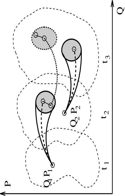
Figure 1: Time development of global motion within the propagator method. For the time step from $t_{2}$ to $t_{3}$ the related Langevin method is indicated.

Here $K(Q,P,t;Q_{0},P_{0},t_{0})$ may be interpreted as the conditional probability for the system to move from $Q_{0},P_{0}$ at $t_{0}$ to $Q,P$ at time $t$. On both sides of this relation the distribution $f$, the ”joint probability”, may be replaced by conditional probabilities defining the transition say from a $t_{0}$ to the final time $t$ through an intermediate step at $t_{1}$. The resulting relation is nothing else but the Chapman-Kolmogorov equation. (For a discussion of such general properties we may refer to the book by van Kampen [3]).

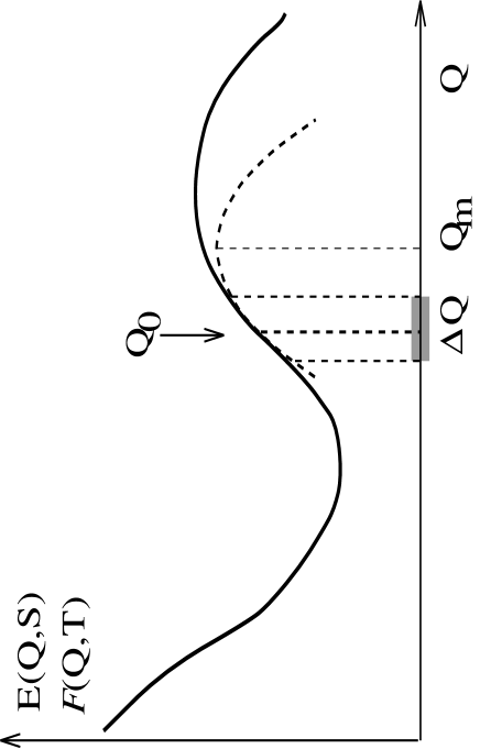
Figure 2: The LHA to a typical fission potential, which may either be given by the internal or the free energy.

The procedure just described may be repeated introducing small time steps $\delta t$. They only must be chosen longer than the typical microscopic time $\tau$ below which an averaging over the microscopic dynamics of the nucleons would become meaningless. A linear response approach becomes possible whenever the $\delta t$ is small on the collective time scale. Consequently, the $K(Q,P,t;Q_{0},P_{0},t_{0})$ may be constructed within a locally harmonic approximation (LHA), to collective motion. If this propagator spreads over a limited regime of phase space only, within the time lap $\delta t$, a Gaussian form will do. A pictorial view of this method is given in Figs.1 and 2.

1.2 The equation of motion for the propagator

To approximate the propagator by a Gaussian means to write:

$$K_{G}(Q,P,t;Q_{0},P_{0},t_{0})=(2\pi)^{-1}{\it\Delta}^{-1/2}\;\exp\Bigl{\{}-{1\over 2}\sum_{i,k}({\cal X}_{i}-{\cal X}_{i}^{c}(t))({\cal X}_{k}-{\cal X}_{k}^{c}(t)){\cal A}_{ik}(t)\Bigr{\}}$$ (2)

with the ${\it\Delta}(t)$ being the determinant ${\it\Delta}(t)=\det\bigl{(}{\cal A}^{-1}_{ik}(t)\bigr{)}$. The vector ${\cal X}$ defines a point in collective phase space, and the $K_{G}$ represents a distribution, centered at the trajectory ${{\cal X}^{c}(t)}$, which starts at $P_{0},Q_{0}$,

$${\cal X}=\pmatrix{P\cr Q\cr}\qquad{{\cal X}^{c}(t)}=\pmatrix{P^{c}(t)\cr Q^{c}(t)\cr}=\pmatrix{\big{\langle}P\big{\rangle}_{t}\cr\big{\langle}Q\big{\rangle}_{t}\cr}\qquad\pmatrix{P_{0}\cr Q_{0}\cr}=\pmatrix{P(t_{0})\cr Q(t_{0})\cr}$$ (3)

and which fulfills the following set of equations:

$$P^{c}(t)=M{dq^{c}\over dt}\qquad\qquad{dP\over dt}=-Cq^{c}(t)-\gamma{dq^{c}\over dt}$$ (4)

Here we have introduced the variable $q=Q-Q_{m}$. The $Q_{m}$ defines the position of the local oscillator, more precisely the position of the extremum of the local, effective collective potential. It is a linear function of $Q(t_{0})$, and has to be defined by the condition that the constant term in the force disappears see Fig.2 and below.

The matrix ${\cal A}_{ik}(t)$ is given by the widths of the distribution

$$\bigl{(}{\cal A}(t)\bigr{)}^{-1}=\pmatrix{{\textstyle\sum}_{pp}\!(t)&{\textstyle\sum}_{qp}\!(t)\cr{\textstyle\sum}_{qp}\!(t)&{\textstyle\sum}_{qq}\!(t)\cr}$$ (5)

with the ${\textstyle\sum}_{qq}\!(t)$ etc. being defined as ${\textstyle\sum}_{qq}\!(t)=\big{\langle}(Q-Q^{c}(t))^{2}\big{\rangle}_{t}\equiv\big{\langle}Q^{2}\big{\rangle}_{t}-(Q^{c}(t))^{2}$. These second moments fulfill the following set of equations:

$${d\over dt}{\textstyle\sum}_{qq}\!(t)-{2\over M}{\textstyle\sum}_{qp}\!(t)=0$$ (6)

$${d\over dt}{\textstyle\sum}_{qp}\!(t)-{1\over M}{\textstyle\sum}_{pp}\!(t)+C{\textstyle\sum}_{qq}\!(t)+{\gamma\over M}{\textstyle\sum}_{qp}\!(t)=D_{qp}$$ (7)

$${d\over dt}{\textstyle\sum}_{pp}\!(t)+2C{\textstyle\sum}_{qp}\!(t)+2{\gamma\over M}{\textstyle\sum}_{pp}\!(t)=2D_{pp}$$ (8)

The inhomogeneities represent the diffusion coefficients. The initial condition ${\textstyle\sum}_{qq}\!(t_{0})={\textstyle\sum}_{qp}\!(t_{0})={\textstyle\sum}_{pp}\!(t_{0})=0$ warrants the $K_{G}$ to start from the sharp distribution as required by (1).

This $K_{G}$ satisfies the following transport equation

$${\partial\over\partial t}f(q,P,t)=\Biggl{[}-{\partial\over\partial q}{P\over M}+{\partial\over\partial P}Cq+{\partial\over\partial P}{P\over M}\gamma+D_{qp}{\partial^{2}\over\partial q\partial P}+D_{pp}{\partial^{2}\over\partial P\partial P}\Biggr{]}f(q,P,t)$$ (9)

This is easily verified by mere differentiation. The form of this equation resembles the one of Kramers with the exception that in his case the diffusion coefficients were given by $D_{pp}=\gamma T$ and $D_{qp}=0$. Moreover, as he understood his equation to describe large scale motion, the conservative force was given by the derivative of the full potential, $-\partial V(q)/\partial q$, rather than by $-Cq$.

2 The derivation of the EOM within the LHA

In this chapter we are going to describe briefly how we may obtain the transport coefficients as they appear in (9), or in the equations for the first (4) and second moments (6-8). To this end let us assume to be given a Q-dependent Hamiltonian of the type $\hat{H}(\hat{x}_{i},\hat{p}_{i},Q)=\hat{H}_{sp}(Q)+\hat{V}^{(2)}_{\rm res}({\hat{x}}_{i},{\hat{p}}_{i})$ The term $\hat{H}_{sp}(Q)$ represents independent particle motion in a deformed shell model, with Strutinsky renormalization meant to be included. The $\hat{V}^{(2)}_{\rm res}({\hat{x}}_{i},{\hat{p}}_{i})$ stands for a residual interactions, considered finally by way of a complex self-energies of the single particles: ${\it\Sigma}(\omega\pm i\epsilon,T)=\Sigma^{\prime}(\omega,T)\mp{i\over 2}\Gamma(\omega,T)$. Microscopic expressions are then calculated after replacing the single particle strength $\varrho_{k}(\omega)=2\pi\;\delta(\hbar\omega-e_{k})$ by

$$\varrho_{k}={\Gamma(\omega)\over\left(\hbar\omega-e_{k}-\Sigma^{\prime}(\omega)\right)^{2}+\left({\Gamma(\omega)\over 2}\right)^{2}}\qquad\Gamma={1\over\Gamma_{0}}\;{(\hbar\omega-\mu)^{2}+\pi^{2}T^{2}\over 1+\left[(\hbar\omega-\mu)^{2}+\pi^{2}T^{2}\right]/c^{2}}$$ (10)

with the $\mu$ being the chemical potential. The $\Gamma$ is understood to represent ”collisional damping”. In numerical computations, the following values have mostly been used for the parameters entering here: $\Gamma_{0}=33\;{\rm MeV}$ and $c=20\;{\rm MeV}$.

2.1 Average motion

2.1.1 Secular equation from energy conservation

An equation of average motion may be obtained from energy conservation [5], regarding the nucleus as an isolated system. One may thus write $0={d\over dt}E_{\rm tot}={\dot{Q}}\left<{\partial\hat{H}({\hat{x}}_{i},{\hat{p}}_{i},Q)\over\partial Q}\right>_{t}\equiv{\dot{Q}}\left<\hat{F}({\hat{x}}_{i},{\hat{p}}_{i},Q)\right>_{t}$, to get the equation of motion for $Q(t)$ after expressing the average $\left<\hat{F}({\hat{x}}_{i},{\hat{p}}_{i},Q)\right>_{t}$ as a functional of $Q(t)$. Following the scheme of the LHA one may expand the $\hat{H}(Q)$ around any given $Q_{0}$ to have:

$$\hat{H}(Q(t))=\hat{H}(Q_{0})+(Q(t)-Q_{0}){\hat{F}}+{1\over 2}(Q(t)-Q_{0})^{2}\left<{\partial^{2}\hat{H}\over\partial Q^{2}}(Q_{0})\right>^{\rm qs}_{Q_{0},T_{0}}$$ (11)

The effects of the coupling term $(Q(t)-Q_{0}){\hat{F}}$ may then be treated by linear response theory, exploiting as a powerful tool the causal response function ${\widetilde{\chi}}$

$${\widetilde{\chi}}(t-s)=\Theta(t-s){i\over\hbar}{\rm tr}\,\left(\hat{\rho}_{\rm qs}(Q_{0},T_{0})[\hat{F}^{I}(t),\hat{F}^{I}(s)]\right)\equiv 2i\Theta(t-s){\widetilde{\chi}}^{\prime\prime}(t-s)$$ (12)

Here, the time evolution in $\hat{F}^{I}(t)$ as well as the density operator $\hat{\rho}_{\rm qs}$ are determined by $H(Q_{0})$. The $\hat{\rho}_{\rm qs}$ is meant to represent thermal equilibrium at $Q_{0}$ with excitation being parameterized by temperature $T_{0}$ or by entropy $S_{0}$.

The equation of motion may finally be brought to the form $k^{-1}q(t)+\int_{-\infty}^{\infty}\widetilde{\chi}(t-s)q(s){\rm d}s=0$ whose Fourier transform leads to the well known form of the secular equation for the possible local frequencies of the harmonic motion: $k^{-1}+\chi(\omega)=0$. Its solution will be discussed below. The $q(t)$ is given by

$$q(t)=Q(t)-Q_{m}\qquad{\rm with}\qquad\left.{\partial E(Q,S_{0})\over\partial Q}\right|_{Q_{0}}+\left.{\partial^{2}E(Q,S_{0})\over\partial Q^{2}}\right|_{Q_{0}}(Q_{m}-Q_{0})=0$$ (13)

and $Q_{m}$ represents the position of the center of the local oscillator and the $k$ a coupling constant, which for the case of zero temperature is known from the Copenhagen version of describing harmonic vibrations [6]. At finite thermal excitations things become more complicated, where besides the shape variable itself also the parameter specifying the state of the system may change in time. Choosing entropy, however, one may argue this change to happen only in second order in the velocity. For harmonic motion this is beyond the order to be considered. Keeping $S$ constant one then obtains [4]

$$-k^{-1}=\left<{\partial^{2}\hat{H}\over\partial Q^{2}}(Q_{0})\right>^{\rm qs}_{Q_{0},T_{0}}+(\chi(0)-\chi^{\rm ad})=\left.{\partial^{2}E(Q,S_{0})\over\partial Q^{2}}\right|_{Q_{0}}+\chi(0)$$ (14)

The $\chi^{\rm ad}=-\left({\partial<\hat{F}>\over\partial Q_{0}}\right)_{S}$ is the adiabatic susceptibility and $E(Q,S_{0})$ is the internal energy. As the latter is somewhat difficult to evaluate one may introduce the free energy to rewrite (14) as

$$-k^{-1}=\left.{\partial^{2}{\cal F}(Q,T_{0})\over\partial Q^{2}}\right|_{Q_{0}}+\chi(0)-\left({1\over{\partial^{2}{\cal F}\over\partial T^{2}}}\left({\partial^{2}{\cal F}\over\partial T\partial Q}\right)^{2}\right)_{Q_{0},T_{0}}$$ (15)

Notice, please, that for constant entropy $S$ one may, for the quasi-static case, relate the temperature change to the one of the collective coordinate itself by applying general rules from thermodynamics: $dT=\left({\partial T/\partial Q}\right)_{S}dQ$.

Another point which we want to elaborate further below concerns the difference between the adiabatic susceptibility and the static response, which can be shown to be either positive or zero. It vanishes at zero thermal excitations but at finite temperature it does so only for ergodic systems, a problem to which we shall return below:

$$\chi^{\rm ad}-\chi(0)=0$$ (16)

2.1.2 The collective response

Let us introduce a coupling $q_{ext}F$ to a time dependent ”external field” $f_{\rm ext}(t)$ by adding $f_{\rm ext}(t)\hat{F}$ to our Hamiltonian: $\hat{H}^{\prime}=\hat{H}({\hat{x}}_{i},{\hat{p}}_{i},Q)+f_{\rm ext}(t)\hat{F}$ but where $\hat{H}(Q)$ is taken in the approximate form (11). The coupling is chosen to have the same form as the one between the two ”subsystems” of collective and nucleonic degrees of freedom, with only the $(Q(t)-Q_{0})$ replaced by the ”external field” $f_{\rm ext}$. The ”collective” response function may now be defined as:

$$\delta\langle\hat{F}\rangle_{\omega}=-\chi_{{\rm coll}}(\omega)f_{\rm ext}(\omega)$$ (17)

where for convenience we have switched to frequency representation. The difference between the $\delta\langle\hat{F}\rangle_{\omega}$ and the $\langle\hat{F}\rangle_{\omega}$ should at best have a term proportional to $\delta(\omega)$, representing some static force in the time dependent picture. The phrase ”collective” response function is chosen because i) this function now includes the collective excitations as well and ii) we will later on consider the latter as the only interesting ones.

The construction of the $\chi_{\rm coll}(\omega)$ can be done following the derivation of the polarizability function for electric media as introduced by Clausius and Mosotti, and as described in [6] for the nuclear case at zero excitation. We need three equations: Besides the basic definition (17), we have to have an equation which relates $\langle\hat{F}\rangle_{t}$ to $(Q(t)-Q_{0})$ and we need to express $\langle\hat{F}\rangle_{t}$ by the total perturbation consisting of both external and induced fields. We want to perform this construction assuming ergodicity for our nucleonic system, i.e. requiring the condition (16) to be fulfilled. Exploiting (14) the relation between the average $\langle\hat{F}\rangle_{t}$ and the deviation of $Q$ from $Q_{0}$ becomes

$$k\langle\hat{F}\rangle_{t}=Q-Q_{0}$$ (18)

Finally, the collective response function defined by (17) takes on the form

$$\chi_{{\rm coll}}(\omega)={\chi(\omega)\over 1+k\chi(\omega)}$$ (19)

The relation (18) reminds one of a self-consistency condition, like one would find treating an effective two-body interaction $(k/2){\hat{F}}{\hat{F}}$ in mean field approximation. However, such a notion is justified on more general grounds. It is this relation (18) which expresses most clearly that the correct interpretation of the $Q(t)$ must be to consider this quantity an internal variable—measuring some properties of the nucleus and clearly to be distinguished from truly external fields like the $f_{\rm ext}$.

2.1.3 Transport Coefficients and the distribution of collective strength

The procedure of defining the transport coefficient of inertia, friction and local stiffness is as follows: For selected peaks of the strength distribution one fits the dissipative part of the oscillator response $\chi_{\rm osc}(\omega)=\left(M\omega^{2}+i\gamma\omega-C\right)^{-1}$ to the $\chi_{{\rm coll}}(\omega)$ calculated microscopically. If one is interested in the transport coefficients for the $q-$motion one first transforms to the response function $\chi_{qq}(\omega)$ in the $q$-mode, defined through $\chi_{qq}(\omega)={\delta q(\omega)/\delta(-q_{\rm ext}(\omega)}\mid_{q_{\rm ext}=0}$. This can easily be done with the help of the linear relation: $k\delta\langle\hat{F}\rangle_{t}=\delta Q(t)\equiv q(t)$ which implies $\chi_{qq}(\omega)=k^{2}\chi_{{\rm coll}}(\omega)$. Summarizing, this fit then implies the substitution (with $\omega_{1}^{\pm}=\pm{\cal E}-i\Gamma/2$)

$$\chi_{qq}(\omega)\;\Longrightarrow\;\chi_{\rm osc}(\omega)={-1\over M(\omega_{1}^{+}-\omega_{1}^{-})}\left({1\over\omega-\omega_{1}^{+}}-{1\over\omega-\omega_{1}^{-}}\right)$$ (20)

in a certain range frequencies which encompasses the peak in the strength distribution whose associated mode $\omega_{1}$ one wants to treat explicitly. Notice, please, that in this way we actually solve the secular equation for arbitrary damping. In the case of fission it is believed that it is mainly the low frequency behavior which matters, for which reason it is the lowest peak which is treated in this way. For an application to giant resonances see [7] for the case of the quadrupole and the talk by S. Yamaji at this meeting for monopole vibrations.

Within the formulation presented above the strength distribution may change dramatically with temperature [7], [8], [9]. This is mainly due to the temperature dependence of the coupling constant, as determined by the stiffness $C(0)=\partial^{2}E(Q,S_{0})/\partial Q^{2}$ of the static energy (see (14)). For the quadrupole as well as for the local motion along the fission path, the $C(0)$ may well decrease by more than an order of magnitude when $T$ is increased from $0$ to about $2\cdots 3\;{\rm MeV}$. As a consequence, at the higher temperatures practically all strength concentrates in one dominant low frequency mode, with the associated transport coefficients reflecting strongly over-damped motion. This feature has been demonstrated in [7] (see Fig..1 of this reference or Fig.5.1.1 of [1]). As may be expected from such a strength distribution, the inertia of the low frequency mode decreases from the typical cranking model value at low excitations to the one given by the energy weighted sum rule at large $T$ [7].

Conveniently the transport coefficients are expressed by the following ratios

$${\Gamma}={\gamma\over M}\;\;\;\quad\;\;\;\;\;\;\quad\;\;\;\varpi^{2}={{\mid C\mid}\over M}\;\;\;\quad\;\;\;\;\;\;\quad\;\;\;\eta={\gamma\over 2\sqrt{M\mid C\mid}}$$ (21)

with which the frequencies the two frequencies may be expressed as $\omega^{\pm}=\pm{\cal E}-i{\Gamma\over 2}=\varpi\left(\pm\sqrt{{\rm sign}C-\eta^{2}}-i\eta\right)$. Numerical values from microscopic computations can be found in [8], [9] and [10]. A typical calculation of $\Gamma$ is shown in Fig.3 (from [10]). If evaluated at the potential minimum and at the barrier, typically the $\hbar\varpi$ is of the order of $1\;{\rm MeV}$, independently of $T$; conversely the $\eta$ increases from about $1$ at $T=1\;{\rm MeV}$ to about $3$ at $5\;{\rm MeV}$ [10].

Figure 3: The inverse relaxation time $\Gamma=\gamma(\omega_{1})/M(\omega_{1})$ as function of deformation and temperature (indicated in the Figure).

The behavior found in our model for the strength distribution may be understood in the sense of reaching a macroscopic limit with increasing $T$. Within such a limit there is no room any more neither for quantal coherence in the sense of collective motion nor for the typical single particle excitations. The nucleus just behaves like a drop of a strongly viscous nuclear fluid (see also [11], [12]). This behavior is in clear contrast to the one found for common RPA at finite $T$, for instance like in the so called ”thermo field theory” (see talks at this meeting and c.f. [13]).

2.1.4 The equation of average motion and the transfer of heat

After the substitution (20) the equation for the $q$-mode attains the form:

$$M(\omega{{}_{1}})\,{\ddot{q}}(t)+\gamma(\omega{{}_{1}})\,{\dot{q}}(t)+C(\omega{{}_{1}})\,q(t)=-q_{\rm ext}(t)$$ (22)

It is of differential nature although we have not really made use of any Markovian approximation. All we did is to restrict ourselves to just one mode assuming that the associated peak can be approximated by a Lorentzian. For these reasons we are actually dealing with Non-Markovian transport coefficients representing dynamics in a whole range of frequencies. They are determined uniquely for under- as well as for over-damped motion, and for positive or negative stiffness.

Let us turn to the energy balance once more. One finds the equation

$${d\over dt}E_{\rm tot}={d\over dt}\left({M{\dot{q}}^{2}\over 2}+{Cq^{2}\over 2}\right)+\gamma\dot{q}^{2}={d\over dt}E_{\rm coll}+T{dS\over dt}$$ (23)

no matter whether the external field is ”switched on or off” [4]. For (damped) self-sustained motion the equation ${dE_{\rm tot}/dt}=0$ may thus be rewritten as

$$-{d\over dt}E_{\rm coll}\equiv-{d\over dt}\left({M(\omega_{1})\over 2}{\dot{q}}^{2}+{C(\omega_{1})\over 2}q^{2}\right)=\gamma(\omega_{1}){\dot{q}}^{2}\equiv T{d\over dt}S$$ (24)

which correctly expresses the exchange between collective motion into heat.

2.2 The dynamics of fluctuations of the collective degrees of freedom

So far the collective variable $Q$ was just a c-number classifying the deformation of the mean field. To be able studying collective fluctuations we first must raise $Q$ to become a genuine dynamical variable. As we are interested in quantum effects this generalization has to be performed in operator sense. Simultaneously, we need to introduce the associated momentum $\hat{\Pi}$, and we must find a decent Hamiltonian for the total system. Such a Hamiltonian may then be used to derive the transport equation for the collective density operator $\hat{d}$, the Wigner function of which may be associated with the distribution in collective phase space mentioned before. Evidently, such a procedure ought to account for the basic and important features we have been able to consider for average motion, the most stringent one perhaps being self-consistency. If at all possible, this ambitious program can be accomplished only in a restrictive sense; here it will be the LHA approximation, once more, which is exploited.

2.2.1 A suitable Hamiltonian for the total system

We would like to have a Hamiltonian which splits into parts of nucleonic and collective motion plus a coupling between both subsystems: $\hat{\cal H}=\hat{H}_{\rm nucl}+\hat{H}_{\rm coup}+\hat{H}_{\rm coll}$. This goal may be achieved by applying the Bohm-Pines method, which originally has been invented to treat collective modes in the electron gas. One obtains:

$$\hat{\cal H}=\hat{H}(\hat{x}_{i},\hat{p}_{i},Q_{0})+k\hat{\Pi}\hat{\dot{F}}-{\beta\over k}(\hat{Q}-Q_{0})\hat{F}+{\hat{\Pi}^{2}\over 2m_{0}}+{1\over 2k^{2}}(2\beta+k)(\hat{Q}-Q_{0})^{2}$$ (25)

The unperturbed collective inertia is given by the sum rule value, namely

$${1\over m_{0}}=ik^{2}\;\langle\,[\hat{\dot{F}},\hat{F}]\,\rangle_{Q_{0}}\qquad\qquad\hat{\dot{F}}=i\;[\hat{H}(Q_{0}),\hat{F}]$$ (26)

The $\hat{\Pi}$ is the canonical momentum satisfying the commutation rule $[\hat{Q},\hat{\Pi}]=i\hbar$.

The intrinsic part obtains a most convenient form: It is the same $\hat{H}(\hat{x}_{i},\hat{p}_{i},Q_{0})$ which appeared already in (11) as the unperturbed part. The important point is that there is no reduction of the number of nucleonic degrees of freedom. This implies that we will be able to work with the same nucleonic response functions as before. Of course, in order not to have too many degrees of freedom there will have to be a subsidiary condition, which turns out to be

$$k\hat{F}-(\hat{Q}-Q_{0})=0$$ (27)

For average motion it reduces to the form (18) found before. Notice the two coupling terms: The first one is of similar structure as that in (11). In addition there is term involving $\hat{P}$, which is multiplied by the same factor $\hat{\dot{F}}$ which appears also in the unperturbed inertia. It is this intimate relation between the coupling terms and the unperturbed collective Hamiltonian which in the end assures self-consistency, in the sense of the collective coordinate being related to the intrinsic field $\hat{F}$. The alert reader will have noticed that there is the additional parameter $\beta$. In the end the latter is chosen as $(\beta+k)/k^{2}=C=-M\omega_{1}^{+}\omega_{1}^{-}$, Very naturally this goes along with the re-introduction of the kinetic momentum, such that for the averaged dynamics one regains the form (4).

For undamped motion the situation is like in common RPA: The Hamiltonian can be transformed in such a way that the coupling between collective and nucleonic degrees of freedom effectively shows up in renormalized transport coefficients for inertia and stiffness, after the intrinsic degrees of freedom have been averaged out. The corresponding frequency satisfies the secular equation of RPA which corresponds to the separable interaction $(k/2){\hat{F}}{\hat{F}}$. This equation has the form given above but where in the $\chi$ only the reactive part plays a role. For damped motion the situation is more complicated. To get information about the dynamics of collective fluctuations one needs to invoke projection techniques, like the one of the Nakajima-Zwanzig method.

2.2.2 A non-perturbative Nakajima-Zwanzig approach

One starts with the von Neumann equation for the Hamiltonian (25) and defines the reduced density $\hat{d}$ by averaging out the intrinsic degrees of freedom. Its equation has a term which is non-local in time. The integral kernel $\cal K$ contains an operator for the time evolution of the total system, which commonly is treated in second order perturbation theory, the argument being that $\cal K$ does already contain the coupling twice. However, in order to meet the standard set up at the beginning of this subsection one needs to do better. The new scheme to be applied may be read of from the structure of the collective response function (19): On the one hand one may exploit low order perturbation theory with respect to the effects of the coupling on the intrinsic degrees of freedom, for which reason the nucleonic response function $\chi$ appears. Conversely, with respect to collective motion an infinite order is considered, as seen by the fact that the coupling constant appears in the denominator. To translate this scheme to the NZ approach essentially one replaces the unperturbed time evolution operator by an effective one:

$$\exp[-i(\hat{L}_{\rm coll}+\hat{L}_{\rm nucl})s]\quad\Longrightarrow\quad\exp[-i(\hat{\cal L}^{eff}_{\rm coll}+\hat{L}_{\rm nucl})s]$$ (28)

Here, time evolution is formulated in terms of Liouvillians. Fortunately, the effective one, $\hat{\cal L}^{eff}_{\rm coll}$, need not be constructed explicitly if we are interested only in the Gaussian form of the local propagators introduced in sect.1. It suffices to exploit the quantal fluctuation dissipation theorem, which can be proven to be satisfied within the modified Nakajima-Zwanzig approach.

2.2.3 Diffusion coefficients and the equilibrium of the damped oscillator

Let us turn our attention to equilibrium fluctuations first. Imagine the total system to be close to equilibrium at some given temperature $T$. The collective fluctuations may then be calculated by applying the quantal fluctuation dissipation theorem, plus a few general relations of response functions. For the three possible combinations of $q$ and $P$ one gets:

$$D_{pp}={\gamma\over M}{\textstyle\sum}_{pp}^{\rm osc}\qquad D_{qq}={2\over M}{\textstyle\sum}^{eq}_{qp}=0\qquad D_{qp}=C{\textstyle\sum}_{qq}^{\rm osc}-{1\over M}{\textstyle\sum}_{pp}^{\rm osc}$$ (29)

It is quite easy to convince one-selves that these relations are in accord with (6-8) for stationary situations. The equilibrium fluctuations are determined by

$${\textstyle\sum}_{qq}^{\rm osc}=\int\;{{\rm d}\omega\over 2\pi}\,\hbar\coth\left({\hbar\omega\over 2T}\right)\,\chi_{\rm osc}^{\prime\prime}(\omega)\qquad{\textstyle\sum}_{pp}^{\rm osc}=M^{2}\,\int\;{{\rm d}\omega\over 2\pi}\,\hbar\coth\left({\hbar\omega\over 2T}\right)\,\omega^{2}\chi_{\rm osc}^{\prime\prime}(\omega)$$ (30)

For the kinetic momentum we have used the fact that $P=M\dot{q}$. The cross fluctuation vanishes because $q$ and $P$ behave differently under time reversal. We are now going to demonstrate first that for two limiting cases these expressions lead to results anticipated on general grounds.

(i) Limit of high temperature: Let us begin addressing a situation for which we expect the Einstein relation proper to apply. Suppose the temperature to be sufficiently high such that in the integrals appearing in (30) we may effectively replace $\hbar\coth({\hbar\omega/2T})$ by $2T/\omega$. Then for the average kinetic and potential energy we just obtain the values known from the equipartition theorem, namely

$${{\textstyle\sum}^{eq}_{pp}\over 2M}={\langle\;\hat{P}^{2}\;\rangle_{eq}\over 2M}={T\over 2}={C\over 2}\langle\;\hat{q}^{2}\;\rangle_{eq}={C\over 2}{\textstyle\sum}^{eq}_{qq}$$ (31)

For the diffusion coefficients given in (29) this indeed implies the forms given below eq.(9).

(ii) Limit of zero damping: Simple results can also be obtained for the limit of zero friction. Take the oscillator response and let the imaginary part $\Gamma$ of $\omega_{1}^{\pm}$ go to zero. Then the dissipative part of the response function can be written as $\lim_{\gamma\to 0}{\chi^{{\prime\prime}}_{\rm osc}(\omega)}=(\pi/2M\varpi)\left(\delta(\omega-\varpi)-\delta(\omega+\varpi)\right)$. For such a mode, the average values of the kinetic and potential energies take on values given by the quantal version of the equipartition theorem, namely:

$${{\textstyle\sum}^{eq}_{pp}\over 2M}={\langle\;\hat{P}^{2}\;\rangle_{eq}\over 2M}={\hbar\varpi\over 2}\coth({\hbar\varpi\over 2T})={C\over 2}\langle\;\hat{q}^{2}\;\rangle_{eq}={C\over 2}{\textstyle\sum}^{eq}_{qq}$$ (32)

Also, the diffusion coefficients then look like the ones obtained before with only $T$ replaced by an effective temperature $T^{*}(\varpi)$, namely

$$D_{qp}=0\qquad D_{pp}=\gamma T^{*}(\varpi)\qquad{\rm with}\qquad T^{*}(\varpi)={\hbar\varpi\over 2}\coth({\hbar\varpi\over 2T})$$ (33)

This version of the generalized Einstein relation has been used in ref.[14] to describe the ”fast” mode of charge equilibrization in heavy ion collisions.

(iii) General case: The integrals in (30) may be evaluated in terms of infinite series by applying the residue theorem, once the hyperbolic cotangent has been developed into the uniformly convergent pole expansion involving the Matsubara frequencies. For evaluating ${\textstyle\sum}_{pp}^{\rm osc}$ the integral must be regularized, for instance by introducing a frequency dependent friction coefficient which drops to zero beyond the so called Drude frequency $\omega_{D}$, for details please see [13]. Typical numerical results are shown in Fig.4, where the ”equilibrium fluctuation” ${\textstyle\sum}^{eq}_{qq}$ is shown together with both diffusion coefficients, all quantities normalized in self-explaining fashion. They are plotted as function of the local stiffness $C$, which becomes negative when the local modes become unstable. It can be proven that this happens exactly when the (unperturbed) stiffness $C(0)$ of the static energy turns negative. The figure demonstrates that our way of calculating the diffusion coefficients is continuously possible independent of the sign of the stiffness. It is only for smaller temperatures that one runs into difficulties for unstable modes; we will address this point later on. Incidentally, one also observes that for $C<0$ the ${\textstyle\sum}^{eq}_{qq}$ itself is negative. This does no harm as for unstable modes this quantity itself has no physical meaning.

Figure 4: Diffusion coefficients (diagonal: thick fully drawn line, off diagonal: dashed line) and analytic continuation of the equilibrium fluctuations in $q$ (thin full line) as functions of the stiffness $C$, for fixed values of $M$ and $\gamma$.

3 Open questions

In this section we want to address a few of the most stringent but unresolved problems; to some extent they have been mentioned already in papers cited above.

3.1 Nuclear thermodynamics

It has turned out unavoidable to benefit from the concepts of thermodynamics when classifying excitations of nuclear systems, knowing the latter not only to be small and isolated but to be unstable as well at already such small values of overall excitations as $10\;{\rm MeV}$. Often, in the spirit of a shame-faced concealment, one uses (or perhaps misuses) the excuse that temperature (or the total energy) only parameterizes the level density. To me it is unclear what such a phrase really means, considering the fact that even in thermodynamics proper concepts like entropy and temperature only derive from certain interpretations of the level density, even if applied to truly macroscopic systems. Rather, one may apply the concepts of thermodynamics in literal sense, if one only adds the question about possible errors, in the quantitative sense. Certainly, such a point of view pre-supposes that the system equilibrizes at all. This question simply depends on time scale: There must be sufficient time for most of the degrees of freedom available in a certain process to envisage ”all” its possible configurations before the nucleus disintegrates in one way or other. Knowing that this condition may not always be easy to fulfill, in particular at the somewhat higher excitations, we want to start from such a hypothesis to concentrate on the problem about the use of the concept of temperature or the canonical distribution. Looking back at the various forms of the diffusion coefficients this question certainly appears to be relevant also in the more physical sense.

3.1.1 Fluctuations of basic thermal quantities

(i) The canonical distribution: Here one assumes the temperature to have a definite value, fixed by the internal energy ${\cal E}$. The latter, however, is not determined precisely but exhibits a fluctuation which by way of the fundamental formula $\Delta{\cal E}=T^{2}{\partial{\cal E}/\partial T}=T^{2}C$ can be expressed through the specific heat $C=T{\partial S/\partial T}={\partial{\cal E}/\partial T}$. The entropy $S$ is subject to the uncertainty $\Delta S=C$. To get the right order of magnitude of these quantities it is totally legitimate to use the ”Fermi gas” model for the level density: ${\it\Omega}({\cal E}^{*})\propto\exp\left(2\sqrt{a{\cal E}^{*}}\right)$, with $S=2\sqrt{a{\cal E}^{*}}$ and ${\cal E}^{*}={\cal E}-E_{0}=aT^{2}$ being the excitation energy. The specific heat becomes $C=2aT=S$ such that the relative fluctuations can be expressed as

$${1\over 2}\;{\Delta{\cal E}^{*}\over{\cal E}^{*}}={\Delta S\over S}={1\over\sqrt{C}}\qquad={2\over\sqrt{AT}}=\left({2{\rm MeV}\over A{\cal E}^{*}}\right)^{1/4}\qquad\left(a={A/8}\right)$$ (34)

As indicated on the very right, a level density parameter has been used which is about twice as large as that for the genuine Fermi gas (free particles in a box). In this sense our estimate may be considered realistic for the nuclear case. From the typical values given below in the Table.1 it is seen that the energy fluctuations take on considerable values!

(ii) The micro-canonical distribution, of course, is exempt from this deficiency. It may be defined as $\rho(e)=1/G$ for $E-\Delta\leq e\leq E$, with $G$ measuring the number of levels inside the the interval considered and with $\rho(e)=0$ outside. As can be seen from Table.1, even for a very small width $\Delta$ of the distribution there are so many states that a statistical treatment is unavoidable. Temperature may again be introduced through the relation $T^{-1}=\partial S(e)/\partial e\mid_{\cal E}$, but now this quantity exhibits a finite fluctuation whose relative value is given by

$${\Delta T\over T}={1\over\sqrt{C}}={1\over 2}\;{\Delta{\cal E}^{*}\over{\cal E}^{*}}$$ (35)

At smaller excitations this ratio may become uncomfortably large, a fact to which attention has been drawn already in [15]. On the other hand, for an application to transport theory such a fluctuation does not hurt too much as long as the transport coefficients will not depend on temperature too sensitively. Such a situation may be given at $T$ not smaller than $1\;{\rm MeV}$

Table.1

a) Dependence on $A$ for ${\cal E}^{*}=20\;{\rm MeV},\Delta=0.01\;{\rm MeV}$ A $50$ $100$ $150$ $200$ T $1.8$ $1.3$ $1.0$ $0.9$ $\Delta{\cal E}^{*}/{\cal E}^{*}$ $0.42$ $0.36$ $0.32$ $0.30$ $\Delta/{\cal E}^{*}$ $5\cdot 10^{-4}$ $5\cdot 10^{-4}$ $5\cdot 10^{-4}$ $5\cdot 10^{-4}$ $G({\cal E}^{*})$ $3.7\cdot 10^{5}$ $3.9\cdot 10^{9}$ $4.8\cdot 10^{12}$ $1.9\cdot 10^{15}$

b) Dependence on ${\cal E}^{*}$ for $A=100,\Delta=0.001\;{\rm MeV}$ ${\cal E}^{*}$ $25$ $75$ $125$ $175$ T $1.4$ $2.5$ $3.2$ $3.7$ $\Delta{\cal E}^{*}/{\cal E}^{*}$ $0.34$ $0.26$ $0.22$ $0.21$ $\Delta/{\cal E}^{*}$ $4\cdot 10^{-5}$ $1.3\cdot 10^{-5}$ $8\cdot 10^{-6}$ $5.7\cdot 10^{-6}$ $G({\cal E}^{*})$ $1.3\cdot 10^{10}$ $7.5\cdot 10^{20}$ $2.5\cdot 10^{28}$ $3.4\cdot 10^{34}$

3.1.2 The variation of temperature with deformation

Applying transport equations to nuclear collective motion it is evident that temperature cannot be treated as being constant (see e.g. [16], [5]). One reason why $T$ may change is because of the production of heat due to dissipation (as given by eq.(24)). In practical applications this effect has commonly been taken into account (for an early treatment see [17],[18]). However, for an isolated system temperature may change even without dissipation. Within our formulation this effect is hidden in the way the coupling constant is calculated, and it is this feature which we are going to address now.

In the hypothetical case of a constant temperature the coupling constant would be given by a form similar to (14), but with $S$ replaced by $T$, the internal energy $E$ replaced by the free energy ${\cal F}$ and the adiabatic susceptibility by the isothermal one $\chi^{\rm T}=-\left({\partial\langle\hat{F}\rangle^{\rm qs}/\partial Q}\right)_{T}|_{Q=Q_{0}}$, namely:

$$-\left.k^{-1}\right|_{T={\rm const.}}=\left<{\partial^{2}\hat{H}\over\partial Q^{2}}(Q_{0})\right>^{\rm qs}_{Q_{0},T_{0}}+(\chi(0)-\chi^{\rm T})=\left.{\partial^{2}{\cal F}(Q,T_{0})\over\partial Q^{2}}\right|_{Q_{0}}+\chi(0)$$ (36)

For such a process the quasi-static entropy would change as function of time. Therefore, if we believe in our argument given before, this version (36) cannot be expected to correctly represent the physical situation. However, in many cases the difference is not very large. It can be expressed by the difference between the isothermal and adiabatic susceptibility which in turn may be calculated from derivatives of the free energy:

$$-k^{-1}+\left.k^{-1}\right|_{T={\rm const.}}=\chi^{\rm T}-\chi^{\rm ad}=-\left({1\over{\partial^{2}{\cal F}\over\partial T^{2}}}\left({\partial^{2}{\cal F}\over\partial T\partial Q}\right)^{2}\right)_{Q_{0},T_{0}}$$ (37)

Indeed, usually the term on the right hand side is not very big. Generally speaking, for $T\geq\simeq 1.5\;{\rm MeV}$ one finds [19] $\chi^{\rm T}-\chi^{\rm ad}\ll\left.{\partial^{2}{\cal F}(Q,T_{0})/\partial Q^{2}}\right|_{Q_{0}T_{0}}$, perhaps except in the neighborhood of turning points of the potential energy. At small $T$, however, the assumption of ${T={\rm const.}}$ may become questionable, safe for very special cases like vibrations about the ground state minimum of nuclei with doubly closed shells, whose deformation does not change with excitation.

3.2 Ergodicity problem and the heat pole

Above it had been mentioned that for ergodic systems the adiabatic susceptibility becomes identical to the static response: $\chi^{\rm ad}=\chi(0)$. Indeed, as shown in [20], [21] (see also [1]) it suffices to have (i) a non-degenerate spectrum of the intrinsic eigenstates as well as (ii) a narrow distribution in the occupation of these states. Evidently, both conditions will be difficult to fulfill within the pure single particle picture and the canonical ensemble. This statement may be made quantitative by invoking the correlation function $\psi^{{\prime\prime}}(\omega)$ which relates to the dissipative part $\chi^{{\prime\prime}}(\omega)$ by way of the fluctuation dissipation theorem: $\hbar\chi^{\prime\prime}(\omega)=\tanh\left({\hbar\omega/2T}\right)\psi^{{\prime\prime}}(\omega)$. As the $\psi^{{\prime\prime}}(\omega)$ derives from an expression similar to the one given in (12), but with the commutator replaced by an anti commutator, a $\delta$ function type singularity appears at $\omega=0$:

$$\psi^{{\prime\prime}}(\omega)=\psi^{0}2\pi\delta(\omega)\;+\;_{R}\psi^{{\prime\prime}}(\omega)=T\Bigl{(}\chi^{\rm T}-\chi(0)\Bigr{)}2\pi\delta(\omega)\;+\;_{R}\psi^{{\prime\prime}}(\omega)$$ (38)

with the $\;{}_{R}\psi^{{\prime\prime}}(\omega)$ being regular at $\omega=0$. As written here, the pre-factor $\psi^{0}$ of this $\delta$ function can be expressed by the difference of the isothermal susceptibility and the static response. In the sequel we like to call this contribution the ”heat pole”, with the $\psi^{0}$ being its residue.

If evaluated within the pure independent particle picture one gets

$$\psi^{0}_{\rm ipm}=\sum_{k}|F_{kk}|^{2}n(e_{k})(1-n(e_{k}))=T\,\sum_{k}\left\arrowvert{\partial n(e)\over\partial e}\right\arrowvert_{e=e_{k}}\left({\partial(e_{k}-\mu)\over\partial Q}\right)^{2}$$ (39)

In [8] this $\psi^{0}_{\rm ipm}$ has been calculated as function of $T$. At low $T$ it increases rapidly to reach a constant value above about $T=2\;{\rm MeV}$. This value overshoots considerably the one it would have for an ergodic system, namely $\chi^{\rm T}-\chi^{\rm ad}$. Unfortunately, this situation does not change when the collisional damping is taken into account. In this case the heat pole attains a finite width

$$_{0}\psi^{{\prime\prime}}(\omega)=\psi^{0}2\pi\delta(\omega)\qquad\Longrightarrow\qquad_{0}\psi^{{\prime\prime}}(\omega)=\psi^{0}{\hbar\Gamma_{T}\over(\hbar\omega)^{2}+\Gamma_{T}^{2}/4}$$ (40)

but the strength of the Lorentzian essentially remains unchanged, see [8] and [1]. (It may be noted in passing that the width $\Gamma_{T}$ increases almost linearly in $T$, following the simple rule $\Gamma_{T}\approx 2\Gamma(\mu,T)\approx 2T$, if considered over the large range of $T=0\;-\;6\;{\rm MeV}$). Two reasons may be responsible for this feature: (i) The calculation still is performed within the (grand) canonical ensemble; (ii) the choice of the self-energies in (10) does actually not lift degeneracies.

It seems to me that the questions raised here suggest an interesting and important problem for future studies, not just for our formulation of transport theory but in the more general context. The problem at stake touches two critical issues of nuclear physics: the use of both the independent particle model as well as of the canonical ensemble. We know that both models are not really applicable, and the evaluation of static susceptibilities allows one to put the question on a quantitative level. Indeed, might one not expect that a computation of these on the basis of the compound model and for the micro-canonical ensembles would show ergodicity, in the sense of (16)?

To demonstrate the importance of such questions for transport properties let us look at nuclear friction. Often the latter may be approximated by the so called zero-frequency limit, for which one has:

$$\gamma(0)={{\partial\chi^{{\prime\prime}}(\omega)}\over{\partial\omega}}\Bigr{\arrowvert}_{\omega=0}={\psi^{{\prime\prime}}(\omega=0)\over 2T}={2\hbar\over\Gamma_{T}}\Bigl{(}\chi^{\rm T}-\chi(0)\Bigr{)}+{{}_{R}\gamma(0)}$$ (41)

In the expression on the very right, the first term represents the contribution from the heat pole, the second one from the rest. Estimating $\chi^{\rm T}-\chi(0)$ through (39) this component of friction turns into the one found first by Ayick and Nörenberg within the model of DDD [22] for larger temperatures. In Fig.5 it is shown by the full and dashed lines (see [8]) as function of $T$. They correspond to values of the parameter $c$ of (10) put equal to $c=20$ MeV and $c\to\infty$, respectively. The curve with the heavy squares corresponds to the contribution ${{}_{R}\gamma(0)}$ of the remaining part of the correlation function. The horizontal line represents wall friction. As compared to experimental evidence from nuclear fission, the friction force given by the (41) (with all terms included) appears to be too big. Furthermore, one expects nuclear friction to increase with excitation, rather than to decrease, also in the regime of somewhat higher $T$. From our discussion above the culprit for such a misbehavior is easily traced back to a violation of ”ergodicity”, in computations which base on the model of independent particles in a (grand) canonical ensemble. Therefore, it has been argued in [8] and [1] to ”re-install” the latter by neglecting in (41) the contributions from $\chi^{\rm ad}-\chi(0)$. For the ”experimental facts” mentioned see e.g. [23] and [24], as well as the talk by G. Rudolf at this meeting in which a new interpretation of such data has been presented. It is only fair to add that at present no definite answer to such questions is possible yet. However, there can be little doubt that they may be considered as very important ones, not just for nuclear dissipation, but to understand nuclear collective motion in the more general context.

Figure 5: Heat pole friction as function of temperature (see text)

3.3 Fluctuation of transport coefficients with shape at small excitations

As seen from Fig.3, strong variations with $Q$ occur at the lower temperatures of $1$ and $2\;{\rm MeV}$. In principle, they show up because of shell effects. Unfortunately, in practical applications they appear to be grossly overestimated, simply because of unphysical irregularities in the independent particle model. It seems that even pairing correlations do not suffice [25] to smooth out these oscillations. This problem may hint to the need of using truly adiabatic states. The latter would be produced after considering in an improved way effects of the residual interaction $\hat{V}^{(2)}_{\rm res}({\hat{x}}_{i},{\hat{p}}_{i})$. Apparently, this feature is very much related to the one encountered before when discussing susceptibilities. The $\hat{V}^{(2)}_{\rm res}({\hat{x}}_{i},{\hat{p}}_{i})$ may be expected not only to lift degeneracies but to repel states, not just at the spherical configuration but for deformed states as well.

The puzzle raised here may be addressed from a different point of view: It is very doubtful that such small scale variations may at all be ”seen” by the phase space distribution which moves across the collective landscape. This $f(Q,P,t)$ itself will have some natural width, both in $Q$ as well as in $P$. Therefore, one may well question any use transport coefficients which exhibit such extreme variations in the collective degrees of freedom. Obviously this problem is related to the one raised by the late V.M. Strutinsky (see e.g. [26]). He questioned any introduction of collective degrees of freedom which is not accompanied by a suitable averaging procedure. Please notice that the variations we are talking about here are of a scale much smaller than those one would see in the typical gross shell behavior. Indeed, the ones shown in Fig.3 for $\gamma/M$ are related to those which in the potential energy would occur in between the few maxima and minima of a typical fission landscape (cf. e.g. [10]). As for the transport coefficient of nuclear dissipation, the reader may be reminded of the physics of the wall formula. The latter represents a certain macroscopic limit, in which shell effects are washed out totally (cf. [8] and [1]). This is the reason why no dependence on $Q$ survives which might be related to shell effects of any kind; this point is elaborated on in [11].

3.4 Breakdown of diffusion across a barrier at small excitations

It has been mentioned already at the end of sect.2 that diffusion coefficients may be calculated even for unstable modes, which are present at $C(0)<0$. This is by far not trivial as for such modes the ”equilibrium fluctuations” which appear in (29)-(30) loose their physical meaning. Such a calculation requires a delicate extension of linear response theory and the FDT to instabilities; for an comprehensive discussion see [13]. Unfortunately the procedure breaks down at some critical temperature $T_{c}$ below which the diffusion coefficient $D_{pp}$ would become negative. This may be inferred from Fig.6, together with (29).

Figure 6: Analytic continuations of the (diagonal) equilibrium fluctuations to the case of negative stiffness (dashed line for the coordinate, fully drawn lines for the momentum), as functions of temperature for different values of friction. The insert shows the momentum fluctuations for a larger range of the temperature and the same values of $\eta$.

The formal reason for this problem may be analyzed in the limit of weak damping: For $C\to-C$ the $\coth$ in the $T^{*}$ introduced in (33) simply turns into a $\cot$! In this limit the $T_{c}$ is larger than the so called ”cross over” temperature $T_{0}$ found for ”dissipative tunneling” by exactly a factor of 2. With increasing $\eta$ both $T_{0}$ as well as $T_{c}$ become smaller (with their ratio changing as well). For more details see [13].

As may be deduced from Fig.6 the problem occurs at temperatures of the order of $T\approx 0.5\;{\rm MeV}$ or less. Thus it is in this regime where the concept of the LHA may be said to fail, in regions where instabilities occur. However, as demonstrated in [27], above this $T_{c}$ our method is capable of accounting for quantum corrections to Kramers’ decay rate of fission, which without any doubt is a highly non-linear process.

3.5 The problems with the entrance phase of a heavy ion collision

The theory discussed above was based on the assumption that it is possible to devide the system into ”fast” and ”slow” degrees of freedom. The former are supposed to exhibit genuine relaxation to a ”local” equilibrium on top of which motion of the slow degrees of freedom may be described exploiting a quasi static description. Such favourable conditions are hardly fulfilled at the very early stages of heavy ion collisions, even if the energy per particle does not exceed some few Mev. The composite system starts from two separated fragments at zero intrinsic excitation. It will take a finite time before a common potential builts up with respect to which it may become meaningful again to speak of thermal excitations. During this phase the collective motion which is manifested in the distance between the two center of masses of the two (more or less still existing) fragments cannot be associated to low frequeny modes. This feature has already been discussed in [28]. There it has been demonstrated that a large part of the excitation may be attributed to high frequency transitions in the nucleonic response, which nevertheless may lead to a kind of ”pseudo-friction” for relative motion. In [22] non-Markovian equations of motion have been suggested to dwell with this problem in the so called ”diabatic dissipative dynamics” (DDD). It is conceivable that such effects could eventually be treated by generalizing the LHA suggested above in such a way that one concentrates on high frequency collective modes, rather than on the lowest one. After all, in some schematic way, the local response calculated within the DDD model looks very similar to strength distributions where all more detailled excitations are neglected other than just one prominant giant resonance, see [8], [4], [1]. A combination of this picture of average motion with our way of handling the dynamics of fluctuations might allow one to improve on the calculation of the diffusion coefficients. This seems to be highly needed as for the entrance phase the latter cannot be calculated within the high temperature limit.

Acknowledgements: The author greatfully acknowledges support from the Deutsche Forschungsgemeinschaft. Furthermore, he likes to express his deep gratitude to his colleagues F.A. Ivanyuk, D. Kiderlen, A.G. Magner and S. Yamaji for their close collaboration over the past decade.

References

- [1] H. Hofmann, Phys. Rep. 284 (4&5) (1997) 137-380
- [2] H.A. Kramers, Physica 7 (1940) 284
- [3] N.G. van Kampen: ”Stochastic processes in physics and chemistry ”, North-Holland, 1981, Amsterdam
- [4] D. Kiderlen, H. Hofmann and F.A. Ivanyuk, Nucl.Phys. A550 (1992) 473
- [5] H. Hofmann, Phys. Lett. 61B (1976) 423
- [6] A. Bohr and B.R. Mottelson, ”Nuclear Structure”, Vol. II (Benjamin, London, 1975)
- [7] H. Hofmann, S. Yamaji and A.S. Jensen, Phys.Lett. B 286 (1992) 1
- [8] H. Hofmann, F.A. Ivanyuk and S. Yamaji, Nucl. Phys. A 598 (1996) 187
- [9] S. Yamaji, F.A. Ivanyuk and H. Hofmann, Nucl. Phys. A612 (1997) 1
- [10] F.A. Ivanyuk, H. Hofmann, V.V. Pashkevich and S. Yamaji, Phys. Rev. C 55 (1997) 1730; nucl-th/9701032
- [11] H. Hofmann, F.A. Ivanyuk and A.G. Magner, nucl-th/9709043
- [12] A.G. Magner and H. Hofmann, to be published
- [13] H. Hofmann and D. Kiderlen, to appear in J. Modern Physics E; nucl-th/9703056
- [14] H. Hofmann, C. Grègoire, R. Lucas and C. Ngô, Z. f. Physik A293 (1979) 229
- [15] H. Feshbach, Physics Today (Nov.1987) 9 and IEEE J. Quant. Electronics, 24 (1988) 1320
- [16] H. Hofmann and P.J. Siemens, Nucl. Phys. A257 (1976) 165
- [17] H. Hofmann and C. Ngô, Phys. Lett B 65 (1976) 97
- [18] C. Ngô and H. Hofmann, Z. f. Physik A282 (1977) 83
- [19] D. Kiderlen, Diploma Thesis, TU Munich (1990)
- [20] R. Kubo, M. Toda and N. Hashitsume, ”Statistical Physics II, Non-equilibrium Statistical Mechanics”, Springer, 1985, N.Y.
- [21] W. Brenig, ”Statistical Theory of Heat, Nonequlibrium Phenomena”, Springer, 1989, Berlin
- [22] S. Ayik and W. Nörenberg, Z. Phys. A309 (1982) 121; see also: W. Nörenberg, in ”Heavy Ion Reaction Theory”, ed. by W.Q Shen, J.Y. Lin and L.X. Ge (World Scientific, Singapore, 1989) p. 1
- [23] D. Hilscher, I.I. Gontchar and H. Rossner, Physics of Atomic Nuclei 57 (1994) 1187-1199
- [24] D.J. Hofman, B.B. Back and P. Paul, Phys. Rev. C51 (1995) 2597
- [25] F.A. Ivanyuk and H. Hofmann, to be published
- [26] V. M. Strutinsky Nucl. Phys. A502 (1989) 67c
- [27] H. Hofmann, G.-L. Ingold and M. Thoma, Phys. Lett.B 317 (1993) 489
- [28] P.J. Johansen, P.J. Siemens, A.S. Jensen and H. Hofmann, Nucl. Phys. A288 (1977) 152