Few nucleon dynamics in a nuclear medium

Abstract

Few body methods are used in many particle physics to describe correlations, bound states, and reactions in strongly correlated quantum systems. Although this has already been recognized earlier, rigorous attempts to treat three-body collisions have only been done recently. In this talk I shall give examples and areas where few-body methods have been and might be of use in the future.

1 Introduction

Describing an ensemble of many particles (fermions/bosons) becomes challenging and interesting as soon as interactions (e.g. Coulomb or strong interaction) are considered. Examples for Coulombic systems are ionic plasmas as they occur in the sun and stars, liquid metals and electron-hole plasmas. Nuclear matter and the quark gluon plasma are examples of strongly interacting systems. Because of the interaction it is not possible to treat even single particle dynamics without regarding effects of the other particles. Furtheron the system may be in equilibrium or out of equilibrium, depending on the boundary conditions imposed.

The density temperature planes of matter and nuclear matter are shown in Figs. 2 and 2. The phase diagram of nuclear matter turns out to be very rich. In particular the superfluid phase reflecting strong pairing is relevant for the structure of neutron stars [1]. At lower densities bound states occur. This part of the phase diagram may be accessed in the laboratory through heavy ion collisions at intermediate energies. The conditions for the formation of bound states are reached in particular during the final stage, where the nuclear density drops below the Mott density.

Figure 1: Density temperature phase diagram of matter.

Figure 2: Density temperature plane of nuclear matter.

2 Theory

Quantum statistics provides powerful methods to tackle the many particle systems. Here I follow the Green function formalism [2], which is convenient to introduce few-body methods. Let the Hamiltonian of the system be given by

$$H(t)=\sum_{1}H_{0}(1)\psi^{\dagger}_{1}(t)\psi_{1}(t)+\sum_{12}V_{2}(12,1^{\prime}2^{\prime})\psi_{1}^{\dagger}(t)\psi_{2}^{\dagger}(t)\psi_{2^{\prime}}(t)\psi_{1^{\prime}}(t),$$ (1)

where $\psi_{1}(t)$ denotes the Heisenberg operator of the particle with quantum numbers $s_{1}$, $k_{1}$, etc. for spin, momentum etc. The one particle Green function is defined by

$$i{\cal G}_{1}(1,1^{\prime})=\langle T\psi_{1}(t)\psi^{\dagger}_{1^{\prime}}(t^{\prime})\rangle\equiv{\rm Tr}\{\rho_{0}T\psi_{1}(t)\psi^{\dagger}_{1^{\prime}}(t^{\prime})\},$$ (2)

where averaging is due to the density operator $\rho_{0}$. For an open system in thermodynamical equilibrium the extremum condition for the entropy leads to the following expression for the quantum grand canonical density operator,

$$\rho_{0}=\frac{e^{-\beta(H-\mu\,N)}}{{\rm Tr}\{e^{-\beta(H-\mu\,N)}\}}.$$ (3)

The temperature ($1/\beta=T$) and the chemical potential $\mu$ are the corresponding Lagrange parameters. Using the Heisenberg equation for $\psi_{1}$ results in the following equation for ${\cal G}_{1}$ [2]

$${\cal G}_{1}(1,1^{\prime})={\cal G}_{1}^{(0)}(1,1^{\prime})-\sum_{\tilde{1}2\bar{2}}\;{\cal G}_{1}^{(0)}(1,\tilde{1})iV_{2}(\tilde{1}2,\bar{1}\bar{2})\;{\cal G}_{2}(\bar{1}\bar{2},1^{\prime}2^{+})\big{|}_{t_{1}=t_{2}}.$$ (4)

The argument $2^{+}$ means that $t_{2^{+}}=t_{2}+0^{+}$ and

$$\left(i\partial_{t_{1}}-H_{0}(1)\right){\cal G}_{1}^{(0)}(1,1^{\prime})=\delta_{11^{\prime}}.$$ (5)

Eq. 4 shows already the basic problem of many particle physics, the hierarchy. To find a useful truncation of the $n+1$ particle Green function from the $n$ particle one, some notion of the system is needed. Usually the hierarchy is truncated at the two particle level, assuming binary collisions only. Three-particle collisions have been treated at most approximately using Born (for Coulombic systems) or impulse approximation (for nuclear matter). This may not be sufficient, in particular, if explicit three-particle processes are considered (e.g. such as cluster formation, where a third particle is needed to achieve momentum conservation, etc.).

Eq. 4 may be formally decoupled by introducing the self energy $\Sigma(1,\bar{1})$.

$$\sum_{\bar{1}}\;\Sigma(1,\bar{1})\;{\cal G}_{1}(\bar{1},1^{\prime})\;=-\sum_{\bar{1}\bar{2}2}\;iV_{2}(12,\bar{1}\bar{2})\;{\cal G}_{2}(\bar{1}\bar{2},1^{\prime}2^{+}).$$ (6)

In the simplest case the self energy may then be treated in mean field (e.g. Hartree-Fock) approximation, i.e. ${\cal G}_{2}\rightarrow{\cal G}_{2}^{(0)}={\cal G}_{1}(1,1^{\prime})\;{\cal G}_{1}(2,2^{\prime})-{\cal G}_{1}(1,2^{\prime})\;{\cal G}_{1}(2,1^{\prime})$ viz. no two particle correlations (leading to an ideal gas of quasi particles). Using $V_{2}(12,\bar{1}\bar{2})=-V_{2}(12,\bar{2}\bar{1})$ the self energy $\Sigma^{HF}(1,1^{\prime})$ is given by

$$\Sigma^{HF}(1,1^{\prime})=i\sum_{2\bar{2}}V_{2}(12,1^{\prime}\bar{2}){\cal G}_{1}(\bar{2},2^{+}),$$ (7)

which reduces to the standard expression, if a static potential is used, $V_{2}(12,1^{\prime}2^{\prime})=\delta_{11^{\prime}}\delta_{22^{\prime}}V_{2}(12)$, since ${\cal G}_{1}(2,2^{+})=\langle\psi^{\dagger}_{2}\psi_{2}\rangle=f_{2}$ is the one particle distribution function for fermions. For a given potential Eq. 7 constitutes a self consistent problem to determine $\mu$ and $\beta$, solved by iteration

$$f_{1}\equiv f(\varepsilon)=\frac{1}{e^{\beta(\varepsilon-\mu)}+1},\qquad\varepsilon=\frac{k^{2}}{2m}+\Sigma^{HF}(k).$$ (8)

Figure 3: The nucleon self energy (left side). Deviation of the effective mass approximation from the exact model result for small densities (right side).

Figure 4: One particle distribution function as a function of momentum $k$, $n_{0}=0.17$ fm^-3.

As a further simplification useful in later applications effective masses may be introduced. The self energy for the nucleon in a nuclear medium of $T=10$ MeV is shown in Fig. 4 along with its effective mass approximation $\varepsilon^{*}=k^{2}/(2m^{*})+\Sigma^{HF}(k=0)$. The distribution function $f(k)$ is shown in Fig. 4. Calculations are done using a separable Yamguchi type potential (that will later be used for the three body calculations). Finally, analytic continuation of the Green function defined in Eq. 2 leads to the Kubo-Martin-Schwinger boundary condition as $e^{itH}=e^{\beta H}$, i.e.

$${\cal G}_{1}(1,1^{\prime})|_{t_{1}=0}=-e^{\beta\mu}\;{\cal G}_{1}(1,1^{\prime})|_{t_{1}=-i\beta}.$$ (9)

As a consequence the time like component of the Fourier transform is restricted to certain values only (Matsubara frequencies), ${\cal G}_{1}^{t_{1}-t_{1}^{\prime}}\rightarrow G_{1}(z_{\nu})$, where $z_{\nu}=i\pi\nu/\beta+\mu$ and $\nu=\pm 1,\pm 3,\dots$ for fermions.

3 Correlations

A better treatment that goes beyond the quasi particle approximation is provided, e.g. through the cluster approximation that include correlations [3]. As a consequence the one particle spectral function $A_{1}(\omega)$, defined through

$$G_{1}(z_{\nu})=\int\frac{d\omega}{2\pi}\frac{A_{1}(\omega)}{z_{\nu}-\omega}$$ (10)

which is given by $A_{1}(\omega)=2\pi\,\delta(\omega-\epsilon)$ for the quasi particle approximation, is more complicated, viz.

$$A_{1}(\omega)=\frac{2\,{\rm Im}\Sigma(\omega)}{[\omega-E-{\rm Re}\Sigma(\omega)]^{2}+[{\rm Im}\Sigma(\omega)]^{2}}.$$ (11)

Figure 5: The spectral function $A_{1}(\omega)$ for different temperatures and densities including two particle correlations. The deuteron bound state is recognized as the left shoulder.

Figure 6: Temperature density plane for nuclear matter as a function of the total density. The amount of correlates density is given in per cent of the total density.

As an example Figure 6 shows the spectral function using the full two body t-matrix to describe the correlations [4]. As a consequence nuclear matter cannot be considered as a system of independent quasi particles but for a large part it is correlated up to full pairing in the superfluid phase. This is depicted in Fig. 6, where the dashed lines show equal contribution of the correlated density to the total density [5]. The basis to treat correlated densities is provided by a generalization of the Beth-Uhlenbeck approach [6]. The nuclear density $n=n(\mu,T)$ is given by

$$n=n_{\rm free}+n_{\rm corr},\qquad n_{\rm corr}=2n_{2}+3n_{3}+\dots$$ (12)

where $n_{2,3}$ denotes the two, three-particle correlations, present as bound/scattering states. In first iteration these correlations may be treated on the basis of residual interactions between the quasi particles. The exact two particle equations to be solved are known as Bethe-Goldstone or Feynman-Galitski equations depending on some details. In ladder approximation the equation for the two body Green function reads

$$G_{2}(z)=\frac{\bar{f}_{1}\bar{f}_{2}-f_{1}f_{2}}{z-\varepsilon_{1}-\varepsilon_{2}}+\frac{\bar{f}_{1}\bar{f}_{2}-f_{1}f_{2}}{z-\varepsilon_{1}-\varepsilon_{2}}\,V_{2}\,G_{2}(z),$$ (13)

where $\bar{f}=1-f$. Introducing the two-body $t$-matrix in a standard fashion both bound and scattering states have been solved [6].

Figure 7: The deuteron binding energy as a function of the nuclear density for $T=10$ MeV. $P$ denotes the relative momentum between the deuteron and the medium.

Figure 8: The triton binding energy as a function of nuclear density for different temperatures $T$. The triton rests in the medium. The respective $Nd$ continua are also indicated.

As an example the deuteron energy is shown in Fig. 8. The Mott density is defined through the condition $E_{d}=0$. Note that the Fermi functions $f_{1}$ for particle 1 etc. depends on the relative momentum $P$ between the deuteron and the medium. The respective three-particle Faddeev type equation for the Green function has been given in Ref. [7],

$$G_{3}(z)=\frac{\bar{f}_{1}\bar{f}_{2}\bar{f}_{3}+f_{1}f_{2}f_{3}}{z-\varepsilon_{1}-\varepsilon_{2}-\varepsilon_{3}}+\frac{(\bar{f}_{1}\bar{f}_{2}-f_{1}f_{2})V_{2}(12)+{\rm perm.}}{z-\varepsilon_{1}-\varepsilon_{2}-\varepsilon_{3}}\;G_{3}(z)$$ (14)

Eq. 14 has been rewritten using the AGS approach [8]. The resulting in-medium AGS equations are

$$U_{\alpha\beta}=(1-\delta_{\alpha\beta})\left(\frac{\bar{f}_{1}\bar{f}_{2}\bar{f}_{3}+f_{1}f_{2}f_{3}}{z-\varepsilon_{1}-\varepsilon_{2}-\varepsilon_{3}}\right)^{-1}+\sum_{\gamma\neq\alpha}T_{3}^{(\gamma)}\frac{\bar{f}_{1}\bar{f}_{2}\bar{f}_{3}+f_{1}f_{2}f_{3}}{z-\varepsilon_{1}-\varepsilon_{2}-\varepsilon_{3}}U_{\gamma\beta}.$$ (15)

where $T_{3}^{(\gamma)}$ is the solution of the in-medium two-body problem, e.g. for $\gamma=3$

$$T_{3}^{(3)}=(1-f_{3}+g(\varepsilon_{1}+\varepsilon_{2}))^{-1}V_{2}+V_{2}\frac{\bar{f}_{1}\bar{f}_{2}-f_{1}f_{2}}{z-\varepsilon_{1}-\varepsilon_{2}-\varepsilon_{3}}T_{3}^{(3)}.$$ (16)

and the Bose function is given by $g(\omega)=1/(e^{\beta(\omega-2\mu)}-1)$. This equation has been solved for the $Nd$ reaction relevant for deuteron formation [7, 9] (see below), assuming $f(\varepsilon)^{2}\ll f(\varepsilon)$, compare Fig. 4. Recently, the triton bound state equation has also been solved [10]. The triton binding energy is shown in Fig. 8. The deuteron as well as the triton binding energies weaken if the nuclear density is increased until the Mott density is reached. This tendency is dominated by the Pauli blocking of the surrounding medium.

The four-nucleon correlation is believed to play a significant role for lower densities and temperatures. Exploratory calculations using a simple variational ansatz for the ⁴He wave function predict an $\alpha$ condensate/quartetting on top of the deuteron condensate/triplet pairing that leads to superfluidity [11].

Bose systems behave quite differently with respect to the occurrence of bound states. The bose functions enhance the effective residual interaction that might lead to an “opposite Mott effect”, i.e. existence of bound states and also pairing (condensate) even if no bound state exist for the isolated case. An example is provided by a pion gas, were a pionic condensate may occur [12] that are discussed, e.g. in the context of neutron stars [1].

4 Reactions

Nuclear reaction rates play an essential role in the formation of stars like the sun. The standard solar model is based on binary collisions. Recently, triple reactions, e.g. $e+^{3}{\rm He}+\alpha\rightarrow^{7}{\rm Be}+e$ to be compared to ${}^{3}{\rm He}+\alpha\rightarrow^{7}{\rm Be}+\gamma$ have been investigated and found to be rather small in plasmas at solar conditions [13]. However, note that triple collisions are mostly non-radiative and that they may be more important for other stars than the sun or at the early universe [13].

Another example are dense ionic plasmas, where the ionisation rate depends on three-particle reactions that are presently treated in Born approximation. Since the residual interaction is Coulombic this may be considered a good approximation and it reproduces the experimental results for hydrogen like plasmas [14]. For higher ionized plasmas this might not be the case and the application of Faddeev like methods may be in order. These will be sketched in the following for nuclear matter.

The generalized quantum kinetic Boltzmann equations for the nucleon $f_{N}(p,t)$ (momentum $p$) and deuteron $f_{d}(P,t)$ (momentum $P$) distribution functions [15]

$$f_{N}(p,t) = \langle a^{\dagger}_{Np}a_{Np}\rangle\equiv{\rm Tr}\{\rho(t)a^{\dagger}_{Np}a_{Np}\}$$

$$f_{d}(P,t) = \langle b^{\dagger}_{dP}b_{dP}\rangle$$ (17)

are coupled and read

$$f_{N}(p,t) = -{\cal D}_{N}(p,t)+{\cal I}_{N}(p,t)$$

$$f_{d}(P,t) = -{\cal D}_{d}(P,t)+{\cal I}_{d}(P,t),$$ (18)

The first term reflects the so called Vlasov term and is related to the mean field. The second term is the collision term that is responsible for equilibration of the system. The explicit form of the integral ${\cal I}_{N}(p,t)$ is

$${\cal I}_{N}(p,t)={\cal I}^{>}_{N}(p,t)f_{N}(p,t)-{\cal I}^{<}_{N}(p,t)\bar{f}_{N}(p,t),$$ (19)

where, e.g. ${\cal I}^{>}_{N}(p,t)$ is given by

$${\cal I}^{>}_{N}(p,t) = \int dkdk_{1}dk_{2}\left|\langle kp|T_{NN\rightarrow NN}|k_{1}k_{2}\rangle\right|^{2}\bar{f}_{N}(k_{1},t)\bar{f}_{N}(k_{2},t)f_{N}(k,t)$$ (20)

$$+\int dkdk_{1}dk_{2}dk_{3}\left|\langle kp|U_{Nd\rightarrow NNN}|k_{1}k_{2}k_{3}\rangle\right|^{2}$$

$$\qquad\qquad\times\bar{f}_{N}(k_{1},t)\bar{f}_{N}(k_{2},t)\bar{f}_{N}(k_{3},t)f_{d}(k,t)+\dots$$

The solution of this equation are the distribution functions $f_{N}$ and $f_{d}$, that however also appear in the transition matrices $T_{NN\rightarrow NN}$, $U_{Nd\rightarrow NNN}$, etc. Therefore a full solution of this equation is a difficult problem. For small fluctuations from the equilibrium distributions the equations may be linearized in the framework of linear response theory. The binary collision approximation may the transition matrix elements depend on the equilibrium distribution only and the results of the previous sections can be utilized. Even this in-medium dependence has hardly been considered in modeling of heavy ion collision [16]. Also, for three-nucleon collisions so far only the impulse approximation has been used [17]. Here we solve the in-medium Faddeev type equation that includes the Hartree-Fock self energy shift and the Pauli blocking in a consistent way, Eq. 14. The resulting break-up cross section for a typical temperature of $T=10$ MeV and densities below the deuteron Mott density is shown in Fig. 10. For a comparison of the quality of the model the isolated cross section along with the experimental data [18] are shown in Fig. 10.

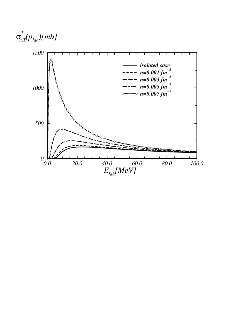
Figure 9: In-medium break-up cross section at $T=10$ MeV. Isolated cross section is shown as solid line. Other lines are due to different nuclear densities.

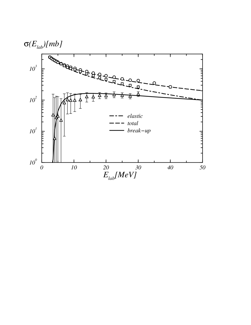
Figure 10: A comparison of the total, elastic, and break-up cross sections $nd\rightarrow nd$, $nd\rightarrow nnp$ with the experimental data of Ref. [18].

From inspection of Fig. 10 we see that the in-medium cross section is significantly enhanced compared to the isolated on. The threshold is shifted to smaller energies, which is because the binding energy of the deuteron becomes smaller. We observe that for higher energies the medium dependence of the cross section becomes much weaker.

Figure 11: Fluctuation time of the deuteron distribution as a function of the deuteron momentum $P$. As input the in-medium cross section is compared to the isolated one, nuclear density $n=0.007$ fm^-3, temperature $T=10$ MeV.

Though the change of the cross section looks dramatic, the quantum Boltzmann equation still has some additional medium dependence that may change this effect in the observables $f_{N}$ and $f_{d}$. Within the linear response theory it is possible to calculate the chemical reaction time due to the break-up process. For small fluctuations $\delta f(t)$ linear response leads to

$$\partial_{t}\delta f_{d}^{\rm reaction}(P,t)=\frac{1}{\tau_{P}}\delta f_{d}^{\rm reaction}(P,t)$$ (21)

where the “life time” of deuteron fluctuations has been introduced,

$$\tau^{-1}_{d}=\frac{4}{3!}\int dk_{N}dk_{1}dk_{2}dk_{3}\;\left|\langle kp|U_{Nd\rightarrow NNN}|k_{1}k_{2}k_{3}\rangle\right|^{2}\;\bar{f}_{1}\bar{f}_{2}\bar{f}_{3}f_{\varepsilon}\;2\pi\delta(E-E_{0}).$$ (22)

which can be related to the break-up cross section given in Eq. 10. For low densities the life time (as a function of the deuteron momentum $P$) and the inverse life time, i.e. the width, at $P=0$ along with the deuteron binding energy for comparison is shown in Fig. 11 [9]. These times have to be compared to the approximate duration of the heavy ion collision of about 200 fm.

5 Conclusion

The treatment of correlations and triple collisions in non-ideal many particle quantum systems opens up a new field for few-body methods. The examples shown have been mostly from nuclear physics. However, applications are possible for stellar plasmas to improve the description of the basic quantity, which is the spectral function and to include correlations into the equation of state. In the laboratory the ionisation rate of dense ionic plasmas is determined by three-particle collisions. A description is presently restricted to hydrogen like plasmas, where the Born approximation for the three-particle reaction is sufficient. Typical applications in nuclear physics are related to heavy ion collisions, here in particular the formation of light clusters such as deuterons, helium-3, tritium, and alpha particles. The conditions are satisfied during the final stage of the heavy ion collision, where a temperature of $T\simeq 5\dots 10$ MeV may be meaningful and the densities are below the Mott densities of cluster formation. The results are also relevant for the equation of states of neutron stars.

The approach given here follows the quantum statistical description as it provides a rigorous, systematic treatment of many particle systems. The major approximation utilized is the cluster expansion to decouple the infinite hierarchy of equations (Green functions or kinetic equations). This approximation clearly goes beyond the quasi particle picture as it includes the residual interactions in a systematic way. This is done rigorously using few-body methods. To this end few-body equations have to be substantially generalized. Presently, these equations resemble an RPA structure [19], however extended to finite temperatures.

The validity of this already ambitious approach has to be checked by facing experimental results. This seems easier for ionic plasmas, e.g. to calculate the ionisation rate, or for electron-hole plasmas in the context of exciton formation. Testing the validity of the approach for nuclear physics needs a handle of heavy ion collisions. Presently one relays on numerical simulations of the complicated dynamics of a heavy ion collision, which is subject to discussions by its own. Typical heavy ion simulation codes that require microscopic input are based on e.g. a Boltzmann-Uehling-Uhlenbeck treatment or on quantum molecular dynamics. The results presented here may however also be relevant for standard nuclear physics, e.g. electron scattering off heavy nuclei, when correlations are considered, and one therefore needs to go beyond the quasi particle picture.

It is a pleasure to thank my colleagues in Rostock who provided me with some material presented during the talk.

References

- [1] D. Pines, R. Tamagaki, S. Tsuruta (editors): The structure and evolution of neutron stars. Reading, MA: Addison-Wesley 1992
- [2] L.P. Kadanoff, G. Baym: Quantum Theory of Many-Particle Systems (Mc Graw-Hill, New York, 1962); A.L. Fetter, J.D. Walecka: Quantum Theory of Many-Particle Systems, (McGraw-Hill, New York, 1971)
- [3] G. Röpke, M. Schmidt, L. Münchow, H. Schulz: Nucl. Phys. A 339 (1983) 587
- [4] A. Schnell, T. Alm, G. Röpke: Phys. Lett. B 387 (1996) 443
- [5] H. Stein, A. Schnell, T.Alm, G. Röpke: Z. Phys. A 351 (1995) 295
- [6] M. Schmidt, G. Röpke, H. Schulz: Ann. Phys. 202 (1990) 57
- [7] M. Beyer, G. Röpke, A. Sedrakian: Phys. Lett. B376 (1996) 7
- [8] E.O. Alt, P. Grassberger, W. Sandhas, Nucl. Phys. B 2 (1967) 167
- [9] M. Beyer, G. Röpke: Phys. Rev. C56 (1997) 2636
- [10] M. Beyer, W. Schadow, C. Kuhrts, G. Röpke: in preparation
- [11] G. Röpke, A. Schnell, P. Schuck, P. Noziéres: Phys. Rev. Lett. 80 (1998) 3177
- [12] T. Alm, G. Chanfray, P. Schuck, G. Welke: Nucl. Phys. A 612 (1997) 472
- [13] D.E. Monakhov, V.B. Belyaev, S.A. Sofianos, S.A. Rakityansky, W. Sandhas: Nucl.Phys. A 635 (1998) 257-269, N.V. Shevchenko, S.A. Rakityansky, S.A. Sofianos, V.B. Belyaev: nucl-th/9804020; S.A. Rakityansky, S.A. Sofianos, L.L. Howell, M. Braun, V. B. Belyaev: Nucl.Phys. A 613 (1997) 132
- [14] T. Bornath, M. Schlanges, F. Morales, R. Prenzel: J. Quant. Radiat. Transfer 58 (1997); T. Bornath, M. Schlanges, R. Prenzel: Phys. Rev. E5 (1998) 1485
- [15] D.N. Zubarev, V.G. Morozow, G. Röpke, Statistical Mechanics of Nonequlibrium Processes Volume 1+2 (Akademie-Verlag, Berlin 1996)
- [16] T. Alm, G. Röpke, W. Bauer, F. Daffin, M. Schmidt, Nucl. Phys. A587 (1995) 815
- [17] P. Danielewicz, G.F. Bertsch, Nucl. Phys. A 533 (1991) 712
- [18] P. Schwarz et al., Nucl. Phys. A 398 (1983) 1
- [19] P. Schuck, Z. Phys. 241 (1971) 395, P. Schuck, F. Villars, P. Ring, Nucl. Phys. A208 (1973) 302, J. Dukelsky, P. Schuck, Nucl. Phys. A512 (1990) 466, P. Schuck, Nucl. Phys. A567 (1994) 78