Abstract

We study theoretically the spin response functions using the relativistic many body theory. The spin response functions in the relativistic theory are reduced largely from the ones of the non-relativistic theory. This happens particularly to the longitudinal spin responses. This fact is able to remove the difficulty in reproducing the ratio of the longitudinal and transverse response functions seen experimentally. We use the local density approximation with the eikonal prescription of the nuclear absorption on the incoming and outgoing nucleons for the calculations of the response functions of finite nuclei. We compare the calculated results with the recent experimental results with $(\vec{p},\vec{n})$ reactions on C and Ca.

PACS : 24.10.Jv, 24.70.+s, 25.40.Kv
keywords : spin response function, relativistic many-body theory, quasielastic reaction

1 Introduction

The spin response functions are very interesting, since they convey directly the informations on the spin correlations among nucleons. The longitudinal spin responses are related with the pionic correlations, which have a strong connection with pion condensation and its precritical phenomenon [1, 2]. The transverse responses are related with the rho mesonic correlations. Due to the mass difference between the pion and the rho meson, the meson exchange force is attractive in the pion channel while it is repulsive in the rho meson channel at medium momenta, $q\sim 2$ fm^-1. Hence the comparison of the two spin responses should reflect this feature directly. In fact, the ratio between the spin responses in these channels was predicted to be largely different from unity [3].

Experiments on the spin responses were performed at LAMPF and RCNP at intermediate energies following the above ideas in mind [4, 5]. The experimental results were found, however, extremely puzzling. The ratios of the longitudinal and the transverse spin responses for various nuclei were found close to or less than one, which is largely different from the theoretical expectations [4, 6]. The surface effects were considered by Esbensen et al., but the ratio could be brought down only to a factor two [7]. Very involved calculations were performed by Ichimura et al. by considering the finite nuclear geometry and the realistic distortion effects [8]. The results were essentially unchanged from that of Esbensen et al..

These results indicate that something essential is missing in the spin correlations among nucleons in nuclei. In this respect, there was a very interesting observation made by several authors [9, 10]. With the use of the pseudovector coupling of the pion with the nucleon instead of the pseudoscalar coupling in the relativistic framework, the pion response becomes much weaker than that of the non-relativistic framework. The pion response function is reduced by a factor $(M^{*}/M)^{2}$ and the effective mass, $M^{*}$ reduces largely in nuclear matter as the density increases in the relativistic many body theory  [11, 12, 13, 14]. Hence, even at the normal matter density without the Landau-Migdal short range correlations, i.e., $g^{\prime}=0$, the pion condensation does not occur [9]. This is a very interesting observation, since this fact largely affects in the longitudinal spin response, which is the pion response, and could be the source to remove the discrepancy.

Horowitz and his collaborators are the ones who apply this idea to the spin response functions and the various spin observables [10]. They found that in fact the ratio could be brought down to close to one in accordance with the experimental observations. These calculations were performed in nuclear matter assuming some typical density representing the nucleus of interest. In this paper, we would like to take into account the change of the densities by considering the hadron distortion effects and compare with the experimental data. In doing so, we would like to compare our results not only with the ratios of the spin responses, but also with the response functions themselves. Particularly, we would like to compare with the recent intensive experimental studies of the $(\vec{p},\vec{n})$ reactions at 400MeV by H. Sakai and his collaborators [6].

This paper consists of the following contents. We write the definition of the response functions and the expressions of the spin response functions in the relativistic framework in Sect.2. We provide the numerical results in Sect.3, where we demonstrate the effects of the relativity on the spin response functions both for the longitudinal and the transverse channels at different densities. We choose here the matter properties calculated by the relativistic mean field theory (RMF) with the non-linear terms with the parameter set TM1 [15]. Sect.4 is devoted to the summary of this work.

2 Spin response functions

Spin response functions have been studied by the $\pi\!+\!\rho\!+\!g^{\prime}$ model in the non-relativistic framework, in which spin longitudinal and spin transverse responses are induced by the residual p-h interactions described in terms of $\pi$ and $\rho$ exchange[16]. The $\pi$ exchange involves the coupling vertex $\mbox{\boldmath$\sigma$}\cdot\mbox{\boldmath$q$}$, hence gives rise to the longitudinal response with respect to momentum transfer $q$, and the $\rho$ exchange involves $\mbox{\boldmath$\sigma$}\!\times\!\mbox{\boldmath$q$}$ which induces the spin transverse response. The relativistic version of the spin responses is described in the Walecka model [11] with the spin dependent interaction Lagrangian [13]

$${\cal L}_{\rm int}=\frac{f_{\pi}}{m_{\pi}}\bar{\psi}_{N}\gamma_{\mu}\gamma_{5}\mbox{\boldmath$\tau$}\psi_{N}\partial^{\mu}\mbox{\boldmath$\pi$}-g_{\rho}\bar{\psi}_{N}(\gamma_{\mu}+\frac{\kappa}{2M}\sigma_{\mu\nu}\partial^{\nu})\mbox{\boldmath$\rho$}_{\mu}\mbox{\boldmath$\tau$}\psi_{N}.$$ (1)

$M$ is the nucleon mass and $\kappa\!=\!6.6$ is the tensor-to-vector ratio in the $\rho NN$ coupling [17]. The $\pi NN$ coupling is assumed to be of the pseudovector representation which incorporates the correct low-energy pion behavior [18].

The first analysis of the spin responses in the relativistic model was done by Horowitz et al., who calculated spin observables [10]. Our goal is to reveal the relativistic effects on the spin response functions and compare with the experimental cross sections observed in $(\vec{p},\vec{n})$ reactions on finite nuclei, with nuclear distortion effect taken into account. The spin response functions are obtained by taking the imaginary part of the polarization functions induced by the interaction Lagrangian (1) as functions of the 4-momentum transfer $q=(\omega,\vec{q})$. For nuclear matter the pseudovector and $\rho$ meson induced polarization functions in the lowest order are given as

$$i\Pi_{\rm PV}(q) = {\rm Tr}\int\frac{d^{4}k}{(2\pi)^{4}}\gamma_{5}\!\,{\not{\!q}}\mbox{\boldmath$\tau$}_{1}G(k+q)\gamma_{5}\!\,{\not{\!q}}\mbox{\boldmath$\tau$}_{2}G(k)$$ (2)

$$i\Pi_{\mu\nu}(q) = {\rm Tr}\int\frac{d^{4}k}{(2\pi)^{4}}\Gamma_{\mu}\mbox{\boldmath$\tau$}_{1}G(k+q)\bar{\Gamma}_{\nu}\mbox{\boldmath$\tau$}_{2}G(k)$$ (3)

where $\Gamma_{\mu}\!=\!\gamma_{\mu}\!-\!i\frac{\kappa}{2M}\sigma_{\mu\nu}q^{\nu}$($\bar{\Gamma}_{\mu}\!=\!\gamma_{\mu}\!+\!i\frac{\kappa}{2M}\sigma_{\mu\nu}q^{\nu}$). $G(k)$ is the nucleon Green’s function,

$$G(k) = G_{F}(k)+G_{D}(k)$$

$$G_{F}(k)=(\!\,{\not{\!\bar{k}}}+M^{*})g_{F}(k), G_{D}(k)=(\!\,{\not{\!\bar{k}}}+M^{*})g_{D}(k)$$

$$g_{F}(k)=\frac{1}{\bar{k}^{2}-M^{*2}+i\eta}, g_{D}=\frac{i\pi}{\epsilon_{k}}\delta(\bar{k}_{0}-\epsilon_{k})\theta(\epsilon_{F}-\bar{k}_{0})$$

$$\bar{k} = (k_{0}-\Sigma_{V},\mbox{\boldmath$k$})$$

$$\epsilon_{k} = \sqrt{\mbox{\boldmath$k$}^{2}+M^{*2}}.$$

$\epsilon_{F}$ denotes the Fermi energy, $\epsilon_{F}=\sqrt{k_{F}^{2}+M^{*2}}$, with $k_{F}$ the Fermi momentum. $M^{*}=\!M+\Sigma_{S}$ is the nucleon effective mass given by the relativistic mean field theory with $\Sigma_{S},\Sigma_{V}$ being the scalar and vector potentials. The transverse polarization $\Pi_{T}$ is obtained by projecting $\Pi_{\mu\nu}$ onto the plane perpendicular to $q$ [19]. Thus

$$\Pi_{L} = \Pi_{\rm PV}$$

$$\Pi_{T} = (\frac{q_{0}^{2}}{\mbox{\boldmath$q$}^{2}}\Pi_{00}+\Pi^{i}_{\,\,i})/2.$$ (4)

In the calculation of the polarization functions, we neglect the vacuum polarization of the form $\int\frac{d^{4}k}{(2\pi)^{4}}\Gamma G_{F}\Gamma G_{F}$ which represents the coupling of the meson to $N\bar{N}$.

The vector current conservation relation, $q_{\mu}\bar{\psi}\gamma^{\mu}\psi=0$, allows us to reduce $\Pi_{\rm PV}(q)$ to  [20]

$$i\Pi_{\rm PV}=-16M^{*2}q^{2}\int\frac{d^{4}k}{(2\pi)^{4}}g(k)g(k+q)$$ (5)

where $g(k)=g_{F}(k)+g_{D}(k)$. $\Pi_{L}$ is written with $I_{0}(q)$ in  [21] as

$$\Pi_{L}=4M^{*2}q^{2}I_{0}.$$ (6)

The explicit form of $Im\Pi_{L}$ is given as

$$Im\Pi_{L}=\frac{M^{*2}q^{2}}{\pi\mid\!\mbox{\boldmath$q$}\!\mid}\left\{\begin{array}[]{cc}\omega&(k_{+}<k_{F})\\ \epsilon_{F}-\epsilon_{k_{-}}&(\mid\!\!k_{-}\!\!\mid<k_{F}<k_{+})\\ 0&(k_{F}<\mid\!\!k_{-}\!\!\mid)\end{array}\right.$$ (7)

and the real part is given as

$$Re\Pi_{L} = \frac{M^{*2}q^{2}}{\pi\mid\!\mbox{\boldmath$q$}\!\mid}\left\{\epsilon_{F}\ln{\left|\frac{(k_{F}-k_{+})(k_{F}-k_{-})}{(k_{F}+k_{+})(k_{F}+k_{-})}\right|}-2\omega\ln{\frac{k_{F}+\epsilon_{F}}{M^{*}}}\right.$$

$$- \left.\left(\epsilon_{k_{+}}+\ln{\left|\frac{(M^{*2}+k_{+}k_{F}-\epsilon_{k_{+}}\epsilon_{F})(k_{F}+k_{+})}{(M^{*2}-k_{+}k_{F}-\epsilon_{k_{+}}\epsilon_{F})(k_{F}-k_{+})}\right|}+(k_{+}\rightarrow k_{-})\right)\right\}$$

with

$$k_{\pm}=\frac{\mid\!\mbox{\boldmath$q$}\!\mid}{2}\pm\frac{\omega}{2}\sqrt{1-\frac{4M^{*2}}{q^{2}}}.$$

On the other hand, $\Pi_{T}$ is divided into three components, each of which originates from the vector-vector, vector-tensor and tensor-tensor contributions,

$$\Pi_{T}=\Pi_{v}+\Pi_{v,t}+\Pi_{t},$$ (9)

$$\Pi_{v} = \frac{1}{2}\left[(4M^{*2}+q^{2})I_{0}+\frac{q^{2}}{\mbox{\boldmath$q$}^{2}}I_{2}\right]+\frac{\omega^{2}+\mbox{\boldmath$q$}^{2}}{2\mbox{\boldmath$q$}^{2}}\frac{\rho_{s}}{M^{*}}$$ (10)

$$\Pi_{v,t} = 4\frac{\kappa}{2M}M^{*}q^{2}I_{0}$$ (11)

$$\Pi_{t} = \left(\frac{\kappa}{2M}\right)^{2}q^{2}\left[(4M^{*2}+q^{2})I_{0}-\frac{q^{2}}{\mbox{\boldmath$q$}^{2}}I_{2}-\frac{q^{2}}{\mbox{\boldmath$q$}^{2}}\frac{\rho_{s}}{M^{*}}\right].$$ (12)

$\rho_{s}$ is the scalar density and $I_{0}$ and $I_{2}$ are given in  [21], where the response functions in $(e,e^{\prime})$ inelastic scattering were calculated.

In order to define the response functions in the relativistic model, it is necessary to consider the non-relativistic limit of the vertex operators since all the discussions have been made in the non-relativistic framework. While $\gamma_{5}\gamma_{\mu}q^{\mu}\rightarrow\mbox{\boldmath$\sigma$}\cdot\mbox{\boldmath$q$}$,

$$\gamma_{\mu}-i\frac{\kappa}{2M}\sigma_{\mu\nu}q^{\nu}\rightarrow\frac{\kappa+1}{2M}\mbox{\boldmath$\sigma$}\!\times\!\mbox{\boldmath$q$},$$ (13)

in the non-relativistic reduction. Thus, we define the relativistic response functions $R_{L}$, $R_{T}$ by

$$q^{2}R_{L} = \frac{1}{\pi\rho}Im\Pi_{L}$$ (14)

$$\left(\frac{\kappa+1}{2M}\right)^{2}q^{2}R_{T} = \frac{1}{\pi\rho}Im\Pi_{T},$$ (15)

where $\rho$ is the nuclear density. They correspond to the response functions in non-relativistic model $R_{\rm NR}$ defined by

$$\mbox{\boldmath$q$}^{2}R_{\rm NR}=-\frac{1}{\pi\rho}Im\Pi_{\rm NR}$$ (16)

where $\Pi_{\rm NR}$ are the non-relativistic polarization functions for the vertex operators, $\mbox{\boldmath$\sigma$}\cdot\mbox{\boldmath$q$}$ or $\mbox{\boldmath$\sigma$}\!\times\!\mbox{\boldmath$q$}$. We remind you that in the non-relativistic model the longitudinal response and the transverse response are identical for the symmetric nuclear matter and they are expressed by the Lindhard function given in  [22].

Here we give an overview of the relativistic responses in comparison with the non-relativistic ones. First we discuss the longitudinal response functions. In the high density case where $k_{F}$ is large, the bulk part of the response function is given by the linear term in $\omega$, the first row in Eq.(7). A typical case is shown in Fig.1. We find that in the linearly $\omega$-depending region we gain an exact relation, $R_{L}=\left(\frac{M^{*}}{M}\right)^{2}\!R_{\rm NR}$. In the low density case where $k_{F}$ is small, most part of the response function is represented by the second row in Eq.(7). This expression differs from the non-relativistic response only in the relativistic kinematics and the effective mass. We find that at the peak position $\omega=\sqrt{\mbox{\boldmath$q$}^{2}+M^{*2}}-M^{*}$ obtained by setting $k_{-}\!=0$ in Eq.(7), $-Im\Pi_{L}=-\frac{M^{*2}q^{2}}{\pi\mid\mbox{\boldmath$q$}\mid}(\epsilon_{F}-M^{*})\approx-\frac{M^{*}k_{F}^{2}q^{2}}{2\pi\mid\mbox{\boldmath$q$}\mid}$ shows approximately linear dependence on the effective mass. In the non-relativistic limit with $M^{*}=M$ this can be reduced to the non-relativistic case which provides the peak position $\omega=\frac{\mbox{\boldmath$q$}^{2}}{2M}$ and the peak height $-Im\Pi_{\rm NR}=\frac{Mk_{F}^{2}\mbox{\boldmath$q$}^{2}}{2\pi\mid\mbox{\boldmath$q$}\mid}$. This implies that the relativistic responses are reduced by a factor $\left(\frac{M^{*}}{M}\right)^{2}$ at higher density and by $\frac{M^{*}}{M}$ at lower density compared with the non-relativistic one at the same density.

Second we discuss the transverse response. $\Pi_{T}$ is rather complicated to make a clear and brief analysis over all $\omega$ region. Hence, we analyze here the high density case where at lower $\omega$

$$ImI_{0} = \frac{\omega}{4\pi\mid\mbox{\boldmath$q$}\mid}$$ (17)

$$ImI_{2} = \frac{1}{12\pi\mid\mbox{\boldmath$q$}\mid}(12(M^{*2}+k_{F}^{2})\omega+\omega^{3})$$ (18)

$$\approx 4(M^{*2}+k_{F}^{2})ImI_{0}.$$ (19)

The leading order of $ImI_{0}$ and $ImI_{2}$ in $M^{*}$ yields

$$Im\Pi_{T} \approx \left[-2k_{F}^{2}+\frac{1}{2}q^{2}+2\kappa\frac{M^{*}}{M}q^{2}+\kappa^{2}\left(\frac{M^{*}}{M}\right)^{2}q^{2}\right]ImI_{0}$$ (20)

$$\sim \left(1+\kappa\frac{M^{*}}{M}\right)^{2}q^{2}ImI_{0}.$$ (21)

We can find by considering the definition Eq.(14) that setting $M^{*}=M$ makes $R_{T}$ approximately agree with $R_{L}$ and therefore with $R_{NR}$. Pay attention to the fact that $R_{T}$ depends on $M^{*}$ in more moderate way than $R_{L}$. This arises from the vector-tensor mixed coupling of $\rho$ to nucleons; the trace appearing in the calculation of $\Pi_{v,t}$ in Eq.(3) does not give rise to $M^{*2}$ term, i.e., $Tr[\gamma_{\mu}(\,{\not{\!k}}+\,{\not{\!q}}+M^{*})\sigma_{\nu\lambda}(\,{\not{\!k}}+M^{*})]q^{\lambda}=4M^{*}(g_{\mu\nu}q^{2}-q_{\mu}q_{\nu})$ due to the vanishing traces of product of odd numbers of Dirac $\gamma$ matrices, while $M^{*2}$ term appears in the other. This leads to $R_{L}/R_{T}$ smaller than unity with $M^{*}/M<1$ as illustrated in Fig.1 where $R_{L}$ is found smaller than $R_{T}$ in the whole $\omega$ region. We see clearly the difference between $R_{L}$ and $R_{T}$. Here, we have used the effective nucleon mass $M^{*}$ by using the relativistic mean field theory as explained in the numerical calculation section.

In order to incorporate higher order correction by the $\pi$ and $\rho$ exchange interaction, we carry out the random phase approximation which sums up ring diagrams to all orders and is expressed by Dyson’s equation

$$\Pi^{\rm RPA}=\Pi^{0}+\Pi^{0}V\Pi^{\rm RPA}.$$ (22)

$\Pi^{0}$ is the free response function defined above and $\Pi^{\rm RPA}$ is the full response function obtained by RPA. $V$ is $\pi$ and $\rho$ meson exchange interaction,

$$V_{\pi}(q) = \left(\frac{f_{\pi}}{m_{\pi}}\right)^{2}\left(\frac{1}{q^{2}-m_{\pi}^{2}}-\frac{g^{\prime}_{\pi}}{q^{2}}\right)$$ (23)

$$V_{\rho}^{\mu\nu}(q) = g_{\rho}^{2}(g^{\mu\nu}-q^{\mu}q^{\nu}/m_{\rho}^{2})\left(\frac{1}{q^{2}-m_{\rho}^{2}}-C_{\rho}^{-1}\frac{g^{\prime}_{\rho}}{q^{2}}\right).$$ (24)

$C_{\rho}=2.18$ is the ratio of couplings of non-relativistic interactions $\left(\frac{f_{\rho}}{m_{\rho}}\right)^{2}/\left(\frac{f_{\pi}}{m_{\pi}}\right)^{2}$ and $g^{\prime}_{\pi}$ and $g^{\prime}_{\rho}$ are ’relativistic’ phenomenological Landau-Migdal parameters introduced to take into account short range nuclear correlations. In reality the RPA equation for the polarization function induced by the $\rho$ exchange involves Lorentz contraction. We can, however, deduce the RPA equation to the same form as that for $R_{L}$ by consideration that $q^{\mu}\Pi_{\mu\nu}=0$ and decomposition, $\Pi_{\mu\nu}=P^{L}_{\mu\nu}\Pi_{L}^{(\rho)}+P^{T}_{\mu\nu}\Pi_{T}^{(\rho)}$. Here $P^{L,T}_{\mu\nu}$ are projection operators which extract the longitudinal and transverse part $\Pi_{L,T}^{(\rho)}$ of the $\rho$-induced response[19]. Finally we obtain the RPA response functions in a simple form,

$$\Pi_{L}^{\rm RPA} = (1-V_{\pi}\Pi_{L}^{0})^{-1}\Pi_{L}^{0}$$ (25)

$$\Pi_{T}^{\rm RPA} = (1-V_{\rho}\Pi_{T}^{0})^{-1}\Pi_{T}^{0}$$ (26)

with

$$V_{\rho}(q)=g_{\rho}^{2}\left(\frac{1}{q^{2}-m_{\rho}^{2}}-C_{\rho}^{-1}\frac{g^{\prime}_{\rho}}{q^{2}}\right).$$ (27)

We adopt $g_{\rho}=2.6$ which satisfies

$$\frac{f_{\rho}}{m_{\rho}}\approx g_{\rho}\frac{\kappa+1}{2M},$$ (28)

in accordance with the non-relativistic coupling constant.

The Landau-Migdal parameter was originally introduced in the non-relativistic $\pi\!+\!\rho\!+\!g^{\prime}$ model and in that case the non-relativistic Landau-Migdal parameter is $g^{\prime}=g^{\prime}_{\pi}\!=\!g^{\prime}_{\rho}$, since

$$V_{g^{\prime}} = g^{\prime}\left(\frac{f_{\pi}}{m_{\pi}}\right)^{2}\mbox{\boldmath$\sigma$}_{1}\!\cdot\!\mbox{\boldmath$\sigma$}_{2}\,\mbox{\boldmath$\tau$}_{1}\!\cdot\!\mbox{\boldmath$\tau$}_{2}$$ (29)

$$= g^{\prime}\left\{\left(\frac{f_{\pi}}{m_{\pi}}\right)^{2}\mbox{\boldmath$\sigma$}_{1}\!\cdot\!\hat{q}\,\mbox{\boldmath$\sigma$}_{2}\!\cdot\!\hat{q}+\left(\frac{f_{\rho}}{m_{\rho}}\right)^{2}C_{\rho}^{-1}\mbox{\boldmath$\sigma$}_{1}\!\times\!\hat{q}\cdot\mbox{\boldmath$\sigma$}_{2}\!\times\!\hat{q}\right\}\mbox{\boldmath$\tau$}_{1}\!\cdot\!\mbox{\boldmath$\tau$}_{2}.$$

$g^{\prime}=0.6\sim 0.7$ is usually used as a standard value. On the other hand, the longitudinal correlation $g^{\prime}_{\pi}$ and the transverse correlation $g^{\prime}_{\rho}$ defined in Eqs.(23) and (24) are in general different. It is very interesting to extract these informations from the G-matrix of the relativistic Brückner-Hartree-Fock theory[23]. Here, we extract them from inelastic electron scattering experiments. Horowitz et.al. studied the transverse response involved with $(e,e^{\prime})$ scattering[10], from which they obtained $g^{\prime}_{\rho}=0.3$ to reproduce the data. As for $g^{\prime}_{\pi}$, we choose the conventional value, $g^{\prime}_{\pi}=0.7$. Thus we employ here the parameter set $g^{\prime}_{\rho}=0.3,g^{\prime}_{\pi}=0.7$.

In (p,n) reactions the distortion effect is of much importance compared with $(e,e^{\prime})$ reactions due to large nucleon-nucleon cross section, $\sigma_{NN}$. We carry out the local density approximation with the attenuation factor given by the eikonal approximation to obtain the $(\vec{p},\vec{n})$ cross sections by using the nuclear matter calculation. The response functions for finite nucleus are expressed by

$$R^{\rm LDA}_{T,L}=\frac{1}{N_{\rm eff}}\frac{N}{A}\int 2\pi b\,db\,dze^{-\chi(b)}\rho(b,z)R_{T,L}(k_{F}).$$ (30)

$e^{-\chi(b)}$ is the attenuation factor for the reaction with the impact parameter $b$ where $\chi(b)=\int_{-\infty}^{+\infty}dz\sigma_{NN}\rho(b,z)$. $\rho(b,z)$ is the nuclear density profile of the target nucleus in the cylindrical coordinate. The effective neutron number $N_{\rm eff}$ is given as the normalization factor

$$N_{\rm eff} = \frac{N}{A}{\int 2\pi b\,db\,dze^{-\chi(b)}\rho(b,z)}$$ (31)

$$= \frac{N}{A}\frac{1}{\sigma_{NN}}\int 2\pi b\,db\,\chi(b)e^{-\chi(b)}.$$

Here the factor $\frac{N}{A}$ appears for the use of the neutron density instead of nucleon density in Eq.(30),(31). For the nuclear density distribution $\rho(\mbox{\boldmath$r$})$ we adopt the three-parameter Fermi-type form determined experimentally [24]. The response function $R(k_{F})$ is obtained by the nuclear matter calculation using the Fermi momentum and the effective mass given by the relativistic mean field calculation for nuclear matter [14], at the corresponding density. We use $\sigma_{NN}\!=\!30$mb which is close to the free cross section at the relevant energy $T_{\rm lab}\approx 400$MeV, since the reaction is supposed to take place close to the nuclear surface. The typical Fermi momentum $\bar{k}_{F}$ is obtained by replacing $R(\rho(b,z))$ in Eq.(30) by $k_{F}\sim\rho^{1/3}$. We find $\bar{k}_{F}=0.98(0.97)$ for ¹²C(⁴⁰Ca) with $M^{*}$ at this density being $M^{*}=0.82(0.83)M$.

3 Numerical results

We show the numerical results on the response functions at $\mid\!\mbox{\boldmath$q$}\!\mid=\!1.7$fm^-1 which are of special interest here and measured by the experiments. To begin with we demonstrate relativistic effects on free response functions of nuclear matter at different densities. In Fig.1 we show the free response functions for the symmetric nuclear matter at the saturation density $k_{F}\!=\!1.36$fm^-1, with the effective mass $M^{*}\!=\!0.59M$ which is given by the RMF calculation. For comparison the non-relativistic response function and the relativistic response with $M^{*}\!=\!M$ are also shown in the figure. We see that the longitudinal spin response $R_{L}$ with $M^{*}\!=\!0.59M$ is reduced from the non-relativistic response due to the effect of the effective mass. This is affirmed by seeing that $R_{L}$ becomes close to $R_{\rm NR}$ by setting $M^{*}\!=\!M$, which are, as stated in the previous section, identical with $R_{\rm NR}$ for $\omega<30$MeV. Broadening of the width is a consequence of enlarged maximum particle-hole excitation energy for given momentum transfer $\sqrt{(k_{F}+\mid\!\mbox{\boldmath$q$}\!\mid)^{2}+M^{*2}}-\sqrt{k_{F}^{2}+M^{*2}}\sim\frac{k_{F}\mid\mbox{\boldmath$q$}\mid}{M^{*}}$. We find the transverse response $R_{T}$ shows more moderate effective mass dependence, and it is larger than the longitudinal response with the same effective mass. We mention here that the effective mass also makes the non-relativistic responses smaller as the case of the relativistic responses[25, 26, 27]. There are, however, two major differences between the relativistic and the non-relativistic cases. First, the effective mass is much smaller for the relativistic case. Second, while the effective mass effect works in the same way for both the spin longitudinal and the transverse responses in the non-relativistic case, in the relativistic case, the longitudinal response is more reduced than the transverse one as shown here and in the previous section. As a result we find the ratio $R_{L}/R_{T}\approx 0.8$ with little dependence on $\omega$.

In Fig.2 the free response functions for $k_{F}=0.97$fm^-1($M^{*}\!=\!0.83$) are shown, which corresponds to the density $\rho=0.37\rho_{0}$. $(\vec{p},\vec{n})$ reaction is supposed to take place in the surface region of a nucleus with about this density because of the large distortion of the incident and outgoing nucleon. The width becomes narrower and the magnitude becomes larger than those at the saturation density due to the small Fermi momentum and the larger effective mass. The qualitative features in the previous figure hold also true here. The difference between $R_{L}$ and $R_{T}$ is also smaller than Fig.1, which yields $R_{L}/R_{T}\approx 0.94$. We find that in any case $R_{L}/R_{T}<1$ holds in the relativistic case. This fact is crucial to reproduce the experimental observation $R_{L}/R_{T}\approx 1$.

Next we show the relativistic responses calculated by RPA. In Fig.3(a) we show the longitudinal responses with RPA at the saturation density together with free response and compare with the non-relativistic results. We see that the relativistic response with RPA correlation , $R_{L}^{\rm RPA}$, is only slightly enhanced by the attractive $\pi$ exchange interaction while the non-relativistic one is largely enhanced. The difference from the non-relativistic case originates from the effective coupling reduced by the factor $\left(\frac{M^{*}}{M}\right)^{2}$ which makes $R_{L}^{\rm RPA}$ closer to the free response, $R_{L}^{\rm RPA}\sim R_{L}^{\rm Free}$. In Fig.3(b), on the other hand, we show the transverse responses at the same density. It is found that the relativistic response with RPA, $R_{T}^{\rm RPA}$, almost agrees with the free response. This arises from $V_{\rho}\approx 0$ with $g^{\prime}_{\rho}\!=\!0.3$, while the non-relativistic response is considerably quenched by the repulsive $\rho$ exchange force with $g^{\prime}\!=\!0.7$. We find that the reduction of the relativistic longitudinal response compared with the transverse response is compensated by the RPA correlation. It follows that $R_{L}^{\rm RPA}/R_{T}^{\rm RPA}\approx 1$ at low $\omega$(Fig.5). It is in good contrast with the non-relativistic case where significant quenching of the transverse response and enhancement of the longitudinal one is found to yield $R_{L}^{\rm RPA}/R_{T}^{\rm RPA}\gg 1$.

We note here that the use of the smaller ’relativistic’ $g^{\prime}_{\rho}$ in the transverse channel is supported by the similarity of the transverse responses, $R_{T}^{\rm RPA}$, shown by the solid curve and by the thin dotted line curve in the smaller $\omega$ region in Fig.3(b). The relativistic free response is already reduced largely from the non-relativistic one.

In Fig.4(a), (b) we show the responses with RPA at $k_{F}\!=\!0.97$fm^-1. The dependence of $R^{\rm free}$ on $k_{F}$ causes the attractive $\pi$ exchange force weaker in both the non-relativistic and relativistic cases. In the latter case the factor $\frac{M^{*}}{M}$ reduces still more the effective coupling, hence less enhancement by RPA correlation. The relativistic transverse response $R_{T}^{\rm RPA}$ agrees with the free response for the same reason as in the case of the saturation density. We obtain the ratio $R_{L}^{\rm RPA}/R_{T}^{\rm RPA}=1\sim 1.2$ at low $\omega$, while the non-relativistic case results in $R_{L}^{\rm RPA}/R_{T}^{\rm RPA}>2$ with striking $\omega$ dependence as shown in Fig.5. The relativistic results are in agreement with the experimental situation.

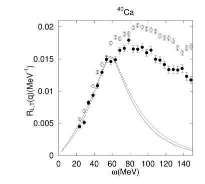
Figure 6: Response functions with RPA(upper panels) and ratio of the longitudinal to the transverse response(lower panels) at $\mid\!\mbox{\boldmath$q$}\!\mid=1.7$fm^-1 obtained by the local density approximation with $\sigma_{NN}=30$mb for ¹²C(left panels) and ⁴⁰Ca(right panels). In the upper panels the longitudinal response is drawn by a solid curve and the transverse by a dashed curve. The experimental data are plotted by solid circles for the longitudinal response and by open circles for the transverse one. The experimental responses are multiplied by a factor $N_{\rm eff}^{\rm exp}/N_{\rm eff}$(see the text). In the lower panels the theoretical value is drawn by a solid curve and the experimental data are plotted by solid circles with error bars.

Finally we compare the results obtained by the local density approximation with the experimental data recently measured at RCNP [6]. Fig.6 shows the results on ¹²C(the left panels) and ⁴⁰Ca(the right panels). The in-medium cross section $\sigma_{NN}\!=\!30$mb provides effective neutron number $N_{\rm eff}\!=\!2.0(3.7)$ for ¹²C(⁴⁰Ca). Since our effective neutron number differs from the experimental one, we multiply $N_{\rm eff}^{\rm exp}/N_{\rm eff}$ to the experimental data where $N_{\rm eff}^{\rm exp}$ is the effective neutron number adopted in the experimental analysis, $N_{\rm eff}^{\rm exp}=2.7$(6.0) for ¹²C and ⁴⁰Ca, respectively. This is because the “experimental” response functions extracted from the cross sections and the polarization measurements by the experimentalists were obtained by dividing the corresponding quantities with $N_{\rm eff}^{\rm exp}$[4, 6]. On the other hand, the “theoretical” response functions are obtained by dividing the corresponding quantities with $N_{\rm eff}$ as shown in Eq.(30). As seen in the discussion above about the matter properties, the longitudinal and the transverse responses are very close to each other. Below $\omega<60$MeV, the theoretical results are close to the experimental responses (The use of smaller in-medium cross section $\sigma_{NN}$ makes the agreement better in ¹²C). However, the theoretical responses are much smaller than the experimental results above $\omega>60$MeV. For the full understanding of the problem of the spin response functions, we have to describe this deviation. The $\Delta$ excitation starts to contribute above $\omega>80$MeV as can be seen from the $(e,e^{\prime})$ data[10]. It would be very interesting to work out the two and multiple scattering processes in the $(p,p^{\prime})$ and $(p,n)$ reactions for the spin responses[28].

4 Conclusion

We have studied the relativistic effects on the spin response functions by using the relativistic version of the $\pi\!+\!\rho\!+\!g^{\prime}$ model. We have calculated the polarization functions in the $\pi$(spin longitudinal) channel and $\rho$ meson(spin transverse) channel in the nuclear medium to obtain the spin response functions. We have adopted the pseudovector coupling for $\pi NN$ channel instead of the pseudoscalar coupling. The longitudinal response calculated with the pseudovector coupling is largely reduced by the effective mass which is $\frac{M^{*}}{M}=0.6\sim 0.8$ in the nuclear medium. The reduction factor is found to be $\left(\frac{M^{*}}{M}\right)^{2}$ at the higher density and $\frac{M^{*}}{M}$ at the lower density. On the other hand the transverse response is reduced by $\left(1+\kappa\frac{M^{*}}{M}\right)^{2}/(1+\kappa)^{2}$ at the high density because of the vector-tensor coupling for $\rho NN$ vertex. We have found that the relativistic longitudinal and transverse responses agree with the non-relativistic ones in the case of $M^{*}=M$. We have shown that without RPA correlation the longitudinal response is less than the transverse response even at the low density because of the different effective mass dependence.

The reduction of the effective mass also reduces the higher order $\pi NN$ and $\rho NN$ correlations in the medium. We have demonstrated that the relativistic longitudinal response function is enhanced much less than the non-relativistic case by the attractive $\pi$ exchange force. The transverse response with RPA correlation has been calculated with the Landau-Migdal parameter $g^{\prime}_{\rho}=0.3$, which is chosen by Horowitz et al. as a fitting parameter in the analysis of electron scattering. We have shown that the transverse response is hardly affected by RPA. As a result we have obtained similar response functions for the longitudinal and the transverse spin responses. It is in agreement with the experimental data at least in the small $\omega$ region, which is qualitatively different from the non-relativistic theoretical results.

We have calculated the response functions for ¹²C and ⁴⁰Ca by using the eikonal prescription for the distortion effect with the use of the response functions in nuclear matter. We have compared the longitudinal and the transverse response functions directly with the recently obtained experimental results. We see close reproductions of the spin responses in the small $\omega$ region($\omega<60$MeV) for both the longitudinal and the transverse channels. The result is due largely to the use of the relativistic responses with the pseudovector coupling in the $\pi$ channel with large reduction of the effective nucleon mass in the nuclear medium. The use of the smaller $g^{\prime}_{\rho}$($g^{\prime}_{\rho}=0.3$) is adopted for another reason. This small value is extracted from $(e,e^{\prime})$ reactions phenomenologically and needs to be studied theoretically in the relativistic G-matrix theory.

The theoretical responses underestimate the experimental ones largely above $\omega>60$MeV. We expect two and more step processes at this high excitation energies, which should be worked out quantitatively. We start to see the effect of the $\Delta$ isobar excitations already starting around $\omega>80$MeV, which are seen in the $(e,e^{\prime})$ reaction data. Unless these effects are quantitatively studied, our theoretical results discussed in this paper is considered as a plausible explanation of the long standing puzzle on the ratios of the longitudinal and the transverse responses.

Figure 1: Free relativistic longitudinal response function $R_{L}$ (thick solid curve) and transverse response function $R_{T}$ (thick dashed) and non-relativistic one $R_{\rm NR}$ (thin solid) at $\mid\!\!\mbox{\boldmath$q$}\!\!\mid=\!1.7$fm^-1 for the symmetric nuclear matter as functions of the excitation energy $\omega$ at the saturation density with the Fermi momentum, $k_{F}\!=\!1.36$fm^-1. For comparison the relativistic longitudinal response with $M^{*}\!=\!M$ is shown(thin dashed).

Figure 2: Same as Fig.1 for $k_{F}=0.97$fm^-1 which corresponds to the typical density of the nucleus in $(p,n)$ reaction because of the large distortion effects on the incident and outgoing nucleons.

Figure 3: (a)Longitudinal and (b)transverse responses with and without RPA correlation at the saturation density,$k_{F}=1.36$fm^-1. Thick solid curves indicate the relativistic free responses $R_{L}^{\rm free}$ and $R_{T}^{\rm free}$ and thick dashed curves RPA results $R_{L}^{\rm RPA}$ and $R_{T}^{\rm RPA}$. The corresponding non-relativistic values are drawn with thin solid and dashed curves.

Figure 4: Same as Fig.3 for $k_{F}=0.97$fm^-1.

Figure 5: Ratio of the longitudinal response to the transverse one with RPA at the saturation density and $k_{F}=0.97$fm^-1corresponding to $\rho=0.37\rho_{0}$. A thick solid curve indicates the relativistic result at the saturation density and a thick dashed curve for $k_{F}=0.97$fm^-1. Thin solid and dashed curves indicate the non-relativistic results at the saturation density and at $\rho=0.37\rho_{0}$, respectively.

References

• [1] A.B. Migdal, Rev. Mod. Phys. 50(1978)107 and references therein.
• [2] H. Toki and W. Weise, Phys. Rev. Lett. 42(1979)1034.
• [3] W.M. Alberico, M. Ericson and A. Molinari, Nucl. Phys. A379(1982)429.
• [4] T.A. Carey, K.W. Jones, J.B. McClelland, J.M. Moss, L.B. Rees, N. Tanaka and A.D. Bacher, Phys. Rev. Lett. 53(1984)144.
L.B. Rees, J.M. Moss, T.A. Carey, K.W. Jones, J.B. McClelland, N. Tanaka, A.D. Bacher and H. Esbensen, Phys. Rev. C34(1986)627.
J.B. McClelland et al., Phys. Rev. Lett. 69(1992)582.
X.Y. Chen et.al, Phys. Rev. C47(1993)2159.
T.N. Taddeucci et al., Phys. Rev. Lett. 73(1994)3516.
• [5] H. Sakai, M.B. Greenfield, K. Hatanaka, S. Ishida, N. Koori, H. Okamura, A. Okihana, H. Otsu, N. Sakamoto, Y. Satou, T. Uesaka and T. Wakasa, Nucl. Phys. A577(1994)111c.
• [6] T. Wakasa et al., submitted to Phys. Rev. C.
T. Wakasa, private communication.
• [7] H. Esbensen, H. Toki and G. Bertsch, Phys. Rev. C31(1985)1816.
• [8] M. Ichimura, K. Kawahigashi, T.S. JΓΈrgensen and C. Gaarde, Phys. Rev. C39(1989)1446.
• [9] B.L. Birbrair, V.N. Fomenko and L.N. Savushkin, J. Phys. G8(1982)1517.
• [10] C.J. Horowitz and J. Piekarewicz, Phys.Lett. B301(1993)321.
C.J. Horowitz and J. Piekarewicz, Phys.Rev. C50(1994)2540.
• [11] J.D. Walecka, Ann. Phys. 83(1974)491.
• [12] B.D. Serot and J.D. Walecka, Adv. in Nucl.Phys. 16(1986).
• [13] R. Brockmann and R. Machleidt, Phys. Rev. C42(1990)1965.
• [14] D. Hirata ,H. Toki, T. Watabe, I. Tanihata and B.V. Carlson, Phys. Rev. C44(1991)1467.
• [15] Y. Sugahara and H. Toki, Nucl. Phys. A579(1994)557.
• [16] E. Oset, H. Toki and W. Weise, Phys. Rep. 83(1982)281.
• [17] G. HΓΆhler and E. Pietarinen, Nucl. Phys. B95(1975)210.
• [18] T. Matsui and B.D. Serot, Ann. Phys. 144(1982)107.
• [19] H. Shiomi and T. Hatsuda, Phys.Lett. B334(1994)281.
• [20] J.F. Dawson and J. Piekarewicz, Phys. Rev. C43(1991)2631.
• [21] H. Kurasawa and T. Suzuki, Nucl. Phys. A445(1985)685.
• [22] A.L. Fetter and J.D. Walecka, Quantum theory of many-particle systems (McGraw-Hill, New York, 1971).
• [23] C. Fuchs, L. Sehn and H.H. Wolter, Nucl. Phys. A601(1996)505.
• [24] C.W. de Jager, H. de Vries and C. de Vries, At. Data Nucl. Data Tables 14(1974)479.
• [25] H. Toki, Y. Futami and W. Weise, Phys. Lett. B78(1978)547.
• [26] W.H. Dickhoff, A. Faessler, H. Muther and J. Meyer-Ter-Vehn, Nucl. Phys. A368(1981)445.
W.H. Dickhoff, A. Faessler, J. Meyer-Ter-Vehn and H. Muther, Phys. Rev. C23(1981)1154.
• [27] E. Shiino, Y. Saito, M. Ichimura and H. Toki, Phys. Rev. C34(1986)1004.
• [28] A. De Pace, Phys. Rev. Lett. 75(1995)29.
Refer to caption