Classical Quark Models:
An Introduction

Abstract

We present an elementary introduction to some of the quark models used to understand the properties of light mesons and baryons. These lectures are intended for both theoretical and experimental graduate students beginning their study of the strong interaction.

1 Introduction

Modern nuclear and particle physics has a secure theoretical foundation based on the idea of local gauge invariance, known as the standard model. It has satisfied every experimental or theoretical challenge directed at it so far. In the electroweak sector it was spectacularly confirmed by the discovery of the heavy vector bosons (the $W^{\pm}$ and $Z^{0}$) in the early 80’s. On the other hand, in the strong interaction sector, quantum chromodynamics (QCD) has presented more problems. While it has passed every test in the regions where it can be solved (notably the QCD evolution of parton distributions in deep inelastic scattering), it has not been possible to solve it satisfactorily in the non-perturbative sector, especially for the structure and properties of the light hadrons, such as the nucleon.

The fundamental particles upon which QCD is built are the quarks. In the early 1960’s there was a rapid proliferation in the number of “elementary” strongly interacting particles (hadrons) and it was suggested that these were more likely composite particles. The more fundamental particles from which they were built were initially called Aces or Quarks. By choosing them as a fundamental representation of the unitary symmetry group SU(3), one could immediately bring order to the chaos that had previously reigned in hadron spectroscopy. One unsatisfactory feature of the quark hypothesis was that no-one had observed a fractionally charged particle. They were sought in every conceivable place, from deep ocean sediments to rocks brought back from the moon. It well known that none were ever detected – at least as free particles.

On the other hand, there has been tremendous progress on the strong interactions, both theoretically and experimentally. There are firm indications that non-perturbative QCD will never allow us to see free quarks, that is, that they are forever confined to the interior of hadronic systems in a colour singlet state. Nevertheless, there is an overwhelming amount of evidence to support the idea that quarks, with precisely the expected electroweak properties, do exist in the interior of the observed hadrons. Indeed, one of the most exciting challenges facing nuclear physics is to investigate the role played by quarks in explaining the properties of nuclear matter, from the normal densities of observed nuclei through to the much higher densities at the centre of neutron stars and the possible deconfinement transition in relativistic heavy ion collisions.

Initially, only three types of quark were required to understand the known hadrons, the up, down and strange quarks ($u,d,s$). However, the discovery of the $J/\psi$ particle in 1975 increased this list to include the charm quark, $c$. Later the discoveries of the $\Upsilon$ led to the inclusion of the bottom/beauty quark, $b$, and finally the top/truth quark, $t$.

We shall be concerned with just the three light quarks which are of most interest in nuclear physics. Moreover, because of the space limitations, it is not possible to discuss all of the models which have been invented to represent the non-perturbative regime of QCD. Over time these models have tended to become more and more complicated and, in some cases very abstract, so that the beauty and simplicity which led to the quark model in the first place can often be lost. In these lectures we shall concentrate on just a few, relatively simple models:

1. Non-relativistic Quark Models

   • centre of mass can be done exactly,

   • chiral symmetry – problems,

   • relativity – problems.

2. Nature of confinement

   • vacuum structure,

   • soliton.

3. Relativistic, confining, potential model.

4. MIT Bag

   • symmetries,

   • conserved currents.

5. Chiral Bags.

Furthermore, our presentation will be at a very elementary level. It is intended primarily for beginning graduate students interested in the strong interaction – from both the experimental and theoretical perspectives. Although set at a relatively elementary level, we hope that the beginning student will find enough background, not often presented now, to be able to better appreciate the current literature together with a few insights that may help to make the subject come alive.

2 Harmonic Oscillator Shell Model

The first model that we shall look at is the harmonic oscillator shell model. This is quite a simple model, but it is nevertheless helpful in understanding many features of the hadron spectrum. the model is built on the valence quark picture in which a hadron consists of just three, confined, quarks. The concept of confinement is represented by linking the quarks together by virtual springs, so that a baryon, for example, is described mathematically by the following Hamiltonian

$$H=\sum^{3}_{i=1}\frac{\vec{p}_{i}{}^{2}}{2m}+\frac{1}{2}\kappa\sum_{i<j}\left|\vec{r}_{i}-\vec{r}_{j}\right|^{2}.$$ (1)

The harmonic oscillator has the convenient property that the centre of mass motion can be exactly separated from the internal dynamics. In addition, the internal structure can be written as an effective two-body problem, with two quarks combined as a single subsystem. This involves the following definitions

$$\vec{\rho}=\frac{1}{\sqrt{2}}\left(\vec{r}_{1}-\vec{r}_{2}\right),$$ (2)

$$\vec{\lambda}=\frac{1}{\sqrt{6}}\left(\vec{r}_{1}+\vec{r}_{2}-2\vec{r}_{3}\right),$$ (3)

and finally

$$\vec{R}=\frac{\left(\vec{r}_{1}+\vec{r}_{2}+\vec{r}_{3}\right)}{3},$$ (4)

where the coordinates can be visualised as in Fig. 1.

Figure 1: Picture of Harmonic Oscillator Shell Model.

These definitions can be used to simplify the form of the Hamiltonian, Eq. (1), so it is easier to visualise the two body nature.

$$H=H_{\rm CM}+\frac{\vec{p}_{\rho}{}^{2}}{2m}+\frac{\vec{p}_{\lambda}{}^{2}}{2m}+\frac{3\kappa}{2}\left(\rho^{2}+\lambda^{2}\right),$$ (5)

where $\vec{p}_{\rho}(\vec{p}_{\lambda})$ is the momentum conjugate to $\vec{\rho}$ ($\vec{\lambda}$) and $H_{\rm CM}$ is the kinetic energy of the centre of mass motion of the three-quark system as a whole. Clearly the three-body Hamiltonian has separated into two distinct oscillators describing the internal structure of the hadron. In fact, in this equal mass case, the oscillator frequencies of both two-body systems are the same

$$\omega_{\rho}=\omega_{\lambda}=\sqrt{\frac{3\kappa}{m}}=\omega,$$ (6)

and defining a constant $\alpha$, as

$$\alpha=\sqrt{m\omega},$$ (7)

we find that we can solve for the following wavefunctions.

Quantum No.’s	Wavefunction	Energy
$N=0$	$\psi_{00}=\frac{\alpha^{3}}{\pi^{3/2}}\exp^{-\alpha^{2}\left(\lambda^{2}+\rho^{2}\right)}$	$E_{0}=\frac{3}{2}\hbar\omega+\frac{3}{2}\hbar\omega$
$N=0$	$\psi_{11}^{\lambda}=\frac{\alpha^{4}}{\pi^{3/2}}\lambda{\cal Y}_{lm}(\hat{\lambda})\exp^{-\alpha^{2}\left(\lambda^{2}+\rho^{2}\right)}$	$E_{1}=\frac{5}{2}\hbar\omega+\frac{3}{2}\hbar\omega$
$(L=1)$	$\psi_{11}^{\rho}=\frac{\alpha^{4}}{\pi^{3/2}}\rho{\cal Y}_{lm}(\hat{\rho})\exp^{-\alpha^{2}\left(\lambda^{2}+\rho^{2}\right)}$	$E_{1}=\frac{5}{2}\hbar\omega+\frac{3}{2}\hbar\omega$
	etc…

A physical model is of limited use if it cannot be compared with real data. Within the standard model, the quark masses are currently free parameters. In the oscillator model these are often set to the values (constituent quark masses):

$$\begin{array}[]{l}m_{u}\simeq m_{d}\simeq 340{\rm MeV},\\ m_{s}\simeq 500{\rm MeV}.\end{array}$$ (8)

Having quarks of unequal mass slightly complicates the kinematics. Suppose we have two quarks of equal mass and one different, then we can set:

$$m_{1}=m_{2}=m\;;\;m_{3}=m^{\prime},$$ (9)

so that, through the definitions

$$m_{\rho}=m\;;\;m_{\lambda}=\frac{3mm^{\prime}}{(2m+m^{\prime})},$$ (10)

we can assign masses to the two body subsystems. Using these definitions in the appropriate Hamiltonian we find that in the centre of mass system ($H_{\rm cm}=0$):

$$H=\frac{\vec{p}_{\rho}{}^{2}}{2m_{\rho}}+\frac{\vec{p}_{\lambda}{}^{2}}{2m_{\lambda}}+\frac{3\kappa}{2}\left(\rho^{2}+\lambda^{2}\right)$$ (11)

and we notice that $\omega_{\rho}\neq\omega_{\lambda}$.

As a simple consequence of the fact that $\omega_{\rho}\neq\omega_{\lambda}$, as noted in the previous paragraph, the excitation energies of the $\rho$ and $\lambda$ degrees of freedom are different. Even this simple observation has profound phenomenological consequences. One of the mysteries of the baryon spectrum is that there are far fewer states observed than predicted by the quark model. A possible explanation of this, advanced by Isgur and Karl can be illustrated by the usual experimental method for exciting baryon resonances. For example, in the $\bar{K}+N\rightarrow H\rightarrow\bar{K}+N$ reaction we find that the $\omega_{\lambda}$ degree of freedom tends to be excited rather than $\omega_{\rho}$. (This is a direct consequence of the different energies required to excite the strange and non-strange degrees of freedom.) As a result one will tend to be experimentally blind to those strange baryon resonances where the excitation energy has gone into the $\omega_{\rho}$ coordinate. In order to test this idea one needs new ways of exciting baryon resonances and this is precisely what is planned at new, high-duty factor machines like CEBAF.

Figure 2: Idealised picture of, for instance, a $\Lambda$.

3 Spectroscopy

The hadron wavefunction is dependent upon the intrinsic properties of the quarks:

$$\Psi\equiv\Psi({\rm space},{\rm spin},{\rm flavour},{\rm colour}).$$

For baryons it must be totally symmetric in the first three of these, space, spin, and flavour, because the colour wave function must be totally anti-symmetric in order to produce a colour singlet object. Taking the $\Delta$ as an example, we know that the space, spin, and flavour components of the wave function are each symmetric ($S$),

$$\Delta:S,S,S$$

However for the $N$ each of the spin and flavour components is of mixed symmetry ($MS$), with a symmetric spatial wave function:

$$N:S,MS,MS.$$

To first order the strong interaction we expect SU(6) spin-flavour symmetry to be respected for the light quarks, so given one hadronic state we can generate many others with raising and lowering operators. Below we present an example (and some exercises for the reader) of how operating on the wavefunction of one particle predicts the existence of another. (The solutions to some of the exercises are included in the appendix.)

3.0.1 Example  #1 – Spin-Isospin

Take for example the spin-isospin (SI) wavefunction of the $\Delta^{++}$

$$\left|\Delta^{++},J_{z}=+\frac{3}{2}\right>_{\rm SI}=\left|u^{\uparrow}_{1},\>u^{\uparrow}_{2},\>u^{\uparrow}_{3}\right>.$$ (12)

We can calculate the wavefunction of the $\left|\Delta^{+},J_{z}=+\frac{3}{2}\right>$ by operating on it with the lowering operator $I_{-}(\propto\tau_{1-}+\tau_{2-}+\tau_{3-})$ with

$$\tau_{1-}\left|u_{1}\right>=\left|d_{1}\right>,$$ (13)

and

$$\left[I_{-},I^{2}\right]=0.$$ (14)

Therefore, after this operation we have

$$\left|\Delta^{+},J_{z}=+\frac{3}{2}\right>=\frac{1}{\sqrt{3}}\left|\widetilde{u\uparrow,\>u\uparrow,\>d\uparrow}\right>,$$ (15)

where $\left|\widetilde{\;\;\;}\right>\equiv$ sum over all different permutations.

Similarly, and this is left as an excise for the reader, we can see the change in the spin of the particle by operating with the spin lowering operator $S_{-}$,

$$\left|\Delta^{+},J_{z}=+\frac{1}{2}\right> \propto S_{-}\left|\Delta^{+},J_{z}=+\frac{3}{2}\right>$$

$$= \frac{1}{3}\left(\left|\widetilde{u\uparrow,\>u\uparrow,\>d\downarrow}\right>+\left|\widetilde{u\uparrow,\>u\downarrow,\>d\uparrow}\right>\right).$$

$${\rm Ex\,\char 35\relax}1$$

As a hint for this exercise, the first wavefunction on the right hand side of the equality in Eq. (3.0.1) has 3 terms, and the second has 6 terms. The spin-up proton is the orthogonal state with the same values of $I_{3}$ and $S_{z}$, and has wavefunction

$$\left|p\uparrow\right>_{\rm SI}=\frac{1}{18}\left(2\left|\widetilde{u\uparrow,\>u\uparrow,\>d\downarrow}\right>-\left|\widetilde{u\uparrow,\>u\downarrow,\>d\uparrow}\right>\right).\hskip 28.45274pt\mbox{\boldmath${\rm Ex\,\char 35\relax}2$}$$ (17)

For Exercise 3 find the SI wavefunction of $\left|\Sigma^{0}\uparrow\right>$ and $\left|\Lambda\uparrow\right>$. (Hint: Start from $\left|\Sigma^{*+},J_{z}=+\frac{3}{2}\right>=\left|\widetilde{u\uparrow,\>u\uparrow,\>s\uparrow}\right>$).

Exercise 4: Non-relativistically the magnetic moment of a particle of charge $q$, and mass $m$ is

$$\vec{\mu}=\frac{q}{2m}\vec{\sigma}.$$ (18)

It is suggested that the reader shows that

$$\frac{\left<p\uparrow\right|\sum_{i=1}^{3}\mu_{iz}\left|p\uparrow\right>}{\left<n\uparrow\right|\sum_{i=1}^{3}\mu_{iz}\left|n\uparrow\right>} = -\frac{3}{2}$$

$${\mbox{\huge(}}\stackrel{{\scriptstyle\rm expt.}}{{=}} \frac{2.79}{-1.91}{\mbox{\huge)}}.$$

3.0.2 Energy Levels

Calculations in this model lead to expectations of finding the $L=1$, negative parity, states at $\hbar\omega$ and $N=1$ (1s) or $L=2$ (0d) states at $2\hbar\omega$. Nature however presents us with two surprising results:

• The Roper, P₁₁ (1450), which would naively be a 1s excitation, occurs below the lowest negative parity “nucleon excited states” – the D₁₃ and S₁₁ at $\sim$1550 MeV.

• There exists 200MeV between the 1s and 0d “$2\hbar\omega$” states N(1680) F₁₅.

In fact the Roper is still a mystery. In the bag models it has been described as a “breathing mode” [1], but it has also been described as the result of coupling to the inelastic two-pion channels [2, 3]:

$$R \rightarrow N\pi\pi$$

$$\rightarrow N\eta$$

4 One Gluon Exchange

We have so far considered only the simplest shell model picture of baryon structure, with the quarks moving in a mean confining field. However, one expects that there should be some residual interaction which, motivated by QCD, is usually taken to be the non-relativistic reduction of the One Gluon Exchange diagram shown in Fig. 3. This is proportional to the product of two quark-gluon vertices, $\sum_{a}\vec{\lambda}_{1}^{a}\vec{\lambda}_{2}^{a}=\vec{\lambda}_{1}\cdot\vec{\lambda}_{2}$. Using the fact that the eigenvalue of the total colour wave function for a baryon or meson must be zero, one easily finds:

$$\left<\vec{\lambda}_{1}\cdot\vec{\lambda}_{2}\right>_{\rm Baryons} = \frac{1}{2}\left<\vec{\lambda}_{1}\cdot\vec{\lambda}_{2}\right>_{\rm Mesons}$$ (20)

$$= -\frac{8}{3}.\hskip 14.22636pt\hskip 28.45274pt\mbox{\boldmath${\rm Ex\,\char 35\relax}5$}$$

$$\left({\rm Hint:}\sum_{a}\left(\lambda_{a}\right)^{2}=\frac{16}{3}\right)$$ (21)

Figure 3: Picture of two quarks exchanging a gluon.

Naturally this quantity is colour invariant, even though the $\vec{\lambda}$ are the colour matrices. Defining the strong coupling constant in the usual way

$$\alpha_{\rm s}=\frac{g^{2}}{4\pi},$$ (22)

we find that the one gluon exchange potential is given by

$$V_{\rm OGE}\left(\vec{r}\right)=-\frac{2}{3}\alpha_{\rm s}\left[\frac{1}{r}-\frac{\pi}{m^{2}}\delta(\vec{r})-\frac{1}{4m^{2}r^{3}}S_{12}-\frac{2\pi}{3m^{2}}\vec{\sigma}_{1}\cdot\vec{\sigma}_{2}\delta(\vec{r})\right]$$ (23)

$$-\frac{1}{4m^{2}r^{3}}\left(\left(\vec{\sigma}_{1}+2\vec{\sigma}_{2}\right)\cdot\left(\vec{r}\times\vec{p}_{1}\right)-\left(\vec{\sigma}_{2}+2\vec{\sigma}_{1}\right)\cdot\left(\vec{r}\times\vec{p}_{2}\right)\right).$$

The terms inside the square brackets can be thought of as the Coulomb, Darwin and tensor ($S_{12}=(3\vec{\sigma}_{1}\cdot\hat{r}\vec{\sigma}_{2}\cdot\hat{r}-\vec{\sigma}_{1}\cdot\vec{\sigma}_{2})$) terms respectively, while the final term ($\vec{\sigma}_{1}\cdot\vec{\sigma}_{2}$) is a hyperfine interaction.

4.0.1 Example  #2

For the $\Delta$, all $qq$ pairs have $S=1$, which implies that

$$\left<\vec{\sigma}_{i}\cdot\vec{\sigma}_{j}\right>_{\Delta}=+1$$ (24)

For the $N$, there exists an equal probability of finding $S=1$ and $S=3$ pairs, so we find that

$$\left<\vec{\sigma}_{i}\cdot\vec{\sigma}_{j}\right>_{N}=\frac{1}{2}\left(+1-3\right)=-1$$ (25)

Therefore, when the hyperfine interaction is treated as a perturbation, $m_{\Delta}$ increases and $m_{N}$ decreases, by equal amounts. This effect breaks the degeneracy of the naive model.

One should note that on dimensional grounds

$$\left<H_{\rm hyp}\right>_{(\mbox{$N$ or $\Delta$})}\propto\alpha_{S}\frac{\alpha^{3}}{m^{2}},$$ (26)

where the difference $m_{\Delta}-m_{N}$ determines the value of $\alpha_{s}$, which is typically of the order 0.6.

4.0.2 Example  #3 The $\Sigma$(1180)–$\Lambda$(1115) mass difference

For the $\Sigma$ we have

$$\begin{array}[]{c}\left<\Sigma\right|(\vec{\sigma}_{u}\cdot\vec{\sigma}_{d}\left|\Sigma\right>=+1,\\ \left<\Sigma\right|\vec{\sigma}_{s}\cdot(\vec{\sigma}_{u}+\vec{\sigma}_{d}\left|\Sigma\right>=-4,\end{array}$$ (27)

and therefore

$$\left<H_{\rm hyp}\right>_{\Sigma}\propto\frac{\alpha_{s}\alpha^{3}}{\bar{m}^{2}}-\frac{4\alpha_{s}\alpha^{3}}{\bar{m}m_{s}}.$$ (28)

Similarly for the $\Lambda$ we find

$$\begin{array}[]{c}\left<\Sigma\right|(\vec{\sigma}_{u}\cdot\vec{\sigma}_{d}\left|\Sigma\right>=-3,\\ \left<\Sigma\right|\vec{\sigma}_{s}\cdot(\vec{\sigma}_{u}+\vec{\sigma}_{d}\left|\Sigma\right>=0,\end{array}$$ (29)

so

$$\left<H_{\rm hyp}\right>_{\Lambda}\propto-\frac{3\alpha_{s}\alpha^{3}}{\bar{m}^{2}}.$$ (30)

Hence we see that $m_{\Sigma}>m_{\Lambda}$.

5 Hadronic Shell Model

A slightly more sophisticated approach is the hadronic shell model, suggested by Isgur and Karl[4]. Defining the Hamiltonian as

$$H=\frac{\vec{p}_{\rho}{}^{2}}{2m}+\frac{\vec{p}_{\lambda}{}^{2}}{2m}+\sum_{i<j}\left[-\frac{2\alpha_{s}}{3r_{ij}}+\frac{1}{2}br_{ij}\right]+H_{\rm hyp}+H_{\rm S_{12}}$$ (31)

with $\alpha_{s}\sim 0.6$, we see that the $1/r_{ij}$ term is a colour Coulomb interaction while $b$ represents a linear confining potential of strength $\sim 0.18$GeV². The next step is to diagonalize $H$ in, say, a $2\hbar\omega$ space of harmonic oscillator wavefunctions. This diagonalisation allows the calculation of baryon energy levels in the model, however it is usually done with the caveat that the overall scale must be adjusted for each major shell. The detailed wave functions given by the model allow one to investigate various electric and magnetic transition probabilities in detail.

5.0.1 Example  #4 – Neutron charge distribution

As an exercise, the reader should, for a spin-up proton ($\uparrow$), show the probabilities of finding a particular quark to be $\uparrow$ or $\downarrow$ opposite a spin 1 or 0 pair are:

$$\left.\begin{array}[]{ccc}u_{1}^{\uparrow}=\frac{1}{18}&&u_{0}^{\uparrow}=\frac{1}{2}\\ u_{1}^{\downarrow}=\frac{2}{18}&&u_{0}^{\downarrow}=0\\ d_{1}^{\uparrow}=\frac{2}{18}&&d_{0}^{\uparrow}=d_{0}^{\downarrow}=0\\ d_{1}^{\downarrow}=\frac{4}{18}&&\end{array}\right\}\hskip 28.45274pt\mbox{\boldmath${\rm Ex\,\char 35\relax}6$}$$ (32)

Similarly we find that for a spin-up, $\uparrow$, neutron

$$\left.\begin{array}[]{ccc}d_{1}^{\uparrow}=\frac{1}{18}&&d_{0}^{\uparrow}=\frac{1}{2}\\ d_{1}^{\downarrow}=\frac{2}{18}&&d_{0}^{\downarrow}=u_{0}^{\uparrow}=u_{0}^{\downarrow}=0\\ u_{1}^{\uparrow}=\frac{2}{18}&&\\ u_{1}^{\downarrow}=\frac{4}{18}&&\end{array}\right\}\hskip 28.45274pt\mbox{\boldmath${\rm Ex\,\char 35\relax}7$}$$ (33)

For example, for the neutron, ($dd$) pairs are always $S=1$, (which feel a repulsive hyperfine interaction) while the ($ud$) pairs are 3:1, $(S=0):(S=1)$ (attractive : repulsive). Therefore the effect of diagonalisation is to force the $dd$ pairs further apart.

5.0.2 Open questions

After studying these models one should be asking, among others, the following questions:

• What is the origin of $m$? At the 1GeV scale in QCD we have

  $$\begin{array}[]{rcl}m_{u}&\sim&6{\rm MeV},\\ m_{d}&\sim&9{\rm MeV},\\ m_{s}&\sim&150{\rm MeV}.\end{array}$$ (34)

• What is the nature of confinement? For heavy quarks lattice QCD suggests that:

  $$E(R)\sim-\frac{\alpha}{r}+cr,$$ (35)

  captures the long and short distance pieces of the interaction. On the other hand, phenomenologically the spacing between levels in heavy quark systems ($b\bar{b}$ and $c\bar{c}$) is more or less independent of the quark mass, which favours a fractional power dependence, like $r^{0.5}$ [5].

• Is it really a few-body problem? This question is directly related to the nature of the vacuum.

6 Soliton Models

One alternative to the models we have been discussing is the soliton model suggested by Lee [6]. Suppose that the vacuum solution of QCD is a colour dia-electric ($\kappa<1$). To quote T. D. Lee:

“Quark confinement is a large scale phenomenon. Therefore, at least on phenomenological level, it should be understandable through a quasi-classical microscopic theory.”

To implement this concept, suppose that there exists a medium with $\kappa_{\rm med}\ll 1$. In such a medium we find that any charge will produce a hole (vacuum) with $\kappa=1$ (as illustrated in Fig. 4).

Figure 4: The dia-electric is anti-shielding. Here $\kappa_{\rm med}\ll 1.$

It can be shown that the repulsion of $\varepsilon$ and the surface charges necessarily means that work has to be done to shrink the hole. The continuity of the displacement, $\vec{D}$:

$$\left.\vec{D}_{\rm in}(=\vec{E}_{\rm in})=\vec{D}_{\rm out}(=\kappa_{\rm med}\vec{E}_{\rm out})\right|_{r=R},$$ (36)

means that the colour electric field is given by

$$\begin{array}[]{rclc}\vec{E}_{\rm in}&=&\frac{\varepsilon}{r^{2}}\hat{r}&\hskip 14.22636ptr\leq R,\\ \vec{E}_{\rm out}&=&\frac{\varepsilon}{\kappa_{\rm med}r^{2}}\hat{r}&\hskip 14.22636ptr\geq R.\end{array}$$ (37)

Thus we find that

$$\left\{\mbox{Electric field energy of cavity}\right. - \left.\mbox{Electric energy without medium effect}\right\}$$

$$=\int_{\mbox{All Space}}\frac{1}{2}\vec{E}\cdot\vec{D} - \left\{\mbox{Electric energy w/o medium effect}\right\}$$ (38)

Prove, as an exercise, that the above expression has the form

$$\sim\varepsilon^{2}\frac{\left(\kappa_{\rm med}^{-1}-1\right)}{R}\longrightarrow\infty\hskip 8.53581pt{\rm as}\hskip 8.53581pt\kappa_{\rm med}\rightarrow 0,\hskip 28.45274pt\mbox{\boldmath${\rm Ex\,\char 35\relax}8$}$$ (39)

Hence we can see that a perfect dia-electric is confining.

Now we suppose that the dia-electric vacuum is a lower energy state, so that it costs energy to make this hole. The energy cost of making this hole is given by

$${\cal U}_{\rm hole}=BV+CS$$ (40)

where $V$ is the volume of the hole and $S$ is the surface energy. Therefore we find the equilibrium radius, $R_{\rm equil}$, when

$$\left.\frac{d}{dR}\left({\cal U}_{\rm hole}-{\cal U}_{\rm electric}\right)\right|_{R=R_{\rm equil}}=0.$$ (41)

Naturally we have that $R_{\rm equil}\rightarrow\infty$ when $\kappa_{\rm med}\rightarrow 0$. Therefore there are only solutions of the form illustrated by Fig. 5, where the total charge inside the cavity is zero.

Figure 5: Solution form for the soliton model. Here the dashed lines can be visualised as the self-consistent “bag surface”

This figure illustrates the close analogy between the superconducting state, which excludes magnetic fields and the QCD vacuum which excludes the colour electric field, leading to confinement.

6.0.1 Practical Implementation

These ideas were implemented in the model known as the Friedberg-Lee Soliton [6, 7].

$${\cal L}_{\rm FL}=\bar{q}(i\!\not\!\!D-m-f\sigma)q-\frac{1}{4}\kappa G_{a}^{\mu\nu}G^{a}_{\mu\nu}+\frac{1}{2}(\partial_{\mu}\sigma)^{2}-{\cal U}(\sigma)$$ (42)

where $\sigma$ is a new scalar field, and the term involving $\kappa$ is a dielectric function that we treat perturbatively for colourless states.

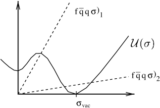
Figure 6: Illustration of the scalar field and quark-scalar-field contributions to the total energy for two choices of the valence quark, scalar density.

In Fig. 6 we see that the lowest energy state is when $q=0$, which is the non-perturbative vacuum with no valence quarks.

$\left.f\bar{q}q\right)_{1}\Rightarrow\sigma\approx 0$ which means that when the scalar, valence quark density is high the perturbative vacuum is restored.

$\left.f\bar{q}q\right)_{2}\Rightarrow\sigma\approx\sigma_{\rm vac}$ which means that when the quark field is small the non-perturbative vacuum is restored.

Figure 7: Formation of a non-topological soliton as a self-consistent combination of localised valence quark density and a “hole” in the non-perturbative vacuum field configuration.

The results of this model are as follows

• The quarks dig a self-consistent “hole” in the scalar field.

• Asymptotically quarks have effective mass for $f\sigma_{\rm vac}$ ($+m$) (where $m$ is the perturbative QCD mass).

• Quarks are only “confined” in the sense that if, for example, $\kappa\sim(1-\frac{\sigma}{\sigma_{\rm vac}})^{n}$ then $\kappa\rightarrow 0$ outside the soliton. Hence the total colour electric energy is infinite, unless $\sum_{i}\lambda_{i}^{a}=0$ — that is, it is a colourless state. This is shown by using the same argument as for a charge in a dia-electric cavity.

7 Colour Dielectric Model

Another interesting model is the Colour Dielectric Model[8, 9, 10].This model gives us an effective description of the long-distance effects in QCD. Once again, we can formulate a Lagrangian to allow the investigation of the theory:

$${\cal L}=i\bar{\psi}\!\!\not\!\partial\psi-\frac{m}{\chi}\bar{\psi}\psi-U(\chi)+\frac{1}{2}{\sigma_{\rm V}}^{2}\left(\partial_{\mu}\chi\right)^{2}-\kappa(\chi){\rm Tr}(G_{\mu\nu}G^{\mu\nu}).$$ (43)

Here we find that $\sigma_{\rm V}\chi$ is a confining scalar field that mimics the non-perturbative effect of the gluons. Note that when $\chi\rightarrow 1$ (inside the soliton) the second term goes to the usual mass term, $m\bar{\psi}\psi$, while as $\chi\rightarrow 0$ the effective mass of the quark goes to infinity, which certainly implies confinement:

$$\chi\rightarrow 0\hskip 11.38109pt\Longrightarrow\hskip 11.38109pt\frac{m}{\chi}\rightarrow\infty.$$ (44)

In the simplest case, the potential term, $U(\chi)$, may be taken to be quadratic in $\chi$:

$$U(\chi)\approx\frac{1}{2}m_{\rm GB}^{2}{\sigma_{\rm V}}^{2}\chi^{2}$$ (45)

8 MIT Bag Model

The MIT bag model is of a similar vintage to the harmonic oscillator shell model discussed earlier. We shall take some care in explaining it because it is still proving to be extremely valuable in theoretical nuclear physics. In particular, a large number of applications of the quark model of nucleon structure have been developed using the MIT bag. Two that we mention especially are the calculation of nucleon properties in medium (for instance in a neutron star), and the Quark Meson Coupling (QMC) model [11]. As a relativistic model which permits analytic solution, the MIT bag also allows us to examine the role of dynamical chiral symmetry breaking in hadron structure – a topic of great current interest (for example) under the heading chiral perturbation theory.

A model developed by Bogolubov [12] in the late 1960’s was the basis for the development of the MIT bag model. The model was an attempt to phenomenologically describe confined, relativistic quarks in a finite region of space. We can view this model as, for example, an analytically solvable version of the Colour Dielectric model (where here $\chi$ is 0 outside and 1 inside the bag). Bogolubov considered the simplest case: a Dirac particle of mass $m$, moving freely within a spherical volume of radius R, in a scalar potential.

$$V_{S}(r)=-\theta(R-r)m$$ (46)

Inside the potential, the effective mass of the quark is 0, and outside the potential (or bag) it is infinite, thus confining the quark inside the bag.

Much of the structure of this model relies upon the time independent Dirac equation

$$H\psi(\vec{r})=E\psi(\vec{r}),$$ (47)

where the Hamiltonian is

$$H=\vec{\alpha}\cdot\vec{p}+\beta(V_{S}(r)+m).$$ (48)

The eigenstates of the Hamiltonian are classified by finding operators that commute with $H$. One of these operators is

$$\vec{j}=\vec{l}+\frac{\vec{\sigma}_{(4\times 4)}}{2},$$ (49)

with $\vec{\sigma}$ necessarily of the form

$$\vec{\sigma}_{(4\times 4)}=\left(\begin{array}[]{cc}\vec{\sigma}&0\\ 0&\vec{\sigma}\end{array}\right).$$ (50)

The other operator is the relativistic analog of an operator involving both spin and orbital angular momentum:

$$k=\vec{\sigma}\cdot\vec{l}+1.$$ (51)

The relativistic analog is the obvious generalisation

$$K = \gamma^{0}(\vec{\sigma}\cdot\vec{l}+1)=\left(\begin{array}[]{cc}k&0\\ 0&-k\end{array}\right)$$ (54)

$$= \beta(\vec{\sigma}\cdot\vec{l}+1).$$ (55)

So we can construct eigenstates of $\vec{l}+\vec{s}$ thus

$$\left|l\>\frac{1}{2}\>j\>\mu\right>\equiv\left|\chi_{\kappa}^{\mu}\right>,$$ (56)

and hence define

$$K\left|\chi_{\kappa}^{\mu}\right>=-\kappa\left|\chi_{\kappa}^{\mu}\right>.$$ (57)

Using the above definitions, and the identities listed in the Appendix, it can be shown that $H$ does indeed commute with both $j$ and $K$, and that $j$ and $K$ commute with each other, that is

$$\left[H,j\right]=0=\left[H,K\right]=\left[j,K\right].\hskip 28.45274pt\mbox{\boldmath${\rm Ex\,\char 35\relax}9$}$$ (58)

The easiest way to obtain the eigenvalues of $K$ is to square it, and then operate on a wave function $\psi$. So we find:

$$K^{2} = \beta^{2}\left[(\vec{\sigma}\cdot\vec{l})^{2}+2\vec{\sigma}\cdot\vec{l}+1\right]$$ (59)

$$= l^{2}+\vec{\sigma}\cdot\vec{l}+1$$

$$= \vec{j}^{2}+\frac{1}{4},$$

and hence

$$K^{2}\psi = (\vec{j}^{2}+\frac{1}{4})\psi$$ (60)

$$= (j(j+1)+\frac{1}{4})\psi$$

$$= (j+\frac{1}{2})^{2}\psi.$$

We see that the eigenvalues of $K$ are $\kappa=\pm(j+\frac{1}{2})$, and thus

$$\kappa=\left\{\begin{array}[]{ll}l&{\rm for}\;j=l-\frac{1}{2}\\ -l-1&{\rm for}\;j=l+\frac{1}{2}\end{array}\right.$$ (61)

thereby defining both $l$ and $j$ by the one quantum number $\kappa$.

Now, using

$$\vec{\nabla}=\hat{r}\frac{\partial}{\partial r}-i\frac{\hat{r}}{r}\times\vec{l},\hskip 28.45274pt\mbox{\boldmath${\rm Ex\,\char 35\relax}10$}$$ (62)

we can show that

$$\vec{\alpha}\cdot\vec{p}=-i\vec{\alpha}\cdot\hat{r}\frac{\partial}{\partial r}+\frac{i}{r}\vec{\alpha}\cdot\hat{r}\left(\beta\kappa-1\right).$$ (63)

Substituting this back into Eq. (47) and solving we find that $\psi$ has a general solution of the form

$$\psi_{\kappa}^{\mu}=\left[\begin{array}[]{c}g(r)\chi_{\kappa}^{\mu}\\ if(r)\chi_{-\kappa}^{\mu}\end{array}\right],$$ (64)

which satisfies the following coupled, ordinary differential equations

$$\left(E-V_{\rm s}(r)-m\right)g = -\left(\frac{df}{dr}+\frac{f}{r}\right)+\frac{\kappa f}{r},$$

$$\left(E+V_{\rm s}(r)+m\right)f = \left(\frac{dg}{dr}+\frac{g}{r}\right)+\frac{\kappa g}{r}.$$ (65)

For the most elementary case, $\kappa=-1$ (s${}_{\frac{1}{2}}$), these equations simplify to

$$\frac{d^{2}u}{dr^{2}}+(E^{2}-(m+V_{\rm s})^{2})u=0,$$ (66)

where the substitution $u=rg$ has been made. Naturally there is a similar equation for $l$ $(=rf)$. It is left as an exercise for the reader to show that by following the method of confinement, suggested by Bogolubov [12], which involves defining the scalar potential as

$$V_{\rm s}(r)=\left\{\begin{array}[]{rr}{-m}&{\rm for}\;r\leq R\\ 0&{\rm for}\;r>R,\end{array}\right.$$ (67)

it can be show that, requiring $u$ and $l$ continuous at $r=R$ implies

$$\cos(\!ER)+\frac{\sqrt{(1-(E/m)^{2})}}{1+(E/m)}\sin(\!ER)=\frac{\sin(\!ER)}{ER}\left(1-\frac{E}{E+m}\right).$$ (68)

$${\rm Ex\,\char 35\relax}11$$

This gives us a boundary condition for this model. By taking the confining limit ($m\rightarrow\infty$) we get the eigenvalue condition, given by the relationship between the spherical Bessel functions

$$j_{0}(ER)=j_{1}(ER).$$ (69)

The energy levels may be parameterised by the definition

$$E_{n\kappa}=\frac{\Omega_{n\kappa}}{R},$$ (70)

where $n$ is the principle quantum number. We now find that the first two positive roots of the $\kappa=-1$ states are:

$$\Omega_{1-1}=2.04\; \longleftrightarrow \;1\rm{s}_{\frac{1}{2}},$$ (71)

$$\Omega_{2-1}=5.40\; \longleftrightarrow \;2\rm{s}_{\frac{1}{2}},$$ (72)

and further solutions are easily computed.

Thus Eq. (64) can be rewritten as

$$\psi_{n,\kappa}(\vec{r}) \equiv \psi_{n,-1}(\vec{r})$$ (75)

$$= N_{n,-1}\left[\begin{array}[]{c}j_{0}\left(\frac{\Omega r}{R}\right)\\ i\vec{\sigma}\cdot\hat{r}j_{1}\left(\frac{\Omega r}{R}\right)\end{array}\right]\chi^{\mu}_{-1}.$$

Figure 8: Pictorially we can see that $u(r)=l(r)$ at the boundary ($r=R$)

Confinement is achieved in the MIT bag model by requiring that there is no quark current flow through the surface of the bag. The (charge) density for the Dirac equation is given by

$$j^{0} \equiv \rho=\bar{\psi}\gamma^{0}\psi$$ (76)

$$\propto \left[{j_{0}}^{2}\left(\frac{\omega r}{R}\right)+{j_{1}}^{2}\left(\frac{\omega r}{R}\right)\right],$$

so that the charge density is proportional to the baryon number density. We also note that the space components of the current are given by

$$\vec{j}(\vec{r})=\bar{\psi}\vec{\gamma}\psi=\psi^{\dagger}\vec{\alpha}\psi,$$ (77)

so it is found that

$$\hat{r}\cdot\vec{j}(\vec{r}) = \left(j_{0},-i\vec{\sigma}\cdot\hat{r}j_{1}\right)\left(\begin{array}[]{cc}0&\vec{\sigma}\cdot\hat{r}\\ \vec{\sigma}\cdot\hat{r}&0\end{array}\right)\left(\begin{array}[]{c}j_{0}\\ i\vec{\sigma}\cdot\hat{r}j_{1}\end{array}\right)$$ (82)

$$= ij_{0}j_{1}-ij_{0}j_{1}=0.$$ (83)

In particular, at $r=R$, we can see that $\hat{r}\cdot\vec{j}=0$, so there is no flow of quark current through the surface.

As a side issue, the reader might like to note that for a typical hadronic radius, $R\sim 1$ fm, the charge radius for a proton is

$$\left<r^{2}\right>^{1/2}_{\rm ch}=0.82{\rm fm},$$ (84)

and

$$\frac{\Omega}{R}\sim 400{\rm MeV},$$ (85)

which should be compared with the constituent quark mass.

8.0.1 Magnetic moment

We now consider the case of a charged quark in this potential and introduce a constant magnetic field $\vec{B}$ to the system. Naturally we have

$$\vec{A}=\frac{1}{2}\vec{B}\times\vec{r}.\hskip 28.45274pt\mbox{\boldmath${\rm Ex\,\char 35\relax}12$}$$ (86)

The quark current has a magnetic moment $\vec{\mu}$ that satisfies

$$-\vec{\mu}\cdot\vec{B}=-\int dV\vec{j}\cdot\vec{A}.$$

By making a substitution for $\vec{j}$ (Eq. 77), and for $\vec{A}$ (Eq. 86) we have

$$-\vec{\mu}\cdot\vec{B} = -\frac{e}{2}\int dV\left(\psi^{\dagger}\vec{\alpha}\psi\right)\cdot\left(\vec{B}\times\vec{r}\right)$$ (87)

$$= -\frac{e}{2}\int dV\vec{r}\times\left(\psi^{\dagger}\vec{\alpha}\psi\right)\cdot\vec{B}.$$

Noting that both sides involve a dot product with $\vec{B}$ we find

$$\vec{\mu} = \frac{e}{2}\int dV\vec{r}\times\psi^{\dagger}\vec{\alpha}\psi$$ (88)

$$\vdots\hskip 5.69054pt({\rm algebra})$$

$$= \mu_{\rm conf}\vec{\sigma},$$

where

$$\mu_{\rm conf} = \frac{eR}{2\Omega}\cdot\left\{\frac{4\Omega-3}{6(\Omega-1)}\right\}$$ (89)

$$= \frac{e}{2``m_{\rm const}{\char 34\relax}}\left\{0.83\right\},$$ (90)

and as noted earlier, $m_{\rm const}\equiv\Omega/R$ is like a constituent quark mass. One should note that the previous relationship for $\frac{\mu_{p}}{\mu_{n}}(=-\frac{3}{2})$ is preserved.

8.0.2 Axial current

We know that axial current is very important for weak interactions, and that it is calculated by

$${\bf A}^{\mu}=\bar{\psi}\gamma^{\mu}\gamma_{5}\frac{{\mbox{\boldmath$\tau$}}}{2}\psi,$$ (91)

where $\tau$ is the 3 Pauli matrices for isospin and

$$\psi=\left(\begin{array}[]{c}u\\ d\end{array}\right),$$ (92)

where both $u$ and $d$ are a four component spinor.

In the non-relativistic limit $\vec{A}_{i}$ dominates. The gamma matrices give us

$$\gamma^{0}\vec{\gamma}\gamma_{5}=\left(\begin{array}[]{cc}1&0\\ 0&-1\end{array}\right)\left(\begin{array}[]{cc}0&\vec{\sigma}\\ -\vec{\sigma}&0\end{array}\right)\left(\begin{array}[]{cc}0&1\\ 1&0\end{array}\right)=\left(\begin{array}[]{cc}\vec{\sigma}&0\\ 0&\vec{\sigma}\end{array}\right),$$ (93)

and in the non-relativistic situation we have $\psi$ nearly, but not exactly equal to $\left(\begin{array}[]{c}1\\ 0\end{array}\right)$, so

$$\vec{A}_{i}\simeq\vec{\sigma}_{i}\frac{\tau_{i}}{2}$$ (94)

with equality when $\psi=\left(\begin{array}[]{c}1\\ 0\end{array}\right)$ – the index $i$ is an index in isospin.

Another exercise for the reader is to show, for the non-relativistic quark model, using the spin-isospin wave function obtained earlier, that:

$$\frac{\left<p\uparrow\right|\sum_{j=1}^{3}\frac{\sigma_{jz}\tau_{j3}}{2}\left|p\uparrow\right>}{\left<p\uparrow\right|\frac{\sigma_{z}\tau_{3}}{2}\left|p\uparrow\right>}=\frac{5}{3},\hskip 28.45274pt\mbox{\boldmath${\rm Ex\,\char 35\relax}13$}$$ (95)

where the index $j$ labels the quarks, and the denominator involves simply the baryon spin-isospin operators. Thus, with the spin-flavor wave functions we have used and the nucleon axial charge operator, we find that

$$\frac{g_{\rm A}}{g_{\rm V}}=\left(\frac{\left<p\uparrow\right|\vec{{\bf A}}\left|p\uparrow\right>}{\left<p\uparrow\right|\frac{\vec{\sigma}{\mbox{\boldmath$\tau$}}}{2}\left|p\uparrow\right>}\right)=\frac{5}{3}.$$ (96)

However, from the $\beta$-decay of free neutrons we know that it is 1.26!

One suggestion to remedy this problem with $g_{A}$ was that there might be a strong tensor force which would mix a sizeable d-state (L=2) component into the nucleon wavefunction, thus reducing $g_{A}$. Exploration of the deformation of the $\Delta$, through the E2/M1 ratio in the $\Delta\rightarrow N\gamma$ transition has since suggested that this is unlikely to be the correct explanation – the N and $\Delta$ do not appear to have a significant, intrinsic deformation.

On the other hand, for our case the quarks are not non-relativistic:

$$\bar{\psi}\vec{\gamma}\gamma_{5}\frac{\mbox{\boldmath$\tau$}}{2}\psi = \left(j_{0},-i\vec{\sigma}\cdot\hat{r}j_{1}\right)\left(\begin{array}[]{cc}\vec{\sigma}&0\\ 0&\vec{\sigma}\end{array}\right)\left(\begin{array}[]{c}j_{0}\\ i\vec{\sigma}\cdot\hat{r}j_{1}\end{array}\right)$$ (101)

$$= \left[\left\{j_{0}\left(\frac{\Omega r}{R}\right)\right\}^{2}\vec{\sigma}+(\vec{\sigma}\cdot\hat{r})\vec{\sigma}(\vec{\sigma}\cdot\hat{r})\left\{j_{1}\left(\frac{\Omega r}{R}\right)\right\}^{2}\right]\frac{\mbox{\boldmath$\tau$}}{2},$$ (102)

and

$$\int dV\bar{\psi}(\vec{r})\vec{\gamma}\gamma_{5}\frac{\mbox{\boldmath$\tau$}}{2}\psi(\vec{r}) = {\cal N}^{2}\int_{0}^{R}drr^{2}\left[\left\{j_{0}\left(\frac{\Omega r}{R}\right)\right\}^{2}\right.$$

$$\left.-\frac{1}{3}\left\{j_{1}\left(\frac{\Omega r}{R}\right)\right\}^{2}\right]\vec{\sigma}\frac{\mbox{\boldmath$\tau$}}{2},$$

$${\rm Ex\,\char 35\relax}14$$

(For reference ${\cal N}^{2}=\left[\int_{0}^{R}drr^{2}\left({j_{0}}^{2}+{j_{1}}^{2}\right)\right]^{-1})$

$$\stackrel{{\scriptstyle\rm(numerical)}}{{=}}0.65\vec{\sigma}\frac{\mbox{\boldmath$\tau$}}{2}.$$

This implies that

$$\frac{g_{\rm A}^{\rm bag}}{g_{\rm V}} = 0.65\times\frac{5}{3}$$ (104)

$$= 1.09,$$

a result which constitutes nearly a 50% improvement in the error and thus may be considered a major success of relativistic quantum mechanics. However this success is tempered with the knowledge that the quarks were taken to be massless. If we were to give the quarks a “current quark” mass, the lower component would decrease and hence $g_{\rm A}$ increase, so that in the heavy quark limit $g_{\rm A}$ increases to $\frac{5}{3}$.

This model of Bogolubov produces many interesting results, but the value of the bag radius, $R$, is chosen in an ad hoc manner. What is needed is a self-consistent link between the size of the cavity, and what is in it, similar to the soliton models. This self-consistency was supplied by the MIT bag model in a fully covariant way. We specialise to the spherical, static cavity (which is the only case that is easily solved in 3+1 dimensions ).

8.0.3 Lagrangian formulation

In the static cavity approximation the Lagrangian density describing the MIT bag is:

$${\cal L}_{\rm cav}=\left[\bar{q}(i\!\!\not\!\partial-m)q-B\right]\theta_{\rm V}-\frac{1}{2}\bar{q}q\delta_{\rm S},$$ (105)

where the last term results in the quarks being infinitely massive at the surface of the cavity. For the present we have not included the gluons for simplicity. (To include the gluons we must include a term $-\frac{\kappa}{4}{\rm Tr}(G\cdot G)$, with

$$\kappa=\left\{\begin{array}[]{ll}1&\;\mbox{ inside the cavity}\\ 0&\;\mbox{ outside the cavity}\end{array}\right.$$ (106)

and make the substitution $\partial\rightarrow D$.) We have defined:

$$\theta_{\rm V} = \theta(R-r),$$ (107)

$$\delta_{\rm S} = \delta(r-R),$$ (108)

and the Euler-Lagrange equation

$$\frac{\partial{\cal L}}{\partial\bar{q}}-\partial_{\mu}\frac{\partial{\cal L}}{\partial(\partial_{\mu}\bar{q})}=0,$$ (109)

is satisfied. We demand that the action is stationary under the following transformations

$$q \rightarrow q+\delta q,$$

$$\bar{q} \rightarrow \bar{q}+\delta\bar{q},$$

$$R \rightarrow R+\delta R.$$ (110)

The final transformation results in

$$\theta_{\rm V} \rightarrow \theta_{\rm V}+\delta_{\rm S}(\delta R),$$

$$\delta_{\rm S} \rightarrow \delta_{\rm S}-n\cdot\partial\delta_{\rm S},$$ (111)

where $n^{\mu}=(0,\hat{r})$ is defined to be an outward normal.

Exercise 15 for the reader is to show that these transformations lead to the following equations

$$\left.\begin{array}[]{cl}i\!\!\not\!\partial q=mq&r\leq R,\\ &\mbox{Dirac Equation}\\ i\gamma\cdot nq=q&r=R,\\ &\mbox{linear boundary condition (l.b.c.)}\\ B=-\frac{1}{2}n\cdot\partial(\bar{q}q),&r=R,\\ &\mbox{non-linear boundary condition (n.l.b.c.)}\end{array}\right\}\mbox{\boldmath${\rm Ex\,\char 35\relax}15$}$$ (112)

Exercise 16 is to show that the linear boundary condition implies that at $r=R$,

$$n_{\mu}j^{\mu} = +\bar{q}q$$ (113)

$$= -\bar{q}{q}$$

$$= 0,\hskip 28.45274pt\mbox{\boldmath${\rm Ex\,\char 35\relax}16$}$$

As $\bar{q}q$ vanishes at $r=R$, it can be shown that the total energy of three identical quarks is given by

$$E(R)=3\frac{\Omega}{R}+\frac{4\pi}{3}R^{3}B,$$ (114)

where the first term comes from the Dirac equation and the second term can be thought of as the volume energy. We also find the non-linear boundary condition is the same as the Lee soliton, that is

$$\frac{\partial E(R)}{\partial R}=0 \Rightarrow \frac{3\Omega}{R^{2}}=4\pi BR^{2}$$ (115)

$$\Rightarrow R=\left(\frac{3\Omega}{4\pi B}\right)^{1/4}$$

Thus we can choose $B$ once and fix it, and then calculate the size of each of the hadrons since the radius is determined by what energy state the quarks are in. To get a instinctive feeling for this equation one can visualise it as requiring that the pressure from the vacuum is balanced by the energy of the quarks at the surface of the bag.

Since this model, as described, is quite simplistic, possible improvements are easy to imagine and often easy to implement. One of the most important extensions was the inclusion of the zero point and centre of mass corrections

$$E(R)\rightarrow E(R)-\frac{z_{0}}{R}.$$ (116)

Also one gluon exchange may be included by solving Maxwell’s equation in a cavity, subject to the confining boundary conditions. This leads to a hyperfine interaction which has the same dependence on spin and colour as the hyperfine interaction discussed earlier and hence we get the required $N-\Delta$, $\Sigma-\Lambda$ mass splitting, etc.

Given ${\cal L}_{\rm cav}$ we can follow the common procedure used in QCD and look at the symmetries, and hence the conserved currents. Recall Noether’s theorem, that if ${\cal L}(\psi_{i},\partial_{\mu}\phi_{i})$ is invariant (i.e. $\delta{\cal L}=0$) under the transformation

$$\phi_{i}\rightarrow\phi_{i}+f_{i}(\phi_{j})\varepsilon,$$ (117)

where $\varepsilon$ is an infinitesimal constant, then

$$j^{\mu}=\frac{\partial{\cal L}}{\partial(\partial_{\mu}\phi_{i})}f_{i}$$ (118)

is conserved. Thus we have that if ${\cal L}={\cal L}_{\rm symm}+{\cal L}_{\rm break}(\phi_{i})$, then from the Euler-Lagrange equation:

$$\partial_{\mu}j^{\mu}=\frac{\partial{\cal L}_{\rm break}}{\partial\phi_{j}}f_{j}.$$ (119)

We now will look at some of the symmetries in the model.

8.0.4 Example  #5 U(1) invariance

It is easy to show that the Lagrangian density

$${\cal L}_{\rm cav}=\left[i\bar{q}\!\!\not\!\partial q-B\right]\theta_{V}-\frac{1}{2}\bar{q}q\delta_{\rm S},$$ (120)

is invariant under the phase transformations

$$q \rightarrow q+i\varepsilon q,$$

$$\bar{q} \rightarrow \bar{q}-i\varepsilon\bar{q}.$$ (121)

Thus we find that the baryon number current (up to a factor $1/3$):

$$j^{\mu} = \left(i\bar{q}\gamma^{\mu}\right)(-iq)\theta_{\rm V}$$ (122)

$$= \bar{q}\gamma^{\mu}q\theta_{\rm V},$$

is conserved.

8.0.5 Example  #6 – Isospin Current

If we define $q=\left(\begin{array}[]{c}u\\ d\end{array}\right)$, then we find that ${\cal L}_{\rm cav}$ is invariant under

$$q \rightarrow q+i\frac{\mbox{\boldmath$\tau$}\cdot\mbox{\boldmath$\varepsilon$}}{2}q,$$

$$\bar{q} \rightarrow \bar{q}-i\bar{q}\frac{\mbox{\boldmath$\tau$}\cdot\mbox{\boldmath$\varepsilon$}}{2}.$$ (123)

It is left as an exercise for the reader to check that the isospin current is conserved and is given by

$$j^{\mu}=\bar{q}\gamma^{\mu}\frac{\mbox{\boldmath$\tau$}}{2}q\theta_{\rm V}.\hskip 28.45274pt\mbox{\boldmath${\rm Ex\,\char 35\relax}17$}$$ (124)

8.0.6 Example  #7 – Axial Current

For two-flavour, massless, QCD, ${\cal L}$ is invariant under

$$q \rightarrow q-i\frac{\mbox{\boldmath$\tau$}\cdot\mbox{\boldmath$\varepsilon$}}{2}\gamma_{5}q,$$

$$\bar{q} \rightarrow \bar{q}-i\bar{q}\frac{\mbox{\boldmath$\tau$}\cdot\mbox{\boldmath$\varepsilon$}}{2}\gamma_{5},$$ (125)

which are chiral transformations, and there exists a conserved axial current

$$\mbox{\boldmath$A$}^{\mu}=\bar{q}\gamma^{\mu}\gamma_{5}\frac{\mbox{\boldmath$\tau$}}{2}q.$$ (126)

However for ${\cal L}$ the surface term “$-\frac{1}{2}\bar{q}q\delta_{\rm S}$” is not invariant under the chiral transformation, Eq. (125), and therefore

$$\mbox{\boldmath$A$}^{\mu}=\bar{q}\gamma^{\mu}\gamma_{5}\frac{\mbox{\boldmath$\tau$}}{2}q\theta_{\rm V},$$ (127)

satisfies

$$\partial_{\mu}\mbox{\boldmath$A$}^{\mu}=-i\bar{q}\gamma_{5}\frac{\mbox{\boldmath$\tau$}}{2}q\delta_{\rm S},$$ (128)

and we see (as illustrated in Fig. 9) that the confining boundary violates chiral symmetry – i.e. mixes left- and right-handed quarks. This is a major problem since symmetries should always be a crucial guide in constructing models.

Figure 9: Violation of chiral symmetry at the bag surface

But QCD already has a problem. If $\partial_{\mu}\mbox{\boldmath$A$}^{\mu}=0$ then

$$\int_{\mbox{All Space}}dV\partial_{\mu}\mbox{\boldmath$A$}^{\mu}=0,$$ (129)

implies

$$\partial_{0}\left\{\int dV\mbox{\boldmath$A$}^{0}\right\}=-\int dV\vec{\nabla}\cdot\vec{\mbox{\boldmath$A$}}=0,$$ (130)

by the Gauss Theorem. By defining the axial charge as $\mbox{\boldmath$Q$}_{5}=\int dV\mbox{\boldmath$A$}^{0}$ we find that it is a constant of the motion, that is

$$\left[H,\mbox{\boldmath$Q$}_{5}\right]=0.$$ (131)

Thus for all positive parity eigenstates of the Hamiltonian there exists a degenerate, negative parity state, i.e.

$$H\left|N^{+}\right>=m\left|N^{+}\right>\Rightarrow\mbox{\boldmath$Q$}_{5}\left|N^{+}\right> = \left|N^{-}\right>\;{\rm has}$$

$$H\left|N^{-}\right> = m\left|N^{-}\right>.$$ (132)

This is clearly not seen in nature!

The solution comes through the Goldstone Theorem. Either these degenerate, negative parity states exist OR $\mbox{\boldmath$Q$}^{5}\left|0\right>\neq 0$. That is, as a result of spontaneous symmetry breaking, there exists massless, pseudoscalar Goldstone bosons. As the first option is clearly incorrect, in an effective low energy description of QCD, we require a massless “pion” field, $\phi$, in addition to the quarks. so that ${\cal L}_{\rm cav}$ is invariant. Naturally, if we probe this at high momentum transfer the $\pi$ will show its internal $\bar{q}q$ structure. This is the basis of the Cloudy Bag Model [13] discussed in Sec. 9, which has a Lagrangian of the form

$${\cal L}_{\rm CBM}=\left[i\bar{q}\!\!\not\!\partial q-B\right]\theta_{\rm V}-\frac{1}{2}\bar{q}e^{i\mbox{\boldmath$\tau$}\cdot\mbox{\boldmath$\phi$}\gamma_{5}/f}q\delta_{\rm S}+\frac{1}{2}\left(D_{\mu}\mbox{\boldmath$\phi$}\right)^{2},$$ (133)

where

$$D_{\mu}\mbox{\boldmath$\phi$} = \left(\partial_{\mu}\phi\right)\hat{\phi}+f\sin\left(\frac{\phi}{f}\right)\partial_{\mu}\hat{\phi},$$ (134)

$$= \partial_{\mu}\mbox{\boldmath$\phi$}+{\cal O}(\phi^{3}).$$ (135)

and ${\cal L}_{\rm CBM}$ is invariant under

$$q \rightarrow q-i\frac{\mbox{\boldmath$\tau$}\cdot\mbox{\boldmath$\varepsilon$}}{2}\gamma_{5}q,$$

$$\bar{q} \rightarrow \bar{q}-i\bar{q}\frac{\mbox{\boldmath$\tau$}\cdot\mbox{\boldmath$\varepsilon$}}{2}\gamma_{5},$$

$$\phi \rightarrow \mbox{\boldmath$\phi$}+\mbox{\boldmath$\varepsilon$}f+f\left(\mbox{\boldmath$\varepsilon$}\times\hat{\phi}\right)\times\hat{\phi}\left[1-\frac{\phi}{f}\cot(\frac{\phi}{f})\right].$$ (136)

Thus

$$\mbox{\boldmath$A$}^{\mu} = \bar{q}\gamma^{\mu}\gamma_{5}\frac{\mbox{\boldmath$\tau$}}{2}q\theta_{\rm V}+\left[f\hat{\phi}(\partial^{\mu}\phi)+\frac{f^{2}}{2}\partial^{\mu}\hat{\phi}\sin(\frac{2\phi}{f})\right]$$ (137)

$$= \mbox{\boldmath$A$}^{\mu}_{\rm quark}+f\partial^{\mu}\mbox{\boldmath$\phi$}+{\cal O}(\phi^{3}).$$

9 The Cloudy Bag Model (CBM)

The basic premise for this model is that we work perturbatively about MIT bag model solutions. This can be compared to the Skyrme models or the topological soliton models, where the pion field dominates the dynamics. The question remains as to whether they are equivalent. For QCD in 1+1 dimensions this equivalence can be demonstrated, but in 3+1 dimensions the belief is that the equivalence is broken.

The CBM Lagrangian is defined to be

$${\cal L}_{\rm CBM} \cong \left(i\bar{q}\!\!\not\!\partial q-m\bar{q}q-B\right)\theta_{\rm V}-\frac{1}{2}\bar{q}q\delta_{\rm S}-$$ (138)

$$\frac{i}{2f}\bar{q}\gamma_{5}\frac{\mbox{\boldmath$\tau$}}{2}q\cdot\mbox{\boldmath$\phi$}\delta_{\rm S}+\frac{1}{2}\left(\partial_{\mu}\mbox{\boldmath$\phi$}\right)^{2}-\frac{1}{2}m_{\pi}^{2}\mbox{\boldmath$\phi$}^{2},$$

and here the terms involving $m$ use the current quark mass to slightly (partially) break exact chiral symmetry. We also see that chiral symmetry requires (at least) linear coupling of pions to the bag through the $\mbox{\boldmath$\tau$}\cdot\mbox{\boldmath$\phi$}$ term. That is, the CBM Lagrangian reduces to the MIT bag plus a free pion field with interactions between the two dictated by chiral symmetry.

$${\cal L}_{\rm CBM}\cong{\cal L}_{\mbox{MIT Bag}}+{\cal L}_{\rm Free-\pi}+{\cal L}_{\rm int}.$$ (139)

Hence this implies that

$$H = H_{\rm MIT}+H_{\pi}+H_{\rm int}$$ (140)

$$= \sum_{\alpha}\varepsilon_{\alpha}\alpha^{\dagger}\alpha+\sum_{k}\omega_{k}a_{k}^{\dagger}a_{k}+\sum_{\alpha,\beta,k}\left[\beta^{\dagger}\alpha a_{k}v^{\beta\alpha}_{k}+{\rm h.c.}\right],$$ (141)

where ($k=\vec{k},i$) and

$$v^{\beta\alpha}_{\vec{k},i}=\frac{i}{2f}\frac{1}{\sqrt{2\omega_{k}}}\int dV\exp^{-i\vec{k}\cdot\vec{r}}\delta(r-R)\left<\beta\right|\bar{q}(\vec{r})\gamma_{5}\mbox{\boldmath$\tau$}_{i}q(\vec{r})\left|\alpha\right>,$$ (142)

with $\left<\beta\right|$ and $\left|\alpha\right>$ being bag states. We stress that the pion-baryon couplings involve form factors which arise naturally as a consequence of the internal structure of the baryons and which can be calculated using the underlying quark model – be it a bag or something more sophisticated.

Another exercise for the reader is, for $\alpha=\left|N\right>$, and $\beta=\left|N^{\prime}\right>$, using

$$N^{2}_{n,\kappa}\equiv N^{2}_{1,-1}=\frac{\Omega^{3}}{2R^{3}(\Omega-1)\sin^{2}\Omega},$$ (143)

to prove that

$$v_{\vec{k},i}^{N^{\prime}N} = -\left(2\omega_{k}\right)^{-1/2}\frac{i}{2f}\frac{\Omega}{(\Omega-1)}\frac{j_{1}(kR)}{kR}$$ (144)

$${}_{SI}\left<N^{\prime}\right|\sum_{\alpha=1}^{3}\tau_{\alpha i}\vec{\sigma}_{\alpha}\cdot\vec{k}\left|N\right>_{\rm SI}.\hskip 28.45274pt\mbox{\boldmath${\rm Ex\,\char 35\relax}18$}$$

Hence we see that using $g_{\rm A}^{\rm Bag}=\left(\frac{\Omega}{\Omega-1}\right)\frac{5}{9}$, and

$$u(k)\equiv\frac{3j_{1}(kR)}{kR}\;\left(\stackrel{{\scriptstyle k\rightarrow 0}}{{\longrightarrow}}1\right),$$ (145)

it can be shown

$$v_{\vec{k},i}^{N^{\prime}N}=-\frac{i}{(2\omega_{k})^{1/2}}\left(\frac{g_{\rm A}^{\rm Bag}}{2f}\right)u(k)\left<N^{\prime}\right|\tau_{i}\vec{\sigma}\cdot\vec{k}\left|N\right>,$$ (146)

and comparing to the usual $\pi NN$ coupling, we find

$$\frac{g_{\pi NN}}{2m_{N}}=\frac{g_{\rm A}}{2f}.$$ (147)

With a little rearrangement, we find that

$$fg_{\pi NN}=g_{\rm A}m_{N},$$ (148)

which is the Goldberger-Treiman relation.

From this same ${\cal L}$ we can derive various coupling constants and form-factors, for instance, $\Delta N\pi,\Delta\Delta\pi,\Sigma\Lambda\pi,\Sigma\Sigma\pi,\Xi\Xi\pi,$ etc.

9.0.1 Example  #8 The physical/dressed nucleon

We have included some examples that may assist in the understanding of this model here. The physical nucleon, $\left|\tilde{N}\right>$, is the eigenstate of the CBM Hamiltonian with eigenvalue $m_{N}$:

$$H\left|\tilde{N}\right>=m_{\rm N}\left|\tilde{N}\right>.$$ (149)

This should be compared with the eigenstate of the MIT bag piece of the Hamiltonian:

$$H_{\rm MIT}\left|N\right>=m_{\rm N}^{(0)}\left|N\right>,$$

$$H_{\rm MIT}\left|\Delta\right>=m_{\Delta}^{(0)}\left|\Delta\right>,$$

$${\rm e.t.c.}$$ (150)

where the one gluon exchange splittings, which may or may not be equal to the mass splittings of the observed baryons, is included in the $m^{(0)}$ terms. In first order perturbation theory:

$$\left|\tilde{N}\right> = \sqrt{Z}\left\{\left|N\right>+\sum_{\alpha,k}\frac{\left<\alpha\pi_{k}\right|H_{\rm int}\left|N\right>}{m_{\rm N}-w_{k}-m_{\alpha}}\left|\alpha\pi_{k}\right>\right\}$$ (151)

$$\cong \sqrt{Z}\left\{\left|N\right>+\sum_{k}c_{1}(k)\frac{\left|N\pi_{k}\right>}{-\omega_{k}}+\sum_{k}c_{2}(k)\frac{\left|\Delta\pi_{k}\right>}{m_{\rm N}-\-m_{\Delta}-\omega_{k}}\right\}.$$ (152)

The convergence of this perturbative expansion can be proven to be extremely good as long as $R$ is large ($\geq 0.7$fm) – i.e. the form-factor is soft – and as long as we restrict our model space to low-lying bag states (e.g. $N,\Delta[R,\ldots]$) – similar to the $2\hbar\omega$ restriction in the non-relativistic oscillator model.

9.0.2 Example  #9 – Charge distribution of $n$

Suppose we ignore spin-spin effects (small in the bag), then we find that the neutron bag has no charge distribution. On the other hand, the wave function of the physical neutron is:

$$\left|\tilde{n}\right>=\sqrt{z}\left\{\left|n\right>+\sum_{k}c_{1}(k)\left[\left(\frac{2}{3}\right)^{1/2}\left|p\pi_{k}^{-}\right>+\left(\frac{1}{3}\right)^{1/2}\left|n\pi^{0}\right>\right]+\ldots\right\}.$$ (153)

Here we see that $\left|n\right>$ contributes nothing as does $\left|n\pi^{0}\right>$. The coefficients $\frac{2}{3}$ and $\frac{1}{3}$ should be instantly recognizable as the Clebsch-Gordon coefficients for isospin coupling. Since there is only one term ($\left|p\pi^{-}_{k}\right>$) that contributes (at this order) we can now see that the leading order effect in producing a non-zero charge distribution for the neutron is the (proton bag) + (pion cloud) component of the neutron wave function [14].

It is easy to see that, as the bag has a sharp surface, this simple model will produce a zero in the neutron charge density at the bag radius [14]. Detailed calculations of the neutron charge distribution are complicated by the need to project a state of good total momentum and to remove spurious centre of mass motion (which cannot be treated exactly as it was in the oscillator model). Nevertheless, after all the necessary corrections are made this feature persists to quite good accuracy. In Fig. 10, we see the results of a very recent calculation [15], which illustrate the importance of the current measurements of the neutron charge form factor at MIT Bates, TJNAF and Mainz.

Figure 10: Neutron charge density calculated in the CBM for several choices of bag radius. Note that the peak in the negative charge density always occurs very near the chosen value of R.

9.0.3 Example  #10 – Corrections to bag mass

To lowest, non-trivial, order (second order in $H_{\rm int}$) we have

$$m_{N} = m_{N}^{(0)}+\frac{3f_{NN\pi}^{2}}{\pi m_{\pi}^{2}}\int_{0}^{\infty}dk\frac{k^{4}u^{2}(k)}{\omega_{k}(m_{N}-\omega_{K}-E_{N}(k))}$$ (154)

$$+\frac{4}{3}\frac{f_{N\Delta\pi}^{2}}{\pi m_{\pi}^{2}}\int_{0}^{\infty}dk\frac{k^{4}u^{2}(k)}{\omega_{k}(m_{N}-\omega_{K}-E_{\Delta}(k))}.$$

Figure 11: Pion self-energy corrections for the nucleon

Since both these diagrams are attractive there is a sizable correction of -300 to -400 MeV to the total energy.

For comparison we look at the $\Delta-\Delta$ system.

Figure 12: Pion self-energy corrections for the $\Delta$

It can be show that Fig. 11(a) and Fig. 12(b) are equal in magnitude and that Fig. 12(a) is small. So we find that

$${\rm Re}(m_{\Delta}) = m_{\Delta}^{(0)}+\frac{f_{\Delta N\pi}^{2}}{3\pi m_{\pi}^{2}}{\cal P}\left[\int_{0}^{\infty}dk\frac{k^{4}u^{2}(k)}{\omega_{k}(m_{\Delta}-\omega_{k}-E_{N}(k))}\right]$$ (155)

$$+\frac{75}{16}\frac{f_{\Delta\Delta\pi}^{2}}{\pi m_{\pi}^{2}}{\cal P}\left[\int_{0}^{\infty}dk\frac{k^{4}u^{2}(k)}{\omega_{k}(m_{\Delta}-\omega_{k}-E_{\Delta}(k))}\right],$$

where ${\cal P}$ is the Principal value of the integral and in this case results in severe cancellations. The first integral term is represented by Fig. 12(a) and the second integral represents Fig. 12(b). In this case the attraction leads to a downward shift of 200 to 300 MeV!

Hence we can see that 100 to 200 MeV of the $N-\Delta$ splitting comes from the pion self energy, thus we find that the value of $\alpha_{\rm S}$ is even smaller.

9.0.4 Observation  #1

If $\alpha_{\rm S}\sim 0.3$, as this analysis of the N-$\Delta$ splitting suggested, the spin-orbit problem in the baryon spectrum is essentially resolved.

9.0.5 Observation  #2

Q) How can one ever seriously believe “shell model” type studies if effects of channel coupling are so large

A) You can’t! Each resonance should be studied as a coupled channel scattering problem…Until recently this has been seen as involving too much work! So far it has only been taken seriously in a limited number of cases [2, 3] – see also the discussion of Thomas and Miller[16].

10 Conclusion

In this very limited space we have tried to summarise a great deal of physics that is not often taught. It is assumed that students of the strong interaction have somehow “picked up” the information. In this final, brief section we would like to make a few connections between the simple models and ideas presented here and some modern research topics.

In the past few years it has been realized that a hyperfine interaction involving spin and isospin, rather than spin and colour (as for one gluon exchange) offers some phenomenological improvements in fitting the baryon spectrum [17]. The motivation for such an interaction is that there should be some residual short-distance remnant of the long range pion cloud required by chiral symmetry that we presented here using the CBM. Indeed, it has sometimes been argued that one should include only this interaction with no one gluon exchange term.

There is currently great experimental activity and related theoretical interest in exploring the chiral and deconfinement transitions expected at high baryon density. One may ask whether these phase transitions are coincident or even whether they exist at all. Recent work from several different approaches to QCD[18, 19], suggests that they may be coincident, occurring at 3-4 times normal nuclear matter density. Moreover, these calculations provide a rather unexpected motivation for a model of hadron structure like the bag. Below the critical density for the chiral/deconfining phase transition a region of space containing current quarks is unstable and thus at finite, but low baryon density one expects to form colourless bubbles of chirally restored phase – just like the MIT bag. There is still an enormous amount of work to be done to move from this observation to a real understanding of the best way to model the nucleon, but this work has provided important insight.

Chiral perturbation theory is currently enjoying tremendous popularity, with many fascinating examples of experimental interest being explored [20, 21]. However, it has also been realized that the usual formulation using, for example, dimensional regularization presents some problems. In particular, the chiral corrections grow rapidly with the mass of the Goldstone boson, whereas one would physically expect it to be less important. The CBM has exactly the behaviour as chiral perturbation theory as $m_{\pi}\rightarrow 0$, but the corrections to hadron properties actually get smaller as the Goldstone boson mass increases because of the physically motivated momentum cut-off in the model – recall this cut-off is related to the internal quark structure of the hadron. There is a great deal of important work to be done to combine these two approaches to the same underlying physics – e.g. see Ref. [21].

With regard to the chiral structure of the nucleon we must mention the very exciting experimental results from Fermilab in which, for the first time, we have been given a direct view of the asymmetry between $\bar{d}$ and $\bar{u}$ quarks in the nucleon sea [22]. It seems most likely that this asymmetry, which was anticipated on the basis of the CBM [23], is at least in part due to the pion cloud of the nucleon required by chiral symmetry [24].

We cannot finish a review such as this without mentioning the very fundamental questions at the heart of nuclear theory, for which models such as those described here have an important role to play. In particular, we would very much like to understand the role that nucleon substructure plays in understanding the properties of finite nuclei as well as matter at higher density. As just one example, the quark meson coupling model [25, 26], which is based on the MIT bag, offers a completely new saturation mechanism for nuclear matter that seems very natural. It also offers a consistent theoretical framework for calculating the changes in hadron properties (masses, from factors and so on) in a nuclear medium. There is a great deal of experimental interest in these questions and we hope that these notes may be of some assistance in understanding what is being done and perhaps in contributing to it.

Appendix

Dirac Matrices and Spinors

Throughout this paper we have followed the conventions of Bjorken and Drell [27]. The gamma matrices satisfy the following condition :

$$\{\gamma^{\mu},\gamma^{\nu}\}=\gamma^{\mu}\gamma^{\nu}+\gamma^{\nu}\gamma^{\mu}=2g^{\mu\nu}.$$ (156)

Where the $\gamma$ matrices are defined by:

$$\gamma^{0}=\beta,$$ (157)

$$\vec{\gamma}=\beta\vec{\alpha},$$ (158)

$$\gamma_{5}=\gamma^{5} = i\gamma^{0}\gamma^{1}\gamma^{1}\gamma^{3}$$ (159)

$$= -i\gamma_{0}\gamma_{1}\gamma_{2}\gamma_{3},$$

and their values in the Dirac representation are:

$$\gamma^{0}=\left(\begin{array}[]{cc}I&0\\ 0&-I\end{array}\right),$$ (160)

$$\vec{\gamma}=\left(\begin{array}[]{cc}0&\vec{\sigma}\\ -\vec{\sigma}&0\end{array}\right),$$ (161)

$$\gamma_{5}=\left(\begin{array}[]{cc}0&I\\ I&0\end{array}\right).$$ (162)

Obviously $\gamma^{0}$ is hermitian, $\gamma^{i}$ is antihermitian, $\gamma^{2}_{5}=I$, and finally

$$\{\gamma_{5},\gamma^{\mu}\}=0,\hskip 42.67912pt\gamma^{\mu}=\gamma^{0}\gamma^{\mu\dagger}\gamma^{0}.$$ (163)

Selected Solutions for Exercises

Exercise 1

We find the spin-flavour wave function of the $J_{z}=\frac{1}{2},\Delta^{+}$ in the following way. We act with the spin lowering operator on each quark as shown below.

$$S_{-}\left|\Delta^{+},J_{z}=\frac{3}{2}\right> \propto \left(S_{q}\right)_{-}\left|\widetilde{u\uparrow u\uparrow d\uparrow}\right>$$

$$=\frac{1}{\sqrt{9}} \left\{\left|u\downarrow u\uparrow d\uparrow\right>+\left|u\uparrow u\downarrow d\uparrow\right>+\left|u\uparrow u\uparrow d\downarrow\right>+\right.$$

$$\left.\left|u\downarrow d\uparrow d\uparrow\right>+\left|u\uparrow d\downarrow d\uparrow\right>+\left|u\uparrow d\uparrow d\downarrow\right>+\right.$$

$$\left.\left|d\downarrow u\uparrow d\uparrow\right>+\left|d\uparrow u\downarrow d\uparrow\right>+\left|d\uparrow u\uparrow d\downarrow\right>\right\}$$

$$=\frac{1}{3} \left(\left|\widetilde{u\uparrow u\uparrow d\downarrow}\right>+\left|\widetilde{u\uparrow u\downarrow d\uparrow}\right>\right).$$

Exercise 2

We want to find the wave function of

$$\left|p\uparrow\right>=\left|uud,J_{z}=\frac{1}{2}\right>,$$

which is totally symmetric in Spin-Flavour. We now find all totally symmetric combinations of these spin and flavour combinations.

$$\left(u\uparrow u\uparrow d\downarrow\right)_{\rm Symm(Spin-Flav)}=(u\uparrow u\uparrow d\downarrow)+(u\uparrow d\downarrow u\uparrow)$$

$$+(d\downarrow u\uparrow u\uparrow)$$

and

$$\left(u\uparrow u\downarrow d\uparrow\right)_{\rm Symm(Spin-Flav)} = (u\uparrow u\downarrow d\uparrow)+(u\downarrow u\uparrow d\uparrow)$$

$$(u\uparrow d\uparrow u\downarrow)+(u\downarrow d\uparrow u\uparrow)$$

$$(d\uparrow u\uparrow u\downarrow)+(d\uparrow u\downarrow u\uparrow)$$

We now antisymmeterise with respect to, say, spin ($\uparrow\downarrow$), and we get

$$\left|p\uparrow\right>=\frac{1}{\sqrt{18}}\left(2\left|\widetilde{u\uparrow u\uparrow d\downarrow}\right>-\left|\widetilde{u\uparrow u\downarrow d\uparrow}\right>\right)$$

where $18=2^{2}\times 3+(-1)^{2}\times 6$ (the factors 3 and 6 indicate the number of terms in the kets respectively). Alternatively, we can simply write down the normalized combination of $\left|\widetilde{u\uparrow u\uparrow d\downarrow}\right>$ and $\left|\widetilde{u\uparrow u\downarrow d\uparrow}\right>$ orthogonal to the $\Delta^{+},J_{z}=\frac{1}{2}$ state.

Exercise 3

We shall just present the solutions here, as the reader should be able to obtain these results alone by now.

$$\left|\Sigma^{0}\uparrow\right> = \frac{1}{\sqrt{18}}\left|2(u\uparrow d\uparrow s\downarrow)_{\rm S}-(u\uparrow d\downarrow s\uparrow)_{\rm S}-(u\downarrow d\uparrow s\uparrow)_{\rm S}\right>$$

$$= \frac{1}{\sqrt{18}}\left(2\left|\widetilde{u\uparrow d\uparrow s\downarrow}\right>-\left|\widetilde{u\uparrow d\downarrow s\uparrow}\right>-\left|\widetilde{u\downarrow d\uparrow s\uparrow}\right>\right)$$

$$\left|\Lambda\uparrow\right> = \frac{1}{\sqrt{6}}\left(\left|\widetilde{u\uparrow u\downarrow s\uparrow}\right>-\left|\widetilde{u\downarrow d\uparrow s\uparrow}\right>\right)$$

Exercise 4

We know that

$$\sum_{i=1}^{3}\frac{\mu_{iz}}{2}=\mu_{0}\left\{\frac{2}{3}(\vec{S}_{u})_{z}-\frac{1}{3}(\vec{S}_{d})_{z}-\frac{1}{3}(\vec{S}_{s})_{z}\right\}.$$

So we find

$$\left<p\uparrow\right|\sum_{i}\frac{\mu_{iz}}{2}\left|p\uparrow\right> = \frac{1}{18}\mu_{0}\left<2(u\uparrow u\uparrow d\downarrow)_{\rm S}-(u\uparrow u\downarrow d\uparrow)_{\rm S}\right|\frac{2}{3}(\vec{S}_{u})_{z}$$

$$-\frac{1}{3}(\vec{S}_{d})_{z}-\frac{1}{3}(\vec{S}_{s})_{z}\left|2(u\uparrow u\uparrow d\downarrow)_{\rm S}-(u\uparrow u\downarrow d\uparrow)_{\rm S}\right>$$

$$= \frac{\mu_{0}}{18}\left\{4\left<(u\uparrow u\uparrow d\downarrow)_{\rm S}\right|\sum_{i}\mu_{iz}\left|(u\uparrow u\uparrow d\downarrow)_{\rm S}\right>\right.$$

$$\left.-\left<(u\uparrow u\downarrow d\uparrow)_{\rm S}\right|\sum_{i}\mu_{iz}\left|(u\uparrow u\downarrow d\uparrow)_{\rm S}\right>\right\}.$$

Therefore we find that

$$\left<p\uparrow\right|\sum_{i}\frac{\mu_{iz}}{2}\left|p\uparrow\right>=\frac{\mu_{0}}{18}\left\{4\cdot(\frac{2}{3})\cdot 1\cdot 3\right. + 4\cdot(-\frac{1}{3})\cdot(-\frac{1}{2})\cdot 3$$

$$1\cdot(\frac{2}{3})\cdot 0\cdot 6 + \left.1\cdot(-\frac{1}{3})\cdot(\frac{1}{2})\cdot 6\right\},$$

where the factors in each of the terms of the sum are the factor multiplying the ket, the factor multiplying the spin operator, the sum of the spins of the relevant particle, and the number of terms in the ket, respectively. This simplifies to

$$\mu_{p}\equiv\left<p\uparrow\right|\sum_{i}\mu_{iz}\left|p\uparrow\right>=\mu_{0}$$

Similarly we find that the wavefunction of the spin-up neutron is given by

$$\left|n\uparrow\right>\propto I_{-}\left|p\uparrow\right>$$

Therefore we find that $\mu_{n}=\frac{-2\mu_{0}}{3}$, and hence $\frac{\mu_{p}}{\mu_{n}}=-\frac{3}{2}$.

Exercise 5

Beginning with the fact that

$$\left(\vec{\lambda}_{1}+\vec{\lambda}_{2}+\vec{\lambda}_{3}\right)^{2}\left|N\right>=0.$$

We fully expand the term that is squared. We then use the fact that the particles are indistinguishable. Thus we note that, for instance $\vec{\lambda}_{1}\cdot\vec{\lambda}_{2}\equiv\vec{\lambda}_{1}\cdot\vec{\lambda}_{3}$, so we find

$$3\vec{\lambda}^{2}+3\vec{\lambda}_{1}\cdot\vec{\lambda}_{2}=0,$$

or rearranging we get that

$$\vec{\lambda}_{1}\cdot\vec{\lambda}_{2}=-\vec{\lambda}^{2}.$$

Now, we use the hint that is given

$$\sum_{a}\left(\lambda_{a}\right)^{2}=\frac{16}{3}\equiv\vec{\lambda}^{2},$$

(the sum of the index $a$ is a sum from 1 to 8 – due to the fact that we are working in SU(3)). Substituting back be get

$$\left<\vec{\lambda}_{1}\cdot\vec{\lambda}_{2}\right>_{\rm Baryons} = \frac{1}{2}\left<\vec{\lambda}_{1}\cdot\vec{\lambda}_{2}\right>_{\rm Mesons}$$

$$= \frac{1}{2}\left<\vec{\lambda}^{2}\right>$$

$$= \frac{1}{2}\left(-\frac{16}{3}\right)=-\frac{8}{3},$$

as required.

Exercise 9

The requirement is to show that $[H,\vec{j}]=0=[H,K]=[\vec{j},K]$. Since the working is similar in each case we shall only present a result for the last commutator. We have that

$$[\vec{j},K]\propto\left[\vec{l}+\frac{\vec{\sigma}}{2},\vec{\sigma}\cdot\vec{l}\right],$$

where the proportionality comes from the fact that K is actually multiplied by $\gamma_{0}$. Thus we find

$$[\vec{j},K] \propto \left[\vec{l},\vec{\sigma}\cdot\vec{l}\right]+\frac{1}{2}\left[\vec{\sigma},\vec{\sigma}\cdot\vec{l}\right]$$

$$= \sigma_{j}[l_{i},l_{j}]+\frac{1}{2}[\sigma_{i},\sigma_{j}]l_{j}$$

$$= \sigma_{j}i\varepsilon_{ijk}l_{k}+\frac{1}{2}2i\varepsilon_{ijk}\sigma_{k}l_{j}$$

$$= i\varepsilon_{ijk}(\sigma_{j}l_{k}-\sigma_{j}l_{k})$$

$$= 0,$$

as required.

Exercise 11

To show that $u$ and $l$ are continuous at $r=R$ we need to find solutions for them at $r\leq R$ and $r>R$ and then match at the boundary. For the case of $r\leq R$, Eq. (68) simplifies to

$$u^{\prime\prime}+E^{2}u=0$$

Solving this for $u$ we find that $u=A\sin(Er)$. For $r>R$ we have

$$u^{\prime\prime}+(E^{2}-m^{2})u=0$$

with the general solution $u=\alpha\exp^{\sqrt{E^{2}-m^{2}}r}+\beta\exp^{-\sqrt{E^{2}-m^{2}}r}$. Requiring that that $u$ is finite as the value of r increases (i.e. $u<\infty$ as $r\rightarrow\infty$) we find this general answer simplifies to $u=\beta\exp^{-\sqrt{E^{2}-m^{2}}r}$.

We now require that these solutions match at the boundary ($r=R$). Thus we have

$$u(r=R) = A\sin(ER)$$

$$= \beta\exp^{-\sqrt{E^{2}-m^{2}}R},$$

so we see the solution has the form

$$u=A\sin(ER)\exp^{-\sqrt{E^{2}-m^{2}}(r-R)}$$

Now we require that $f(r)$ is continuous at $r=R$. In the simple case we are examining ($\kappa=-1$) we see $f$ is given by

$$f=(E+(m+V_{\rm S}))^{-1}\frac{dg}{dr}$$

Again, using the substitution $g=\frac{u}{r}$ we have that

$$\frac{dg}{dr}=\frac{1}{r}\left(\frac{du}{dr}-\frac{u}{r}\right).$$

Substituting our two solutions for $u$ at the point $r=R$ we get

$$\frac{1}{E}\left(E\cos(ER)-\frac{\sin(ER)}{R}\right)=\frac{1}{E+m}\left(-\sqrt{m^{2}-E^{2}}\sin(ER)-\frac{\sin(ER)}{R}\right)$$

Rearranging, we find what we sought to find

$$\cos(ER)+\frac{\sqrt{1-(E/m)^{2}}}{1+(E/m)}\sin(ER)=\frac{\sin(ER)}{ER}\left(1-\frac{E}{E+m}\right).$$

References

References

- [1] P. A. M. Guichon, “A nonstatic bag model for the roper resonances,” Phys. Lett. 164B (1985) 361.
- [2] B. C. Pearce and I. R. Afnan, “The renormalized pi n n coupling constant and the p wave phase shifts in the cloudy bag model,” Phys. Rev. C34 (1986) 991.
- [3] C. Schutz, J. Haidenbauer, J. Speth, and J. W. Durso, “Extended coupled channels model for pi n scattering and the structure of n*(1440) and n*(1535),” Phys. Rev. C57 (1998) 1464.
- [4] N. Isgur and G. Karl, “P wave baryons in the quark model,” Phys. Rev. D18 (1978) 4187.
- [5] L. Motyka and K. Zalewski, “Spin effects in heavy quarkonia,” Acta Phys. Polon. B29 (1998) 1437, hep-ph/9803436.
- [6] T. D. Lee, “Particle physics and introduction to field theory,”.
- [7] R. Friedberg and T. D. Lee, “Qcd and the soliton model of hadrons,” Phys. Rev. D18 (1978) 2623.
- [8] H. J. Pirner, G. Chanfray, and O. Nachtmann, “A color dielectric model for the nucleus,” Phys. Lett. 147B (1984) 249.
- [9] H. B. Nielsen and A. Patkos, “Effective dielectric theory from qcd,” Nucl. Phys. B195 (1982) 137.
- [10] L. R. Dodd, A. G. Williams, and A. W. Thomas, “Numerical study of a confining color dielectric soliton model,” Phys. Rev. D35 (1987) 1040.
- [11] A. W. Thomas, “Chiral symmetry and the bag model: A new starting point for nuclear physics,” Adv. Nucl. Phys. 13 (1984) 1–137.
- [12] P. N. Bogolubov, “On a model of quasiindependent quarks,” Annales Poincare Phys. Theor. 8 (1968) 163–190.
- [13] S. Théberge, A. W. Thomas, and G. A. Miller, “The cloudy bag model 1: the (3,3) resoanance,” Phys. Rev. D22 (1980) 2838.
- [14] S. Théberge, G. A. Miller, and A. W. Thomas Can. J. Phys. 60 (1982) 59.
- [15] D. H. Lu, A. W. Thomas, and A. G. Williams, “Electromagnetic form-factors of the nucleon in an improved quark model,” Phys. Rev. C57 (1998) 2628, nucl-th/9706019.
- [16] A. W. Thomas and G. A. Miller, “Comment on quark - meson coupling model for baryon wave functions and properties,” Phys. Rev. D43 (1991) 288–290.
- [17] L. Y. Glozman and D. O. Riska, “The spectrum of the nucleons and the strange hyperons and chiral dynamics,” Phys. Rept. 268 (1996) 263–303, hep-ph/9505422.
- [18] M. Alford, K. Rajagopal, and F. Wilczek, “Qcd at finite baryon density: Nucleon droplets and color superconductivity,” Phys. Lett. B422 (1998) 247, hep-ph/9711395.
- [19] A. Bender, G. I. Poulis, C. D. Roberts, S. Schmidt, and A. W. Thomas, “Deconfinement at finite chemical potential,” Phys. Lett. B431 (1998) 263, nucl-th/9710069.
- [20] V. Bernard, N. Kaiser, and U.-G. Meissner, “Chiral dynamics in nucleons and nuclei,” Int. J. Mod. Phys. E4 (1995) 193–346, hep-ph/9501384.
- [21] J. F. Donoghue and B. R. Holstein, “Improving the convergence of su(3) baryon chiral perturbation theory,” hep-ph/9803312.
- [22] FNAL E866/NuSea Collaboration, E. A. Hawker et. al., “Measurement of the light anti-quark flavor asymmetry in the nucleon sea,” Phys. Rev. Lett. 80 (1998) 3715, hep-ex/9803011.
- [23] A. W. Thomas, “A limit on the pionic component of the nucleon through su(3) flavor breaking in the sea,” Phys. Lett. 126B (1983) 97.
- [24] W. Melnitchouk, J. Speth, and A. W. Thomas, “Dynamics of light anti-quarks in the proton,” hep-ph/9806255.
- [25] P. A. M. Guichon, “A possible quark mechanism for the saturation of nuclear matter,” Phys. Lett. 200B (1988) 235.
- [26] P. A. M. Guichon, K. Saito, E. Rodionov, and A. W. Thomas, “The role of nucleon structure in finite nuclei,” Nucl. Phys. A601 (1996) 349–379, nucl-th/9509034.
- [27] J. D. Bjorken and S. D. Drell, “Relativistic quantum field theory.,”.
- [28] F. E. Close, “An introduction to quarks and partons,”.
- [29] E. Leader and E. Predazzi, “An introduction to gauge theories and modern particle physics. vol. 1: Electroweak interactions, the new particles and the parton model,”.
- [30] E. Leader and E. Predazzi, “An introduction to gauge theories and modern particle physics. vol. 2: Cp violation, qcd and hard processes,”.
- [31] T. Muta, “Foundations of quantum chromodynamics: An introduction to perturbative methods in gauge theories,”.
- [32] A. J. Buras, “Asymptotic freedom in deep inelastic processes in the leading order and beyond,” Rev. Mod. Phys. 52 (1980) 199.
- [33] I. J. R. Aitchison and A. J. G. Hey, “Gauge theories in particle physics: A practical introduction,”.
- [34] F. Mandl and G. Shaw, “Quantum field theory,”.
- [35] R. F. Alvarez-Estrada, F. Fernandez, J. L. Sanchez-Gomez, and V. Vento, “Models of hadron structure based on quantum chromodynamics,”.
- [36] N. Isgur and G. Karl, “Positive parity excited baryons in a quark model with hyperfine interactions,” Phys. Rev. D19 (1979) 2653.