Collective modes and current-algebraic sum rules in nuclear medium

Abstract

In-medium sum rules following from the chiral charge algebra of QCD are reviewed, and new sum rules are derived. The new sum rules relate the $I^{G}(J^{PC})=1^{-}(0^{++})$ excitations (quantum numbers of $a_{0}(980)$) to the scalar and isovector densities, and are nontrivial for the isospin-asymmetric medium. We present an extensive illustration of the sum rules with help of quark matter in the Nambu-Jona–Lasinio model. Collective excitations different from the usual meson branches (spin-isospin sound modes) are shown to contribute significantly to the sum rules and to play a crucial role in the limit of vanishing current quark masses.

INP 1798/PH

and

PACS: 25.75.Dw, 21.65.+f, 14.40.-n

1 Introduction

Over the past years intense efforts have been made to better understand the properties of nuclear systems under extreme conditions [1, 2]. It is commonly accepted that basic properties of hadrons undergo severe modifications in nuclear medium [3, 4, 5, 6, 7, 8, 9, 10]We expect that at sufficiently large densities chiral symmetry is restored. Moreover, we know that already at nuclear saturation density we should find strong medium effects. For instance the quark condensate $\langle\overline{q}q\rangle$ is estimated to drop to about 70% of its vacuum value at the nuclear saturation density, as follows from the model-independent prediction of Refs. [11, 12]. The change in this basic scale of strong interactions, as well as other matter-induced effects, undoubtedly lead to severe modifications of in-medium hadron properties, whose excitation energies, widths, coupling constants, size parameters, etc. undergo changes. The experimental evidence for these effects can be found in studies of mesonic atoms, or in the measurements of dilepton spectra in heavy–ion collisions in the Ceres [13] and Helios [14] experiments at CERN. Much more accurate data on hot and dense matter will be provided by the Hades experiment, and by RHIC in the near future. It is therefore an important task to better understand and describe theoretically mesonic excitations in dense and hot systems.

Recent years have brought new interesting ideas and developments in this field. The incomplete list, relevant for the subject of this paper, contains the possibility of S-wave kaon condensation in nuclear matter [15, 16, 17, 18], and the application of chiral effective Lagrangians and models [18, 19, 20, 21, 22, 23, 24, 25, 26] to nuclear systems. General model-independent predictions for excitations with quantum numbers of the pion, based on chiral charge algebra, were made in Refs. [18, 27, 28, 29, 30]. Our present work summarizes and further extends the results presented there.

The purpose of this paper is twofold: In the first part we review the previously-derived current-algebraic sum rules for pionic excitations in nuclear medium (the generalization of the Gell-Mann–Oakes–Renner relation [18, 27], the sum rule of Ref. [28]), as well as derive new sum rules concerning the excitations with quantum numbers of the $\delta$ (or $a_{0})$ meson ($I^{G}(J^{PC})=1^{-}(0^{++})$) (Sec. 2). We discuss formal predictions following from these sum rules (Sec. 3). Particular attention is drawn to nuclear matter with isospin asymmetry, since this is the case where nontrivial conclusions can be drawn for the behavior of mesonic excitations in the limit of vanishing current quark masses. We discuss the appearance of very soft modes in this limit. In the pion channel there exists a positive-charge mode (for medium of negative isospin density) whose excitation energy scales in the chiral limit as the current quark mass itself, and the the square root of it, as is the case of the vacuum. In the $\delta$ channel there exists a positive-charge mode (for medium of negative isospin density) whose excitation energy scales as the difference of the current masses of the $u$ and $d$ quarks. These modes are shown to completely saturate the sum rules in the limit of vanishing current quark masses.

In the second part of the paper (Sec. 4-8) we present an extensive illustration of the general results with help of quark matter in the Nambu-Jona–Lasinio model [31]. Although quark matter is not a realistic approximation to nuclear matter (except, perhaps, at very large densities), the model is good for the present purpose. The reason is that the Nambu-Jona-Lasinio model is consistent with chiral symmetry and complies to chiral charge algebra relations leading to the sum rules. We show that the results of the model are highly nontrivial: collective states appear in isospin-asymmetric medium (spin-isospin sound modes) and these states are necessary to saturate the sum rules. For certain choice of model parameters, these sound modes become the very soft modes in the limit of vanishing current quark masses, and they completely saturate the sum rules. Finally, we remark that the Nambu–Jona-Lasinio model is interesting in its own, and that much of the expectations concerning the behavior of mesons in medium have been based on calculations carried out in this model [18, 19, 20, 21, 22, 23, 24, 25, 26, 32].

2 Current-algebraic sum rules

In this section we present a set of sum rules that are going to be explored in this paper. The method follows Refs. [28, 30]. The sum rules follow from the $SU(2)\otimes SU(2)$ chiral charge algebra [33, 34] of QCD and involve no extra assumptions, therefore are very general. In the context of effective chiral models such relations were derived in Refs. [18]. In this section we also derive the corresponding relations involving the vector current, i.e. involving the excitations with quantum numbers of the $\delta$ (or $a_{0}(975)$) meson, with $I^{G}(J^{PC})=1^{-}(0^{++})$. For the simplicity of notation the derivation is made for two flavors, generically denoted by $u$ and $d$. The cases involving strangeness ($K$ and $K_{0}^{*}$ excitations) can be obtained from the results below by replacing $u$ or $d$ by $s$.

2.1 Operator identities

Consider the charges corresponding to vector and axial vector rotations, defined in the usual way as $Q^{a}=\int d^{3}xJ_{0}^{a}$ and $Q_{5}^{a}=\int d^{3}xJ_{5,0}^{a}$, with the appropriate currents defined as $J_{\mu}^{a}=\overline{\psi}\gamma_{\mu}\frac{\tau^{a}}{2}\psi$ and $J_{5,\mu}^{a}=\overline{\psi}\gamma_{\mu}\gamma_{5}\frac{\tau^{a}}{2}\psi$. The charges satisfy the $SU(2)\otimes SU(2)$ chiral charge algebra:

$$[Q^{a},Q^{b}]=i\epsilon^{abc}Q^{c},\;\qquad[Q_{5}^{a},Q_{5}^{b}]=i\epsilon^{abc}Q^{c}.$$ (1)

The density of the QCD Hamiltonian is denoted as ${\cal H}_{{\rm QCD}}$. We need explicitly the mass term, ${\cal H}_{{\rm mass}}=\overline{\psi}{\cal M}\psi$, where the current mass matrix is ${\cal M}={\rm diag}(m_{u},m_{d})$. The canonical anticommutation rules for the quark operators, $\{\psi_{\alpha}(\vec{x},t),\psi_{\beta}^{\dagger}(\vec{y},t)\}=\delta^{3}(\vec{x}-\vec{y})\delta_{\alpha\beta}$, and the explicit form of ${\cal H}_{{\rm mass}}$ result in the following operator identities:

$$[Q^{a},[Q^{b},{\cal H}_{{\rm QCD}}(0)]] = \overline{\psi}(0)[\tau^{a}/2,[\tau^{b}/2,{\cal M}]]\psi(0),$$ (2)

$$[Q_{5}^{a},[Q_{5}^{b},{\cal H}_{{\rm QCD}}(0)]] = \overline{\psi}(0)\{\tau^{a}/2,\{\tau^{b}/2,{\cal M}\}\}\psi(0).$$ (3)

Rewriting these relations for the neutral and charged channels (with $\tau^{\pm}=\left(\tau^{1}\pm i\tau^{2}\right)/\sqrt{2}$), we obtain the following operator identities:

$$[Q_{5}^{0},[Q_{5}^{0},{\cal H}_{{\rm QCD}}(0)]] = m_{u}\overline{u}u(0)+m_{d}\overline{d}d(0),$$ (4)

$$[Q_{5}^{-},[Q_{5}^{+},{\cal H}_{{\rm QCD}}(0)]] = \frac{1}{2}(m_{u}+m_{d})\left(\overline{u}u(0)+\overline{d}d(0)\right),$$ (5)

$$[Q^{0},[Q^{0},{\cal H}_{{\rm QCD}}(0)]] = 0,$$ (6)

$$[Q^{-},[Q^{+},{\cal H}_{{\rm QCD}}(0)]] = \frac{1}{2}(m_{u}-m_{d})\left(\overline{u}u(0)-\overline{d}d(0)\right).$$ (7)

Relation (6) is trivial, since the third component of isospin is a good symmetry even when $m_{u}\neq m_{d}$. Relation (7) is nontrivial only if $m_{u}\neq m_{d}$.

2.2 Gell-Mann–Oakes–Renner relations in medium

In Appendix A we present a detailed derivation of sum rules from the above operator identities, and the reader is referred there for the details. The sum rules are obtained by the usual technique: Identities (4–5, 7) are sandwiched by a state $|C\rangle$, given below. Then, a complete set of intermediate states is inserted in the LHS of the identities.

The state $|C\rangle$ is chosen to be a uniform, translationally–invariant state describing nuclear matter. It has fixed baryon number density, $\rho_{B}$, and isospin density, $\rho_{I=1}$. We choose to work in the rest frame of nuclear matter. Let us explain the notation used below: states $|j^{a}\rangle$, where $a$ labels isospin, denote all states that can be reached from the state $|C\rangle$ by the action of the appropriate current. For instance, in the case of the $J_{5,0}^{0}$ operator, the states $|j^{0}\rangle$ have quantum numbers of the neutral pion, and include all possible modes excited “on top” of nuclear matter: the vacuum pion branch, collective modes, 1p-1h, 2p-2h, etc., excitations of the Fermi sea, etc. As shown in Appendix A, the sum rules involve intermediate states with momentum $0$ in the nuclear matter rest frame. The quantity $E_{j^{a}}$ denotes the excitation energy of the state $|j^{a}\rangle$ (in the rest frame of nuclear matter). The symbol $\sum_{j^{a}}$ includes the sum over discrete states, as well as the integration over continuum states.

Relations (4-5) result in sum rules which are in-medium generalizations of the Gell-Mann–Oakes–Renner (GMOR) relations [35]:

$$-m_{u}\langle\overline{u}u\rangle_{C}-m_{d}\langle\overline{d}d\rangle_{C} = \sum_{j^{0}}\left|\langle j^{0}|J_{5,0}^{0}(0)|C\rangle\right|^{2},$$ (8)

$$-(m_{u}+m_{d})\langle\overline{u}u+\overline{d}d\rangle_{C} = \sum_{j^{-}}{\rm sgn}(E_{j^{-}})\left|\langle j^{-}|J_{5,0}^{-}(0)|C\rangle\right|^{2}$$ (9)

$$+\sum_{j^{+}}{\rm sgn}(E_{j^{+}})\left|\langle j^{+}|J_{5,0}^{+}(0)|C\rangle\right|^{2}.$$

Indeed, in the case of the vacuum, $|C\rangle=|{\rm vac}\rangle$, we can single out the one-pion contribution in the RHS of Eq. (8-9). Let us denote this state (with 3-momentum 0) as $|\pi^{a}\rangle$. For example, in the case of (8) we then find $\langle\pi^{0}|J_{5,0}^{0}(0)|{\rm vac}\rangle=m_{\pi^{0}}F_{\pi^{0}}$, where $m_{\pi^{0}}$ and $F_{\pi^{0}}$ are the neutral pion mass and decay constant. Therefore, we can write

$$-m_{u}\langle\overline{u}u\rangle_{{\rm vac}}-m_{d}\langle\overline{d}d\rangle_{{\rm vac}}=m_{\pi^{0}}^{2}F_{\pi^{0}}^{2}+\sum_{j^{0}\neq\pi}\left|\langle j^{0}|J_{5,0}^{0}(0)|C\rangle\right|^{2}=m_{\pi^{0}}^{2}F_{\pi^{0}}^{2}+{\cal O}(m^{2}).$$ (10)

The symbol $\sum_{j^{0}\neq\pi}$ denotes the sum over all contributions other than the one-pion-state, e.g. three pions, $\rho+\pi$, etc. As is well known, such contributions are chirally suppressed [36]. They are also infinite, hence require renormalization. Note, however, that since no extra divergencies are introduced by nuclear matter, the vacuum-subtracted sum rules (8-9) are well-defined:

$$-m_{u}\left(\langle\overline{u}u\rangle_{C}-\langle\overline{u}u\rangle_{{\rm vac}}\right)-m_{d}\left(\langle\overline{d}d\rangle_{C}-\langle\overline{d}d\rangle_{{\rm vac}}\right)$$ (11)

$$= \sum_{j^{0}}\left|\langle j^{0}|J_{5,0}^{0}(0)|C\rangle\right|^{2}-\sum_{j^{0}}\left|\langle j^{0}|J_{5,0}^{0}(0)|{\rm vac}\rangle\right|^{2},$$

and similarly for the sum rule (9).

2.3 Additional sum rules

Repeating the steps of the previous section on Eq. (7) we arrive at the sum rule

$$-(m_{u}-m_{d})\langle\overline{u}u-\overline{d}d\rangle_{C}-{\rm vac}$$ (12)

$$= \sum_{j^{-}}{\rm sgn}(E_{j^{-}})\left|\langle j^{-}|J_{0}^{-}(0)|C\rangle\right|^{2}+\sum_{j^{+}}{\rm sgn}(E_{j^{+}})\left|\langle j^{+}|J_{0}^{+}(0)|C\rangle\right|^{2}-{\rm vac},$$

where ${\rm vac}$ means the vacuum subtraction as in Eq. (11). Here the intermediate states have quantum numbers of the $\delta$ meson, ($I^{G}(J^{PC})=1^{-}(0^{++})$).

Subsequent sum rules are obtained from Eqs. (1). The derivation repeats the steps of App. A. We obtain two sum rules involving the isovector density, $\rho_{I=1}=\frac{1}{2}\langle u^{\dagger}u-d^{\dagger}d\rangle_{C}$:

$$\langle u^{\dagger}u-d^{\dagger}d\rangle_{C} = \sum_{j^{-}}\frac{1}{|E_{j^{-}}|}\left|\langle j^{-}|J_{5,0}^{-}(0)|C\rangle\right|^{2}-\sum_{j^{+}}\frac{1}{|E_{j^{+}}|}\left|\langle j^{+}|J_{5,0}^{+}(0)|C\rangle\right|^{2},$$ (13)

$$\langle u^{\dagger}u-d^{\dagger}d\rangle_{C} = \sum_{j^{-}}\frac{1}{|E_{j^{-}}|}\left|\langle j^{-}|J_{0}^{-}(0)|C\rangle\right|^{2}-\sum_{j^{+}}\frac{1}{|E_{j^{+}}|}\left|\langle j^{+}|J_{0}^{+}(0)|C\rangle\right|^{2}.$$ (14)

Sum rules (13) and (14) involve excitations with the quantum numbers of $\pi$ and $\delta$, respectively. These sum rules require no vacuum subtraction, since the left-hand sides involve the matrix element of the conserved vector-isovector current ( $\rho_{I=1}=\langle C|J_{0}^{0}(0)|C\rangle$). If the state $|C\rangle$ is isosymmetric, i.e. $\rho_{I=1}=0$, then the above relations are trivial and just reflect the isospin symmetry of the excitation spectrum.

3 Formal results from the sum rules

For the discussion of this section it is convenient to rewrite the sum rules using the identities

$$E_{j^{a}}\langle j^{a}|J_{5,0}^{a}(0)|C\rangle = \langle j^{a}|\left[H_{{\rm QCD}},J_{5,0}^{a}(0)\right]|C\rangle=\langle j^{a}|\overline{\psi}(0)i\gamma_{5}\left\{\tau^{a}/2,{\cal M}\right\}\psi(0)|C\rangle,$$

$$E_{j^{a}}\langle j^{a}|J_{0}^{a}(0)|C\rangle = \langle j^{a}|\left[H_{{\rm QCD}},J_{0}^{a}(0)\right]|C\rangle=\langle j^{a}|\overline{\psi}(0)\left[\tau^{a}/2,{\cal M}\right]\psi(0)|C\rangle.$$ (15)

Then Eq. (8) becomes

$$-m_{u}\langle\overline{u}u\rangle_{C}-m_{d}\langle\overline{d}d\rangle_{C}-{\rm vac}=\sum_{j^{0}}\frac{1}{E_{j^{0}}^{2}}\left|\langle j^{0}|\left(m_{u}\overline{u}i\gamma_{5}u-m_{d}\overline{d}i\gamma_{5}d\right)|C\rangle\right|^{2}-{\rm vac},$$ (16)

where $j^{0}$ labels all excitations with the quantum numbers of $\pi^{0}$, Eqs. (9,13) give

$$-\langle\overline{u}u+\overline{d}d\rangle_{C}-{\rm vac}$$

$$= \sum_{j^{-}}\frac{m_{u}+m_{d}}{2|E_{j^{-}}|E_{j^{-}}}\left|\langle j^{-}|\overline{d}i\gamma_{5}u|C\rangle\right|^{2}+\sum_{j^{+}}\frac{m_{u}+m_{d}}{2|E_{j^{+}}|E_{j+}}\left|\langle j^{+}|\overline{u}i\gamma_{5}d|C\rangle\right|^{2}-{\rm vac},$$

$$2\rho_{I=1} = \sum_{j^{-}}\frac{\left(m_{u}+m_{d}\right)^{2}}{2|E_{j^{-}}|^{3}}\left|\langle j^{-}|\overline{d}i\gamma_{5}u|C\rangle\right|^{2}-\sum_{j^{+}}\frac{\left(m_{u}+m_{d}\right)^{2}}{2|E_{j^{+}}|^{3}}\left|\langle j^{+}|\overline{u}i\gamma_{5}d|C\rangle\right|^{2},$$ (18)

where $j^{\pm}$ label all excitations with the quantum numbers of $\pi^{\pm},$ and finally Eqs. (12,14) give

$$-\langle\overline{u}u-\overline{d}d\rangle_{C}-{\rm vac}$$

$$= \sum_{j^{-}}\frac{m_{u}-m_{d}}{2|E_{j^{-}}|E_{j^{-}}}\left|\langle j^{-}|\overline{d}u|C\rangle\right|^{2}+\sum_{j^{+}}\frac{m_{u}-m_{d}}{2|E_{j^{+}}|E_{j+}}\left|\langle j^{+}|\overline{u}d|C\rangle\right|^{2}-{\rm vac},$$

$$2\rho_{I=1} = \sum_{j^{-}}\frac{\left(m_{u}-m_{d}\right)^{2}}{2|E_{j^{-}}|^{3}}\left|\langle j^{-}|\overline{d}u|C\rangle\right|^{2}-\sum_{j^{+}}\frac{\left(m_{u}-m_{d}\right)^{2}}{2|E_{j^{+}}|^{3}}\left|\langle j^{+}|\overline{u}d|C\rangle\right|^{2},$$ (20)

where $j^{\pm}$ label all excitations with the quantum numbers of $\delta^{\pm}$.

We stress that the above sum rules are valid for all values of current quark masses, i.e. not necessarily in the chiral ($m_{u}+m_{d}\rightarrow 0$) or isovector ($m_{u}-m_{d}\rightarrow 0$) limits, and hold for all densities $\rho_{B}$ and $\rho_{I=1}$.

3.1 Chiral limit at finite density in isospin-symmetric medium

Now we are going to explore several formal predictions following from Eqs. (16,3,3). The method has been discussed in detail in Refs. [28, 30]. First, we analyze the case when the state $|C\rangle$ carries no isovector density, such as the vacuum or symmetric nuclear matter. To simplify notation we take the strict isovector limit $m_{u}=m_{d}=\overline{m}$. In this case of exact isospin symmetry of the Hamiltionian, as well as of the state $|C\rangle$, the excitation spectrum is invariant under isospin rotations, and clearly $E_{j^{0}}=E_{j^{+}}=E_{j^{-}}$. Also, $\langle\overline{u}u\rangle_{C}=\langle\overline{d}d\rangle_{C}=\langle\overline{q}q\rangle_{C}$. Sum rule (16) becomes

$$-2\langle\overline{q}q\rangle_{C}-{\rm vac}=\sum_{j^{0}}\frac{\overline{m}}{E_{j^{0}}^{2}}\left|\langle j^{0}|\left(\overline{u}i\gamma_{5}u-\overline{d}i\gamma_{5}d\right)|C\rangle\right|^{2}-{\rm vac.}$$ (21)

As long as the chiral symmetry is broken, $\langle\overline{q}q\rangle_{C}$ is non-zero in the chiral limit $\overline{m}\rightarrow 0$. As already mentioned, the vacuum subtraction terms are of order $\overline{m}$, thus are chirally small. Therefore, to match the chiral dimensions on both sides of Eq. (21), there must exist a state, denoted as $\pi^{0}$, for which $\frac{\overline{m}}{E_{\pi^{0}}^{2}}\left|\langle\pi^{0}|\left(\overline{u}i\gamma_{5}u-\overline{d}i\gamma_{5}d\right)|C\rangle\right|^{2}\sim 1$. Since the matrix element $\langle\pi^{0}|\left(\overline{u}i\gamma_{5}u-\overline{d}i\gamma_{5}d\right)|C\rangle$ is finite in the chiral limit, then it follows that $E_{\pi^{0}}\sim\sqrt{\overline{m}}$. Thus, we obtain the same chiral scaling as in the vacuum, where in the chiral limit we have $m_{\pi}=\sqrt{2\overline{m}\langle\overline{q}q\rangle_{0}}/F_{\pi}\sim\sqrt{\overline{m}}$. By isospin symmetry we have

$$E_{\pi^{0}}=E_{\pi-}=E_{\pi+}\sim\sqrt{\overline{m}}.$$ (22)

Note that this result is true for any baryon density.

In principle, in the dense medium there could be more than one state contributing to the sum rule (21) in the chiral limit. It is known that many-body effects of the Fermi sea can induce additional branches of excitations, and we could have several states scaling as (22). Whether or not this occurs is a complicated dynamical issue. The formal result states that there exists at least one state scaling as (22) in the chiral limit.

3.2 Chiral limit at finite density in isospin-asymmetric medium

As shown in Ref. [28], in medium with finite isovector density, $\rho_{I=1}\neq 0$, the behavior of charged excitations in the chiral limit is radically different from the isosymmetric case (22). First, an obvious remark is that since the medium state $|C\rangle$ breaks the isospin invariance, the isospin symmetry of excitations is broken. In fact, at low densities [18] one can relate the splitting of $E_{\pi+}$ and $E_{\pi-}$ to the Weinberg-Tomosawa term in the $\pi$-$N$ scattering, and obtain

$$E_{\pi+}-E_{\pi-}=\frac{\rho_{I=1}}{F_{\pi}^{2}}.$$ (23)

In this approach one takes the low-density limit prior to the chiral limit. Eq. (23) shows that for negative $\rho_{I=1}$ at small densities we have $E_{\pi-}>E_{\pi+}$. However, Eq. (23) cannot be used at large densities.

Now, following Ref. [28], we assume that the isospin density is fixed, and employ sum rules (3-18). Without loss of generality we can assume that $\rho_{I=1}<0$, as in the case of neutron stars or large nuclei. Since $\rho_{I=1}$ is an external property of the system, i.e. independent of the chiral parameter, it is treated as large (finite) in the chiral limit. Then, also the isovector chemical potential, $\mu_{I=1}$, defined as the minimum energy needed to lower the isospin by one unit, is finite in the chiral limit. The excitation energies of positive (negative) isospin can now be written as $E_{j^{\pm}}=\mu_{I=1}\pm\delta E_{j^{\pm}}$, with $\delta E_{j^{\pm}}\geq 0$ by definition of the chemical potential. Hence, for the medium with $\rho_{I=1}<0$, or $\mu_{I=1}<0$, only the positive-isospin excitation energies can vanish. The negative-isospin excitation energies cannot vanish, including the case of the chiral limit. Hence we arrive at the result that for $\rho_{I=1}<0$ the negative-charge excitations are chirally large,

$$E_{j-}\sim 1.$$ (24)

Since the matrix elements $\langle j^{a}|\overline{u}i\gamma_{5}d|C\rangle$ are non-singular in the chiral limit, the sum over negative-isospin excitations, $j^{-}$, in Eqs. (3-18) does not contribute as $m_{u}+$ $m_{d}\rightarrow 0$. Therefore in the chiral limit the negative-charge states do not contribute at all to the sum rules (3-18). For the sum rules to hold, there must exist positive-charge states scaling appropriately in the chiral limit [28]. Assuming there is only one such state, labeled $\pi^{+}$, we find that in the chiral limit

$$-\langle\overline{u}u+\overline{d}d\rangle_{C} = \frac{m_{u}+m_{d}}{2|E_{\pi^{+}}|E_{\pi+}}\left|\langle\pi^{+}|\overline{u}i\gamma_{5}d|C\rangle\right|^{2}$$ (25)

$$-2\rho_{I=1} = \frac{\left(m_{u}+m_{d}\right)^{2}}{2|E_{\pi^{+}}|^{3}}\left|\langle\pi^{+}|\overline{u}i\gamma_{5}d|C\rangle\right|^{2}.$$ (26)

Equations (25-26) give immediately

$$E_{\pi+} = \frac{(m_{u}+m_{d})\langle\overline{u}u+\overline{d}d\rangle_{C}}{2\rho_{I=1}}\sim{\cal O}(m_{u}+m_{d}),$$ (27)

$$\left|\langle\pi^{+}|\overline{u}i\gamma_{5}d|C\rangle\right|^{2} = \frac{(m_{u}+m_{d})\left|\langle\overline{u}u+\overline{d}d\rangle_{C}\right|^{3}}{2\rho_{I=1}^{2}}\sim{\cal O}(m_{u}+m_{d}).$$ (28)

This is totally different from the “usual” behavior in the chiral limit, Eq. (22): the excitation energy of the $\pi^{+}$ mode scales as the current quark mass itself, $m_{u}+m_{d}$, and not $\sqrt{m_{u}+m_{d}}$.

The formal case where more than one state contributes to the sum rules (3-18) in the chiral limit has been analyzed in Ref. [28] in the following way: Assume that the excitation energies of one of these modes scales as $E_{\pi+}\sim\left(m_{u}+m_{d}\right)^{\alpha}$, and the corresponding matrix element scales as $\left|\langle\pi^{+}|\overline{u}i\gamma_{5}d|C\rangle\right|\sim\left(m_{u}+m_{d}\right)^{\beta}$. Since the matrix element is not singular in the chiral limit, one has $\beta\geq 0$. The RHS of the sum rule (18) contains, in the chiral limit, only the positive-charge contributions, which are negative-definite. Therefore no cancellations between contributions of various modes can occur in the chiral limit. The requirement of matching chiral powers on both sides of Eq. (18) gives $3\alpha=2+2\beta$, from which we conclude that $\alpha\geq 2/3$. The positive-charge contributions to the RHS of the sum rule (3) may contain both positive and negative terms, since the sign of $E_{j^{+}}$ is not constrained. This means that there can be cancellations of the leading chiral powers of the positive-charge modes contributing to the sum rule in the chiral limit. Matching of the chiral powers on both sides of Eq. (3) yields therefore the inequality $0\geq 1-2\alpha+2\beta$, which means, together with the previously-derived equality $3\alpha=2+2\beta$, that $\alpha\leq 1$. In case of no cancellations $\alpha=1$. Combining the above results one gets [28]

$$2/3\leq\alpha\leq 1.$$ (29)

Note that these inequalities are nontrivial, since in the vacuum the corresponding power is $\alpha=1/2<2/3$.

Carrying a similar analysis for the neutral pionic excitation in isospin-asymmetric medium we find that in the chiral limit it scales the usual way according to Eq. (22), i.e. as in the isosymmetric case. This is clear, since the medium does not break the third component of isospin.

We conclude this section with several comments. Firstly, the behavior of charged pionic modes in the chiral limit is radically different when the medium breaks the isospin symmetry. For $\rho_{I=1}<0$ the negative-charge excitation has finite energy in the chiral limit, Eq. (24), and the positive-charge excitation becomes very soft, with excitation energy scaling as Eq. (27) (if there is a single mode contributing in the chiral limit) or according to Eq. (29) (if there are more modes). Furthermore, as we will show in the model calculation in the following sections, the nature of this soft mode can be quite complicated: it need not be the excitation branch connected to the pion in the vacuum, but the spin-isospin sound mode, resulting from collective effects in the Fermi sea.

3.3 Isovector limit at finite density

Now we pass to the analysis of Eq. (3-20) in the isovector limit $m_{u}-m_{d}\rightarrow 0$. To our knowledge, results of this section are novel. The method is the same as in the previous sections, with the obvious difference that now we compare the powers of $m_{u}-m_{d}$ rather than $m_{u}+m_{d}$ on both sides of the sum rules (3-20).

In isosymmetric medium $\langle\overline{u}u-\overline{d}d\rangle_{C}\sim m_{u}-m_{d}$. Thus, the powers of $m_{u}-m_{d}$ in Eq. (3) are matched with

$$E_{\delta^{a}}\sim{\cal O}(1),\;a=0,+,-.$$ (30)

This result is not surprising: since $\delta$ is not a Goldstone boson, there is no reason for its mass to vanish in the vacuum, or in isosymmetric medium.

In asymmetric medium the situation is different. Since $\rho_{I=1}=\langle u^{\dagger}u-d^{\dagger}d\rangle_{C}$ is large in the isovector limit, i.e. does not vanish when $m_{u}-m_{d}\rightarrow 0$, also $\langle\overline{u}u-\overline{d}d\rangle_{C}$ is large. This is a direct effect of the asymmetry of the Fermi sea, since the Fermi momenta of $u$ and $d$ quarks (or protons and neutrons) are not equal. As a result, the Fermi seas of particles with opposite isospin contribute differently to $\langle\overline{u}u\rangle_{C}$ and $\langle\overline{d}d\rangle_{C}$. An explicit example is provided later on in Eq. (4).

Repeating the steps of Sec. 3.2 we now find that for $\rho_{I=1}<0$ there must exist at least one state $\delta^{+}$ whose excitation energy scales as $m_{u}-m_{d}$ in the isovector limit. If there is only one such state, then we find

$$E_{\delta^{+}} = \frac{(m_{u}-m_{d})\langle\overline{u}u-\overline{d}d\rangle_{C}}{2\rho_{I=1}}\sim{\cal O}(m_{u}-m_{d}),$$ (31)

$$\left|\langle\delta^{+}|\overline{u}d|C\rangle\right|^{2} = \frac{(m_{u}-m_{d})\left|\langle\overline{u}u-\overline{d}d\rangle_{C}\right|^{3}}{2\rho_{I=1}^{2}}\sim{\cal O}(m_{u}-m_{d}),$$ (32)

Equation (31) shows that there is an exact zero mode in the case of the strict isovector limit $m_{u}=m_{d}$. Such collective modes have been known to occur in many-body physics [37, 38, 39]. If more such states exist, then, in analogy to the case of pionic excitations (cf. the discussion above Eq. (29)), we find that the excitation energies of these states scale as $\left(m_{u}-m_{d}\right)^{\alpha}$, with $2/3\leq\alpha\leq 1$. This result is nontrivial, since in the vacuum the corresponding power is $\alpha=0<2/3$.

3.4 Comments

We end the formal part of this paper with several comments. We stress again that the sum rules of Sec. 3 are valid for arbitrary values of the current quark masses, not necessarily in the chiral or isovector limit, and for arbitrary densities. All kinds of intermediate states contribute to the sum rules: quasiparticles (poles), which can come in multiple branches, 2p-2h continuum, etc.

Another remark concerns the sign of the excitation energy of a mode. As already noticed in Refs. [28, 30], the charged excitation may have negative excitation energy. Note, however, that this does not mean that the system is unstable. This is because charged excitations change the isospin of the system. Suppose we request the state $|C\rangle$ to be the ground state of matter with isospin constrained to the value $I_{3}$. A charged excitation in the sum rules involves isospin $I_{3}\pm 1$. Thus, its isospin is outside the constrained value, and even if the energy of the mode is lower than the energy of $|C\rangle$, it does not mean instability of $|C\rangle$. As a corollary, we notice that states of negative excitation energy cannot be the soft modes of Eq. (27) in the chiral limit. We conclude this from Eq. (27). Since the quark condensate is negative, we get (for media with negative isospin density) that $E_{\pi^{+}}>0$.

4 The Nambu–Jona-Lasinio model

In the remaining parts of this paper we are going to illustrate in detail the general results discussed above by a model calculation. We will consider quark matter in the Nambu–Jona-Lasinio model [31]. This model acquired great popularity in recent years as a framework for calculations of meson and baryon properties, also in the nuclear medium [18, 19, 20, 21, 22, 23, 24, 25, 26] described as a Fermi gas of quarks. Although the description of the nuclear medium by a Fermi gas of quarks is certainly not realistic (unless, perhaps, at very high densities where nucleons deconfine), the model is well-suited for our theoretical purpose: it is consistent with the constraints of chiral symmetry. Therefore it complies to the current-algebra relations, and the sum rules of Sec. 3 hold.

The Lagrangian of the $SU(2)\otimes SU(2)$ Nambu–Jona-Lasinio model is

$${\cal L} = \bar{q}({\rm i}\gamma^{\mu}\partial_{\mu}-{\cal M})q+{\frac{G_{\sigma}}{2}}\left((\bar{q}q)^{2}+(\bar{q}{\rm i}\gamma_{5}\tau^{a}q)^{2}\right)+\frac{{G}_{\delta}}{2}\left((\bar{q}\tau^{a}q)^{2}+(\bar{q}{\rm i}\gamma_{5}q)^{2}\right)$$ (33)

$$\ \ \ -{\frac{G_{\rho}}{2}}\left((\bar{q}\gamma_{\mu}\tau^{a}q)^{2}+(\bar{q}\gamma_{5}\gamma_{\mu}\tau^{a}q)^{2}\right)-{\frac{G_{\omega}}{2}}(\bar{q}\gamma_{\mu}q)^{2}\;,$$

where $q$ is the quark field, ${\cal M}$ is the quark mass matrix, and $G$’s denote the coupling constants in various channels. Using the usual technique of the Hartree approximation one arrives at self-consistency equations for the values of the scalar-isoscalar field $S$, the neutral component of the scalar-isovector field $\delta$, the time component of the neutral vector-isovector field $\rho$, and the time component of the vector-isoscalar field $\omega$:

$$S = \frac{m_{u}+m_{d}}{2}-G_{\sigma}\langle\overline{u}u+\bar{d}d\rangle,\;\delta=\frac{m_{u}-m_{d}}{2}-G_{\delta}\langle\overline{u}u-\bar{d}d\rangle,\;$$

$$\rho = 2G_{\rho}\langle u^{+}u-d^{+}d\rangle,\;\omega=G_{\omega}\langle u^{+}u+d^{+}d\rangle.$$ (34)

For the numerical study in the examples below we use the following two parameter sets, fixed by meson properties in the vacuum:

$$G_{\sigma} = 7.55{\rm GeV}^{-2},\;G_{\delta}=5.41{\rm GeV}^{-2},\;G_{\rho}=7.09{\rm GeV}^{-2},\;$$

$$\;\Lambda = 750{\rm MeV},\;m_{u}=2.52{\rm MeV},\;m_{d}=4.52{\rm MeV},$$ (I)

$$G_{\sigma} = 4.35{\rm GeV}^{-2},\;G_{\delta}=3.34{\rm GeV}^{-2},\;G_{\rho}=12.4{\rm GeV}^{-2},\;$$

$$\Lambda = 954{\rm MeV},\;m_{u}=1.03{\rm MeV},\;m_{d}=3.03{\rm MeV}.$$ (II)

The value of $G_{\omega}$ and the $\omega$ field are not relevant, since we will look for excitations carrying no baryon number. Parameter set I has been used in Ref. [40] to fit the mesonic properties: $m_{\pi}$, $F_{\pi}$, $m_{\rho}=765{\rm MeV}$,, and $m_{\eta}=519{\rm MeV}$. This fits four parameters out of original six. The remaining two parameters are chosen in such a way that $S=361{\rm MeV}$, and the current quark masses $m_{d}$ and $m_{u}$ are arbitrarily split by $2{\rm MeV}$. Parameter set II also fits $m_{\pi}$, $F_{\pi}$, $m_{\eta}$ and $S=361{\rm MeV}$, but not $m_{\rho}$. It uses a much larger value for $G_{\rho}$. Such larger values are needed if one wishes to fit the $a_{11}$ $\pi$-$\pi$ scattering length [41]. Following Ref. [40], we regularize the model using the sharp 3-momentum cut-off. Our results do not qualitatively depend on the choice of the regulator, since the constraints of current algebra are satisfied. The 3-momentum cut-off obeys these requirements, in particular it leads to correct Ward identities [18].

The scalar and vector densities of the $u$ and $d$ quarks are equal to

$$\langle\overline{u}u\rangle = 2N_{c}\int\frac{d^{3}k}{(2\pi)^{3}}\frac{M_{u}}{\sqrt{k^{2}+M_{u}^{2}}}\left(\Theta(k_{u}-|k|)-\Theta(\Lambda-|k|)\right),\;$$

$$\;\;\;\langle\overline{d}d\rangle = 2N_{c}\int\frac{d^{3}k}{(2\pi)^{3}}\frac{M_{d}}{\sqrt{k^{2}+M_{d}^{2}}}\left(\Theta(k_{d}-|k|)-\Theta(\Lambda-|k|)\right),\;$$

$$\langle u^{+}u\rangle = 2N_{c}\int\frac{d^{3}k}{(2\pi)^{3}}\Theta(k_{u}-|k|)\;,\quad\langle d^{+}d\rangle=2N_{c}\int\frac{d^{3}k}{(2\pi)^{3}}\Theta(k_{d}-|k|)\;,$$ (35)

where $\Lambda$ is the sharp three-momentum cut-off, and $k_{u}$ and $k_{d}$ are the $u$ and $d$ quark Fermi momenta, and $\Theta$ is the step function. We have introduced scalar self-energies of $u$ and $d$ quarks, given by

$$M_{u}=S+\delta,\qquad M_{d}=S-\delta.$$ (36)

Self-consistency requires that the quark propagators be evaluated with mean-fields (34):

$$S_{u/d}^{-1}=p-\gamma_{0}(\pm\frac{\rho}{2}+\omega)-M_{u/d}+i\varepsilon\,{\rm sgn}(\mu_{u/d}-p_{0})\;,$$ (37)

where $\mu_{u}$ and $\mu_{d}$ are the chemical potentials of the $u$ and $d$ quarks.

5 Mean fields in medium

We introduce the $x$ and $y$ variables,

$$x=\frac{\rho_{B}}{\rho_{0}}=\frac{\rho_{u}+\rho_{d}}{N_{c}\rho_{0}},\quad y=\frac{\rho_{d}}{\rho_{u}+\rho_{d}},$$ (38)

where $\rho_{0}=0.17{\rm fm}^{-3}$ is the nuclear saturation density, $\rho_{B}$ is the baryon number density, and $\rho_{u/d}$ are the quark densities. The variable $y$ measures the isospin asymmetry of the medium. In symmetric medium $y=$ $\frac{1}{2}$, and in pure neutron matter $\rho_{d}=2\rho_{u}$ and $y=\frac{2}{3}$. The isospin density of the system can be written as $\rho_{{\rm I=1}}=\frac{1}{2}(\rho_{u}-\rho_{d})=N_{c}\rho_{0}x(\frac{1}{2}-y)$. In our study we fix the $x$ and $y$ variables, hence we examine properties of quark matter at a given baryon density and isospin asymmetry.

The first task is to find the mean fields by solving Eqs. (34). For the field $\rho$, which couples to the isospin current, we get immediately $\rho=4G_{\rho}\rho_{{\rm I=1}}=4G_{\rho}N_{c}\rho_{0}x(\frac{1}{2}-y)$. The values of $S$ and $\delta$ are determined by solving numerically the first two of equations (34). Results for $M_{u}$, $M_{d}$ and $-\frac{1}{2}\rho$ are displayed in Fig. 1. For isosymmetric matter (top row) $M_{u}$ is practically equal to $M_{d}$, and the small splitting is caused by the current quark mass difference, $m_{d}-m_{u}=2{\rm MeV}$. For $y=\frac{2}{3}$ (middle row) and $x$ in the range $1$ to $4$ we find that $M_{u}$ is greater than $M_{d}$ by $10-20{\rm MeV}$. At maximum asymmetry (bottom row) the $u$ quark is heavier than the $d$ quark by $100-200{\rm MeV}$. There is a simple physical argument why $M_{u}>M_{d}$ at $y$ above $\frac{1}{2}$: the $d$ quarks are more abundant, and it is energetically preferable for the system to make them lighter.

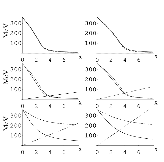
Figure 1: The quark scalar self-energies, $M_{d}$ (solid line) and $M_{u}$ (dashed line), and the vector self-energy of the $d$ quark, $-\frac{1}{2}\rho$ (dotted line) plotted as functions of $x=\rho_{B}/\rho_{0}$ for several values of $y$. The top plots are for $y=1/2$ (isosymmetric matter), the middle plots are for $y=2/3$ (pure neutron matter), and the bottom plots are for $y=1$ (pure $d$-quark matter). The plots on the left (right) are for parameter set I (II).

We note that the field $S$ has a large value of the order ${\cal O}(1)$ if the chiral symmetry is broken. Otherwise it is of the order ${\cal O}(m_{u}+m_{d}).$ The field $\delta$ is large only if $\langle\overline{u}u-\bar{d}d\rangle\sim{\cal O}(1)$, which occurs in isospin-asymmetric medium. In isosymmetric medium $\langle\overline{u}u-\bar{d}d\rangle\sim{\cal O}(m_{u}-m_{d})$, and $\delta$ is small, of the order ${\cal O}(m_{u}-m_{d})$.

6 Meson propagators in medium

As explained in Appendix A, only excitations “at rest” enter the sum rules. Furthermore, we shall only consider the charged meson propagators, since the interesting effects take place for that case.

In the case of no vector-isovector interactions (i.e. $G_{\rho}=0$), the one-quark-loop inverse pion propagator acquires a simple form $1-G_{\sigma}J_{\pi\pi}$, where

$$J_{\pi\pi}(q)=-i{\rm Tr}\int\frac{d^{4}k}{(2\pi)^{4}}\gamma_{5}S_{u}(k+\frac{1}{2}q)\gamma_{5}S_{d}(k-\frac{1}{2}q).$$ (39)

In presence of vector-isovector interactions there is a complication due to the well-known mechanism of mixing of $\pi$ and the longitudinal component of the $A_{1}$ meson. In that case in order to find excitation energies one has to find zeros of the determinant of the inverse $\pi-A_{1}$ propagator matrix, $D_{\pi}$ (see e.g. Ref. [18] for details concerning this problem). The explicit form of the determinant is given in Eq.(51).

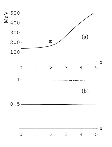
Figure 2: Charged pion in isosymmetric matter ($y=1/2$), parameter set I. (a) Charged pion excitation energy plotted as fuction of $x$. (b) The contribution of the pion poles to sum rule (9): the solid line shows the contribution of $\pi^{+}$ (which equals to the contribution of $\pi^{-}$), the dash-dotted line shows the combined contribution of the two poles.

It is worthwhile to look at the analytic structure of $D_{\pi}$, or equivalently, $J_{\pi\pi}$, in the variable $q_{0}$. The matter state $|C\rangle$ consists of the Fermi seas of $d$ and $u$ quarks, with $k_{d}>k_{u}$, as well as of the Dirac sea occupied down to the cut-off $\Lambda$. A positive-charge Fermi sea excitation moves a quark from the occupied $d$ level to an unoccupied $u$ level. Pauli blocking allows this when

$$\rho+\sqrt{k_{d}^{2}+M_{u}^{2}}-\sqrt{k_{d}^{2}+M_{d}^{2}}<q_{0}<\rho+\sqrt{k_{u}^{2}+M_{u}^{2}}-\sqrt{k_{u}^{2}+M_{d}^{2}}.$$ (40)

Thus, within these boundaries $D_{\pi}(q_{0})$ possesses a cut. The cuts associated with the Dirac sea are within the boundaries:

$$\rho-\sqrt{\Lambda^{2}+M_{u}^{2}}-\sqrt{\Lambda^{2}+M_{d}^{2}} < q_{0}<\rho-\sqrt{k_{d}^{2}+M_{u}^{2}}-\sqrt{k_{d}^{2}+M_{d}^{2}},$$

$$\rho+\sqrt{k_{u}^{2}+M_{u}^{2}}+\sqrt{k_{u}^{2}+M_{d}^{2}} < q_{0}<\rho+\sqrt{\Lambda^{2}+M_{u}^{2}}+\sqrt{\Lambda^{2}+M_{d}^{2}}.$$ (41)

In the delta channel we proceed analogously. We define

$$J_{\delta\delta}(q)=-i{\rm Tr}\int\frac{d^{4}k}{(2\pi)^{4}}S_{u}(k+\frac{1}{2}q)S_{d}(k-\frac{1}{2}q).$$ (42)

For the case $G_{\rho}=0$ the inverse charged $\delta$-meson propagator is $1-G_{\delta}J_{\delta\delta}$. For finite $G_{\rho}$ there occurs mixing between the $\delta$ meson and the longitudinal component of the $\rho$ meson. This mixing is proportional to the mean field $\delta,$ hence it is small, of the order of ${\cal O}(m_{u}-m_{d})$ in isosymmetric medium. The stated behavior can be promptly seen from Eq. (55). If the medium is asymmetric, then the mean field $\delta$ is large, and such is the $\delta-\rho$ mixing. The explicit form of the appropriate determinant, $D_{\delta}$, is given in Eq.(56). The location of the cuts of $D_{\delta}$ is of course the same as in the pion case.

7 Mesons in symmetric matter

Figure 1 shows the results of the numerical calculation of the charged pion excitation in

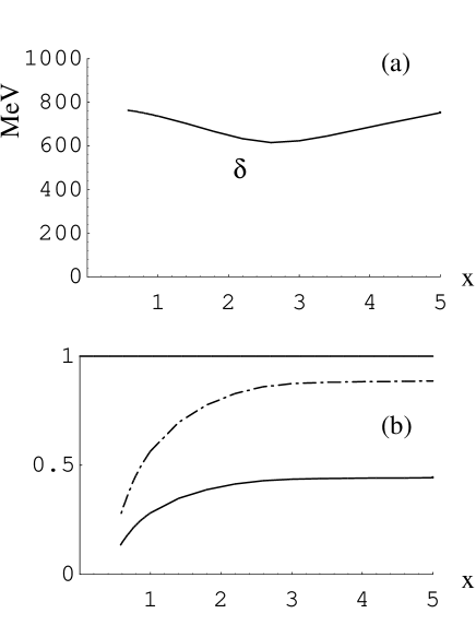
Figure 3: Charged $\delta$ meson in isosymmetric matter ($y=1/2$). (a) The excitation energy plotted as fuction of $x$. (b) The contribution of the $\delta$ poles to sum rule (12): the solid line shows the contribution of $\delta^{+}$ (which equals to the contribution of $\delta^{-}$, the dash-dotted line shows the combined contribution of the two poles.

symmetric matter. In Fig. 2(a) we show the position of the charged pion excitation at rest (usually called the in-medium pion mass) as a function of baryon density. The behavior is the expected one [22], with the pion mass increasing slowly with the baryon density up to about $x\simeq 2$. Above this point chiral symmetry is restored, i.e. $S\sim{\cal O}(m_{u}+m_{d})$, (cf. the upper left Fig. 1) and the pion mass grows more rapidly.

Figure 2(b) shows the anatomy of the in-medium GMOR sum rule (9). We note that up to $x=2$ practically all of the sum rule is saturated by the charged pion poles. At larger $x$ some small ( a few per cent) strength is carried by the cuts (cf. Eqs. (40-41)). We have verified for all other cases shown in this paper that the sum of all pole and cut contributions to the sum rules adds up to 100%. This serves as a check of the numerical calculations.

The case of the charged $\delta$ excitation is displayed in Fig. 3. This excitation emerges as a bound state from the $q\bar{q}$ continuum at $x\simeq 0.6$. Its mass decreases with the baryon density up to $x\simeq 2.5$, and then starts growing (Fig. 3(a)). The contributions to the sum rule (3) are shown in Fig. 3(b). We can see, especially at lower values of $x$, that the pole contribution fall short of saturating the sum rule. Continuum contributions carry about 50% at $x=1$ and about 15% at $x>3$.

8 Mesons in asymmetric matter

In this section we come to the central part of our paper. We will show that in our model the sum

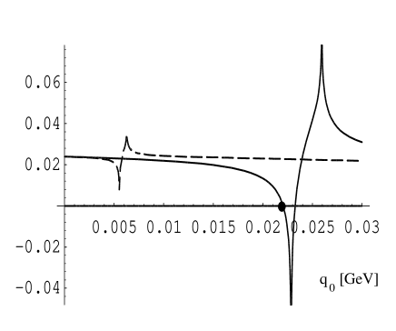
Figure 4: The real part of the pion determinant for $G_{\delta}=4.7{\rm GeV}^{-2}$ (dashed line) and $G_{\delta}=9.4{\rm GeV}^{-2}$ (solid line), plotted as a function of $q^{0}$ for $y=\frac{2}{3}$. Other parameters are: $G_{\sigma}=11.7{\rm GeV}^{-2}$, $\Lambda=619{\rm MeV}$, and $m_{u}=m_{d}=5.7{\rm MeV}$. For large values of $G_{\delta}$ a zero of the inverse pion proparator is induced in the vicinity of the $\overline{d}u$, denoted by a blob. This indicates the presence of the “spin-isospin sound”.

rules from Sec. 3 are, for the case of isospin asymmetric medium, satisfied in a non-trivial way. This involves a collective state, specific for asymmetric medium. As explained e.g. in [42, 43] in the framework of conventional nuclear physics, it is possible for the pion propagator in neutron matter to have an additional pole at very low excitation energies. Such an excitation is known as the spin-isospin sound. We will show that this phenomenon occurs in our model.

The existence of collective modes in our model is related to the presence of the Fermi sea cut (40). Figure 4 shows the real part of the determinant $D_{\pi}$ for $y=\frac{2}{3}$ (pure neutron matter) and two sample parameter choices, plotted as a function of the energy variable $q^{0}$ in the region of the Fermi sea cut. Let us first look at the solid line, corresponding to parameters with a large coupling constant $G_{\delta}$. The presence of the cut manifests itself by the two cusps. The imaginary part of $D_{\pi}$ is nonzero in the region between the two cusps, and vanishes outside. We notice that a zero of $D_{\pi}$ exists in the vicinity of the cut, indicated in the figure by a blob. This zero, at $q^{0}=23{\rm MeV}$, corresponds to the energy of the spin-isospin sound mode. The dashed line, corresponding to lower $G_{\delta}$, also has cusps, but no zero of $D_{\pi}$ exists. This can be understood as follows: the cut region is wider and the function at the cusps acquires higher and lower values as the splitting of the scalar self-energies $M_{u}$ and $M_{d}$ is larger (cf. Eq.(40)). This splitting is proportional to the mean field $\delta$, which increases with $G_{\delta}$, and with asymmetry $y$. Thus we have a critical behavior: above some critical values of asymmetry $y$ and coupling $G_{\delta}$ the spin-isospin mode emerges. We denote it by $\pi_{S}$. In the example shown in Fig. 4 the excitation energy of $\pi_{S}$ is lower than the left boundary of the cut. We find this is the case for small values of the vector-isovector coupling constant $G_{\rho}$. At sufficiently large values of $G_{\rho}$ the collective mode emerges at energies larger than the right boundary of the Fermi cut. In any case, the collective state lies very close to the Fermi sea cut, with excitation energy of the order of $10{\rm MeV}$.

In addition to the collective mode $\pi_{S}$, there exist the usual two charged pion branches, $\pi^{+}$ and $\pi^{-}$, with excitation energies of the order of $m_{\pi}$. These branches connect to the vacuum pion as the baryon density is lowered. Thus, depending on parameters and the value of $y,$ we have, in our model, $2$ or $3$ branches of the charged pion excitations.

For the charged $\delta$ channel the situation is similar: for appropriate parameters and $y>\frac{1}{2}$, a collective mode $\delta_{S}$ appears in addition to the usual $\delta^{+}$ and $\delta^{-}$ modes.

9 Sum rules in asymmetric medium

In this section we show the results of our numerical study. For the case of pionic excitations these results have been already reported in Ref. [30] (for the slightly different parameter cases with $m_{u}=m_{d}$ ).

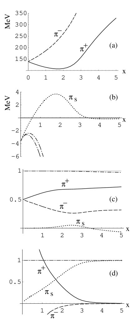
Figure 5: Properties of charged pion excitations for $y=\frac{2}{3}$ and parameter set I, plotted as a function of baryon density. (a) Excitation energies of $\pi^{+}$ and $\pi^{-}$. (b) Excitation energy of $\pi_{S}$ (dotted line) and the boundaries of the Fermi sea cut (dot-dashed line). (c) The relative contribution of $\pi^{+}$, $\pi^{-}$ and $\pi_{S}$ to the in-medium GMOR sum rule (9), and the total contribution from the three poles (dot-dashed line). (d) The relative contribution of $\pi^{+}$, $\pi^{-}$ and $\pi_{S}$ to the sum rule (13). The total contribution from the three poles (dot-dashed line) practically saturates the sum rule.

Figure 5 shows the results for the $\pi$ channel for the parameter set I. Figure 5(a) shows the excitation energies of the usual branches, $\pi^{+}$ and $\pi^{-}$, and Fig. 5 (b) shows the excitation energy of the collective $\pi_{S}$ mode. The dashed-dotted lines show the boundaries of the Fermi-sea cut, (40). The collective mode emerges from the cut at a low value of the baryon density. Its excitation energy is positive for $x$ between $0.6$ and $3.4$, and negative otherwise. In Fig. 5(c) we show the relative contributions from the poles to the in-medium GMOR sum rule, Eq. (9), and the total contribution from the three poles, indicated by the dash-dotted line. The poles practically saturate the sum rule, leaving 1-2% for the cuts at large values of $x$. The contribution of $\pi_{S}$ to the sum rule (9) is of the order of a few per cent. Its sign follows the sign of the excitation energy in Fig. 5(c), as is apparent from Eq. (9). Figure 5(d) shows the relative contribution of the poles to the sum rule (13), and the total pole contribution, indicated by the dash-dotted line. We note that this sum rule is saturated by the pole at the 99.9% level – the cut contributions turn out to be very small. At larger value of $x$ the collective $\pi_{S}$ mode dominates over the other modes, and for $x>3$ it practically saturates the sum rule. We note that the sign of the contributions is associated with the charge of the excitation, as is clear from Eq. (13).

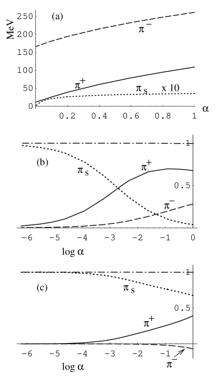
Figure 6: Study of the chiral limit for $x=2$ and $y=\frac{2}{3}$. Convention for line the same as in Fig. 5. (a) Excitation energies, (b) relative contributions to the sum rule (9), and (c) relative contributions to the sum rule (13), plotted functions of $\alpha$, Eq. (43). The spin-isospin sound mode $\pi_{S}$ is the chiral soft mode of Eq. (27). Please, note that $\log\alpha$ means $\ln\alpha$.

Figure 6 shows the result of a formal study of the chiral limit, $m_{u}+m_{d}\rightarrow 0$. For fixed values of $y=\frac{2}{3}$ and $x=2$ we lower the value of

$$\alpha=\frac{m_{u}+m_{d}}{m_{u}^{{\rm phys}}+m_{d}^{{\rm phys}}},$$ (43)

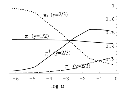
Figure 7: Chiral dimensions of pionic modes plotted as functions of $\log\alpha$, cf. Eq. (43). For the symmetric matter (middle solid line, labeled $y=\frac{1}{2}$, the chiral dimension of the pionic excitations tends to $\frac{1}{2}$ in the chiral limit ($\log\alpha\to-\infty$). For asymmetric matter ($y=\frac{2}{3}$) the chiral dimension of $\pi_{S}$ tends to $1$, and the chiral dimensions of $\pi^{+}$ and $\pi^{-}$ tend to $0$ in the chiral limit. Please, note that $\log\alpha$ means $\ln\alpha$.

where here the superscript ^phys denotes the values from the parameter set (I). Figure 6(a) shows that as the value of $\alpha$ is decreased, the excitation of the modes go down. The excitation energies of $\pi^{+}$ and $\pi^{-}$ modes go to finite values at $\alpha\rightarrow 0$, and the excitation energy of $\pi_{S}$ goes to $0$. Hence $\pi_{S}$ is the chiral soft mode of Eq. (27). Figures 6(b-c)show that in the chiral limit of $\alpha\rightarrow 0$ the $\pi_{S}$ saturates the sum rules (9,13). However, this happens at very low values of $\alpha$, around $\ln\alpha=-4$ or $-5$. Such values of $\alpha$ would correspond to the vacuum value of the pion mass of the order of $15{\rm MeV}$. This indicates that from the point of view of the sum rules we are quite far away from the chiral limit with the physical values of current quark masses, i.e. with $\alpha=1$.

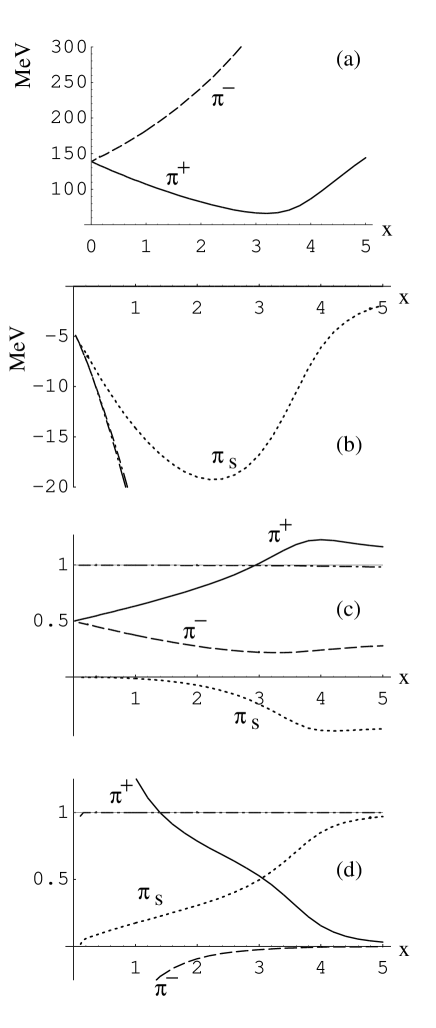
Figure 8: Same as Fig. 5 for parameter set II

In order to better illustrate this point we show in Fig. 7 how the excitation energies of various modes approach the chiral limit. Following Ref. [28] let us introduce ${\rm dim}(X)=\lim_{\overline{m}\to 0}(\log{X}/\log{\overline{m}})$, which we call the chiral dimension of quantity $X$. In the chiral limit a quantity $X$ has some scaling with a power of $m_{u}+m_{d}$. The function ${\rm dim}(X)$ extracts this power (for instance in the vacuum ${\rm dim}(m_{\pi})=1/2$). The dotted line in Fig. 7 shows the chiral dimension of the excitation energy of $\pi_{S}$, which tends to $1$ in the chiral limit, according to Eq. (27). The chiral dimensions of $\pi^{+}$ and $\pi^{-}$ go to $0$ in the chiral limit. The solid line in the middle of the plot is for $\pi^{+}$ or $\pi^{-}$ in symmetric matter, $y=\frac{1}{2}$. In that case, according to Eq. (22), the chiral dimension goes to $\frac{1}{2}$ in the chiral limit.

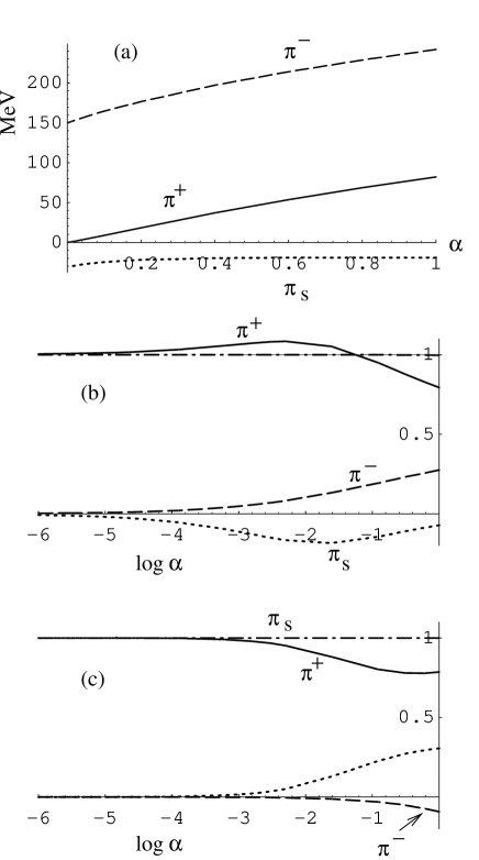
Figure 9: Same as Fig. 6 for parameter set II. The $\pi^{+}$ mode is the chiral soft mode of Eq. (27).

Figures 8-9 show the results for the parameter set II, also for $y=\frac{2}{3}$ as in the case discussed above. The qualitative difference between the present and the former case is that now the spin-isospin sound mode $\pi_{S}$ has negative excitation energy for all values of $x$. Therefore in the chiral limit it is the $\pi^{+}$ mode, not $\pi_{S}$, which becomes the chiral soft mode of Eq. (27) (see Fig. 9 ).

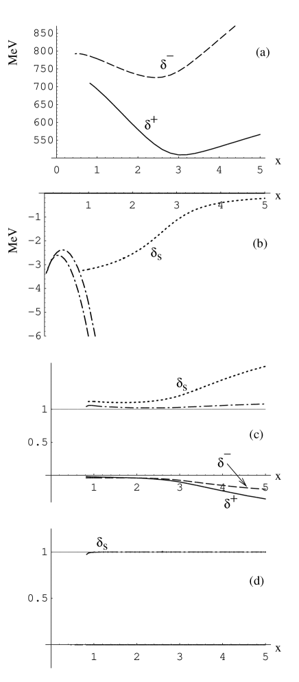
Figure 10: Properties of charged $\delta$ excitations for $y=\frac{2}{3}$ and parameter set I, plotted as a function of baryon density. (a) Excitation energies of $\delta^{+}$ and $\delta^{-}$. (b) Excitation energy of $\delta_{S}$ (dotted line) and the boundaries of the Fermi sea cut (dot-dashed line). (c) The relative contribution of $\delta^{+}$, $\delta^{-}$ and $\delta_{S}$ to the sum rule (12), and the total contribution from the three poles (dot-dashed line). (d) The relative contribution of $\delta^{+}$, $\delta^{-}$ (indistinguishable from $0$) and $\delta_{S}$ to the sum rule (14). The contribution of $\delta_{S}$ saturates the sum rule.

Now we pass to the discussion of the $\delta$ channel, which is done for the parameter set I only, and for $y=\frac{2}{3}$ . Figure 10 (a) shows the excitation energies of the $\delta^{+}$ and $\delta^{-}$ branches. After emerging from the $q\bar{q}$ continuum their energies first decrease until $x\sim 3$, and then start increasing. The collective mode $\delta_{S}$ emerges from the cut at $x\sim 0.75$ (Fig. 11(b)). Its excitation energy is negative and small, less than $3{\rm MeV}$. Figures 10(c-d) show the relative contributions to the sum rules (12) and (14). We note that the $\delta_{S}$ mode plays a major role in sum rule (12), and completely dominates sum rule (14).

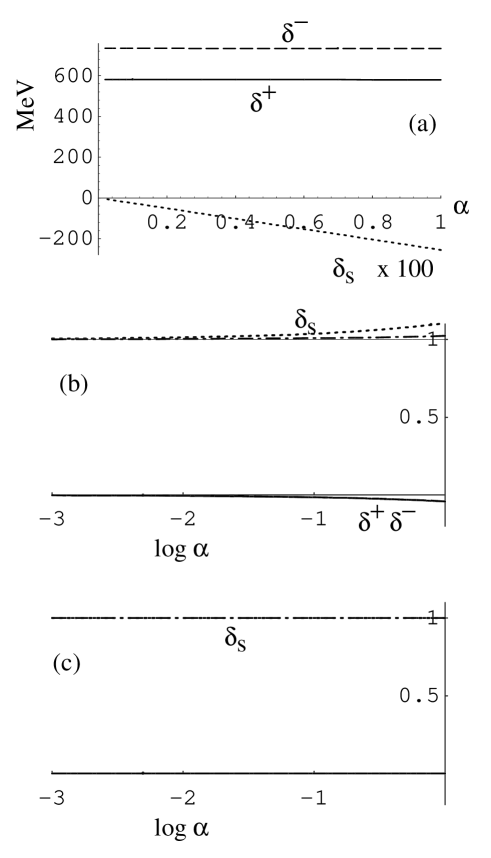
Figure 11: Study of the strict isovector limit for $x=2$ and $y=\frac{2}{3}$. Convention for lines is the same as in Fig. 10. (a) Excitation energies, (b) relative contributions to the sum rule (12), and (c) relative contributions to the sum rule (14), plotted as functions of $\alpha$, Eq. (44). The spin-isospin sound mode $\delta_{S}$ is the isovector soft mode of Eq. (31). It completely satisfies the sum rules in the strict isovector limit. Please, note that $\log\alpha$ means $\ln\alpha$.

Figure 11 shows the isovector limit for the $\delta$ channel. In this case

$$\alpha=\frac{m_{u}-m_{d}}{m_{u}^{{\rm phys}}-m_{d}^{{\rm phys}}}.$$ (44)

We can see that the $\delta_{S}$ mode is the isovector soft mode of Eq. (31). Its excitation energy drops linearly to $0$ as $\alpha$ is decreased (Fig. 11(a)), and the sum rules are completely saturated by the $\delta_{S}$ mode in the isovector limit of $\alpha\rightarrow 0$.

10 Concluding remarks

There are several messages which follow from our calculation. Firstly, we note that in order to satisfy the current-algebraic sum rules it is necessary to include all modes, in particular the spin-isospin sounds. Certainly, a nuclear system is a very complicated object, and even our simple model, treated at the 1p-1h level, has revealed a rich structure of the excitation spectrum. The power of the current-algebraic sum rules relies in the fact that they relate in a non-trivial way the properties of these excitations to the quark condensate and the isospin density.

One may ask the following general questions: How far are we in a nuclear system from the strict chiral limit ( $m_{u}+m_{d}\rightarrow 0$) and the strict isovector limit ( $m_{u}-m_{d}\rightarrow 0$) in the real world, i.e. in a dense nuclear system, and with the physical values of $m_{u}$ and $m_{d}$. The results shown in Figs. 7 and 11 indicate, that in moderately-dense isospin-asymmetric systems we are far away from the chiral limit, and very close to the isovector limit. From Fig. 7 we find that the $\pi_{S}$ mode excitation energy scales linearly with $m_{u}+m_{d}$ starting from $m_{\pi}\simeq\sqrt{e^{-6}}139{\rm MeV}\sim 7{\rm MeV}$, much lower than the physical value. On the other hand, Fig. 10(a) shows that the excitation energy of the $\delta_{S}$ mode scales linearly with $m_{u}-m_{d}$ already at physical value, corresponding to $\alpha=0$.

Another comment is relevant for application of effective chiral Lagrangians to nuclear systems. In this approach one basically assumes that there is one pion quasiparticle in a nuclear medium, albeit with modified properties compared to the vacuum. In our model we find additional branches. Since they contribute largely to the sum rules, they cannot be neglected. In an effective model they should be included as additional degrees of freedom.

The final remark concerns strangeness. Although in this paper we have worked for simplicity with two flavors, extension to three flavors is straightforward. In fact, one can make a simple “translation” of the sum rules of Sec. 3 to the case of any flavor. For example, changing the $d$ (or $u$) quark to $s$ we obtain the case of charged (neutral) kaons. This is simply the replacement of $I$-spin by $U$ or $V$ spins. Note that nuclear matter is asymmetric with respect to $U$ and $V$ spins, therefore kaonic excitations on top of nuclear matter are parallel to the case of charged pionic excitation on top of isospin-asymmetric matter. We note that recently Refs. [44] discussed the kaonic excitations in the Fermi gas of quarks in the Nambu–Jona-Lasinio model.

Appendix A Derivation of sum rules in medium

In this appendix we explain the derivation of sum rules (8-14). Although the technique is very well known, we believe it is worthwhile to remind it in some greater detail in order to point out the differences between the derivation in the vacuum and in a medium. The first step in deriving the sum rules is to sandwich both sides of Eqs. (4-7) by the medium state $|C\rangle$. On the RHS this leads to a “known” quantity involving in-medium condensates $\langle C|\overline{u}u(0)|C\rangle\equiv\langle\overline{u}u\rangle_{C}$ and $\langle\overline{d}d\rangle_{C}$. Next, one inserts a complete set of intermediate states $|\vec{k},j\rangle$ between the current operators on the LHS. These states are eigenstates of the momentum operator, $\widehat{P}$, and of the Hamiltonian $H=\int d^{3}x{\cal H}(\vec{x})$. They can be labeled by additional quantum numbers, e.g. isospin. The medium state is also an eigenstate of $\widehat{P}$ and $H$:

$$\widehat{P}|C\rangle=\vec{p}_{C}|C\rangle,\qquad H|C\rangle={\cal E}_{C}|\vec{k},j\rangle.$$ (45)

For matter of a large volume $V$ the quantities $\vec{p}_{C}$ and ${\cal E}_{C}$ are proportional to $V$. It is convenient to measure the momentum and the energy of intermediate states relative to the state $|C\rangle$,  i.e.

$$\widehat{P}|\vec{k},j\rangle=\left(\vec{k}+\vec{p}_{C}\right)|\vec{k},j\rangle,\qquad H|\vec{k},j\rangle=\left(E_{j}(\vec{k})+E_{C}\right)|\vec{k},j\rangle.$$ (46)

Quantities $\vec{k}$ and $E_{j}(\vec{k})$ form a Lorentz four–vector. Thus the Lorentz-invariant mesure of integration is $\frac{d^{3}k}{|2E_{j}(\vec{k})|}$, and the unit operator can be decomposed as follows [28]:

$$1=\sum_{j}\int\frac{d^{3}k}{\left(2\pi\right)^{3}2|E_{j}(\vec{k})|}|\vec{k},j\rangle\langle\vec{k},j|.$$ (47)

We illustrate the method on Eq. (7). We rewrite the LHS, insert the unit operator (47), express the charges by time-components of currents, shift the coordinates of the currents with the translation operator, and use Eq. (46):

$$[Q^{-},[Q^{+},{\cal H}_{{\rm QCD}}(0)]]=\sum_{j}\int\frac{d^{3}k}{\left(2\pi\right)^{3}2|E_{j}(\vec{k})|}\times$$

$$\left(\langle C|Q^{+}|\vec{k},j\rangle\langle\vec{k},j|[Q^{-},{\cal H}(0)]|C\rangle-\langle C|[Q^{-},{\cal H}(0)]|\vec{k},j\rangle\langle\vec{k},j|Q^{+}|C\rangle\right)=$$

$$= \sum_{j}\int\frac{d^{3}k}{\left(2\pi\right)^{3}2|E_{j}(\vec{k})|}\int d^{3}y\int d^{3}x\times$$

$$\left(\langle C|J_{0}^{+}(\vec{y})|\vec{k},j\rangle\langle\vec{k},j|[J_{0}^{-}(\vec{x}),{\cal H}(0)]|C\rangle-\langle C|[J_{0}^{-}(\vec{y}),{\cal H}(0)]|\vec{k},j\rangle\langle\vec{k},j|J_{0}^{+}(\vec{x})|C\rangle\right)=$$

$$= \sum_{j}\int\frac{d^{3}k}{\left(2\pi\right)^{3}2|E_{j}(\vec{k})|}\int d^{3}y\int d^{3}x\times$$

$$\left(\langle C|e^{i\vec{p}_{C}\cdot\vec{y}}J_{0}^{+}(0)e^{-i\left(\vec{k}+\vec{p}_{C}\right)\cdot\vec{y}}|\vec{k},j\rangle\langle\vec{k},j|e^{i\left(\vec{k}+\vec{p}_{C}\right)\cdot\vec{x}}[J_{0}^{-}(0),{\cal H}(0)]e^{-i\vec{p}_{C}\cdot\vec{x}}|C\rangle\right.$$

$$\left.-\langle C|e^{i\vec{p}_{C}\cdot\vec{y}}[J_{0}^{-}(0),{\cal H}(0)]e^{-i\left(\vec{k}+\vec{p}_{C}\right)\cdot\vec{y}}|\vec{k},j\rangle\langle\vec{k},j|e^{i\left(\vec{k}+\vec{p}_{C}\right)\cdot\vec{x}}J_{0}^{+}(0)e^{-i\vec{p}_{C}\cdot\vec{x}}|C\rangle\right)=$$

$$= \sum_{j}\int\frac{d^{3}k}{2|E_{j}(\vec{k}=0)|}\delta^{3}(\vec{k})\left(\langle C|J_{0}^{+}(0)|\vec{k}=0,j\rangle\langle\vec{k}=0,j|[J_{0}^{-}(0)(0),\int\!\!d^{3}x{\cal H}(0)]|C\rangle\right.$$

$$-\left.\langle C|[J_{0}^{-}(0)(0),\int\!\!d^{3}x{\cal H}(0)]|\vec{k}=0,j\rangle\langle\vec{k}=0,j|J_{0}^{+}(0)|C\rangle\right)=$$

$$= \sum_{j}\frac{1}{2|E_{j}(\vec{k}=0)|}\left(E_{j}(\vec{k}=0)\langle C|J_{0}^{+}(0)|\vec{k}=0,j\rangle\langle\vec{k}=0,j|J_{0}^{-}(0)|C\rangle\right.$$

$$+\left.E_{j}(\vec{k}=0)\langle C|J_{0}^{-}(0)|\vec{k}=0,j\rangle\langle\vec{k}=0,j|J_{0}^{+}(0)|C\rangle\right)=$$

$$= \sum_{j^{+}}\frac{1}{2}{\rm sgn}E_{j^{-}}\left|\langle j^{-}|J_{0}^{-}(0)|C\rangle\right|^{2}+\sum_{j^{+}}\frac{1}{2}{\rm sgn}E_{j^{+}}\left|\langle j^{+}|J_{0}^{+}(0)|C\rangle\right|^{2}.$$

In the last line we have decomposed the sum over indices $j$ into the sum over positive and negative isospin excitations. We have introduced the short-hand notation $|j^{+}\rangle$ and $|j^{-}\rangle$ for such excitations with relative momentum $\vec{k}=0$, and denoted their excitation energies by $E_{j^{+}}$ and $E_{j^{-}}$. This completes the derivation of the sum rule (12). With all other sum rules the steps are exactly the same as described above.

Appendix B Charged meson propagators in medium

The quark bubble for a meson channel is defined as

$$J_{\Gamma\Gamma^{\prime}}(q)=-i{\rm Tr}\int\frac{d^{4}k}{(2\pi)^{4}}\Gamma S_{u}(k+\frac{1}{2}q)\overline{\Gamma}^{\prime}S_{d}(k-\frac{1}{2}q),$$ (48)

where $\overline{\Gamma}=\gamma_{0}\Gamma^{\dagger}\gamma_{0}$ [40]. We use $\Gamma=\gamma_{5}$ in the pion vertex, which allows to get rid of factors of $i$ in Ward identities below. For the considered case of $\vec{q}=0$ the $\pi$-$A_{1}$ mixing involves the time components of the axial propagator, $J_{A_{1}A_{1}}^{00}$, and the mixed propagator, $J_{\pi A_{1}}^{0}$. The determinant of the inverse $\pi$-$A_{1}$ propagator is equal to

$$D_{\pi}(q^{0})=(1-G_{\sigma}J_{\pi\pi}(q^{0}))(1+G_{\rho}J_{A_{1}A_{1}}^{00}(q^{0}))+G_{\sigma}G_{\rho}(J_{\pi A_{1}}^{0}(q^{0}))^{2}.$$ (49)

The signs follow the convention for signs of the coupling constants in Eq. (33). The following Ward identities hold among the bubble functions [40]:

$$(q_{0}-\rho)J_{A_{1}A_{1}}^{00}(q^{0}) = 2SJ_{\pi A_{1}}^{0}(q^{0})+2(u^{\dagger}u-d^{\dagger}d),$$

$$(q_{0}-\rho)J_{\pi A_{1}}^{0}(q^{0}) = 2SJ_{\pi\pi}(q^{0})+2(\bar{u}u+\bar{d}d),$$ (50)

where $\rho$ and $S$ are defined in Eq.(34). These identities follow from the general requirements of chiral symmetry [40]. They can be explicitly verified to hold with our choice of the 3-momentum regulator. Using Eqs. (50,34) we can rewrite Eq. (49) as

$$D_{\pi}(q_{0}) = \frac{q_{0}}{q_{0}-\rho}\left\{\frac{m_{u}+m_{d}}{2S}+\left(\frac{2(m_{u}+m_{d})SG_{\sigma}^{-1}G_{\rho}}{q_{0}(q_{0}-\rho)}-1\right)\times\right.$$ (51)

$$\left.\left[G_{\sigma}J_{\pi\pi}(q_{0})-\frac{2S-(m_{u}+m_{d})}{2S}\right]\right\}\;.$$

This form is convenient, since it involves only one bubble function, $J_{\pi\pi}$, which has the explicit form

$$J_{\pi\pi}(q_{0}) = 4N_{c}\int_{k_{u}}^{\Lambda}\frac{d^{3}k}{(2\pi)^{3}}\frac{(\rho-q_{0})+2\delta M_{u}/\sqrt{k^{2}+M_{u}^{2}}}{(\rho-q_{0})^{2}+2(\rho-q_{0})\sqrt{k^{2}+M_{u}^{2}}+4S\delta}$$

$$+(u\to d,\;\;\rho\to-\rho,\;\;\delta\to-\delta,\;\;q_{0}\to-q_{0})\;.$$ (52)

The zeros of $D_{\pi}(q_{0})$ correspond to poles of the mixed charged $\pi$-$A_{1}$ propagator. The pole contributions to sum rules (9,13) are explicitly given by the expression

$$\!\!\!\!\!\!\!\!\!{\rm sgn}(E_{j^{\pm}})\left|\langle j^{\pm}\mid J_{5,0}^{\pm}\mid C\rangle\right|^{2} = -\left.\frac{m_{u}+m_{d}}{q_{0}-\rho}\frac{\left[SJ_{\pi\pi}(q_{0})-G_{\sigma}^{-1}(S-(m_{u}+m_{d})/2)\right]}{dD_{\pi}(q_{0})/dq_{0}}\right|_{q_{0}=E_{j}^{\pm}}\;.$$

In the $\delta$-$\rho$ channel we obtain, if full analogy to Eq. (49-LABEL:eq:expoleax),

$$D_{\delta}(q^{0})=(1-G_{\delta}J_{\delta\delta}(q^{0}))(1+G_{\rho}J_{\rho\rho}^{00}(q^{0}))+G_{\delta}G_{\rho}(J_{\delta\rho}^{0}(q^{0}))^{2}.$$ (54)

Through the use of Ward identities

$$(q_{0}-\rho)J_{\rho\rho}^{00}(q^{0}) = 2\delta J_{\delta\rho}^{0}(q^{0})+2(u^{\dagger}u-d^{\dagger}d),$$

$$(q_{0}-\rho)J_{\delta\rho}^{0}(q^{0}) = 2\delta J_{\delta\delta}(q^{0})+2(\bar{u}u-\bar{d}d),$$ (55)

where $\rho$ and $\delta$ are defined in Eq.(34), we can rewrite Eq. (54) as

$$D_{\delta}(q_{0}) = \frac{q_{0}}{q_{0}-\rho}\left\{\frac{m_{u}-m_{d}}{2\delta}+\left(\frac{2(m_{u}-m_{d})\delta G_{\delta}^{-1}G_{\rho}}{q_{0}(q_{0}-\rho)}-1\right)\times\right.$$ (56)

$$\left.\left[G_{\delta}J_{\delta\delta}(q_{0})-\frac{2\delta-(m_{u}-m_{d})}{2\delta}\right]\right\}\;,$$

where $J_{\delta\delta}$ is explicitly given by

$$J_{\delta\delta}(q_{0}) = 4N_{c}\int_{k_{u}}^{\Lambda}\frac{d^{3}k}{(2\pi)^{3}}\frac{(\rho-q_{0})+2SM_{u}/\sqrt{k^{2}+M_{u}^{2}}}{(\rho-q_{0})^{2}+2(\rho-q_{0})\sqrt{k^{2}+M_{u}^{2}}+4S\delta}$$

$$+(u\to d,\;\;\rho\to-\rho,\;\;\delta\to-\delta,\;\;q_{0}\to-q_{0})\;.$$ (57)

The zeros of $D_{\delta}(q_{0})$ correspond to poles of the mixed charged $\delta$-$\rho$ propagator. The pole contributions to the sum rules (14) are explicitly obtained from the expression

$$\!\!\!\!\!\!\!\!\!{\rm sgn}(E_{j^{\pm}})\left|\langle j^{\pm}\mid J_{0}^{\pm}\mid C\rangle\right|^{2} = -\left.\frac{m_{u}-m_{d}}{q_{0}-\rho}\frac{\left[\delta J_{\delta\delta}(q_{0})-G_{\delta}^{-1}(\delta-(m_{u}-m_{d})/2)\right]}{dD_{\delta}(q_{0})/dq_{0}}\right|_{q_{0}=E_{j}^{\pm}}\;.$$

References

- [1] For recent developments see Quark Matter 96, proc. 12th Int. Conf. on Ultra-Relativistic Nucleus-Nucleus Collisions, Heidelberg, Germany, 1996, Nucl. Phys. A610, and references therein
- [2] Hadrons in Nuclear Matter, edited by H. Feldmaier and W. Nörenberg (GSI, Darmstadt, 1995), proc. Int. Workshop XXIII on Gross Properties of Nuclei and Nuclear Excitations, Hirschegg, Austria, 1995
- [3] G. E. Brown, Nucl. Phys. A488 (1988) 689c
- [4] W. Weise, Nucl. Phys. A553 (1993) 59C
- [5] C. Adami and G. E. Brown, Phys. Rept. 234 (1993) 1
- [6] B. D. Serot and J. D. Walecka, Advances in Nuclear Physics 16 (1986)
- [7] L. S. Celenza and C. M. Shakin, World Scientific Lecture Notes In Physics, 2 World Scientific (Singapore), 1986,
- [8] G. E. Brown and M. Rho, Phys. Rev. Lett. 66 (1991) 2720
- [9] M. C. Birse, J. Phys. G 20 (1994) 1537
- [10] G. E. Brown and M. Rho, Phys. Rep. 269 (1996) 333
- [11] E. G. Drukarev and E. M. Levin, Nucl. Phys. A511 (1990) 679
- [12] T. D. Cohen, R. J. Furnstahl, and D. K. Griegel, Phys. Rev. C45 (1992) 1881
- [13] CERES Collab., G. Agakichiev et al., Phys. Rev. Lett. 75 (1995)
- [14] HELIOS/3 Collab., M. Masera et al., Nucl. Phys. A590 (1995) 3c
- [15] D. B. Kaplan and A. E. Nelson, Nucl. Phys. A479 (1988) 273c
- [16] H. D. Politzer and M. B. Wise, Phys. Lett. B273 (1991) 156
- [17] G. E. Brown, V. Thorsson, K. Kubodera, and M. Rho, Phys. Lett. B291 (1992) 355
- [18] M. Lutz, A. Steiner, and W. Weise, Nucl. Phys. A 574 (1994) 755
- [19] T. Hatsuda and T. Kunihiro, Progr. Theor. Phys. 74 (1985) 765
- [20] V. Bernard, U.-G. Meissner, and I. Zahed, Phys. Rev. D 36 (1987) 819
- [21] H. Reinhardt and B. V. Dang, J. Phys. G 13 (1987) 1179
- [22] U. Vogl, M. Lutz, S. Klimt, and W. Weise, Nucl. Phys. A516 (1990) 469
- [23] M. Lutz, S. Klimt, and W. Weise, Nucl. Phys. A542 (1992) 521
- [24] M. Jaminon, G. Ripka, and P. Stassart, Nucl. Phys. A504 (1989) 733
- [25] M. C. Ruivo, C. A. de Sousa, B. Hiller, and A. H. Blin, Nucl. Phys. A575 (1994) 460
- [26] S. P. Klevansky, Rev. Mod. Phys. 64 (1992) 642
- [27] T. D. Cohen and W. Broniowski, Phys. Lett. B 342 (1995) 25
- [28] T. D. Cohen and W. Broniowski, Phys. Lett. B 348 (1995) 12
- [29] T. D. Cohen and W. Broniowski, INP Cracow preprint No. 1753/PH (1997), nucl-th/9702027
- [30] W. Broniowski and B. Hiller, Phys. Lett. B 392 (1997) 267
- [31] Y. Nambu and G. Jona-Lasinio, Phys. Rev. 122 (1961) 345
- [32] For a recent review on the model see e.g. J. Bijnens, Phys. Rept. 265 (1996) 369
- [33] S. Adler and R. Dashen, Current Algebras (Benjamin, New York, ADDRESS, 1968)
- [34] V. de Alfaro, S. Fubini, G. Furlan, and C. Rosetti, Currents in Hadron Physics (North-Holland, Amsterdam, ADDRESS, 1973)
- [35] M. Gell-Mann, R. Oakes, and B. Renner, Phys. Rev. 175 (1968) 2195
- [36] J. Gasser and H. Leutwyler, Phys. Lett. 184B (1987) 83; Phys. Lett. 188B (1987) 477; Nucl. Phys. B307 (1988) 763
- [37] A. A. Abrikosov and I. E. Dzialoshinskii, Zh. Eks. Teor. Fiz 35 (1958) 771, [Sov. Phys. JETP 35 (1959) 535]
- [38] E. P. Bashkin, Phys. Lett. A101 (1984) 164
- [39] E. P. Bashkin, C. da Providência, and J. da Providência, Phys. Rev. C 50 (1994) 2800
- [40] S. Klimt, M. Lutz, U. Vogl, and W. Weise, Nucl. Phys. A516 (1990) 429
- [41] V. Bernard, A. H. Blin, B. Hiller, Y. P. Ivanov, A. A. Osipov, and U.-G. Meissner, Ann. Phys. (NY) 249 (1996) 499
- [42] A. B. Migdal, Rev. Mod. Phys. 50 (1978) 107, and references therein
- [43] G. Baym and D. K. Campbell, in in Mesons and Nuclei, edited by M. Rho and D. H. Wilkinson (North Holland, Amsterdam, 1979), p. 1031, and references therein
- [44] C. A. de Sousa and M. C. Ruivo, Nucl. Phys. A625 (1997) 713, Nucl. Phys. A629 (1998) 552c