Abstract: A detailed theoretical investigation of polarization effects in superdeformed nuclei is performed. In the pure harmonic oscillator potential it is shown that when one particle (or hole) with the mass single-particle quadrupole moment $q_{\nu}$ is added to a superdeformed core, the change of the electric quadrupole moment can be parameterized as $q_{eff}=e(bq_{\nu}+a)$, and analytical expressions are derived for the two parameters, $a$ and $b$. Simple numerical expressions for $q_{eff}(q_{\nu})$ are obtained in the more realistic modified oscillator model. It is also shown that quadrupole moments of nuclei with up to 10 particles removed from the superdeformed core of ${}^{152}$Dy can be well described by simply subtracting effective quadrupole moments of the active single-particle states from the quadrupole moment of the core. Tools are given for estimating the quadrupole moment for possible configurations in the superdeformed $A\sim 150$-region.

PACS: 21.60.-n, 21.10.Re, 21.10.Ky

Keywords: Polarization, quadrupole moment, harmonic oscillator, Nilsson-Strutinsky, superdeformation.

1 Introduction

Superdeformed rotational bands were first identified [Twi86] from transition energies only. At an early stage, crude measurements of (electric) quadrupole moments were performed [Ben87] which were an important evidence for the large deformation. Recently, it has become possible to measure relative quadrupole moments with a much higher precision [Sav96, Nis97, Hac98]. Since the total quadrupole moment depends sensitively on the specific orbitals that are occupied, these quadrupole moments have become an important tool to verify configurations of different bands. It is the aim of the present paper to study in detail how the quadrupole moment depends on occupied single-particle states in superdeformed nuclei.

Adding a particle with a single-particle quadrupole moment, $q_{\nu}$, to a core causes a change in deformation due to polarization effects. The size of the deformation change depends on the relative deformations, or quadrupole moments, of the core and the added particle. The deformation change can be translated to a change in the electric quadrupole moment and we shall refer to this change as the effective quadrupole moment $q_{eff}$. We will consider two different ways to calculate $q_{eff}$. One (microscopic) way is to calculate the total quadrupole moment from a sum of single-particle quadrupole moments at the minimum-energy deformations for the configurations before and after the particle is added. The other (macroscopic) way is to calculate the quadrupole moment from a homogeneously charged body with the appropriate deformation and volume. The change of the electric quadrupole moment when one particle/hole is added then constitutes the effective electric quadrupole moment.

Simple models [Mot58] suggest that a near-spherical $Z=N$ nucleus changes its microscopic electric quadrupole moment with about $q_{\nu}/2$ due to polarization, and by an additional $q_{\nu}$ if the added particle is a proton. Generalizing to a deformed nucleus we shall show that, in the pure harmonic oscillator (HO) model, $q_{eff}$ can be written as

$$\left(q_{eff}\right)_{p,n}=e\left(b_{p,n}(\varepsilon)\cdot q_{\nu}+a_{p,n}(\varepsilon)\right).$$ (1)

The parameters $b_{p,n}$ and $a_{p,n}$ depend on deformation, $\varepsilon$, and are different for protons $(p)$ and neutrons $(n)$. The relation (1) will be derived in section 2 and, for the microscopic as well as the macroscopic methods, analytic expressions will be given for $b_{p,n}$ and $a_{p,n}$ at superdeformation but also at other closed-shell configurations corresponding to different deformations.

When comparing experimental and calculated quadrupole moments, the modified oscillator (MO) has often been used. In refs. [Sav96, Nis97], the deformation for different superdeformed configurations was calculated using the Nilsson-Strutinsky cranking method and the quadrupole moment was then obtained in the macroscopic way. The agreement between experiment and theory was generally found to be quite good. Furthermore, these quadrupole moments come close to those obtained in relativistic mean field calculations [Afa96].

In section 3 the quadrupole moment is studied using the MO potential. The polarization effects from adding one particle (or hole) to the yrast superdeformed ${}^{152}$Dy configuration are studied in subsection 3.1 utilizing the macroscopic approach to calculate the quadrupole moment. The corresponding results from the microscopic approach are presented in subsection 3.3. In both models we obtain simple relations corresponding to eq. (1), but with some modifications. The possible reasons for these modifications (cranking, hexadecapole deformation, Strutinsky renormalization, the $l^{2}$-term or the $\vec{l}\cdot\vec{s}$-term in the potential) are analysed.

In the models used here, superdeformed bands are understood from single-particle motion in a rotating deformed potential. Then, it seems natural to ask if physical quantities can be described by adding effective contributions from particles in different orbitals. The relations found in ref. [Ben88] between high-$N_{osc}$ configurations in superdeformed bands and the ${\cal J}^{(2)}$ moments of inertia were based on the additivity of single-particle ${\cal J}^{(2)}$ contributions. An attempt to test the additivity of experimental ${\cal J}^{(2)}$ moment of inertia was performed in ref. [Del89]. For the single-particle angular momentum, additivity of alignment was first tried in ref. [Rag91], then further tested in refs. [Rag93, preprint] and found to work well. Similarly, it was concluded that specific orbitals lead to well-defined deformation changes corresponding to an additivity for deformations [Rag93].

Deformations can be translated into quadrupole moments whose additivity were tested in selfconsistent Skyrme-Hartree-Fock calculations by Satuła et al. [Sat96]. They extracted effective quadrupole moments from least square fits over a large number of configurations in the region of nuclei with $Z=64-67,N=84-87$, and found that the quadrupole moments of these configurations could be well described by summing the contributions from the orbitals involved. In the present paper, somewhat similar studies are described in subsections 3.2 and 3.4 using the more simplistic cranked Nilsson-Strutinsky approach. However, our studies cover the whole $A=152$ superdeformed region from ${}^{142}$Sm to ${}^{152}$Dy where a limited number of low-lying configurations are investigated in detail. Furthermore, comparisons are made between extrapolations based on calculated effective and bare single-particle quadrupole moments, respectively. Indeed, based on our analytical calculations in the HO, we get a microscopic understanding why additivity works so well also in realistic nuclear models. In subsection 3.5 we compare with experimental data. Finally, a short summary is given in section 4.

2 Quadrupole moments in the pure oscillator.

The polarization effect on a deformed core by one particle is studied in the pure HO potential. There exist two equivalent methods to calculate this effect (see e.g. p. 510 in ref. [BM2]): Either as a renormalization of the quadrupole operator due to the coupling of the single-particle excitations to the (isoscalar) giant quadrupole resonance (treated in RPA), or by considering the new, self-consistent deformation that results when one particle is added to a core. In the present paper, only the latter method is used.

In subsection 2.1 some useful definitions are given, and an effort is made to calculate the polarization using double-stretched coordinates. In subsection 2.2 non-stretched coordinates are used and explicit expressions are derived for the polarization effect on an axially symmetric $Z=N$ core. In subsection 2.3 the formulae are generalized to a core with $Z\neq N$.

2.1 Double-stretched quadrupole moments for one kind of particles

Consider a HO potential

$$V_{osc}=\frac{1}{2}m\left(\omega_{x}^{2}x^{2}+\omega_{y}^{2}y^{2}+\omega_{z}^{2}z^{2}\ \right).$$ (2)

A specific orbital $\left|\nu\right\rangle=\left|n_{x}n_{y}n_{z}\right\rangle$ is described by the number of quanta $n_{i}$ in the three Cartesian directions. The single-particle energies are given by $e_{\nu}$ and the single-particle mass quadrupole moments $q_{\nu}$ are calculated as

$$q_{\nu}=\langle\nu\mid 2z^{2}-x^{2}-y^{2}\mid\nu\rangle.$$ (3)

In the potential, the equipotential surfaces are ellipsoidal with the axes proportional to $1/\omega_{i}$. We will only consider axial symmetric solutions corresponding to $\omega_{x}=\omega_{y}=\omega_{\bot}$. Elongation is then described by the standard parameter $\varepsilon$ [Nil55],

$$\omega_{z} = \omega_{0}\left(1-\frac{2\varepsilon}{3}\right)$$

$$\omega_{x} = \omega_{y}=\omega_{0}\left(1+\frac{\varepsilon}{3}\right).$$ (4)

Volume conservation corresponds to

$$\omega_{x}\omega_{y}\omega_{z}=\left(\stackrel{{\scriptstyle o}}{{\omega}}_{0}\right)^{3},$$ (5)

where the parameter $\stackrel{{\scriptstyle o}}{{\omega}}_{0}$ is determined from the radius of the core. We now transform the physical coordinates $\left(x,y,z\right)$ to dimensionless coordinates and furthermore introduce the stretched coordinate system [Nil55, Lar72],

$$x^{\prime} = \xi=\sqrt{\frac{\hbar\omega_{x}}{m}}x,$$

$$y^{\prime} = \eta=\sqrt{\frac{\hbar\omega_{y}}{m}}y,$$ (6)

$$z^{\prime} = \zeta=\sqrt{\frac{\hbar\omega_{z}}{m}}z,$$

corresponding to the system where the eigensolutions separate in the three Cartesian directions. The single-particle quadrupole moment becomes

$$q_{\nu}=\frac{\hbar^{2}}{m}\frac{\stackrel{{\scriptstyle o}}{{\omega}}_{0}}{\omega_{0}}\left(\frac{2\left(n_{z}+1/2\right)}{1-2\varepsilon/3}-\frac{n_{x}+1/2}{1+\varepsilon/3}-\frac{n_{y}+1/2}{1+\varepsilon/3}\right).$$ (7)

For a system of $Z$ particles (protons) in the potential, we calculate the total energy $E$ as the sum of the single-particle energies under the constraint of volume conservation. The energy can be written as

$$E=\hbar\omega_{x}\Sigma_{x}+\hbar\omega_{y}\Sigma_{y}+\hbar\omega_{z}\Sigma_{z},$$ (8)

where the $\Sigma^{\prime}s$ measure the total number of quanta in the different directions,

$$\Sigma_{i}=\sum_{\nu=1}^{Z}\left(n_{i}+\frac{1}{2}\right)_{\nu}\quad;\quad i=x,y,z.$$ (9)

The selfconsistent deformation, is obtained by minimizing the total energy, in the ($\varepsilon,\gamma$) deformation space. The energy minimization is equivalent to a self-consistency between the potential and the matter distribution [BM2], namely that the ratio $\left\langle x^{2}\right\rangle:$ $\left\langle y^{2}\right\rangle:$ $\left\langle z^{2}\right\rangle$ is the same for the two distributions. This can be expressed as

$$\Sigma_{x}\omega_{x}=\Sigma_{y}\omega_{y}=\Sigma_{z}\omega_{z}.$$ (10)

From now on we will assume axial symmetry corresponding to an equal number of quanta in the two perpendicular directions,

$$\Sigma_{x}=\Sigma_{y}\equiv\frac{1}{2}\Sigma_{\perp}.$$ (11)

The axial symmetry corresponds to $\gamma=0$ while $\varepsilon$ is obtained as (see e.g. refs. [Cer79, Nil95])

$$\varepsilon=\frac{3\left(2\Sigma_{z}-\Sigma_{\perp}\right)}{4\Sigma_{z}+\Sigma_{\perp}}.$$ (12)

The total microscopic electric quadrupole moment $Q^{mic}$ is calculated as the sum of the single-particle quadrupole moments

$$Q^{mic}=e\sum_{\nu=1}^{Z}q_{\nu}=\frac{\hbar^{2}e}{m}\cdot\frac{\stackrel{{\scriptstyle o}}{{\omega}}_{0}}{\omega_{0}}\left(\frac{2\Sigma_{z}}{1-2\varepsilon/3}-\frac{\Sigma_{\perp}}{1+\varepsilon/3}\right).$$ (13)

The question which specifically interests us now is how $Q^{mic}$ is changed if one particle with a single-particle (mass) quadrupole moment $q_{\nu}$ is added to the core. Adding one particle to a spherically symmetrical HO potential ($\Sigma_{x}=\Sigma_{y}=\Sigma_{z};Q^{mic}=0$), it is well-known [Mot58] that the total quadrupole moment becomes $Q^{mic}=2eq_{\nu}$.

Starting from an arbitrary axially symmetric deformation of the deformed HO, defined by the total number of quanta in the different directions, $\Sigma_{z}$ and $\Sigma_{\perp},$ and the number of particles $Z$, a similar relation is found, however only when expressed in the double-stretched coordinates [Sak89],

$$x^{\prime\prime}=\frac{\hbar\omega_{\bot}}{m}x,\qquad y^{\prime\prime}=\frac{\hbar\omega_{\bot}}{m}y,\qquad z^{\prime\prime}=\frac{\hbar\omega_{z}}{m}z.$$ (14)

We define the single-particle quadrupole moment in these coordinates,

$$q_{\nu}^{\prime\prime}=\langle\nu\mid 2\left(z^{\prime\prime}\right)^{2}-\left(x^{\prime\prime}\right)^{2}-(y^{\prime\prime})^{2}\mid\nu\rangle.$$ (15)

It is then straightforward to show that at the self-consistent deformation $\varepsilon_{0}$ defined by eq. (12),

$$Q^{\prime\prime}=e\sum_{\nu}q_{\nu}^{\prime\prime}=0,$$ (16)

i.e. the matter distribution is always ‘spherically symmetric’ in the double-stretched system.

When adding a particle with a double-stretched quadrupole moment $q_{\nu}^{\prime\prime}$, we find a total double-stretched quadrupole moment,

$$Q^{\prime\prime}\left(\varepsilon_{0}\right)=2eq_{\nu}^{\prime\prime},$$ (17)

where $Q^{\prime\prime}$ is calculated at the ‘new’ self-consistent deformation, but where $\varepsilon_{0}$ indicates that the double-stretched coordinates are now defined with $\omega_{\bot}$ and $\omega_{z}$ corresponding to the original deformation, $\varepsilon_{0}$, which is different from the new deformation obtained with the added particle. This is thus a generalization of the formula for spherical shape.

However, it turns out that eq. (17) is not too useful when calculating how the physical quadrupole moment $Q$ is influenced by the addition of a particle. It is straightforward to find linear relations between $Q$ and $\langle r^{2}\rangle$ in the two systems (and also in the single-stretched system, eq. (6)), but the somewhat complicated form of these relations, and the fact that also $\langle r^{2}\rangle$ in the double-stretched system must then be analyzed, make us conclude that it is more straightforward to work directly with the formulae in the physical (non-stretched) coordinates.

2.2 Quadrupole moments with a $Z=N$ core.

Consider a system of $Z$ protons (with charge e) and $N$ neutrons (with no charge) in their respective HO potential with the total number of quanta (see eqs. (9, 11)) described by ($\Sigma_{zp},\Sigma_{\perp p}$) and ($\Sigma_{zn},\Sigma_{\perp n}$), respectively. The protons and neutrons are coupled in the standard way used in the MO [Nil69], namely that protons and neutrons have the same radius. For nuclear radii to be reproduced, this results in frequencies varying according to

$$\hbar\stackrel{{\scriptstyle o}}{{\omega}}_{0}=\frac{D}{A^{1/3}}\left(1\mp\frac{N-Z}{A}\right)^{1/3}\approx\frac{D}{A^{1/3}}\left(1\mp\frac{N-Z}{3A}\right),$$ (18)

where the standard value of $D$ is 41 MeV corresponding to $r_{o}=1.2$ fm. The rightmost expression has become standard in MO calculations and will be used by us except when discussing explicit $Z$ and $N$ dependences. We then note that

$$\frac{1}{A^{1/3}}\left(1-\frac{N-Z}{A}\right)^{1/3} = \frac{(2Z)^{1/3}}{A^{2/3}}$$

$$\frac{1}{A^{1/3}}\left(1+\frac{N-Z}{A}\right)^{1/3} = \frac{(2N)^{1/3}}{A^{2/3}}.$$ (19)

For the isolated systems of protons or neutrons, we can use eq. (12) to calculate the deformation of an arbitrary state, and thus the deformation change, $\delta\varepsilon$, if a particle is added. For simplicity we start by analysing a nucleus with an equal number of protons and neutrons in the core. By minimizing the total energy, i.e. the sum of the single-particle energies, of the $Z=N$ proton-neutron system the equilibrium deformation is obtained as

$$\varepsilon=\frac{1}{2}\left(\frac{3\left(2\Sigma_{zp}-\Sigma_{\perp p}\right)}{4\Sigma_{zp}+\Sigma_{\perp p}}+\frac{3\left(2\Sigma_{zn}-\Sigma_{\perp n}\right)}{4\Sigma_{zn}+\Sigma_{\perp n}}\right).$$ (20)

This expression will be derived for the general $Z\neq N$ HO system in subsect. 2.3 below, see eq. (41). Equation (20) gives the reasonable result that to lowest order in $\delta\varepsilon$, the addition of either a proton or a neutron leads to a deformation change $\delta\varepsilon/2$, for the combined system. This is a simple model which can be studied analytically leading to closed formulae which should be helpful when considering shape changes and polarization effects in the more realistic MO model.

Let us first note that the formulae in the previous subsection can easily be generalized to the $Z=N$ system. Thus, if a particle with a mass quadrupole moment $q_{\nu}$ is added to a spherical system, because of its polarization is ‘equally divided’ between protons and neutrons, the total charge quadrupole moment will increase by $0.5eq_{\nu}$ if the added particle is a neutron and by $(1+0.5)eq_{\nu}$ for a proton. Furthermore, eq. (17) can be generalized in an analogous way for the $Z=N$ system.

For a deformed core we assume that the added particle has $n_{z}$ quanta in the axial direction and $n_{x}$, $n_{y}$ quanta in the perpendicular directions. In an analogous way to the capital $\Sigma$’s above (cf. eq. (9)), describing the total number of quanta, we then introduce

$$\sigma_{z} = n_{z}+1/2$$

$$\sigma_{\perp} = n_{x}+n_{y}+1.$$ (21)

The single-particle quadrupole moment can now be written as,

$$q_{\nu}=\frac{\hbar^{2}}{mD}\cdot\frac{\stackrel{{\scriptstyle o}}{{\omega}}_{0}}{\omega_{0}}\cdot\frac{A^{1/3}}{1\mp\frac{N-Z}{3A}}\left(\frac{2\sigma_{z}}{1-\frac{2\varepsilon}{3}}-\frac{\sigma_{\perp}}{1+\frac{\varepsilon}{3}}\right),$$ (22)

and the total microscopic electric quadrupole moment as,

$$Q^{mic}=e\sum\limits_{\nu\in prot}q_{\nu}=\frac{\hbar^{2}e}{mD}\cdot\frac{\stackrel{{\scriptstyle o}}{{\omega}}_{0}}{\omega_{0}}\cdot\frac{A^{1/3}}{1-\frac{N-Z}{3A}}\left(\frac{2\Sigma_{zp}}{1-\frac{2\varepsilon}{3}}-\frac{\Sigma_{\perp p}}{1+\frac{\varepsilon}{3}}\right),$$ (23)

where the volume conservation factor is

$$\frac{\stackrel{{\scriptstyle o}}{{\omega}}_{0}}{\omega_{0}}=\left(1+\frac{\varepsilon}{3}\right)^{2/3}\left(1-\frac{2\varepsilon}{3}\right)^{1/3}.$$ (24)

We can also define a macroscopic electric quadrupole moment $Q^{mac}$ calculated from an isotropic charge distribution with the total charge equal to $Ze.$ For such a spheroid with the symmetry axis $b$ and the perpendicular axis $a$, the quadrupole moment is given as $(2/5)Ze(b^{2}-a^{2})$. Then with a radius parameter $r_{0},$ i.e. a volume $(4/3)\pi r_{0}^{3}A,$ and a quadrupole deformation calculated from the $\Sigma$’s according to eq. (20), the macroscopic electric quadrupole moment becomes,

$$Q^{mac}=\frac{1}{5}ZeA^{2/3}r_{0}^{2}\left(\frac{\stackrel{{\scriptstyle o}}{{\omega}}_{0}}{\omega_{0}}\right)^{2}\left(\frac{2}{\left(1-\frac{2\varepsilon}{3}\right)^{2}}-\frac{2}{\left(1+\frac{\varepsilon}{3}\right)^{2}}\right).$$ (25)

From eqs. (25,23), using eq. (19), we see that both $Q^{mac}$ and $Q^{mic}$ are proportional to $ZA^{2/3}$ as $\Sigma_{\perp p}$ and $\Sigma_{zp}$ increase as $Z^{4/3}$. Since $\varepsilon$ can be expressed in the $\Sigma$’s, $Q^{mac}$ and $Q^{mic}$ can be considered as functions of the independent variables $\Sigma_{\perp}$ and $\Sigma_{z}$ for protons and neutrons, respectively, together with the number of protons $Z$ and neutrons $N.$

We now determine how $Q^{mic}$ (eq. (23)) and $Q^{mac}$ (eq. (25)) are changed from the addition of one proton by differentiating with respect to $Z$, $\Sigma_{\perp p}$ and $\Sigma_{zp}$, and from the addition of one neutron by differentiating with respect to $N$, $\Sigma_{\perp n}$ and $\Sigma_{zn}$. The final expressions can be simplified quite a lot if instead of the original $\Sigma_{\perp}$ and $\Sigma_{z}$ (which are the same for neutrons and protons), we introduce the axis-ratio $k$ between the z-axis and the perpendicular axes, which can be written as

$$k=\frac{\Sigma_{z}}{\frac{1}{2}\Sigma_{\perp}},$$ (26)

and use $k$ and $\Sigma_{\perp}$ as independent variables. For example, the volume conservation factor then takes the form

$$\frac{\stackrel{{\scriptstyle o}}{{\omega}}_{0}}{\omega_{0}}=\frac{3k^{2/3}}{2k+1}.$$ (27)

We will use $A_{0}$ for the number of particles in the reference nucleus which thus has $A_{0}/2$ protons and $A_{0}/2$ neutrons. Then, with $k$ measuring the deformation, $q_{\nu}$ takes the simple form

$$q_{\nu}=\frac{\hbar^{2}}{Dm}k^{-1/3}A_{0}^{1/3}(2kn_{z}+k+n_{z}-1-N_{osc}),$$ (28)

where instead of $\sigma_{z}$ and $\sigma_{\perp},$ we have used $n_{z}$ and $N_{osc}=n_{x}+n_{y}+n_{z}$ to characterize the particle.

We will refer to the change in $Q$ ($Q^{mic}$ or $Q^{mac}$) when a particle is added as $q_{eff},$ which can generally be expressed in $A_{0},$ $\Sigma_{\perp}$ and $k,$ in addition to $n_{z}$ and $N_{osc}$, describing the properties of the added particle. These expressions are not very complicated but become even simpler if we put $k=2$, corresponding to an axis ratio of $2:1$, i.e. a superdeformed shape:

$$\left(q_{eff}^{mac}\right)_{p} = \left(A_{0}/2\right)^{2/3}r_{0}^{2}e\left(1.6+\frac{A_{0}}{\Sigma_{\perp}}\left(1.2n_{z}-0.3-0.6N_{osc}\right)\right)$$

$$\left(q_{eff}^{mac}\right)_{n} = \left(A_{0}/2\right)^{2/3}r_{0}^{2}e\left(0.4+\frac{A_{0}}{\Sigma_{\perp}}\left(1.2n_{z}-0.3-0.6N_{osc}\right)\right)$$

$$\left(q_{eff}^{mic}\right)_{p} = \frac{\hbar^{2}e}{Dm}\left(A_{0}/2\right)^{1/3}\left(8n_{z}+0.25-2.5N_{osc}\right)$$ (29)

$$\left(q_{eff}^{mic}\right)_{n} = \frac{\hbar^{2}e}{Dm}\left(A_{0}/2\right)^{1/3}\left(\frac{2\Sigma_{\perp}}{A_{0}}+3n_{z}-0.75-1.5N_{osc}\right).$$

Note that these formulae are general for a superdeformed $Z=N$ system in the sense that we do not require that the $\left(A_{0}/2\right)$ lowest orbitals are filled; the only requirement is that $\Sigma_{z}=\Sigma_{\perp}$ for the core.

An interesting physical situation corresponds to the filling of the orbitals below the $2:1$ gaps of the HO. It is then important to note that only for every second gap, the deformation calculated (eq. (12)) from the minimum of the sum of the single-particle energies corresponds to a $2:1$ ratio of the nuclear axes ($\varepsilon=0.6),$ i.e. it is only for these selfconsistent gaps that $\Sigma_{z}=\Sigma_{\perp}.$ These are the $Z=N=g=4,16,40,80,140,\dots$ gaps, where we have introduced $g$ for the particle number at these selfconsistent gaps. It is clear (see eqs. (29) and (28)) that if for one of these gaps, $q_{eff}$ is plotted vs. $q_{\nu}$ with varying $N_{osc}$ for fixed $n_{z}$, or with varying $n_{z}$ for fixed $N_{osc}$, we obtain straight lines. If both $n_{z}$ and $N_{osc}$ are varied, the relation is not as evident, however.

Of main physical interest are the orbitals close to the Fermi surface, and we note that the orbitals which are degenerate at $2:1$ shape have a specific relation between $n_{z}$ and $N_{osc},$ i.e. when $N_{osc}$ decreases by one, $n_{z}$ decreases by 2. Thus, for each of these bunches of degenerate orbitals, we will again get straight lines when $q_{eff}$ is plotted vs. $q_{\nu}.$ The relation between $N_{osc}$ and $n_{z}$ is used to reduce the set of variables, and all the needed information about the number of quanta can be expressed by $N_{sh}$, which counts the number of shells at a deformation where the ratio $\omega_{z}:\omega_{\bot}$ can be expressed by small integers.

Before we write down the simplified expressions, we note that the relations at $2:1$ deformation can easily be generalized to a $k:1$ deformation where $k$ is a small integer number. Selfconsistent gaps are then formed for particle numbers $Z=N=g=2k,8k,20k,40k,70k,\dots$, i.e. if the orbitals below these gaps are occupied, then $\Sigma_{z}=k\frac{1}{2}\Sigma_{\perp}$. Furthermore, for degenerate orbitals at $k:1$ deformation, if $N_{sh}$ differs by $(k-1)$, then $n_{z}$ differs by $k$. For the selfconsistent gaps, $g$ and $\Sigma_{\perp}$ can be expressed in $N_{sh}$:

$$g=\frac{1}{3k^{2}}\left(N_{sh}+1\right)\left(N_{sh}+1+k\right)\left(N_{sh}+1+2k\right)$$

$$\Sigma_{\perp}=\frac{1}{6k^{3}}\left(N_{sh}+1\right)\left(N_{sh}+1+k\right)^{2}\left(N_{sh}+1+2k\right),$$ (30)

i.e.

$$\frac{g}{\Sigma_{\perp}}=\frac{2k}{\left(N_{sh}+1+k\right)}.$$ (31)

Using these relations together with eq. (29) in its general form for an arbitrary $k$-value, we obtain $q_{eff}$ as functions in $q_{\nu}$, eq. (28), for selfconsistent gaps at spherical ($k=1$), superdeformed ($k=2$), hyperdeformed ($k=3$), etc. shape,

$$\left(q_{eff}^{mac}\right)_{p} = \left(\frac{2}{k}\right)^{1/3}\frac{2g^{4/3}}{5\Sigma_{\perp}}\frac{r_{0}^{2}e}{\hbar^{2}/Dm}q_{\nu}-\frac{r_{0}^{2}e}{15}\left(\frac{2g}{k}\right)^{2/3}(k^{2}-1)\left(0\pm\frac{4}{N_{sh}+k+1}\right)$$

$$\left(q_{eff}^{mac}\right)_{n} = \left(\frac{2}{k}\right)^{1/3}\frac{2g^{4/3}}{5\Sigma_{\perp}}\frac{r_{0}^{2}e}{\hbar^{2}/Dm}q_{\nu}-\frac{r_{0}^{2}e}{15}\left(\frac{2g}{k}\right)^{2/3}(k^{2}-1)\left(6\pm\frac{4}{N_{sh}+k+1}\right)$$

$$\left(q_{eff}^{mic}\right)_{p} = 1.5eq_{\nu}\quad-\frac{\hbar^{2}e}{Dm}\left(\frac{2g}{k}\right)^{1/3}\frac{k^{2}-1}{3k}\left(N_{sh}+k+1\pm\frac{1}{2}\right)$$ (32)

$$\left(q_{eff}^{mic}\right)_{n} = 0.5eq_{\nu}\quad-\frac{\hbar^{2}e}{Dm}\left(\frac{2g}{k}\right)^{1/3}\frac{k^{2}-1}{3k}\frac{1}{2}\left(N_{sh}+k+1\pm 1\right).$$

All these functions are seen to be on the linear form

$$q_{eff}=e(bq_{\nu}+a)$$ (33)

with

$$a=a_{0}\pm\Delta$$ (34)

where $a_{0}$ is the average of $q_{eff}$ for a particle and a hole with $q_{\nu}=0,$ and $\Delta$ is the small deviation from this average due to particle or hole nature of the orbital, i.e. a particle added to one of the degenerate orbitals (with $N_{osc}=N_{sh}+1$) just above the gap, or removed from one of the degenerate orbitals (with $N_{osc}=N_{sh}$) just below the gap. For prolate shape $a_{0}$ as well as $\Delta$ in eq. (34) are negative and the plus (minus) sign in this equation corresponds to a particle (hole).

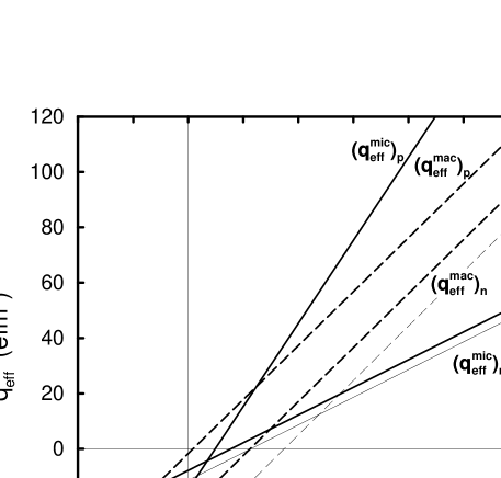
Figure 1: Effective electric quadrupole moments, $q_{eff}$, versus the single-particle mass quadrupole moment, $q_{\nu}$, at superdeformation, derived in the HO in the case when one particle is added to an orbital just above the gap. Solid and dashed lines are used for microscopic and macroscopic $q_{eff}$, respectively. Thick lines are used for the $g=40$ gap and thin lines for the $g=80$ gap (only drawn for neutrons). Very similar behaviour appears (not shown) when one particle is removed from an orbital just below the gap, i.e. $\Delta$ in eq. (34) is of minor importance.

Equations (2.2) are valid for arbitrary k values. They are illustrated for the superdeformed ($k=2$) $g=40$ gap ($N_{sh}=5$) in Fig. 1. There we have primarily chosen to put the particle in an orbital above the gap with ($N_{osc},n_{z}$) = (6,6), (5,4), etc. As $\left(q_{eff}^{mac}\right)_{p}$ has $a_{0}$ $=$ $0$ (which holds for all selfconsistent gaps) $\Delta^{mac}$ is directly seen as the deviation from 0 for $q_{\nu}=0$. All $a$-values are negative, i.e. the$q_{eff}$-values are all negative for $q_{\nu}=0$. This is easily understood from the fact that the quadrupole moment of an added particle to a superdeformed core must be sufficiently large to induce an increased deformation.

The slopes for the microscopic $q_{eff}$ are the same as for the spherical case, i.e. $(b^{mic})_{p}=1.5$ and $(b^{mic})_{n}=0.5$. The slopes, i.e. the $b$-values, in the macroscopic case depend on both $k$ and $g$ but, as illustrated in Fig. 2, in a way so that they

Figure 2: Values of $b^{mac}$ (i.e. the slope of the dashed lines in Fig. 1.) as functions of number of particles of each kind ($Z=N$) in the nucleus. The stars connected by solid lines are the 1st, 2nd, 3rd … selfconsistent gaps for each of the deformations: spherical ($1:1$), superdeformed ($2:1$) and hyperdeformed ($3:1$). One can see that the values converge to an asymptotic value close to one (see text for details), and that it requires the same number of selfconsistent gaps (i.e. more particles at larger deformation) to get the asymptotic value. The circles show the values of the slopes for deformations ($1:2$, $2:3$ and $3:2$) where there are no selfconsistent gaps. Note that all values are quite close to the value at the asymptotic limit and that, as explained in the text, the differences from this value can largely be understood from the choice of the parameter $\hbar$$\stackrel{{\scriptstyle o}}{{\omega}}_{0}$.

are almost constant and close to one for all gaps (except for the very lowest ones). The $b^{mac}$-values are the same e.g. for $g=40$ at $2:1$ as for $g=20$ at $1:1$ (and $g=60$ at $3:1$). These are the third lowest selfconsistent gaps at each deformation.

Using eq. (18) with the standard value of $D=41$ MeV an asymptotic value of 0.995 is found for $b^{mac}$ when N${}_{sh}\longrightarrow\infty$. It turns out, however, that the deviation from 1 is simply related to the value chosen for $D$. This value is generally determined so that $R_{rms}=1.2A^{1/3}$ fm , see e.g. [Nil95], leading to $D=41.2$ MeV with one digit higher accuracy. Using this value of $D$ instead gives $b^{mac}=1.000$ in the limit $N_{sh}\longrightarrow\infty$. Furthermore, if when deducing $D$, we do not go to the asymptotic limit but require that $R_{rms}=1.2A^{1/3}$ fm for each HO configuration, $\hbar$$\stackrel{{\scriptstyle o}}{{\omega}}_{0}$ will depend on $g/k$ in such a way that $b^{mac}\equiv 1$ for all selfconsistent gaps at $k:1$ deformation. Consequently, in these cases Fig. 2 just shows the effect of a constant $\hbar$$\stackrel{{\scriptstyle o}}{{\omega}}_{0}$ for all particle numbers at each deformation. However, as $D=41$ MeV is generally used in MO calculations independent of particle number, we think it is interesting to illustrate the effect which this $A$-dependence leads to for the polarization of an added particle. In particular this means that, in microscopic calculations, $R_{rms}$ will be larger than $1.2A^{1/3}$ fm for light nuclei.

At spherical shape $q_{eff}=0$ for $q_{\nu}=0$, i.e. $a=0$, as seen in eq. (2.2) ($k=1$). For prolate shape $\left(a^{mic}\right)_{p,n}$ and $(a^{mac})_{n}$ are negative. In Fig. 3

Figure 3: Dependence of $a^{mac}$ and $a^{mic}$ on deformation $\varepsilon$. The values are given for $g=40$ but, as the values scale with the number of particles in the same way as the single-particle quadrupole moment, $a/q_{\nu}$ is (asymptotically) independent of the number of particles. The different behaviour for particles and holes ($\Delta$ in eq. (34)) has been ignored.

is shown how $a$ varies with quadrupole deformation for a fixed number of particles. For $1:1$, $2:1$ and $3:1$ deformation we have used the selfconsistent gaps while for $1:2$, $2:3$ and $3:2$ deformation we have used the gaps whose deformation at minimal total energy is closest to the ‘correct’ deformation. For all deformations we have fitted a curve as a function of particle number (which becomes almost linear) to get the values at $g=40$.

In the high-$N_{sh}$ limit and for selfconsistent gaps we get the asymptotic relations defining the macroscopic effective quadrupole moments,

$$\left(b^{mac}\right)_{p} = \left(b^{mac}\right)_{n}=0.995$$

$$\left(a^{mac}\right)_{p} = -\left(0\pm 0.423\frac{k^{2}-1}{k^{4/3}}g^{1/3}\right)$$ (35)

$$\left(a^{mac}\right)_{n} = -\left(0.914\frac{k^{2}-1}{k^{2/3}}g^{2/3}\pm 0.423\frac{k^{2}-1}{k^{4/3}}g^{1/3}\right),$$

and the microscopic effective quadrupole moments,

$$\left(b^{mic}\right)_{p} = 1.5$$

$$\left(b^{mic}\right)_{n} = 0.5$$

$$\left(a^{mic}\right)_{p} = -\left(0.613\frac{k^{2}-1}{k^{2/3}}g^{2/3}\pm 0.212\frac{k^{2}-1}{k^{4/3}}g^{1/3}\right)$$ (36)

$$\left(a^{mic}\right)_{n} = -\left(0.306\frac{k^{2}-1}{k^{2/3}}g^{2/3}\pm 0.212\frac{k^{2}-1}{k^{4/3}}g^{1/3}\right).$$

It is clearly seen that $a_{0}$ (eq. (34)) increases with $g^{2/3}$ ($\propto A^{2/3}$) which is the same growth rate as for $q_{\nu}$, and therefore the relative importance of $a_{0}$ is independent of particle-number. The polarization difference between particles and holes, $\Delta$, on the other hand gets less important the heavier the nucleus is as it only increases as $g^{1/3}$.

Note that although the functions for macroscopic and microscopic $q_{eff}$ are quite different, the sum of the $q_{eff}$ values when adding one neutron and one proton is much more alike. This means that the total electric quadrupole moment for a nucleus with $Z\approx N$ is approximately the same independently of if the microscopic or the macroscopic formula is used.

The different behaviour of macroscopic and microscopic effective quadrupole moments have the same origin in the deformed case as the spherical case, and is caused by the two basically different assumptions applied. In the macroscopic approach, the protons as well as the neutrons are assumed to have a constant matter distribution inside the potential, i.e. also the matter distribution for protons and neutrons have identical deformations. Consequently, for a $Z=N$ nucleus the addition of a proton or neutron has the same polarization effect, except for a constant factor caused by the added charge, i.e. same $b$- but different $a$-parameters, as seen in eq. (2.2) for a deformation corresponding to a $k:1$ prolate shape. Independent of deformation, we asymptotically obtain $\left(b^{mac}\right)_{p}=\left(b^{mac}\right)_{n}\approx 1$, see eq. (35) (see also Fig. 1 for the k=2 case).

To analyze the microscopic approach, we start from identical proton and neutron configurations corresponding to an equilibrium deformation $\varepsilon_{o}$. Then if a proton is added, the isolated proton system will get a new equilibrium deformation which we will refer to as $\varepsilon_{o}+\delta\varepsilon$. The deformation of the combined system is then $\varepsilon_{o}+\delta\varepsilon/2$. The equilibrium deformation of the isolated neutron system is unchanged, $\varepsilon_{o}$. The electric quadrupole moment is then calculated at the (non-selfconsistent) deformation $\varepsilon_{o}+\delta\varepsilon/2$. From eq, (12), it is easy to find out that in a pure proton system, half of the change in the quadrupole moment will be caused by the changed value of $\varepsilon$, and half of the change by the change in the $\Sigma$’s. In the present case with a proton added to a $Z=N$ system, the change in the $\Sigma$’s for the protons is the same as when a proton is added to a pure proton system while the change in deformation for the total system (the polarization) is half of that for the pure proton system. This gives $\left(b^{mic}\right)_{p}=1.5$. If instead a neutron is added, there is no contribution from the change in the $\Sigma$’s as they refer to the proton-configuration, but the deformation of the total system will still be $\varepsilon_{o}+\delta\varepsilon/2$, and the contribution from this change in deformation will thus be the same. This gives $\left(b^{mic}\right)_{n}=0.5$, see eq. (36) (see also Fig. 1 for the k=2 case).

The difference between the macroscopic and microscopic polarizations are thus caused by the lack of selfconsistency when the isolated proton and neutron systems have different equilibrium deformations. Then, in the macroscopic approach, it is assumed that the proton and neutron matter distributions fully adopt the common deformation while they only do it ’halfway’ in the microscopic approach. With the assumption that the proton-proton, neutron-neutron and proton-neutron attractions are the same, it seems that the microscopic approach should come close to a fully selfconsistent treatment. However, a stronger attraction between unlike particles would correspond to a polarization in the direction suggested by the macroscopic approach.

In subsections 3.1 and 3.3 we calculate $q_{eff}$ in both methods for the modified oscillator potential, and in subsection 3.5 we compare the two methods with experimental data. First we will however study the polarization effects in the HO with a $Z\neq N$ core.

2.3 Quadrupole moments with a $Z\neq N$ core.

How will the results from the previous subsection change when the number of protons is far from the same as the number of neutrons? We will not derive all the formulae again but just investigate how different quantities depend on $Z$ and $N$. To analyse quadrupole moments, the correct equilibrium deformation of the proton-neutron system has to be obtained. This is done by minimizing the total energy $E(\varepsilon,Z,N)$. The energy of the proton system or neutron system can be written as

$$E_{i}=3\hbar\stackrel{{\scriptstyle o}}{{\omega}}_{0i}\left(\frac{1}{4}\Sigma_{\perp j}^{2}\Sigma_{zj}\right)^{1/3}\hskip 28.45274pt;\hskip 28.45274ptj=p,n.$$ (37)

We know that $\hbar$$\stackrel{{\scriptstyle o}}{{\omega}}_{0}$ follows eq. (19), and $\Sigma_{\perp}$ and $\Sigma_{z}$ are proportional to $Z^{4/3}$ and $N^{4/3}$ for protons and neutrons, respectively. Altogether the energy becomes

$$E_{p} \propto \frac{Z^{5/3}}{A^{2/3}}$$

$$E_{n} \propto \frac{N^{5/3}}{A^{2/3}}$$ (38)

for the two different systems. In a region around their respective equilibrium deformation the proton and the neutron energies can be well approximated with parabolas. The total energy, which is just the sum of the two energies, can therefore be written

$$E_{tot}=E_{0p}+C_{p}(\varepsilon-\varepsilon_{p})^{2}+E_{0n}+C_{n}(\varepsilon-\varepsilon_{n})^{2},$$ (39)

where the equilibrium deformation of each subsystem is

$$\varepsilon_{i}=\frac{3(2\Sigma_{zj}-\Sigma_{\perp j})}{4\Sigma_{zj}+\Sigma_{\perp j}}\hskip 28.45274pt;\hskip 28.45274ptj=p,n$$ (40)

and the energies at the minima ($E_{0p}$ and $E_{0n}$) and the stiffness parameters ($C_{p}$ and $C_{n}$), all with proportionality according to eq. (38), determine each parabola. By minimizing the total energy, $E_{tot}$, the equilibrium deformation of the total system is obtained as

$$\varepsilon_{0}=\frac{C_{p}\varepsilon_{p}+C_{n}\varepsilon_{n}}{C_{p}+C_{n}}=\frac{Z^{5/3}\varepsilon_{p}+N^{5/3}\varepsilon_{n}}{Z^{5/3}+N^{5/3}}.$$ (41)

The $b$ values describe the part of $q_{eff}$ which depends on single particle properties of the added particle (eq. (33)). They enter via the change $\delta\varepsilon$ in equilibrium deformation, and for protons in the microscopic case by a direct contribution of 1 $q_{\nu}$. The change in total quadrupole moment caused by the deformation change is to first order

$$\delta Q_{def}\propto ZA^{2/3}\delta\varepsilon,$$ (42)

while the single-particle quadrupole moment is

$$q_{\nu p} \propto \frac{A^{2/3}}{Z^{1/3}}f(\sigma_{zp},\sigma_{\perp p})$$

$$q_{\nu n} \propto \frac{A^{2/3}}{N^{1/3}}f(\sigma_{zn},\sigma_{\perp n}),$$ (43)

where $f(\sigma_{zp},\sigma_{\perp p})$ and $f(\sigma_{zn},\sigma_{\perp n})$ are independent of $Z$ and $N$. In total we get the expressions

$$\left(\frac{\delta Q_{def}}{q_{\nu}}\right)_{p} \propto \frac{ZA^{2/3}\frac{Z^{5/3}}{Z^{5/3}+N^{5/3}}\frac{3(2\sigma_{zp}-\sigma_{\perp p})}{4\Sigma_{zp}+\Sigma_{\perp p}}}{A^{2/3}Z^{-1/3}f(\sigma_{zp},\sigma_{\perp p})}=\frac{Z^{5/3}}{Z^{5/3}+N^{5/3}}F(\sigma_{zp},\sigma_{\perp p})$$

$$\left(\frac{\delta Q_{def}}{q_{\nu}}\right)_{n} \propto \frac{ZA^{2/3}\frac{2N^{5/3}}{Z^{5/3}+N^{5/3}}\frac{3(2\sigma_{zn}-\sigma_{\perp n})}{4\Sigma_{zn}+\Sigma_{\perp n}}}{A^{2/3}N^{-1/3}f(\sigma_{zn},\sigma_{\perp n})}=\frac{Z}{N}\frac{N^{5/3}}{Z^{5/3}+N^{5/3}}F(\sigma_{zn},\sigma_{\perp n}).$$ (44)

where $F(\sigma_{zp},\sigma_{\perp p})$ and $F(\sigma_{zn},\sigma_{\perp n})$ are independent of $Z$ and $N$. The previously derived $b$-values (eqs. (35,36)) can now be generalized to any proton-neutron system

$$\left(b^{mac}(Z,N)\right)_{p} = \frac{2Z^{5/3}}{Z^{5/3}+N^{5/3}}\left(b^{mac}(Z_{0}=N_{0})\right)_{p}$$

$$\left(b^{mac}(Z,N)\right)_{n} = \frac{Z}{N}\frac{2N^{5/3}}{Z^{5/3}+N^{5/3}}\left(b^{mac}(Z_{0}=N_{0})\right)_{n}$$

$$\left(b^{mic}(Z,N)\right)_{p} = 1+\frac{2Z^{5/3}}{Z^{5/3}+N^{5/3}}\left(\left(b^{mic}(Z_{0}=N_{0})\right)_{p}-1\right)$$ (45)

$$\left(b^{mic}(Z,N)\right)_{n} = \frac{Z}{N}\frac{2N^{5/3}}{Z^{5/3}+N^{5/3}}\left(b^{mic}(Z_{0}=N_{0})\right)_{n}$$

keeping in mind that the $Z=N$ $b$-values were only deduced for selfconsistent gaps, but should be approximately valid for all $Z$- and $N$-values. For the nucleus ${}^{152}$Dy the predictions from the HO is $b^{mac}_{p}=0.78$, $b^{mac}_{n}=0.93$, $b^{mic}_{p}=1.39$, and $b^{mic}_{n}=0.47$.

3 Quadrupole moments at superdeformation in the cranked MO potential.

We will now continue to analyze polarization effects on quadrupole moments in the cranked MO model. Starting from the superdeformed ${}^{152}$Dy configuration, we shall study how the quadrupole moment is affected by adding or removing protons or neutrons in specific orbitals. Contrary to the previous section, all calculations are performed at $I\approx 40\hbar$. It has previously been concluded [Rag80] that at superdeformation, the general properties of the single-particle orbitals are almost unaffected by spin up to the highest observed values $I=60-70\hbar$. Furthermore, our present study shows that the polarizing properties in the HO at superdeformation are essentially the same at $I=0\hbar$ and at $I=40\hbar$. In subsections 3.1 and 3.2 we study the macroscopic quadrupole moments, which have been used in recent comparisons with experiment and seem to work quite well [Sav96, Nis97], while similar calculations using the microscopic quadrupole moments are carried out in subsections 3.3 and 3.4. We perform a complete calculation in the cranked MO potential (parameters from ref. [Haa93]) with Strutinsky renormalization to get the proper equilibrium deformation, $\varepsilon$ and $\varepsilon_{4}$, of each configuration. The formalism of ref. [Ben85] is used which makes it straightforward to study specific configurations defined by the number of particles of signature $\alpha=1/2$ and $\alpha=-1/2$, respectively, in the different $N_{rot}$ shells of the rotating HO basis. The macroscopic electric quadrupole moment, $Q^{mac}$, is obtained from an integration over the volume described by the nuclear potential and the microscopic electric quadrupole moment, $Q^{mic}$, by adding the contributions $q_{\nu}$ from the occupied proton orbitals at the proper deformation. One-particle polarization effects are investigated in subsections 3.1 and 3.3 while the additivity of several particles is studied in subsections 3.2 and 3.4. In subsection 3.5 the two theoretical methods are compared and confronted with experiment.

3.1 Macroscopic polarization effects of one-particle states

In the present study, we first calculate the macroscopic quadrupole moments $Q^{mac}$ in neighbouring nuclei which only differ by one particle or one hole from the yrast superdeformed configuration in ${}^{152}$Dy. From these $Q^{mac}$-values effective electric quadrupole moments, $q_{eff}$, are obtained for different orbitals. For the orbitals around the $Z=66$ and $N=86$ gaps, $q_{eff}$ is plotted vs. the mass single-particle quadrupole moment, $q_{\nu}$, in Fig. 4 (see also Table 4 below).

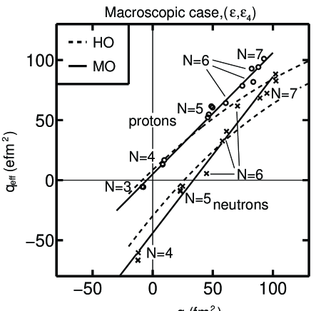
Figure 4: Changes in the total macroscopic quadrupole moment, $q_{eff}$, when a particle is added to or removed from the superdeformed core plotted vs. the single-particle mass quadrupole moment, $q_{\nu}$. The circles and crosses are obtained from calculations in the Strutinsky-renormalized cranked MO with simultaneous energy-minimization in $\varepsilon$ and $\varepsilon_{4}$ direction using ${}^{152}$Dy as a core (values are given in Table 4). The quantum number $N\equiv N_{rot}$ is indicated for each state. The solid lines, whose equations are given in the text, are linear least square fits to the respective points. The dashed lines are the quadratic least square fits for the HO potential (with $\varepsilon_{4}$ deformation included) with the ($Z=60,N=80$) core, as defined in Fig. 5.

It is evident that these values define approximate straight lines. By a least square fit we get the relation

$$q_{eff}=(1.02q_{\nu}+5.4)\;e{\rm fm}^{2}$$ (46)

for protons and

$$q_{eff}=(1.30q_{\nu}-43.7)\;e{\rm fm}^{2}$$ (47)

for neutrons. This should be compared with $b^{mac}_{p}=0.78$ and $b^{mac}_{n}=0.93$ obtained from eqs. (35,45). It is evident that there are important differences.

Let us analyze the differences between the $Z=N$ HO and the MO results for ${}^{152}$Dy by introducing, in the numerical calculations, the different terms one at the time. Starting with the $Z=N$ HO we get the expected modifications when combining the HO superdeformed gaps $Z=60$ and $N=80$: Due to the neutron excess the average slope gets notably smaller than in the $Z=N$ case and neutrons have a larger slope than protons, all in agreement with eq. (45). Cranking the system and performing a Strutinsky renormalization (i.e. including macroscopic liquid drop energy) only have a minor effect on the slopes, see dashed lines in Fig. 5.

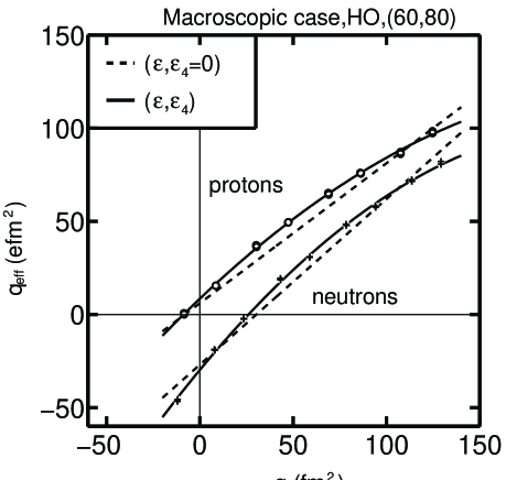
Figure 5: Changes in the total macroscopic quadrupole moment, $q_{eff}$, when a particle is added to or removed from the $Z=60$ and $N=80$ core plotted vs. the single-particle mass quadrupole moment, $q_{\nu}$. The curves are least square fits to the calculations in Strutinsky-renormalized cranked HO calculations. The dashed lines show the relations when the energy is minimized only in $\varepsilon$ deformation with $\varepsilon_{4}=0$. The solid lines (corresponding proton and neutron data marked with circles and crosses, respectively) show the relations when the energy is simultaneously minimized in the $\varepsilon$ and $\varepsilon_{4}$ directions.

In the standard HO only quadrupole deformation $\varepsilon$ is used, while in the MO the energy is minimized in the quadrupole and hexadecapole deformation plane. In order to test the importance of the hexadecapole $\varepsilon_{4}$-deformation it is now included in the (cranked and Strutinsky-renormalized) HO, see the solid lines in Fig. 5. Due to the hexadecapole $\varepsilon_{4}$-deformation there is now a curvature in the relation $q_{eff}=q_{eff}(q_{\nu})$, but the best linear fit is very close to the one obtained for quadrupole deformation only.

When changing to the MO potential by including the $\vec{l}\cdot\vec{s}$ and $l^{2}$-terms, there are large changes, see Fig. 4. The large differences between the HO and the MO are understood by considering the stiffness of the core in the two models. Around the equilibrium quadrupole deformation $\varepsilon_{0}$ of the core, its energy can be expressed as

$$E_{core}=E_{0}(\varepsilon_{0})+C(\varepsilon-\varepsilon_{0})^{2},$$ (48)

and the energy of the added particle as

$$e_{part}=e_{0}(\varepsilon_{0})+K(\varepsilon-\varepsilon_{0}).$$ (49)

The change in deformation of the total system, due to the added particle, is therefore $K/2C$. The stiffness $C$ of the energy surface is larger for the HO than for the MO (see below), and this directly gives a larger deformation change in the MO for the same single particle quadrupole moment (same $K$). Consequently, in the MO the total quadrupole moment will increase more for high-$N_{osc}$ orbitals with a positive deformation change and decrease more for low-$N_{osc}$ orbitals with negative deformation change. The slope of $q_{eff}(q_{\nu})$ will therefore be considerably larger in the MO than in the HO.

The net result of the change from the HO with a $Z=N$ core to the cranked MO potential with the $Z=66$, $N=86$ core is thus an increase in the slope of the $q_{eff}$ vs. $q_{\nu}$ relation for neutrons, but almost no change in the proton slope. Furthermore, the relations still become approximately linear also in the MO case.

One might ask why the polarization effects are larger in the MO than in the HO. To investigate this, we carried out calculations in the HO both with the HO closed shell configuration ($Z=60,N=80$), and for the configuration corresponding to the yrast superdeformed band in ${}^{152}$Dy. It turned out that, when corrected for the difference in mass, the different configurations had very similar stiffness. Calculations were then carried through for the ${}^{152}$Dy configuration with only the $l^{2}$-term or the $\vec{l}\cdot\vec{s}$-term included, indicating that the $l^{2}$-term is responsible for approximately 60 % and the $\vec{l}\cdot\vec{s}$-term for 40 % of the change in stiffness.

3.2 Additivity of macroscopic effective quadrupole moments

It is now interesting to investigate if the $q_{eff}$ values are additive, i.e. if quadrupole moments of several-particle several-hole configurations relative to the superdeformed ${}^{152}$Dy yrast state (with the $Q^{mac}$ value 1893 $e$fm${}^{2}$) can be calculated from the formula

$$Q_{est}=Q\left({}^{152}Dy_{yrast}\right)+\sum\limits_{particle}q_{eff}-\sum\limits_{hole}q_{eff}.$$ (50)

The additivity will first be tested for excited states in ${}^{152}$Dy where the number of excited particles are the same as the number of excited holes. We shall then test the additivity in other superdeformed nuclei all the way down to ${}^{142}$Sm.

Starting with ${}^{152}$Dy, we give in Table 1 calculated deformations and quadrupole moments for a few $n$-particle $n$-hole configurations with rather low excitation energy. The quadrupole moments are calculated both by exact integration and by use of eq. (50) with $q_{eff}$ taken from the 1-hole or 1-particle configurations given in Fig. 4. The agreement between these two methods is good with a typical difference of 2 $e$fm${}^{2}$.

Table 1: Calculated deformations and macroscopic quadrupole moments for SD configurations of ${}^{152}$Dy. The two values of the quadrupole moment are obtained from a numerical integration ($Q_{exact}$) and by adding and subtracting $q_{eff}$ values to the yrast quadrupole moment ($Q_{est}$). The values of $q_{eff}$ are obtained from 1-particle or 1-hole configurations relative to the yrast state, see Fig. 4 and Table 4 below.

Configurations of ${}^{152}$Dy.	$Q_{exact}$	$Q_{est}$	$\varepsilon$	$\varepsilon_{4}$
	($e$fm${}^{2}$)	($e$fm${}^{2}$)
yrast	1893.2		0.5820	0.0166
$\pi([651]3/2^{-})^{-1}([413]5/2^{-})$	1826.9	1828	0.5716	0.0211
$\pi([301]1/2^{-})^{-1}([532]3/2^{-})$	1960.6	1960	0.6012	0.0282
$\nu([770]1/2^{+})^{-1}([402]5/2^{+})$	1749.1	1750	0.5519	0.0135
$\pi([651]3/2^{-})^{-1}([651]3/2^{+})^{-1}$
$([413]5/2^{-})([413]5/2^{+})$	1765.2	1766	0.5608	0.0241
$\pi([651]3/2^{-})^{-1}([651]3/2^{+})^{-1}$
$([532]3/2^{-})([413]5/2^{-})$	1809.1	1811	0.5706	0.0259
$\pi([651]3/2^{-})^{-1}([413]5/2^{-})$
$\nu([770]1/2^{+})^{-1}([402]5/2^{-})$	1686.4	1685	0.5415	0.0182
$\pi([651]3/2^{-})^{-1}([651]3/2^{+})^{-1}$
$([532]3/2^{-})([413]5/2^{+})$	1726.9	1723	0.5601	0.0388
$\nu([770]1/2^{+})^{-1}([521]3/2^{-})$

Considering the good agreement between the ‘exact’ and ‘estimated’ macroscopic quadrupole moments for ${}^{152}$Dy, one could ask if similar methods could be used to estimate the quadrupole moment for other SD nuclei around ${}^{152}$Dy. Furthermore, considering the approximately linear relation between $q_{\nu}$ and $q_{eff}$ discussed above, it is interesting to investigate if these quadrupole moments can be obtained from a knowledge of $Q$ for the reference nucleus and $q_{\nu}$ (but not $q_{eff}$) for the active orbitals. Quadrupole moments for configurations in the nuclei ${}^{150}$Dy, ${}^{148}$Dy, ${}^{150}$Gd, ${}^{148}$Gd, ${}^{144}$Gd, ${}^{143}$Eu and ${}^{142}$Sm were therefore calculated in three different ways:

• By direct calculation at the appropriate equilibrium deformation; $Q_{exact}$ in Table 2.

• From the quadrupole moment of the superdeformed ${}^{152}$Dy yrast state and the sum of effective one-hole quadrupole moments; $Q_{est}(q_{eff})$ in Table 2.

• From the quadrupole moment of the superdeformed ${}^{152}$Dy yrast state and the sum of effective quadrupole moments calculated from single-particle quadrupole moments by the simple linear relations eqs. (46,47); $Q_{est}(q_{\nu})$ in Table 2.

Table 2: Macroscopic quadrupole moments calculated in three different ways (see text) for SD configurations in selected nuclei with one or several holes relative to the ${}^{152}$Dy reference nucleus.

nucleus	configuration relative	$Q_{exact}$	$Q_{est}(q_{eff})$	$Q_{est}(q_{\nu})$	$Q_{exact}-Q_{est}(q_{\nu})$
	SD ${}^{152}$Dy yrast	($e$fm${}^{2}$)	($e$fm${}^{2}$)	($e$fm${}^{2}$)	($e$fm${}^{2}$)
${}^{152}$Dy		1893
${}^{150}$Dy	$\nu 7^{-2}$	1725	1722	1715	10
${}^{150}$Gd	$\pi 6^{-2}$	1735	1733	1722	13
${}^{148}$Dy	$\nu 6^{-4}$	1701	–	1714	$-13$
${}^{148}$Gd	$\pi 6^{-2}\nu 7^{-2}$	1576	1562	1544	32
${}^{144}$Gd	$\pi 6^{-2}\nu 7^{-2}6^{-4}$	1381	–	1365	16
${}^{143}$Eu	$\pi 6^{-3}\nu 7^{-2}6^{-4}$	1305	–	1277	28
${}^{142}$Sm	$\pi 6^{-3}([541]1/2)^{-1}\nu 7^{-2}6^{-4}$	1232	–	1198	34
${}^{142}$Sm	$\begin{array}[]{l}\pi 6^{-2}([541]1/2)^{-1}3^{-1}\\ \nu 7^{-1}6^{-4}([411]1/2)^{-1}\end{array}$	1419	–	1410	9

When choosing the configurations, we have to make sure that if two orbitals interact in the superdeformed region, both these orbitals should be either empty or occupied. This is the reason why the four $N=6$ neutron orbitals (2 of each signature) are treated as one entity.

In Table 2, $Q_{est}(q_{eff})$ values are presented only for configurations which have holes in the orbitals used to get the effective one-hole quadrupole moments plotted in Fig. 4 while $Q_{est}(q_{\nu})$ are calculated for all configurations. The two estimates based on $q_{eff}$ and $q_{\nu}$, respectively, differ by up to 18 $e$fm${}^{2}$ for four particles removed. The difference between the calculated value, $Q_{exact}$, and the single-particle estimate $Q_{est}(q_{\nu})$ is at most 34 $e$fm${}^{2}$. The corresponding rms-value is 22 $e$fm${}^{2}$ for all configurations in Table 2. It is astonishing that the summation of effective quadrupole moments, calculated from eqs. (46, 47), describes the ‘exactly’ calculated values within 2% for ${}^{142}$Sm, which is ten particles away from ${}^{152}$Dy, and where the deformation has changed from $\varepsilon=0.58$ to $\varepsilon=0.48$ and $\varepsilon=0.52$ for the two studied configurations.

The two ${}^{142}$Sm configurations included have been measured in experiment [Hac98] and comparison with these data will be discussed in subsection 3.5. In the Sm-bands, there are two orbitals which have to be handled with extra care. Thus, due to the difference in deformation the order of some orbitals closest to the Fermi-surface are different in ${}^{152}$Dy and ${}^{142}$Sm. At the deformation of ${}^{152}$Dy, the proton $N_{osc}=5$ and neutron $N_{osc}=4$ closest to the Fermi-surface are $\pi([532]5/2)$ and $\nu([404]9/2)$, i.e. the corresponding points in Fig. 4 are constructed from configurations with holes in these orbitals. At the deformation of the Sm-bands on the other hand, the $\pi([541]1/2)$ and $\nu([411]1/2)$ orbitals are higher in energy and therefore, the bands are formed with holes in these orbitals relative to the ${}^{152}$Dy bands. Consequently, their single-particle moments should be used in the relations to get the quadrupole moments in ${}^{142}$Sm, see Table 2. The orbitals are relatively pure in the ${}^{142}$Sm configurations because, at the relevant rotational frequencies, the crossings between the orbitals occur at deformations somewhere between that of ${}^{152}$Dy and ${}^{142}$Sm. Therefore, these configurations are anyway a good test on how well additivity, based on $q_{\nu}$, works 10 particles away from ${}^{152}$Dy.

3.3 Microscopic polarization effects of one-particle states

In a similar way as in section 3.1 we now calculate the microscopic quadrupole moments $Q^{mic}=e\sum_{\nu=1}^{Z}q_{\nu}$ in neighbouring nuclei to superdeformed ${}^{152}$Dy and plot $q_{eff}$ vs. $q_{\nu}$, see the solid lines in Fig. 6.

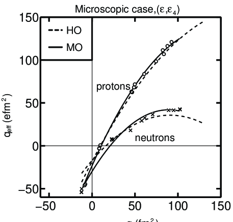
Figure 6: Changes in the total microscopic quadrupole moment, $q_{eff}$, when a particle is added to or removed from the superdeformed core plotted vs. the single-particle mass quadrupole moment, $q_{\nu}$. The circles and crosses are obtained from calculations in the Strutinsky-renormalized cranked MO with simultaneous energy-minimization in the $\varepsilon$ and $\varepsilon_{4}$ directions using ${}^{152}Dy$ as a core (values are given in Table 4). The solid lines are quadratic least square fits to these points. The dashed lines are obtained from analogous fits for the HO potential with the ($Z=60,N=80$) core, as defined in Fig. 7.

Using the full MO, the relations no longer are approximatively linear but rather quadratic,

$$q_{eff}=(-0.008q_{\nu}^{2}+2.28q_{\nu}-23.3)e{\rm fm}^{2}$$ (51)

for protons and

$$q_{eff}=(-0.009q_{\nu}^{2}+1.61q_{\nu}-30.0)e{\rm fm}^{2}$$ (52)

for neutrons. This might suggest that it would be more proper to express $q_{eff}$ not only as a function of the single-particle quadrupole moment, but also of the hexadecapole moment. However, as found below, the relations eqs. (51) and (52) seem to work well in the limited region of superdeformed nuclei with $A=142-152$, so at present we will make no attempt to generalize eqs. (51) and (52).

In a similar way as in the macroscopic case, the reason why the microscopic relations are so different from what was found in the $Z=N$ HO calculations is now analyzed by performing calculations where the different terms in the full MO relative to the HO are introduced one at a time.

First, allowing a different number of protons and neutrons and calculating also for non-selfconsistent gaps give linear relations with changes in the slopes in accordance with eq. (45). Introducing the Strutinsky renormalization and cranking only has a minor effect on the $q_{eff}$ vs. $q_{\nu}$ relations.

The result of including hexadecapole deformation $\varepsilon_{4}$ in the HO is shown in Fig. 7.

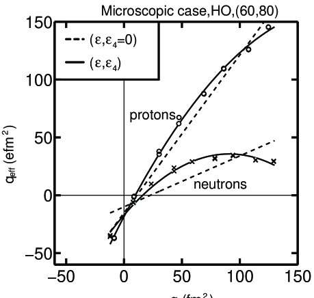
Figure 7: Changes in the total microscopic quadrupole moment, $q_{eff}$, when a particle is added to or removed from the $Z=60$ and $N=80$ core plotted vs. the single-particle mass quadrupole moment, $q_{\nu}$. The curves are least square fits to the calculations in Strutinsky-renormalized cranked HO calculations. The dashed lines show the relation when the energy is minimized only in $\varepsilon$ deformation with $\varepsilon_{4}=0$. The solid lines (corresponding proton and neutron data marked with circles and crosses, respectively) show the relation when the energy is simultaneously minimized in the $\varepsilon$ and $\varepsilon_{4}$ directions.

As in the macroscopic case (see Fig. 5), the hexadecapole deformation introduces a curvature, which is, however, more than twice as large in this microscopic case. In Fig. 6 the MO result is compared to the HO result, both including the hexadecapole deformation. The two curves are seen to be rather similar, although the stronger polarization effect for the MO than for the HO, discussed above for the macroscopic case, can be seen also in the microscopic case. Furthermore, there is a small increase of the curvature of the $q_{eff}$ vs. $q_{\nu}$ relation.

The reason why the introduction of the $\vec{l}\cdot\vec{s}$ and $l^{2}$-terms rather increase the curvature in the microscopic case (Fig. 6) but removes the curvature in the macroscopic case (Fig. 4) is not understood.

3.4 Additivity of microscopic effective quadrupole moments

The additivity in the microscopic case is checked, see Table 3, in the same way as in the macroscopic case, i.e. the electric quadrupole moment is calculated in three different ways $Q_{exact}$, $Q_{est}(q_{eff})$, and $Q_{est}(q_{\nu})$, as described in subsection 3.2.

The result of this test is that the additivity seems to work with a similar accuracy in this model as in the macroscopic approach. This is illustrated in Fig. 8 where

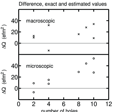
Figure 8: The difference between the calculated and estimated (based on $q_{\nu}$) quadrupole moment as a function of number of holes relative to the superdeformed ${}^{152}$Dy core. The upper panel shows the macroscopic result from Table 2 while the lower panel shows the corresponding microscopic result from Table 3.

the difference between the calculated, $Q_{exact}$, and the single particle estimated quadrupole moments, $Q_{est}(q_{\nu})$, is plotted as a function of number of holes relative to the superdeformed ${}^{152}$Dy core.

For the three configurations where the quadrupole moment has been estimated based on both $q_{eff}$ and $q_{\nu}$, the maximum deviation is 7 $e$fm${}^{2}$, see Table 3. The rms value for $Q_{exact}-Q_{est}(q_{\nu})$ is 29 $e$fm${}^{2}$ for the eight configurations considered in Table 3, while the maximum deviation is 53 $e$fm${}^{2}$. In the microscopic case, summing effective quadrupole moments, calculated from eqs. (51, 52), describes the two ${}^{142}$Sm configurations with a 4 % accuracy.

Table 3: Microscopic quadrupole moments calculated for SD configurations in selected nuclei with one or several holes relative to the ${}^{152}$Dy reference nucleus.

nucleus	configuration relative	$Q_{exact}$	$Q_{est}(q_{eff})$	$Q_{est}(q_{\nu})$	$Q_{exact}-Q_{est}(q_{\nu})$
	SD ${}^{152}$Dy yrast	($e$fm${}^{2}$)	($e$fm${}^{2}$)	($e$fm${}^{2}$)	($e$fm${}^{2}$)
${}^{152}$Dy		1810
${}^{150}$Dy	$\nu 7^{-2}$	1722	1725	1729	$-7$
${}^{150}$Gd	$\pi 6^{-2}$	1607	1605	1598	9
${}^{148}$Dy	$\nu 6^{-4}$	1675	–	1660	15
${}^{148}$Gd	$\pi 6^{-2}\nu 7^{-2}$	1528	1520	1517	8
${}^{144}$Gd	$\pi 6^{-2}\nu 7^{-2}6^{-4}$	1396	–	1367	29
${}^{143}$Eu	$\pi 6^{-3}\nu 7^{-2}6^{-4}$	1303	–	1259	44
${}^{142}$Sm	$\pi 6^{-3}([541]1/2)^{-1}\nu 7^{-2}6^{-4}$	1213	–	1160	53
${}^{142}$Sm	$\begin{array}[]{l}\pi 6^{-2}([541]1/2)^{-1}3^{-1}\\ \nu 7^{-1}6^{-4}([411]1/2)^{-1}\end{array}$	1395	–	1367	28

3.5 Comparison between macroscopic, microscopic and experimental effective quadrupole moments

The two models studied give quite simple relations (eqs. (46, 47) and eqs. (51, 52)) between $q_{eff}$ and $q_{v}$, but their predictions for specific orbitals are rather different as can be seen in Fig. 9.

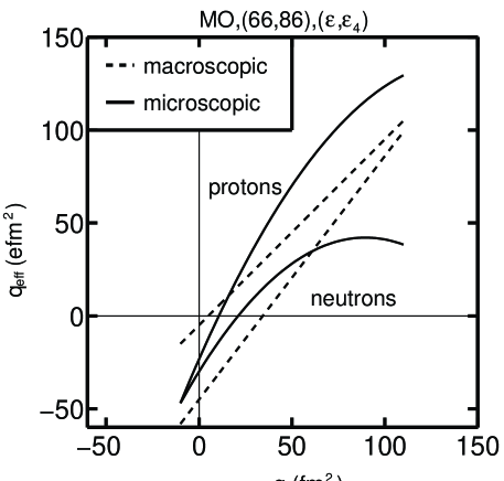
Figure 9: Effective electric quadrupole moments versus single-particle mass quadrupole moments calculated in the MO for one particle/hole outside the superdeformed ${}^{152}$Dy core. Dashed lines are used for the macroscopic and solid lines for the microscopic method. It is clear that for specific combinations of protons and neutrons removed from the ${}^{152}$Dy core, the two methods could lead to rather different results.

In the macroscopic relations neutrons and protons with high $q_{\nu}$-value have similar effects, while the microscopic relations give very different values for protons and neutrons, with exception for the lowest $q_{\nu}$-values. In the microscopic case for neutrons the maximum $q_{eff}$ is not obtained from the maximum $q_{\nu}$. In Table 4 $q_{\nu}$ and $q_{eff}$-values are given for several different orbitals close to the Fermi-surface in ${}^{152}$Dy. The $q_{eff}$-values are shown both for the macroscopic and the microscopic case. For comparison values from Skyrme-Hartree-Fock calculations are also presented. By using these effective quadrupole moments together with eq. (50) (with the scalings discussed below) electric quadrupole moments can be estimated for a large number of superdeformed configurations in a rather large region around ${}^{152}$Dy. There are also configurations with only $q_{\nu}$-values given. From those one can estimate effective electric quadrupole moments by using eqs. (46,47) and eqs. (51,52), and through eq. (50) get good estimates of electric quadrupole moments for many more configurations in this region.

Table 4:

Effective quadrupole moments calculated for orbitals in the SD $A=150$ region. The macroscopic and microscopic values, calculated in ${}^{152}$Dy $\pm$ 1 particle, are the ones used when producing Fig. 4 and Fig. 6. For other orbitals only $q_{\nu}$-values is given. They can be used together with the relations eqs. (46, 47) and eqs. (51, 52) to estimate macroscopic and microscopic effective quadrupole moments. The Skyrme-Hartree-Fock calculations are from ref. [Sat96].

orbital $q_{\nu}$ $q^{mac}_{eff}$ $q^{mic}_{eff}$ $q^{SkP}_{eff}$ $q^{SkM^{*}}_{eff}$ orbital $q_{\nu}$ $q^{mac}_{eff}$ $q^{mic}_{eff}$ $q^{SkP}_{eff}$ $q^{SkM^{*}}_{eff}$ ($e$fm${}^{2}$) ($e$fm${}^{2}$) ($e$fm${}^{2}$) ($e$fm${}^{2}$) ($e$fm${}^{2}$) ($e$fm${}^{2}$) ($e$fm${}^{2}$) ($e$fm${}^{2}$) ($e$fm${}^{2}$) ($e$fm${}^{2}$) proton holes neutron holes $\pi([301]1/2^{-})^{-1}$ -7.8 -5.7 -44.8 -15 -18 $\nu([404]9/2^{-})^{-1}$ -12.3 -66.5 -54.0 $\pi([301]1/2^{+})^{-1}$ -8.6 -5.5 -46.1 -18 -16 $\nu([404]9/2^{+})^{-1}$ -12.3 -66.8 -54.3 $\pi([413]7/2^{-})^{-1}$ 8.3 13.6 -3.0 $\nu([523]7/2^{-})^{-1}$ 23.0 -8.5 7.9 $\pi([413]7/2^{+})^{-1}$ 8.3 13.0 -3.3 $\nu([523]7/2^{+})^{-1}$ 23.0 -9.3 7.3 $\pi([532]5/2^{-})^{-1}$ 46.7 54.7 63.2 $\nu([642]5/2^{-})^{-1(a)}$ 58.0 32.6 29.2 22 22 $\pi([532]5/2^{+})^{-1}$ 45.9 52.3 62.4 $\nu([642]5/2^{+})^{-1(a)}$ 70.6 61.7 36.6 24 24 $\pi([651]3/2^{-})^{-1}$ 83.7 81.8 106.9 96 96 $\nu([770]1/2^{-})^{-1}$ 102.3 88.3 42.7 59 48 $\pi([651]3/2^{+})^{-1}$ 74.6 78.5 98.5 89 88 $\nu([770]1/2^{+})^{-1}$ 102.6 82.6 42.3 57 48 $\pi([541]1/2^{-})^{-1}$ 71.6 $\nu([411]1/2^{-})^{-1}$ 8.7 18 16 $\pi([541]1/2^{+})^{-1}$ 68.3 $\nu([411]1/2^{+})^{-1}$ 9.4 15 13 $\pi([660]1/2^{-})^{-1}$ 81.4 $\nu([651]1/2^{-})^{-1(a)}$ 78.5 43 28 $\pi([660]1/2^{+})^{-1}$ 84.6 $\nu([651]1/2^{+})^{-1(a)}$ 66.1 43 30 proton particles neutron particles $\pi([413]5/2^{-})$ 9.6 16.7 0.6 $\nu([402]5/2^{-})$ -12.0 -60.4 -50.2 -44 -38 $\pi([413]5/2^{+})$ 9.6 16.7 10.6 $\nu([402]5/2^{+})$ -12.0 -60.4 -50.2 -44 -38 $\pi([532]3/2^{-})$ 48.8 61.5 70.2 $\nu([521]3/2^{-})$ 24.9 -5.0 7.4 0 -1 $\pi([532]3/2^{+})$ 49.9 60.5 71.7 $\nu([521]3/2^{+})$ 24.9 -5.0 7.4 0 -1 $\pi([642]5/2^{-})$ 82.4 92.9 111.5 $\nu([640]1/2^{-})$ 44.8 5.5 18.0 $\pi([642]5/2^{+})$ 60.8 64.2 83.7 $\nu([640]1/2^{+})$ 61.5 40.6 32.6 $\pi([770]1/2^{-})$ 92.6 101.1 121.0 $\nu([761]3/2^{-})$ 89.2 68.4 41.5 46 41 $\pi([770]1/2^{+})$ 87.9 94.1 116.4 $\nu([761]3/2^{+})$ 95.0 72.3 41.5 41 28 (a) The orbitals $\nu([642]5/2)$ and $\nu([651]1/2)$ are mixed in the Dy-region and are not pure in ${}^{152}$Dy. If none or both orbitals of the same parity is unoccupied the quadrupole moment can be correct calculated from these values, else extra care should be taken. The labels are valid for the Skyrme-Hartree-Fock values.

Table 5: Macroscopic and microscopic quadrupole moments are compared with experiments. The holes are specified relative to the reference, superdeformed ${}^{152}$Dy yrast configuration.

nucleus	configuration relative	$Q^{exp}$	$0.92Q^{mac}$	$0.96Q^{mic}$	$Q^{exp}-0.92Q^{mac}$	$Q^{exp}-0.96Q^{mic}$
	SD ${}^{152}$Dy yrast	($e$b${}^{2}$)	($e$b${}^{2}$)	($e$b${}^{2}$)	($e$b${}^{2}$)	($e$b${}^{2}$)
${}^{152}$Dy		17.5${}^{a)}$	17.4	17.4	0.1	0.1
${}^{151}$Dy	$\nu 7^{-1}$	16.9${}^{b)}$	16.6	17.0	0.3	$-0.1$
${}^{151}$Tb	$\pi 6^{-1}$	16.8${}^{a)}$	16.6	16.3	0.2	0.5
${}^{149}$Gd	$\pi 6^{-2}\nu 7^{-1}$	15.0${}^{a)}$	15.2	15.1	$-0.2$	$-0.1$
${}^{149}$Gd	$\pi 6^{-2}\nu 6^{-1}$	15.6${}^{a)}$	15.4	15.1	0.2	0.5
${}^{149}$Gd	$\nu 6^{-1}3^{-1}\nu 7^{-1}$	15.2${}^{a)}$	16.0	16.2	$-0.8$	$-1.0$
${}^{149}$Gd${}^{d)}$	$\pi 3^{-2}\nu 4^{-1}$	17.5${}^{a)}$	17.7	18.3	0.2	$-0.8$
${}^{148}$Gd	$\pi 6^{-2}\nu 7^{-1}6^{-1}$	14.6${}^{a)}$	14.7	14.7	$-0.1$	$-0.1$
${}^{148}$Gd	$\pi 6^{-2}\nu 7^{-1}6^{-1}$	14.8${}^{a)}$	14.7	14.7	0.1	0.1
${}^{148}$Gd${}^{d)}$	$\pi 3^{-2}\nu 4^{-2}$	17.8${}^{a)}$	18.0	18.5	$-0.2$	$-0.7$
${}^{142}$Sm	$\pi 6^{-3}5^{-1}\nu 7^{-2}6^{-4}$	11.7${}^{c)}$	11.3	11.6	0.4	0.1
${}^{142}$Sm${}^{e)}$	$\pi 6^{-2}5^{-1}3^{-1}\nu 7^{-1}6^{-4}4^{-1}$	13.2${}^{c)}$	13.1	13.4	0.1	$-0.2$

The experimental data are from ${}^{a)}$ ref. [Sav96], ${}^{b)}$ ref. [Nis97], ${}^{c)}$ ref. [Hac98]. In the configurations marked ${}^{d)}$ the hole is forced to the $\nu([411]1/2)^{-1}$ orbit in order not to mix with $\nu([404]9/2)^{-1}$ orbit while in the configuration marked ${}^{e)}$ the hole naturally comes in the $\nu([411]1/2)^{-1}$ orbit.