Modeling Pionic Fusion

Abstract

Recently observed rare heavy ion fusion processes, where the entire available energy is carried away by a single pion, is an example of extreme collectivity in nuclear reactions. We calculate the cross section in the approximation of sudden overlap, modeling the initial and final nuclei by moving harmonic oscillator potentials. This allows for a fully quantum-mechanical treatment, exact conservation of linear and angular momenta and fulfillment of the Pauli principle. The results are in satisfactory agreement with data. Mass number dependence and general trends of the process are discussed.

I Introduction

Nuclear fusion reactions which produce a pion are often referred to as pionic fusion. Pion production has been observed [1, 2, 3] at energies approaching absolute threshold, where the entire available energy is converted into the pion, demonstrating an amazing collective behavior of nucleon systems. However it remains quite difficult to incorporate the observed collectivity into existing theoretical models. A variety of studies [4, 5, 6, 7] have dealt with subthreshold pion production in heavy ion collisions, where the energy per nucleon is below the energy threshold of the elementary single-particle reaction $NN\rightarrow NN+\pi$. Most models, such as those featuring pion bremsstrahlung mechanisms [8, 9], quantum molecular dynamics approaches[10], perturbative calculations using Boltzmann-Nordheim-Vlasov equations [11] or nuclear structure functions [12], provide a good picture at energies starting from $E/A\approx 30$ MeV up to the single-particle threshold $E/A=280$ MeV in the laboratory frame. In the present work motivated by the experimental results of [1, 2, 3] our aim is to consider even lower energies and study the behavior of the cross section of fusion reaction in the region down to $\approx$10 MeV above the absolute threshold. This necessitates a careful consideration of limitations on the reaction given by conservation laws and the Pauli exclusion principle which govern the behavior of the cross section in this extreme situation. The statistical approach used in most existing models at higher energy has to be substituted by low energy many-body structure physics.

Our model, that is described in the Sect. II, considers the cross section in the Born approximation, assuming that pion production occurs through coupling to a single nucleon. All possible further rescatterings of the pion are expected to significantly reduce the probability of the reaction, and are ignored as higher order processes. A schematic picture of the reaction is shown in Fig. 1 demonstrating the pionic fusion of two nuclei $A$ and $A^{\prime}$.

FIG. 1.: The pionic fusion of two nuclei in the sudden approximation is illustrated.

Many-body nuclear mean field parameters are assumed to be constant and suddenly change from the initial to the final values. This will be referred to as the sudden approximation. The three-dimensional harmonic oscillator shell model is used to describe the structure of the incoming and outgoing nuclei. This allows analytical calculation of all necessary overlap amplitudes. The stationary wave functions are constructed as Slater determinants projected onto good angular momentum. Taking into account the center-of-mass motion we preserve linear momentum. Sect. III shows the implementation of the model for the case of pionic fusion of two identical nuclei. In Sect. IV we present a low pion momentum approximation, for which more general results could be derived. The parallel discussion of mathematical details is given in the Appendices. The application of this model to experimentally observed pionic fusion reactions shows a good agreement with data. The comparison is presented in Sect. V along with some predictions for heavy nuclei.

II Description of the model

A The transition amplitude

We approach the problem of pionic fusion as a stationary scattering problem. We consider the reaction cross section to be given by the Fermi golden rule in terms of the transition amplitude $\langle F|H|I\rangle$, where $I$ and $F$ refer to the initial and final states, respectively, of the whole system including the emitted pion. The density of final pion states is given by $Vk^{2}dk\,d\Omega/(2\pi)^{3}$ with $k$ as a momentum of the pion produced; $\Omega$ is a solid angle in the center of mass (CM) frame, and $V$ stands for the quantization volume. In all further calculations the pion is assumed to be fully relativistic whereas nucleons obey non-relativistic quantum mechanics. We use a set of natural units with $\hbar=c=1$. In this framework the differential cross section can be written as

$$d\sigma={\omega km\over 2p_{n}(2\pi)^{2}}|\langle F|H|I\rangle|^{2}V^{2}d\Omega\quad,$$ (1)

where $m$ is a nucleon mass, $p_{n}$ is the CM momentum per nucleon in the initial state and $\omega=\sqrt{k^{2}+m_{\pi}^{2}}$ is pion energy.

On the single-nucleon level one can use a phenomenological Hamiltonian density for the pion-nucleon interaction [13],

$${\cal H}=g{\overline{\psi}}{\gamma_{5}}{\vec{\tau}}\psi{\vec{\pi}}+4\pi{\lambda_{1}\over m_{\pi}}\bar{\psi}{\vec{\pi}}\cdot{\vec{\pi}}\psi+4\pi{\lambda_{2}\over m_{\pi}^{2}}\bar{\psi}{\bf r}\cdot{\vec{\pi}}\times\dot{\vec{\pi}}\psi\quad.$$ (2)

A number of studies have been performed analyzing this form of the interaction within the context of chiral perturbation theory [14]. The first term, often called in the literature the impulse or Born term, is responsible for single-pion production in a $p$-wave. We neglect the second and the third $s$-wave terms which require an additional interaction to absorb the extra pion created in the four-point vertex. We believe that due to the difficulty of recombining the nucleons into an appropriate final state the second and third terms become increasingly unimportant for larger nuclei. It has also been experimentally observed that in the pionic fusion reactions the pion is predominantly produced in the $p$-wave [1, 2]. Reduction of the first term in the Hamiltonian to a non-relativistic case gives an interaction of the form

$$\Gamma=g{{\vec{\sigma}}\cdot{\bf{k}}\over 2m}\quad,$$ (3)

with the coupling $g$ appropriately defined according to isospin. Separation of the quantized pion field,

$$\pi(x)=\sum_{k}{1\over{\sqrt{2\omega V}}}(a_{k}^{+}e^{-i{\bf k}\cdot{\bf x}}+a_{k}e^{+i{\bf k}\cdot{\bf x}}),$$ (4)

in the matrix element of Eq. (1) reduces the transition amplitude to the following form

$$\langle F|H|I\rangle={1\over{\sqrt{2\omega V}}}{1\over 2m}\,\langle f|\sum_{{\rm nucleons}}g\,{\bf k}\cdot{\vec{\sigma}}e^{-i{\bf k}\cdot{\bf x}}|i\rangle\quad,$$ (5)

where $|f\rangle$ and $|i\rangle$ are final and initial states of the nucleon system.

B Nuclear wave functions

We will approximate a state of a nuclear system with an antisymmetric combination built upon single-particle (s.p.) states. We take these states from the harmonic oscillator shell model, which allows for the analytic calculation of corresponding overlaps. The approach however can be extended to any single-particle basis. Each of the single-particle states can be characterized by the number of excitation quanta in three Cartesian directions, the nucleon spin and isospin projections. The locations of the centers of the harmonic oscillator potentials for all separate nuclei have to be introduced as additional parameters to the wave function. The importance of these parameters in projecting a nucleon wave function onto a state with correct total momentum for every nucleus participating in the process is discussed below. Following these assumptions we will write the wave function of a nucleon system as follows

$$|\underbrace{({\vec{\alpha}}_{1},s_{1},t_{1};{\vec{\alpha}}_{2},s_{2},t_{2};\ldots;{\bf r})}_{{\rm nucleus}\,A},\underbrace{(\overbrace{{\vec{\alpha}}_{A+1},s_{A+1},t_{A+1}}^{(A+1){\rm th\,\,s.p.\,\,state}};{\vec{\alpha}}_{A+2},s_{A+2},t_{A+2};\ldots;{\bf r}^{\,\prime})}_{{\rm nucleus}\,A^{\prime}}\rangle\quad.$$ (6)

In this example we assume that the system consists of two nuclei $A$ and $A^{\prime}$ with the centers of their respective harmonic oscillator potentials at ${\bf r}$ and ${\bf r^{\,\prime}}$. The single-particle orbitals are numbered from $1$ to $A$ for the first nucleus and from $A+1$ up to the total number of nucleons $A_{f}=A+A^{\prime}$ for the second one. Labels ${\vec{\alpha}}=(\alpha_{x},\alpha_{y},\alpha_{z})$ are Cartesian quantum numbers of single-particle states, while $s$ and $t$ are the spin and isospin projections. Protons and neutrons can be considered separately as well as different spin projections of the nucleons, reducing the wave function of the state to a product of four components. If the described separation is performed and the resulting part of the wave function contains only single-particle states with the same values of either $s$ or $t$ then the corresponding index is omitted in writing. We use a standard form for the one-dimensional harmonic oscillator wave functions centered at $r$ in the coordinate representation:

$$\langle x|(\alpha;r)_{v}\rangle=\sqrt{v\over\sqrt{\pi}2^{\alpha}{\alpha}!}\,H_{\alpha}(v(x-r))e^{-v^{2}(x-r)^{2}/2}\quad.$$ (7)

The parameter $v$ is defined for a single oscillator as $v=\sqrt{m\omega}$. These parameters characterize the mean field potentials for every incoming or outgoing nucleus. The function $H_{n}(x)$ is the $n$th order Hermite polynomial of the variable $x$. The discussion of the overlap integrals such as $\langle(\alpha^{\prime},r^{\,\prime})_{v^{\prime}}|(\alpha,r)_{v}\rangle$, and the general form of the results is presented in Appendix A.

A simple projecting technique was used to construct wave functions as eigenstates of the momentum operators that correspond to the total momenta of each individual nucleus,

$$|({\vec{\alpha}}_{1},s_{1},t_{1};\ldots;{\bf p}),({\vec{\alpha}}_{A+1},s_{A+1},t_{A+1};\ldots;{\bf p}^{\,\prime})\rangle=$$ (8)

$${\cal N}^{-1}\,\int\int_{-\infty}^{+\infty}d^{3}r\,d^{3}r^{\,\prime}\,|({\vec{\alpha}}_{1},s_{1},t_{1};\ldots;{\bf r}),({\vec{\alpha}}_{A+1},s_{A+1},t_{A+1};\ldots;{\bf r}^{\,\prime})\rangle e^{i({\bf p}\cdot{\bf r}+{\bf p}^{\,\prime}\cdot{\bf r}^{\,\prime})}\quad.$$ (9)

It is easy to check that

$$-i\sum_{j=1}^{A}{\bf\nabla}_{j}|({\vec{\alpha}}_{1},\ldots;{\bf p}),({\vec{\alpha}}_{A+1},\ldots;{\bf p}^{\,\prime})\rangle={\bf p}\,|({\vec{\alpha}}_{1},\ldots;{\bf p}),({\vec{\alpha}}_{A+1},\ldots;{\bf p}^{\,\prime})\rangle$$ (10)

and

$$-i\sum_{j=A+1}^{A+A^{\prime}}{\bf\nabla}_{j}|({\vec{\alpha}}_{1},\ldots;{\bf p}),({\vec{\alpha}}_{A+1},\ldots;{\bf p}^{\,\prime})\rangle={\bf p}^{\,\prime}\,|({\vec{\alpha}}_{1},\ldots;{\bf p}),({\vec{\alpha}}_{A+1},\ldots;{\bf p}^{\,\prime})\rangle\quad.$$ (11)

In the above example the situation with two-nuclei state is shown, which is appropriate for describing the initial state in pionic fusion. The final state containing just one fused nucleus is constructed analogously.

Due to the finite range of the interaction, the overall normalization ${\cal N}$ of the state (9) that contains several moving nuclei, is just a product of normalizations for each of the constituent nuclei individually. It is useful to write the CM coordinates separately from the relative coordinates of the nucleons

$$|({\vec{\alpha}}_{1};{\vec{\alpha}}_{2};\ldots{\vec{\alpha}}_{A};{\bf r})_{v}\rangle=|({\vec{\alpha}}_{\rm CM}=(0,0,0);{\bf r})_{v\sqrt{A}}\rangle\,|\psi_{\rm rel}\rangle\quad.$$ (12)

The relative coordinate wave function $|\psi_{\rm rel}\rangle$ can be complicated but the CM part for the ground state nucleus is simply represented by the unphysical ground state oscillation of the center of mass in the effective harmonic potential with the parameter $v\sqrt{A}$. This is removed by a projection (9) onto the correct momentum state. The normalization integral can be expressed as

$${\cal N}^{2}=\int\int d^{3}r\,d^{3}r^{\,\prime}\langle({\vec{\alpha}}_{\rm CM};{\bf r}^{\,\prime})_{v\sqrt{A}}|({\vec{\alpha}}_{\rm CM};{\bf r})_{v\sqrt{A}}\rangle\,\langle\psi_{\rm rel}|\psi_{\rm rel}\rangle e^{i{\bf p}({\bf r}-{\bf r}^{\,\prime})}$$ (13)

$$=\int d^{3}r\int d^{3}r^{\,\prime}e^{-A({\bf r}-{\bf r}^{\,\prime})^{2}v^{2}/4}e^{i{\bf p}({\bf r}-{\bf r}^{\,\prime})}=\left({4\pi\over v^{2}A}\right)^{3/2}Ve^{-{p^{2}/Av^{2}}}\quad.$$ (14)

A different method of calculating the normalization along with further justification of this form for the CM part of the wave function is discussed in Appendix B. We also note here that with a slight modification of Eq. (14) the orthogonality of the nucleon wave functions can be shown

$$\langle({\vec{\alpha}}_{1};{\vec{\alpha}}_{2};\ldots{\vec{\alpha}}_{A};{\bf p}^{\prime})_{v}|({\vec{\alpha}}_{1};{\vec{\alpha}}_{2};\ldots{\vec{\alpha}}_{A};{\bf p})_{v}\rangle={\cal N}^{2}\delta_{{\bf p},\,{\bf p}^{\prime}}\,.$$

III Fusion reactions $A+A\rightarrow 2A+\pi$

For the remainder of the paper we will assume $A$ to be the mass number of each of the initial nuclei with proton-neutron composition ($Z$,$N$) and $w$ the oscillator parameter. The entire initial state is characterized by a set of the single-particle quantum numbers $\{{\vec{\alpha}}_{i}\}$. The fusion product has $2A=A_{f}$ nucleons, the oscillator parameter $v$, and the final state quantum numbers $\{{\vec{\beta}}_{i}\}$. The collision is considered in the CM reference frame; therefore we use ${\bf p}$ and $-{\bf p}$ to denote the momenta of the incoming nuclei and ${\bf k}$ for a final pion momentum with corresponding ${\bf p}_{f}=-{\bf k}$ as the total momentum of the recoil nucleus. The integration of the wave functions leading to correct momenta, Eq. (9), is performed at a final stage so initially overlaps are calculated as functions of ${\bf r}$ , ${\bf r}^{\,\prime}$ and ${\bf R}$, the locations of the centers of the two initial nuclei and the final nucleus, respectively.

A Charged pion production

We begin with the case of $\pi^{+}$ production where one of the initial protons interacts with the pion field producing a neutron and a real on-shell pion. With the assumption that the pion was produced in a single-particle interaction, the total amplitude of the process becomes a sum over all possible amplitudes shown in Fig. 2, with the pion vertex connecting any of the initial protons to any of the final state neutrons with the correct relative sign to preserve antisymmetry.

FIG. 2.: One of the amplitudes of the total fusion process: an initial proton from the $n$th orbit produces a $\pi^{+}$ and ends at the $l$th final neutron single-particle orbit. $F_{n}$ is the remaining overlap of a proton system with the $n$th initial single-particle state missing. $G_{l}$ is the neutron overlap with no $l$th state in the final system.

Suppose the interacting proton in the single-particle state $n$ produced a neutron in the state $l$ of the final nucleus. In the initial state we sum over the occupied orbitals of the first and the second colliding nucleus, for $n\leq Z$ and for $Z<n\leq 2Z$, respectively. We use the notations $G_{l}(r,r^{\prime},R)$ for the neutron overlap

$$G_{l}=\langle\underbrace{({\vec{\beta}}_{1},\tilde{s}_{1};\ldots{\vec{\beta}}_{l-1},\tilde{s}_{l-1};{\vec{\beta}}_{l+1},\tilde{s}_{l+1};\ldots;{\bf R})}_{{\rm no\,}l{\rm th\,s.p.\,state}}|({\vec{\alpha}}_{1},s_{1};\ldots;{\bf r})({\vec{\alpha}}_{A+1},s_{A+1};\ldots;{\bf r^{\,\prime}})\rangle\,,$$ (15)

$F_{n}(r,r^{\prime},R)$ for the proton overlap

$$F_{n}=\langle({\vec{\beta}}_{1},\tilde{s}_{1};\ldots;{\bf R})|\underbrace{({\vec{\alpha}}_{1},s_{1};\ldots;{\vec{\alpha}}_{n-1},s_{n-1};{\vec{\alpha}}_{n+1},s_{n+1};\ldots)}_{{\rm no\,}n{\rm th\,s.p.\,state}}\rangle\,,$$ (16)

and $H_{n\,l}$ for a single-particle matrix element

$$H_{n\,l}=\left\{\matrix{\langle({\vec{\beta}}_{l},\tilde{s}_{l};{\bf R})|g\,{\vec{\sigma}}\cdot{\bf k}\,e^{-i{\bf k}\cdot{\bf x}}|({\vec{\alpha}}_{n},s_{n};{\bf r})\rangle\qquad n\leq Z\cr\langle({\vec{\beta}}_{l},\tilde{s}_{l};{\bf R})|g\,{\vec{\sigma}}\cdot{\bf k}\,e^{-i{\bf k}\cdot{\bf x}}|({\vec{\alpha}}_{n},s_{n};{\bf r}^{\,\prime})\rangle\qquad n>Z\cr}\right.\,.$$ (17)

Finally, following Eq.(5), the total amplitude can be expressed in terms of the following sum:

$$\langle F|H|I\rangle={1\over{\cal N}_{i}{\cal N}_{f}}{1\over{\sqrt{2\omega V}}}{1\over 2m}\int\int d^{3}r\,d^{3}r^{\prime}\,d^{3}R\,\sum_{nl}(-1)^{n+l}F_{n}G_{l}H_{nl}e^{i{\bf p}({\bf r}-{\bf r}^{\,\prime})-i{\bf p}_{f}\cdot{\bf R}}\,.$$ (18)

The determinants of the matrices are constructed from a product of the single-particle overlaps of size $(2N)\times(2N)$ for the neutrons ($G_{l}$) and $(2Z-1)\times(2Z-1)$ for the protons ($F_{n}$). The Gaussian nature of the single-particle overlaps allows one to separate all exponential factors that govern the general trend of the cross section leaving only some polynomials of a general form that carry spin, isospin and Pauli blocking information. These mathematical manipulations are discussed in some detail in Appendix B. Here we present a final expression for the square of the transition amplitude

$$|\langle F|H|I\rangle|^{2}={2g^{2}\over V^{2}}\left({2\pi\over v^{2}A}\right)^{3/2}{|{\bf k}|^{2}\,\xi\over\omega m^{2}}\,\eta^{6(A-1)}\left|M_{+}\right|^{2}\,,$$ (19)

in which the exponential factor $\xi$, effective oscillator parameter $\eta$ and reduced amplitude $M_{+}$ are introduced as follows

$$\xi\equiv\exp{\left(-{2p^{2}\over Av^{2}}-{k^{2}\over v^{2}+w^{2}}-{k^{2}(w^{2}-v^{2})\over 2Av^{2}(v^{2}+w^{2})}\right)}\quad,$$ (20)

$$\eta\equiv{2vw\over v^{2}+w^{2}}\quad,$$ (21)

and

$$M_{+}\equiv P(k,p)e^{{{\bf p}\cdot{\bf k}}/Av^{2}}+Q(k,p)e^{-{{\bf p}\cdot{\bf k}}/Av^{2}}\,.$$ (22)

Here, $P$ and $Q$ are dimensionless polynomials of $p$ and $k$, the total CM momentum of the initial nuclei and the final pion momentum. The polynomials are to be determined using particular configurations of the initial and final nuclei. They are also functions of $v$ and $w$ which determine the appropriate momentum scale. If the two colliding nuclei have the same initial shell model state then $P(k,p)=\pm Q(k,-p)$ (the phase difference given by $\pm$ sign for even or odd $Z$, respectively, is due to imposed Pauli antisymmetry, see Appendix B). The procedure of analytically calculating $P$ and $Q$ involves finding the determinant of the matrix constructed from polynomials that result from integrating a product of Hermite polynomials of the form $\langle(\beta,R)|(\alpha,r)\rangle$; and performing the integrational Fourier-type conversion, Eqs. (9). This process is discussed in Appendix B. The size of the matrices is determined by the number of nucleons of the same spin-isospin type.

B Neutral pion production

The case of $\pi^{0}$ production can be considered in a similar fashion. A neutral pion can be produced either by one of the protons or by one of the neutrons, which couple with a negative relative sign. Compared to charged pions the coupling is larger by a factor $\sqrt{2}$. The final amplitude can then be expressed, similarly to Eq. (19), as

$$|\langle F|H|I\rangle|^{2}={g^{2}\over V^{2}}\left({2\pi\over A\,v^{2}}\right)^{3/2}{|{\bf k}|^{2}\,\xi\over\omega m^{2}}\,\eta^{6(A-1)}\left|M_{0}\right|^{2}\,.$$ (23)

Here the reduced amplitude can be split into a proton and a neutron part:

$$M_{0}=P_{p}(k,p)e^{{\bf p\cdot k}/Av^{2}}+Q_{p}(k,p)e^{-{\bf p\cdot k}/Av^{2}}-P_{n}(k,p)e^{{\bf p\cdot k}/Av^{2}}-Q_{n}(k,p)e^{-{\bf p\cdot k}/Av^{2}}\,.$$ (24)

IV Low pion momentum approximation

Due to the specific form of the polynomials discussed above, further simplifications can be made for the case of $\pi^{0}$ production. Near the absolute threshold, the pion momentum $|{\bf k}|$ is small compared to all other momentum parameters $|{\bf p}|$, $v$ and $w$, and can be ignored in polynomials. Then

$$H_{n\,l}=\langle({\vec{\beta}}_{l},s_{l};{\bf R})_{v}|{\vec{\sigma}}\cdot{\bf k}\,e^{-i{\bf k}\cdot{\bf x}}|({\vec{\alpha}}_{n},s_{n};{\bf r})_{w}\rangle$$ (25)

$$\approx\langle s_{l}|{\vec{\sigma}}\cdot{\bf k}|s_{n}\rangle\,\langle({\vec{\beta}}_{l};{\bf R})_{v}|({\vec{\alpha}}_{n};{\bf r})_{w}\rangle\exp\left({\frac{-k^{2}}{2(v^{2}+w^{2})}}-{\frac{i{\bf k}\cdot({\bf R}v^{2}+{\bf r}w^{2})}{(v^{2}+w^{2})}}\right)\,.$$ (26)

With this approximation, the interaction part is factorized into exponents as shown in the expression above. Therefore the total pionic fusion amplitude is a product of a pure fusion amplitude and the expression that arises from the operator ${\vec{\sigma}}\cdot{\bf k}$ acting on the nucleons. For a given type of the initial and final nucleon, the sum of a single-particle matrix element multiplied by the corresponding overlap of the remaining particles reduces to a sum of matrix elements multiplied by the corresponding minor which is related to a determinant of a full matrix. It is shown in Appendix C that the polynomials can be expressed in an analytical form if all inner harmonic oscillator shells are completely filled without any gaps in all participating nuclei. This restriction allows any type of particle-hole excitations within the outer unfilled shell.

The total differential cross section for a neutral pion production close to absolute threshold is given in the form:

$${d\sigma\over d\Omega}={g^{2}Ak^{3}\over(2\pi)^{2}2pm}\left({2\pi\over A\,v^{2}}\right)^{3/2}\,\eta^{6(A-1)+{\cal Q}_{f}+{\cal Q}_{i}}\left({4w\over Av}\right)^{{\cal Q}_{f}-{\cal Q}_{i}}e^{-{2p^{2}/Av^{2}}}\times$$ (27)

$$\left|\,2^{q_{z}/2}T_{q_{z}}\left({ip\sqrt{2\over A\eta vw}}\right){(q_{x}-1)!!\>(q_{y}-1)!!}\,\right|^{2}\,{1\over\gamma^{2}}\,\left|{\tilde{M}}\right|^{2}\quad.$$ (28)

Here the integers $q_{j},\,j=x,y,z$ are introduced as differences between numbers of quanta in final and initial systems for three Cartesian directions; ${\cal Q}_{i}$ and ${\cal Q}_{f}$ are total numbers of quanta in initial and final systems. These values are defined as

$$q_{j}=\sum_{\rm nucleons}{\beta}_{j}-\sum_{\rm nucleons}{\alpha}_{j}\,,\quad{\cal Q}_{i}=\sum_{\rm nucleons}(\alpha_{x}+\alpha_{y}+\alpha_{z})\,,\quad{\cal Q}_{f}=\sum_{\rm nucleons}(\beta_{x}+\beta_{y}+\beta_{z})\,.$$ (29)

The spin and radial parts of the wave function are completely decoupled in our non-relativistic description of the nucleon system. This allows to introduce the matrix element used in Eq. (28)

$${\tilde{M}}={1\over|{\bf k}|}\,\langle{\tilde{f}}|\sum_{\rm nucleons}\tau_{z}\,{\vec{\sigma}}\cdot{\bf k}|{\tilde{i}}\rangle\,,$$ (30)

where ${\tilde{i}}$ and ${\tilde{f}}$ are the spin-isospin parts of nucleon wave function of initial and final systems, respectively. This matrix element could be directly computed for every particular nuclear configuration, but for a large number of states degenerate within harmonic oscillator model it is useful to use an approximation for the average

$$\overline{{\tilde{M}}}\,=\,\overline{\left({Z_{\uparrow}-Z_{\downarrow}-N_{\uparrow}+N_{\downarrow}}\right)}\,.$$ (31)

The Cartesian directions of the harmonic oscillator quantization axes are chosen in such a way that the $z$ axis coincides with the beam direction, though the spin is quantized along the ${\bf k}$ axis that simplifies the action of ${\vec{\sigma}}\cdot{\bf k}$ which is used to obtain Eq. (31). Integers $Z_{\uparrow}$, $Z_{\downarrow}$, $N_{\uparrow}$ and $N_{\downarrow}$ are mean numbers of particles for each spin-isospin combination with respect to our axis of spin quantization. The polynomials $T_{n}(x)$, defined in Eq. (40) of Appendix A, can be approximated as

$$2^{q_{z}/2}T_{q_{z}}\left({ip\sqrt{2\over A\eta vw}}\right)\,\approx\,\left({ip\sqrt{2\over A\eta vw}}\right)^{q_{z}}\quad.$$ (32)

This approximation is valid in the limit that the arguments become large and allows for a better quantitative understanding of the behavior of the cross section. The value of the argument is almost independent of the mass number $A$ at threshold energy:

$$p\sqrt{2\over A\eta vw}\,\approx\,6\,.$$

In Eq. (28) only the lowest order term in the pion momentum is retained resulting in a $p$-wave cross section (exponents with $k$ are also ignored). The equation has only one numerical parameter $\gamma$, the origin of which is discussed in Appendix C. This parameter is a product of four factors, one for every spin/isospin nucleon species. Each factor depends on the number of particles of corresponding type and on their distribution within the highest harmonic oscillator shell for both initial and final nuclei. Numerically, $\gamma$ range from $1$ to $10$ for light nuclei. The cross section can be zero if some symmetries are not preserved (spin, isospin, oscillator symmetry) as well as by virtue of Eq. (43) in Appendix A if creation of the final system requires an odd number of quanta relative to the initial system in any of the transverse directions.

V Application of the model and results

A The reaction $p+p\rightarrow d+\pi^{+}$

The first and the simplest example to calculate is the two-nucleon fusion reaction $p+p\rightarrow d+\pi^{+}$. This example serves here only for illustrative purpose as we do not include pion rescattering due to the full interaction given by Hamiltonian density of Eq. (2) which is important for this elementary process. Moreover, the deuteron hardly can be approximated with the harmonic oscillator shell model. The polynomials $P$ and $Q$ in this case do not depend on $p$ being equal to the matrix element of ${\vec{\sigma}}\cdot{\bf k}/|{\bf k}|$ evaluated between the spinors of initial interacting proton and final neutron. In Eq. (19) we choose a minus sign for antisymmetry. Here, $P$ and $Q$ correspond to the choice of the first or second initial proton to produce a pion, respectively.

Dominant partial wave channels are summarized in the following table along with our results for their reduced amplitudes. The table was constructed by separation of initial singlet and triplet states of the $NN$ system. Partial waves of the $\pi-d$ system printed in the left column that yield the dominant contributions to the amplitudes which are shown in the right column.

$$\begin{array}[]{ccc}{\rm pion}&NN\,{\rm state}&{\rm amplitude}\\ \hline\cr s{\rm-wave}&{}^{3}P_{1}&2\,{\sqrt{2}}\,\sinh({\frac{k\,p\,\cos\theta}{A\,{v^{2}}}})\\ \begin{array}[]{c}p{\rm-wave}\\ p{\rm-wave}\end{array}&\left.\begin{array}[]{c}{}^{1}S_{0}\\ {}^{1}D_{2}\end{array}\right\}&2\,\cosh({\frac{k\,p\,\cos\theta}{A\,{v^{2}}}})\end{array}$$ (33)

As can be seen from the table above, this cross section is predominantly $p$-wave in nature at low pion energies. The $s$-wave contribution that comes [13] from rescattering of the pion due to the interaction (2) was not included. The total cross section averaged over spin projections in the initial state and summed over final states is

$${d\sigma\over d\Omega}={\frac{{g^{2}}\,k^{3}}{2\,m\,p\,{\sqrt{2\,\pi}}\,{v^{3}}}}\,{\exp\left(-{\frac{4\,{p^{2}}+k^{2}}{2\,{v^{2}}}}\right)}\left[3\,\cosh\left({\frac{2\,k\,p\,\cos\theta}{{v^{2}}}}\right)-1\right]\quad.$$ (34)

The obtained $p$-wave cross section behaves at low energies as

$$\sigma(pp\rightarrow d\pi^{+})=\tilde{\sigma}\left(k/m_{\pi}\right)^{3}\quad,$$ (35)

where

$$\tilde{\sigma}={2\sqrt{2\pi}g^{2}m_{\pi}^{5/2}\over m^{3/2}v^{3}}e^{-2mm_{\pi}/v^{2}}\quad.$$ (36)

Choosing the oscillator parameter $v=216$ MeV/c reproduces the experimental value[15], $4\tilde{\sigma}\approx 0.42$ fm². For this case the fusion is sensitive to the tail of the wave function in momentum space. Since the wave function of a deuteron is extremely non-Gaussian with a long tail in coordinate space, choosing $v$ to reproduce the deuteron’s r.m.s. charge radius would result in a grossly underpredicted cross section. For the fusion of heavier ions, the incoming nuclei are moving at a slower velocity and their momenta per nucleon are similar to characteristic momentum scales of the wave functions.

The oscillator parameter $v$ can be best obtained by matching used here harmonic oscillator type deuteron wave function to its experimentally known behavior [15]. The choice of this parameter between 180 and 220 fm would lead to the values of $4\tilde{\sigma}$ in the range of 0.06 to 0.48 fm².

B The reaction ³He $+$ ³He $\rightarrow$ ⁶Li $+$ $\pi^{+}$

As a next step, we apply the model to the experimentally studied pionic fusion reaction ³He $+$ ³He $\rightarrow$ ⁶Li $+$ $\pi^{+}$, where even first excited states of the ⁶Li nucleus have been resolved [2]. This reaction involves heavier nuclei so that the process of pion rescattering becomes less important as discussed above. The polynomials $P$ and $Q$ for Eq. (19) can be constructed in a direct way considering the shell model structure of all nuclei involved in the reaction. The ground $1^{+}$ and first excited $3^{+}$ states of ⁶Li were constructed within the $p_{3/2}$ j-subshell. In Fig. 3, the total cross section for this reaction is calculated for the fusion into the ground state (left panel) and the first excited state (right panel). The contributions of the $s$-wave and $p$-wave to the cross section are plotted together. We choose a value $v=118.91$ MeV/c for ⁶Li as it corresponds to the oscillator frequency of 15.06 MeV, the parameter of MK3W model [16]. The initial parameter $w=112.7$ MeV/c was chosen by assuming the r.m.s. size 2.14 fm of ³He. In Fig. 4 we show the differential cross section for this fusion reaction going into the ground state of ⁶Li (solid line) and the first excited state (dashed line). The beam energy is assumed to be fixed so that the corresponding absolute values of the pion momentum are $96$ and $90$ MeV/c, respectively.

Comparison with the experiment [2] in which pionic fusion resolves the few lowest levels of ⁶Li shows that we obtain a reasonable ratio of the cross sections. However, we underpredict the magnitude by approximately $40\%$, compared to the estimated experimental value of $111\pm 11$ nb for the ground state transition. We note that the result is sensitive to parameters of the shell model and their choice in the harmonic oscillator approximation is quite uncertain for light nuclei. For example, a variation of the final oscillator frequency within $10\%$ range of the used value would lead to the values of the cross section between about $20$ and $140$ nb. Using more realistic non-Gaussian wave functions might significantly improve the model. We might also be underestimating the cross section due to inherent limitations of the approach. For instance, we do not consider a gradual change of the nuclear mean field in the process of fusion substituting it with the sudden approximation.

FIG. 3.: Reaction cross sections for ³He $+$ ³He $\rightarrow$ ⁶Li $+$ $\pi^{+}$. The left panel shows the transition to the ground state and the right panel to the first excited state of ⁶Li at $2.18$ MeV. The solid lines represent the total cross section, dashed and dotted lines are $s$ and $p$-waves, respectively.

FIG. 4.: Differential cross section of the reaction ³He $+$ ³He $\rightarrow$ ⁶Li $+$ $\pi^{+}$. On the left panel the solid line represents the transition to the ground state of ⁶Li and the dashed line to the first excited state; the corresponding absolute values of pion momentum are 96 and 90 MeV/c, respectively. The right panel displays the experimentally observed values [2] of the differential cross section of the transition to the ground state (squares) and to the first excited state (circles) of ⁶Li.

C The reaction ¹²C + ¹²C $\rightarrow$ ²⁴Mg + $\pi^{0}$

Here we apply our approach to the cross section of the ¹²C + ¹²C $\rightarrow$ ²⁴Mg + $\pi^{0}$ reaction. This process, along with its isospin analog ¹²C + ¹²C $\rightarrow$ ²⁴Na + $\pi^{+}$, represents those few heavy ion pionic fusion reactions for which experimental data exist [1]. The application of the developed theory does not present a great difficulty except the fact that the cross section is quite dependent on the structure of initial and final states of interacting nuclei. Within the harmonic oscillator picture we have approximately $3\times 10^{8}$ different combinations of interacting states that correspond to the same energy. Angular momentum and isospin conservation constraints reduce this number by several orders of magnitude. Additional shell model interactions have to be introduced to build up a realistic nuclear state for each of the nuclei and reduce this large number of states, that are degenerate in our model, to the ones of interest. Based on this argument we will present here the Monte-Carlo averaged cross section, where we average over random Cartesian states. In the following Fig. 5 we display the total reaction cross section as a function of pion momentum. We use here the oscillator parameters $v=104$ MeV/c and $w=119$ MeV/c which are estimated by various theoretical models [17, 18].

FIG. 5.: The reaction cross section for ¹²C + ¹²C $\rightarrow$ ²⁴Mg + $\pi^{0}$ with oscillator parameters $v=104$ MeV/c and $w=119$ MeV/c as a function of pion momentum.

The experimentally estimated cross section for this reaction is $208\pm 38$ pb which was observed for pion momentum 41 MeV/c [1]. In this example we again underestimate the cross section. To see the sensitivity of our results we present in Fig. 6 the dependence of the cross section on oscillator parameters for pion energy at about $6$ MeV (momentum 41 MeV/c).

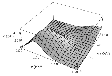
FIG. 6.: The total cross section of ¹²C + ¹²C $\rightarrow$ ²⁴Mg + $\pi^{0}$ as a function of the model parameters $v$ and $w$. The calculation is done for a pion momentum $41$ MeV/c which corresponds to the total energy of about $6$ MeV above threshold.

This figure indicates that a reasonable variation of parameters could cause a change in the answer by an order of magnitude. We emphasize again that in our calculations we did not project the participating nuclei onto appropriate shell-model states. Such a projection would require additional nuclear structure input. Given that the existing experimental data do not clearly resolve the structure of the final state this seems sufficient. As a conclusion, within all the limitations discussed above, the agreement between the introduced theory and the experimental results of this rare process seems to be remarkable.

D Calculations for heavy nuclei

In this section we apply the low-momentum approximation for the cross section described by Eq. (28) to several reactions, with the goal of understanding the general dependence with respect to the mass of the incoming nuclei. In order to calculate the cross section, one needs the harmonic oscillator parameter $v$ which can be estimated from the experimentally determined r.m.s. radii of the nuclei[20],

$$r_{\rm r.m.s.}^{2}={1\over A}\,\sum_{i}\left<r_{i}^{2}\right>=={1\over A}\,\sum_{i}\frac{1}{v^{2}}\left(\alpha_{i}+\frac{3}{2}\right).$$ (37)

In order to calculate the cross section, one needs to know the incoming energy of the nuclei as well as the energy of the outgoing pion. Calculations of the cross sections were performed for incoming nuclei ⁹Be, ¹²C, ¹⁶O and ²⁰Ne with corresponding fusion products ¹⁸O, ²⁴Mg, ³²S and ⁴⁰Ca in the limit of low pion momentum. In this limit the cross section is proportional to the cube of the pion momentum,

$$\sigma=\tilde{\sigma}(k^{3}/m_{\pi}^{3}).$$ (38)

Values of $\tilde{\sigma}$ are displayed as a function of the mass number of the incoming nuclei in Figure 7. The shell model configurations are again randomly chosen from the available set of Cartesian states that conserve isospin and parity. Average values are represented by filled diamonds while the states with the highest and lowest cross sections are represented by the boundaries of the error bars. The large error bars demonstrate the wide fluctuation in strengths for individual states. However, despite the fluctuations, it is clear that the overall trend is of a decreasing cross section with increasing mass.

Also shown in Figure 7 are experimental measurements represented by open circles for the $pp$, ³He³He and ¹²C¹²C cases discussed previously. The corresponding calculations, which were performed for the experimentally measured pion momenta rather than in the low-momentum limit are also displayed with closed circles. One sees that the cross sections fall by several orders of magnitude, but the measurements are still feasible throughout the wide range of masses. Calculations could be performed for heavier nuclei, but for larger masses the Coulomb barrier becomes important, and shuts off the possibility of fusion for masses larger than 20.

FIG. 7.: The general behavior of the pionic fusion cross section $A+A\,\rightarrow 2A+\pi$ versus the mass number of initial nucleus $A$. The plotted value $\tilde{\sigma}$ is related to a total cross section as $\sigma=\tilde{\sigma}\,(k/m_{\pi})^{3}$. Calculations in the low-momentum limit (filled diamonds) show that cross sections fall by several orders of magnitude in this mass range, but remain in the picobarn region for nuclei as large as oxygen. The highest and the lowest cross section found within the shell model configurations are represented by error bars. Experimental measurements are displayed (open circles) and compared to calculations (filled circles) which were performed for the finite pion momenta corresponding to the experiments.

VI Conclusions

Near threshold meson production represents a unique area of heavy ion reactions. In this area the reactions underline the pronounced features of quantum many-body physics. Most theoretical approaches to understanding and predicting these phenomena lose their validity in such an extreme regime. In this paper we have proposed a simple model to study the processes of deep subthreshold pion production. The pionic fusion cross section was obtained in a Born approximation with respect to pion production and in the sudden approximation for the nuclear rearrangement. The participating nuclei were described by the harmonic oscillator shell model in moving oscillator potentials. The advantage of the method is that it allows one to incorporate energy, momentum, spin and isospin conservation laws precisely and respect the Pauli principle at all steps of the calculation. Further aspects of nuclear structure could be additionally taken into account. At threshold energies these constraints pose the most powerful restriction on the reaction and cannot be ignored as is done in statistical and kinetic models which are reasonable at higher energy. The obvious disadvantage of the model is that the sudden approximation does not consider the slow changes of the nuclear mean field in the process of interaction. For the future developments it seems feasible to incorporate the time dependence and solve the equations for the evolution of a nuclear mean field parameters.

The nearly analytical form of overlaps greatly simplified the calculations for this study. We used a spherically symmetric nuclear mean field but in some cases this symmetry prohibits the transition and this would require a consideration of deformations, i.e. different oscillator parameters for different directions. The above mentioned limitations are reflected by the difficulty in determining the parameters of the model, and lead to about an order of magnitude ambiguity in the result for $s$-$d$ shell nuclei. More realistic single-particle wave functions could be incorporated into the model. Some of the exponential factors in Eqs. (19) and (23) arise directly from the Fourier transformation of the Gaussian tails in harmonic oscillator wave functions and could be substituted with modified factors that would reflect a more realistic behavior.

We would like to stress here again that pionic fusion is a very rare process presenting a tiny fraction of the total cross section. The agreement that was observed between calculations and experimental data for the cross sections ranging from $10^{-4}$ to $10^{-9}$ barns is remarkable. Within the limits of the low pion momentum approximation in the class of the reactions $A+A\rightarrow 2A+\pi$, we were able to obtain a general formula, Eq. (28), for the cross sections. The proposed techniques can certainly be applied in the same manner to other pion production reactions. The processes of electrofission [21] present an another interesting avenue to exercise this technique.

Appendix

A Harmonic oscillator wave functions and overlaps

Work with harmonic oscillator wave functions often involves integrations of the expressions constructed of polynomials and Gaussian weights. Thus, the following integral is useful $(a>0)$,

$$\int_{\infty}^{+\infty}x^{n}e^{-ax^{2}+ibx}\,dx=\sqrt{\pi\over a}e^{-b^{2}/4a}\quad a^{-n/2}\,T_{n}\left({ib\over{2\sqrt{a}}}\right)\quad,$$ (39)

where $T_{n}(x)$ is a sum arising from the binomial expansion,

$$T_{n}(x)=\sum_{j=0,2,4\ldots}^{n}{n!(j-1)!!\over j!(n-j)!2^{j/2}}x^{n-j}\quad.$$ (40)

This expression can be used for the evaluation of any integral encountered in this work. There are two important limiting cases for the sum $T_{n}(x)$, $x\rightarrow 0$ and $x\gg 1$:

$$\lim_{x\rightarrow 0}T_{n}(x)=\left\{\matrix{{(n-1)!!\over 2^{n/2}}\quad{\rm if}\;n\;{\rm is\;even}\cr 0\quad{\rm if}\;n\;{\rm is\;odd}}\right.\quad,\quad\lim_{x\rightarrow\infty}T_{n}(x)=2^{-n/2}\,x^{n}\quad.$$ (41)

The Gaussian-Fourier integration of Eq. (39) is a transformation on the space of polynomials defined on the basis

$$x^{n}\rightarrow[x^{n}](p)=T_{n}(p)$$ (42)

The following two-dimensional integrals often appear in our calculations,

$$\int\int(x-y)^{n}e^{-a(x^{2}+y^{2})}dx\,dy=\left\{\matrix{\pi a^{-1-n/2}(n-1)!!\quad{\rm if}\;n\;{\rm is\;even}\cr 0\quad{\rm if}\;n\;{\rm is\;odd}}\right.\quad,$$ (43)

$$\int\int(x-y)^{n}e^{-a(x^{2}+y^{2})}e^{ip(x-y)}dx\,dy={\pi\over a}\left({2\over a}\right)^{n/2}e^{-p^{2}/2a}T_{n}\left({ip\over\sqrt{2a}}\right)\quad.$$ (44)

The basic block of the calculations is the overlap of two one-dimensional harmonic oscillator wave functions with different oscillator parameters, shifted locations of the centers and possible additional factor $e^{-ikx}$ that enters the single-particle interaction integral from Eq.(5). This type of integral, the generalized Debye-Waller factor, can be written in a factorized form:

$$\langle(\beta;r)_{v}|e^{-ikx}|(\alpha;r^{\,\prime})_{w}\rangle=\eta^{1/2}\times$$ (45)

$$\exp\left({\frac{-k^{2}}{2(v^{2}+w^{2})}-\frac{(r-r^{\,\prime})^{2}v^{2}w^{2}}{2(v^{2}+w^{2})}-{\frac{ik(rv^{2}+r^{\,\prime}w^{2})}{(v^{2}+w^{2})}}}\right)P_{\beta\,\alpha}((r^{\,\prime}-r),k;v,w)\,,$$ (46)

where $\eta$ is given by Eq. (21) and $P_{n\,m}(r,k;v,w)$ is a dimensionless polynomial of $r$ and $k$ of the highest power $n+m$ with coefficients dependent on $w$ and $v$. The following are examples of these polynomials for the smallest values of $n$ and $m$:

$$P_{0\,0}(r,k;v,w)=1\,,$$ (47)

$$P_{0\,1}(r,k;v,w)=P_{1\,0}(-r,k;w,v)=-{\frac{{\sqrt{2}}\,\left(i\,k+r\,{v^{2}}\right)\,w}{{v^{2}}+{w^{2}}}}\,,$$ (48)

$$P_{1\,1}(r,k;v,w)={\frac{2\,v\,w\,\left({v^{2}}+{w^{2}}-\left(k-i\,r\,{v^{2}}\right)\,\left(k+i\,r\,{w^{2}}\right)\right)}{{{\left({v^{2}}+{w^{2}}\right)}^{2}}}}\,.$$ (49)

The technique of obtaining these expressions is simple though tedious. An important situation $k=0$ would correspond to the overlap of two wave functions without a pion production, in this case we will not write $k$ as an argument. It can be shown that [19]

$$P_{i\,j}(r;v,w)=\sum_{k+l=0,2,4\ldots}^{k=i,l=j}{\sqrt{{\frac{i!\,j!}{k!\,l!}}}}\,{\frac{{{\left(-1\right)}^{j-l}}\,{v^{j-l}}\,{w^{i-k}}}{\left(i-k\right)!\,\left(j-l\right)!}}\,{{\left({\frac{r\,\eta}{\sqrt{2}}}\right)}^{i+j-k-l}}P_{k\,l}(0;v,w)$$ (50)

and

$$P_{k\,l}(0;v,w)=\sqrt{k!\over l!}{\cal P}_{{(k+l)/2}}^{{(l-k)/2}}\left(\eta\right)\quad,$$ (51)

with ${\cal P}_{\alpha}^{\beta}$ being the associated Legendre polynomials. A bit simpler case is

$$P_{i\,j}(r;v=w=1)=\sqrt{{i!j!\over 2^{i+j}}}(-1)^{j}\sum_{k=0}^{min(i,j)}(-1)^{k}r^{i+j-2k}{2^{k}\over k!(i-k)!(j-k)!}\quad.$$ (52)

Any three-dimensional overlap is reduced to the one-dimensional form of Eq. (46) in a direct way

$$\langle({\vec{\beta}};{\bf R})|({\vec{\alpha}};{\bf r})\rangle=\prod_{x=1,2,3}\langle(\beta_{x};R_{x})|(\alpha_{x};r_{x})\rangle\quad.$$ (53)

Similarly we introduce

$$\langle({\vec{\beta}},{\bf r})|e^{-i{\bf k}\cdot{\bf x}}|({\vec{\alpha}},{\bf r}^{\,\prime})\rangle=\eta^{3/2}\times$$ (54)

$$\exp\left({\frac{-k^{2}}{2(v^{2}+w^{2})}-\frac{({\bf r}-{\bf r}^{\,\prime})^{2}v^{2}w^{2}}{2(v^{2}+w^{2})}-\frac{-i{\bf k}({\bf r}v^{2}+{\bf r}^{\,\prime}w^{2})}{(v^{2}+w^{2})}}\right)P_{{\vec{\beta}}\,{\vec{\alpha}}}(({\bf r}^{\,\prime}-{\bf r}),{\bf k};v,w)\quad,$$ (55)

where

$$P_{{\vec{\beta}}\,{\vec{\alpha}}}(({\bf r}^{\,\prime}-{\bf r}),{\bf k};v,w)=\prod_{x=1,2,3}P_{\beta_{x}\,\alpha_{x}}(r^{\,\prime}_{x}-r_{x},k_{x};v,w)\quad.$$ (56)

B Calculational details of the $A+A\rightarrow 2A+\pi^{+}$ reaction.

Overlaps of many-body nucleon wave functions can be expressed in our approximation by a determinant of single-particle overlaps:

$$\langle({\vec{\beta}}_{1},\ldots,{\vec{\beta}}_{n};{\bf R})|({\vec{\alpha}}_{1},\ldots;{\bf r})(\ldots;{\bf r}^{\,\prime})\rangle\,=\left|\matrix{\langle({\vec{\beta}}_{1};{\bf R})|({\vec{\alpha}}_{1};{\bf r})\rangle&\cdots&\langle({\vec{\beta}}_{1};{\bf R})|({\vec{\alpha}}_{n};{\bf r}^{\,\prime})\rangle\cr\vdots&\ddots&\vdots\cr\langle({\vec{\beta}}_{n};{\bf R})|({\vec{\alpha}}_{1};{\bf r})\rangle&\cdots&\langle({\vec{\beta}}_{n};{\bf R})|({\vec{\alpha}}_{n};{\bf r}^{\,\prime})\rangle\cr}\right|\,.$$ (57)

Eq. (55) allows one to take identical exponential multipliers in each row outside the determinant as a common factor in all calculations leaving only the matrix of polynomials $P_{{\vec{\beta}}\,{\vec{\alpha}}}$ to be evaluated. A simple example of this is the calculation of the normalization:

$$\langle({\vec{\alpha}}_{1},{\vec{\alpha}}_{2}\ldots{\vec{\alpha}}_{A};{\bf r})_{v})|({\vec{\alpha}}_{1},{\vec{\alpha}}_{2}\ldots{\vec{\alpha}}_{A};{\bf r}^{\,\prime})_{v}\rangle=||P({\bf r}-{\bf r}^{\,\prime};v,v)||e^{-A({\bf r}-{\bf r}^{\,\prime})^{2}v^{2}/4}\,e^{i{\bf p}({\bf r}-{\bf r}^{\,\prime})}\,.$$ (58)

In this expression $||P({\bf r}-{\bf r}^{\,\prime};v,v)||$ is a determinant of a matrix with the entries $P_{{\vec{\alpha}}_{i}\,{\vec{\alpha}}_{j}}$. As discussed in Sect II, this overlap is equal to that of the CM wave functions of two harmonic oscillators located at ${\bf r}$ and ${\bf r}^{\,\prime}$. For a nucleon system in the lowest state (in terms of harmonic oscillator shell excitations), the CM wave function is the harmonic oscillator wave function of the ground state $|(0,{\bf r})_{\varsigma}\rangle$. We obtain an interesting mathematical fact

$$||P({\bf r}-{\bf r}^{\,\prime};v,v)||=P_{0\,0}({\bf r}-{\bf r}^{\,\prime};\varsigma,\varsigma)=1\,.$$ (59)

Comparison of the exponents in Eq. (58) and Eq. (55) gives the value of the oscillator parameter for the center-of-mass oscillation as $\varsigma=v\sqrt{A}$.

With the same strategy, one can approach the calculation of the reaction $A+A\rightarrow 2A+\pi^{+}$ extracting all exponential factors. Corresponding values of the overlaps $F_{n}$,$G_{l}$ and $H_{n\,l}$ may be rewritten, defining new polynomials $f_{n}$, $g_{l}$ and $h_{n\,l}$:

$$F_{n}=\eta^{3(2Z-1)/2}\times\left\{\matrix{\exp\left(-{\eta vw}\left[Z({\bf R}-{\bf r})^{2}+(Z-1)({\bf R}-{\bf r}^{\,\prime})^{2}\right]/4\right)\,f_{n}&n\leq Z\,,\cr\exp\left(-{\eta vw}\left[(Z-1)({\bf R}-{\bf r})^{2}+Z({\bf R}-{\bf r}^{\,\prime})^{2}\right]/4\right)\,f_{n}&n>Z\,;}\right.$$ (60)

$$G_{l}=\eta^{3(2N)/2}\exp\left({-N{\eta vw}\left[({\bf R}-{\bf r})^{2}+({\bf R}-{\bf r}^{\,\prime})^{2}\right]/4}\right)\,g_{l}\,,$$ (61)

$$H_{nl}=\eta^{3/2}\exp\left(-{({{\bf R}-{\bf r}})^{2}v^{2}w^{2}+{\bf k}^{2}+2i{\bf k}\cdot({\bf R}v^{2}+{\bf r}w^{2})\over 2(v^{2}+w^{2})}\right)\,h_{nl}\qquad({\rm if}\,n>Z,\,r\Leftrightarrow r^{\,\prime})\,.$$ (62)

It is useful to notice here that all the polynomials are functions of distances between the nuclei $({\bf r}-{\bf R})$ and $({\bf r}^{\,\prime}-{\bf R})$ that we will denote as ${\bf x}$ and ${\bf y}$ respectively. Considering integration in Eq. (18) over variables ${\bf x}$, ${\bf y}$ and ${\bf R}$ we observe from Eq. (60) that the oscillating phase has the form

$$\exp\left({-i{\bf k}\cdot({\bf R}v^{2}+{\bf r}w^{2})\over(v^{2}+w^{2})}+i{\bf p}({\bf r}-{\bf r}^{\,\prime})-i{\bf p}_{f}\cdot{\bf R}\right)$$

$$=\exp\left({i{\bf p}\cdot({\bf x}-{\bf y})-{i{\bf k}\cdot{\bf x}w^{2}\over v^{2}+w^{2}}-i({\bf k}+{\bf p}_{f})\cdot{\bf R}}\right)\,,$$

and integration over ${\bf R}$ gives a momentum preserving $\delta$-function that requires ${\bf k}=-{\bf p}_{f}$. For convenience we split the sum in Eq. (18) over $n\leq Z$ and $Z<n\leq 2Z$ and substitute $F$, $G$ and $H$ from Eq. (60)

$$\langle F|H|I\rangle={1\over{\cal N}_{i}{\cal N}_{f}}\int{V\over{\sqrt{2\omega V}}}{1\over 2m}\eta^{3A}\,e^{-Avw\eta(x^{2}+y^{2})/4}\,e^{-k^{2}/2(v^{2}+w^{2})}$$ (63)

$$=\left(e^{-i{\bf k}\cdot{\bf x}\eta w/2v}\sum_{i\leq Z,\,j}(-1)^{i+j}f_{i}g_{j}h_{ij}+e^{-i{\bf k}\cdot{\bf y}\eta w/2v}\sum_{i>Z,\,j}(-1)^{i+j}f_{i}g_{j}h_{ij}\right)e^{-i{\bf p}\cdot({\bf x}-{\bf y})}d^{3}xd^{3}y\,.$$ (64)

The terms $\sum f_{i}g_{j}h_{ij}$ are again some polynomials of ${\bf x}$ and ${\bf y}$ proportional to $|k|$ and containing parameters $v$ and $w$. The final integration can be performed with the help of Eq. (39) corresponding parameters $a$ and $b$ being

$$a=A\eta vw/4\quad,\quad b=\pm\,p-k\eta w/2v\quad.$$ (65)

As a result, we arrive at the formula (19) with polynomials

$$P(k,p)={1\over|{\bf k}|}\left[\sum_{i\leq Z,\,j}(-1)^{i+j}f_{i}g_{j}h_{ij}\right]\left(-i\,{{\bf p}+{\bf k}\eta w/2v\over\sqrt{A\eta vw}}\,,\,{i{\bf p}\over\sqrt{A\eta vw}}\right)\,,$$ (66)

$$Q(k,p)={1\over|{\bf k}|}\left[\sum_{i>Z,\,j}(-1)^{i+j}f_{i}g_{j}h_{ij}\right]\left({-i{\bf p}\over\sqrt{A\eta vw}}\,,\,i\,{{\bf p}-{\bf k}\eta w/2v\over\sqrt{A\eta vw}}\right)\,,$$ (67)

where the first argument is the transformation of elements of vector ${\bf x}$ and the second that of vector ${\bf y}$. From here it is also seen that if before transformation there existed a symmetry between ${\bf x}$ and ${\bf y}$, i.e. the nuclei were in an identical state, then $P({\bf k},-{\bf p})=Q({\bf k},{\bf p})$.

C Toward a complete analytical answer, reaction $A+A\rightarrow 2A+\pi^{0}$.

As it was pointed out in the main text, the amplitude of the pionic process is approximately proportional to the amplitude of the fusion reaction. One can study the properties of the determinants arising in a fusion reaction in a quite general way, separately considering the four types of particles distinguished by spin and isospin in the reaction of fusion of the type $A+A\rightarrow 2A$. This leads to the following form of a single-particle overlap matrix

$$2A\left\{\left(\matrix{\langle({\vec{\beta}}_{1};{\bf R})|({\vec{\alpha}}_{1};{\bf r})\rangle\cdots&&\cdots\langle({\vec{\beta}}_{1};{\bf R})|({\vec{\alpha}}_{A};{\bf r}^{\,\prime})\rangle\cr\vdots&&\vdots\cr\underbrace{\langle({\vec{\beta}}_{A};{\bf R})|({\vec{\alpha}}_{1};{\bf r})\rangle\cdots}_{{\rm first}\,A\,{\rm nucleons}}&&\underbrace{\cdots\langle({\vec{\beta}}_{A};{\bf R})|({\vec{\alpha}}_{A};{\bf r}^{\,\prime})\rangle}_{{\rm second}\,A\,{\rm nucleons}}\cr}\right)\right.\,.$$ (68)

Without loss of generality, ${\bf R}$ can be set to zero. A second important feature is that in nuclei under consideration all inner shells are filled. Therefore, the resulting determinant is a function of a nucleon number $A$ and extra parameters arising from different ways to distribute the particles in the outer shells.

It is interesting to present the exact result for the one-dimensional case where the problem is uniquely defined. We consider two oscillators with single-particle states from $0$ till $A-1$ overlapping with one larger oscillator with occupied states from $0$ up to $2A-1$,

$$\left|\matrix{\langle(0;0)_{v}|(0;x)_{w}\rangle&\cdots&\langle(0;0)_{v}|(A-1;y)_{w}\rangle\cr\vdots&\ddots&\vdots\cr\langle(2A-1;0)_{v}|(0;x)_{w}\rangle&\cdots&\langle(2A-1;0)_{v}|(A-1;y)_{w}\rangle\cr}\right|$$ (69)

$$={\frac{{(-1)^{A}(w(x-y))^{A^{2}}\sqrt{\left(2\,A\right)!}}}{{2^{{\frac{\left(A-1\right)\,A}{2}}}}\,{\sqrt{A!}}\,\left(\prod_{i=1}^{A}{\frac{\left(2\,i\right)!}{i!}}\right)}}\,\eta^{(2A-1)A}={1\over\gamma}(w(x-y))^{q}\,\eta^{\cal Q}\quad,$$ (70)

$$\gamma(A)={(-1)^{A}\,\sqrt{A!}\over\sqrt{(2A)!}}{{2^{{\left(A-1\right)\,A}/{2}}}\,\left(\prod_{i=1}^{A}{\frac{\left(2\,i\right)!}{i!}}\right)}\,.$$ (71)

The result is just a single term which depends only on the distance between the two initial oscillator locations raised to the power equal to the difference in total number of quanta between initial and final systems, $q=A^{2}$. The term $\eta=2vw/(v^{2}+w^{2})$ comes in the power of total number of quanta in the final nucleus, ${\cal Q}=(2A-1)A$. This remains true only for Fermi systems in the ground state, i.e. if there are no gaps in the harmonic oscillator single-particle level occupation. The situation for a three-dimensional oscillator is similar. The required polynomial is still given by one term that has a form of the product

$${1\over\gamma}(x_{x}-y_{x})^{q_{x}}(x_{y}-y_{y})^{q_{y}}(x_{z}-y_{z})^{q_{z}}w^{q_{x}+q_{y}+q_{z}}\,\eta^{{\cal Q}_{f}}\quad,$$ (72)

where integers $q_{x}$, $q_{y}$ and $q_{z}$ are differences of the number of quanta between the final and initial systems in $x$, $y$ and $z$ directions, respectively. A specific three-dimensional complication arises from the following aspect. The lowest energy state is, in general, degenerate as for non-magic nuclei one has the freedom of placing several particles into $(n+1)(n+2)/2$ degenerate levels of the $n$-th shell. The numerical parameter $\gamma$ depends in this case also on the way the particles are placed in the outer shell of each nucleus. The harmonic oscillator symmetries in the problem often prohibit the transition.

The polynomials in Eq. (64) acquire a form of a product of four components, each of the form of Eq. (72) for each type of nucleons, times the sum of terms $({\vec{\sigma}}\cdot{\bf k})$ acting on every pair of interacting nucleon species. Using the integrals from Eq. (43) and writing the action of $({\vec{\sigma}}\cdot{\bf k})$ between initial and final spin parts of the wave function as a matrix element ${\tilde{M}}$ we arrive at the expression for the polynomial in Eq. (24)

$$P_{q_{x},q_{y},q_{z}}(k=0,p)={1\over\gamma}\left({2(v^{2}+w^{2})\over Av^{2}}\right)^{(q_{x}+q_{y}+q_{z})/2}\,\eta^{{\cal Q}_{f}}\times$$ (73)

$$\left((q_{x}-1)!!\,(q_{y}-1)!!\,2^{q_{z}\over 2}T_{q_{z}}\left({ip\sqrt{2\over A\eta vw}}\right)\right){\tilde{M}}\quad.$$ (74)

In the above expression we have redefined $\gamma$ as a product of $\gamma$’s for all four types of nucleons.

REFERENCES

- [1] D. Horn et al., Phys. Rev. Lett. 77, 2408 (1996).
- [2] Y. Le Bornec et al., Phys. Rev. Lett. 47, 1870 (1981).
- [3] M. Waters et al., Nucl. Phys. A564, 595 (1993).
- [4] J. Miller et al., Phys. Rev. Lett. 58, 2408 (1987).
- [5] B. Erazmus et al., Phys. Rev. C44, 1212 (1991).
- [6] P. Braun-Munzinger, P. Paul, L. Ricken, J. Stachel, P. H. Zhang, G. R. Young, F. E. Obenshain and E. Grosse, Phys. Rev. Lett. 52, 255 (1984).
- [7] T. Suzaki, et al., Phys. Lett. B257, 27 (1991).
- [8] D. Vasak, H. Stöcker, B. Müller and W. Greiner, Phys. Lett. 93b, 243 (1980).
- [9] D. Vasak, B. Müller and W. Greiner, J. Phys. G: Nucl. Phys. 11, 1309 (1985).
- [10] G. Li, D. T. Khoa, T. Maruyama, S. W. Huang, N. Ohtsuka and A. Faessler, Nucl. Phys A534, 697 (1991).
- [11] A. Bonasera, G. Russo and H. H. Wolter, Phys. Lett. B 246, 337 (1990).
- [12] C. Providência and D. Brink, Nucl. Phys. A485, 699 (1988).
- [13] D. S. Koltun and A. Reitan, Phys. Rev. 141, (1966) 1413.
- [14] T. Sato, T.-S. H. Lee, F. Myhrer, and K. Kubodera, Phys. Rev. C56, 1246 (1997).
- [15] T. Ericson and W. Weise, Pions and Nuclei (Clarendon Press, Oxford, 1988).
- [16] E. K. Warburton and D. J. Millener, Phys. Rev. C 39, 1120 (1989).
- [17] S. Karataglidis, P. Halse, and K. Amos, Phys. Rev. C 51, 2494 (1995).
- [18] S. Karataglidis, P. J. Dortmans, K. Amos and R. de Swiniarski, Phys. Rev C 52, 861 (1995).
- [19] A. I. Baz, I. B. Zeldovich and A. M. Perelomov, Scattering, reactions and decay in nonrelativistic quantum mechanics (Jerusalem, Israel Program for Scientific Translations, 1969).
- [20] H. De Vries et al., Atomic Data and Nuclear Data Tables, Vol 36, No. 3 (1987).
- [21] A. M. Sandorfi, J. R. Calarco, R. E. Rand and H. A. Schwettman, Phys. Rev. Lett. 45, 1615 (1980).