THREE NUCLEONS AT VERY LOW ENERGY

Abstract

We discuss the effective field theory approach to nuclear phenomena with typical momentum below the pion mass. We particularly focus on the three body problem. In the $J=3/2$ channel, effective field theory is extremelly predictive and we are able to describe the nucleon-deuteron scattering amplitude at the percent level using only two parameters obtained from nucleon-nucleon scattering. We briefly comment on the $J=1/2$ channel and the issues related to the non-perturbative renormalization of the three body force.

1 Introduction

Most of the early work on the use of effective field theory in nuclear physics concentrated on the momentum scale $p\sim m_{\pi}$. There is a good reason for that: most of nuclear phenomenology is at this scale (the Fermi momentum in nuclear matter, for instance, is at the order of $2m_{\pi}$). This talk, however, will concentrate on the scale $p\sim 1/a\ll m_{\pi}$ ($a$ is the nucleon-nucleon scattering lenght), that will be refered to as the “ very low ” momentum scale. This scale region is interesting for three reasons. The first reason is that this scale, even though not typical in nuclei, is relevant for a corner of nuclear physics. This comes about because the deuteron is an anomalously shallow bound state, with a binding energy of the order of $1/Ma^{2}$, what sets the momentum scale of deuteron physics to be $p\sim 1/a\ll m_{\pi}$. A second reason is that, since pions can be integrated out and don’t appear as explicit degrees of freedom, a number of issues related to regularization and renormalization, many of them extensively discussed in this workshop, can be addresed in a simpler situation. The third motivation to consider the “ very low ” momentum scale is related to recent work on the “ low ” momentum scale $p\sim m_{\pi}$ . At this higher momentum scale pions have to be included explicitly and in previous power counting schemes the whole ladder of pion exchanges contributed at leading order to nucleon-nucleon scattering. This is a source of tremendous complication, both conceptual and practical. Recently a new power counting scheme was suggested [1],[2] in which pion exchanges are perturbative and, in particular, the leading order contains no pion exchanges. Thus, all results obtained discussed here using the effective theory appropriate to the $p\ll m_{\pi}$ scale will automatically equal the leading order result obtained from this new power counting of valid at the $p\sim m_{\pi}$ scale.

In the absence of explicit pions, the effective theory method applied to nucleon-nucleon scattering simply reproduces the effective range expansion. This is phenomenologically correct, but hardly interesting. The first nontrivial application is the three body problem, that is the main subject of this talk.

2 The very low energy effective theory

For momenta much smaller than the pion mass, the only degrees of freedom that need to be included explicitly are the nucleons. The effect of pion exchanges, $\Delta$’s, heavier meson, etc., are all implicitly included in the coefficient of local operators in the lagrangean. We will concentrate later on the three body problem in the $J=3/2$ channel. In this channel all nucleon spins are parallel thus all s-wave two nucleon interactions are in the spin triplet channel. Restricting ourselves to spin triplet interactions, the most general lagrangean is :

$${\cal L} = N^{\dagger}(i\partial_{0}+\frac{\vec{\nabla}^{2}}{2M}+\ldots)N+C_{0}(N^{\dagger}\tau_{2}\vec{\sigma}\sigma_{2}N)^{2}$$ (1)

$$+C_{2}\left[(N^{\dagger}\tau_{2}\vec{\sigma}\sigma_{2}\nabla N)(N^{\dagger}\tau_{2}\vec{\sigma}\sigma_{2}\nabla N)-3(N^{\dagger}\tau_{2}\vec{\sigma}\sigma_{2}N)(N^{\dagger}\tau_{2}\vec{\sigma}\sigma_{2}\nabla^{2}N)+h.c.\right]$$

$$+\ldots,$$

where $M$ is the nucleon mass, $C_{n}$ are constants related to the two-body force terms containing $n$ derivatives, and the dots stand for higher-order terms including relativistic corrections, higher-derivative terms, three-body forces, etc. Terms describing the spin singlet interactions have a similar form but will not be needed here. The constants $C_{n}$ are determined by nucleon-nucleon scattering data. As it was explained in more detail in van Kolck’s [3] talk it turns out that, using dimensional regularization and minimal subtraction, $C_{0}\sim a/M$, $C_{2}\sim r_{0}(r_{0}a)/M$, $C_{4}\sim r_{0}(r_{0}a)^{2}/M+\ldots$ and so on ($r_{0}$ is the effective range and ellipses stand for terms suppressed by powers of $r_{0}/a$ ). The leading pieces in each one of these terms form a geometric series that can be conveniently summed to all orders by the introduction of a field of baryon-number two [5]

$$\cal L = N^{\dagger}(i\partial_{0}+\frac{\vec{\nabla}^{2}}{2M}+\ldots)N+\vec{d}^{\dagger}\cdot(-i\partial_{0}-\frac{\vec{\nabla}^{2}}{4M}+\Delta+\ldots)\vec{d}$$ (2)

$$-\frac{g}{2}(\vec{d}^{\dagger}\cdot N\vec{\sigma}\sigma_{2}\tau_{2}N+\mbox{h.c.})+\ldots$$

If the dibaryon field $\vec{d}$ is integrated out, the Lagrangian (1) is recovered as long as $\Delta$ and $g$ are appropriate functions of $C_{0}$ and $C_{2}$. This resummation is by no means necessary, since for momenta of the order $p\sim 1/a$ the resummed terms are subleading, but it is just a convenient way of computing higher-order corrections.

The numerical values of $g$ and $\Delta$ can be determined if we consider the dressed dibaryon propagator (Fig. 1).

Figure 1: Dressed dibaryon propagator.

The linearly divergent loop integral is set to zero in dimensional regularization and the result is

$$iS(p)=\frac{1}{p^{0}-\frac{\vec{p}^{\,2}}{4M}-\Delta+\frac{Mg^{2}}{2\pi}\sqrt{-Mp^{0}+\frac{\vec{p}^{\,2}}{4}-i\epsilon}+i\epsilon}.$$ (3)

This propagator is, up to a constant, the scattering matrix of two nucleons in the ${}^{3}S_{1}$ channel,

$$T(k)={4\pi\over M}{1\over-\frac{2\pi\Delta}{Mg^{2}}+\frac{2\pi}{M^{2}g^{2}}k^{2}-ik},$$ (4)

where $k^{2}/M$ is the energy in the center-of-mass frame. This result is just the familiar effective range expansion, from what we can infer the proper values for the constants $g$ and $\Delta$. Using $a=5.42$ fm and $r_{0}=1.75$ fm [7], we find

$$g^{2} =\frac{4\pi}{M^{2}r_{0}} =1.6\cdot 10^{-3}\ {\rm MeV^{-1}},$$ (5)

$$\Delta =\frac{2}{Mar_{0}} =8.7\ {\rm MeV}.$$ (6)

From Eqs. (3), (5), and (6) we see why it is necessary to resum the bubble graphs in Fig. 1 to all orders for $p\sim 1/a$: the term in the square root coming from the unitarity cut is of the same order as $\Delta$. On the other hand, as mentioned before, the kinetic term of the dibaryon is smaller than the other terms in (3) and is resummed for convenience only. Notice that the propagator (3) has two poles, one at $p^{0}=\vec{p}^{\,2}/4M-B$ (the deuteron pole), another at $p^{0}=\vec{p}^{\,2}/4M-B_{deep}$ (unphysical deep pole), and a cut along the positive real axis starting at $p^{0}=\vec{p}^{\,2}/4M$.

3 Power counting for neutron-deuteron scattering

Let us now turn to neutron-deuteron scattering. We want to identify which graphs give the leading contributions in an expansion on powers of the typical momentum $p\sim 1/a$ over the scale of the physics not explicitly included in the effective theory $m_{\pi}\sim 1/r_{0}$.

The simplest diagram contributing to neutron-deuteron scattering is the first diagram on the right hand side of Fig. 2.

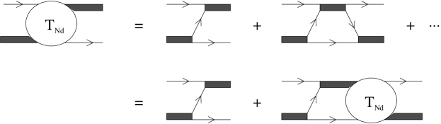
Figure 2: Dressed dibaryon propagator.

For momenta of the order of $p\sim 1/a$ it gives a contribution of the order of $g^{2}/(p^{2}/M)\sim a^{2}/Mr_{0}$. The one-loop graph mixes different orders of the expansion, since it involves the dibaryon propagator $g^{2}/(\Delta+p^{2}/M)\sim(a/M)(1+{\cal O}(r_{0}/a)+\ldots)$. It also involves a loop. The contribution coming from loops can be estimated by rescaling all internal energies by $p^{2}/M$, ,where $p$ is some typical external momentum. The result is $\sim M^{n}p^{m}$, where $n=$number of nucleons propagators minus the number of loops and $m$ can be determined by dimensional analysis. Using this rule we can easily estimate the one loop graph in Fig. 2 to be $g^{2}g^{2}/(\Delta+p^{2}/M)\sim(a^{2}/Mr_{0})(1+{\cal O}(r_{0}/a)+\ldots)$. Similarly we can see that the remaining graphs in Fig. 2 give contributions of the same order, which means that an infinite number of diagrams contribute to the leading orders.

Other contributions are suppressed by at least three powers of $r_{0}/a$ or $pr_{0}$. For instance, the effect of the subleading (not resummed) piece of $C_{4}$ is to generate the shape parameter ($\sim k^{4}$) term in the effective range expansion of the nucleon-nucleon interaction. Its typical size is $\sim k^{4}r_{0}^{3}$ compared to the leading piece $\sim 1/a$ and is thus also suppressed by $(r_{0}/a)^{3}$. Likewise, p-wave interactions, unaffected by the existence of a shallow s-wave bound state, arise from a term in the lagrangean with two derivatives and a coefficient of the order $\sim 1/Mm_{\pi}^{3}$. We conclude then that a diagram made out of the substitution of one of the dibaryon propagators in a diagram in Fig. 2 by a p-wave interaction vertex would be suppressed by $(r_{0}/a)^{3}$ in comparison to the leading order. Three-body force terms have to contain at least two derivatives since in the $J=3/2$ channel all the spins are up and Fermi statistics forbids the placement of all three nucleon in a s-wave. The natural size of the coefficient of the six nucleon, two derivative term is $1/Mm_{\pi}^{6}$. A diagram including this three body force includes two nucleon loops, each one giving a $Mp$ factor, two dibaryon-two nucleons vertices and a three body force vertex, for a total contribution of the order of $p^{4}/Mm_{\pi}^{6}r_{0}\sim a^{2}/Mr_{0}(r_{0}/a)^{6}$. Thus contributions coming from the three-body force are suppressed in relation to the leading order graphs by $(r_{0}/a)^{6}$.

4 Summing the leading graphs

From the results of the previous section we see that a calculation accurate up to corrections of order $(r_{0}/a)^{3}$ is possible by summing the diagrams of Fig. 2. Fortunately, the interaction mediated by the s-channel dibaryon generates a very simple, local and separable potential between nucleons. It is well known that the three-body problem with separable two-body interactions reduces to an equivalent two-body problem. In our case the equation to be solved can be read off Fig. 2, and an integration over the energy inside the loop gives [4]

$$\tilde{t}(\vec{p},\vec{k})= - \frac{1}{(\vec{p}-\vec{k}/2)^{2}+MB}$$

$$- \int\frac{d^{3}l}{(2\pi)^{3}}\frac{\tilde{t}(\vec{l},\vec{k})}{-\frac{3(\vec{l}^{\,2}-\vec{k}^{2})}{8M^{2}g^{2}}+\frac{1}{4\pi}({\sqrt{\frac{3}{4}(\vec{l}^{\,2}-\vec{k}^{2})+MB}-\sqrt{MB}})}$$

$$\phantom{\int\frac{d^{3}l}{(2\pi)^{3}}}\frac{1}{\vec{l}^{2}-\vec{l}\cdot\vec{p}+\vec{p}^{\,2}-\frac{3}{4}\vec{k}^{2}+MB},$$

where $B$ is the deuteron binding energy and $\tilde{t}$ is a correlator with two dibaryon and two nucleons external legs represented by the blob in 2. One could have computed the deuteron-nucleon amplitude from the correlator involving any other operator with the deuteron quantum numbers instead of the dibaryon used here. The results for the (on shell) deuteron-nucleon scattering are obviously independent of this choice as long as the proper wave function renormalization is performed. The scattering matrix is given by

$$t(p)=\sqrt{Z}\ \tilde{t}(p,p)\ \sqrt{Z},$$ (8)

where $Z$ is defined by

$$Z=iS_{0}(p)|_{\rm pole}/iS(p)|_{\rm pole}=-\frac{1}{1-\frac{M^{2}g^{2}}{4\pi\sqrt{MB}}}.$$ (9)

It is convenient then to define the off-shell scattering amplitude

$$t(p,k)=\frac{\vec{p}^{\,2}-\vec{k}^{2}}{-\frac{3(\vec{p}^{\,2}-\vec{k}^{2})}{8M^{2}g^{2}}+\frac{1}{4\pi}({\sqrt{\frac{3}{4}(\vec{p}^{\,2}-\vec{k}^{2})+MB}-\sqrt{MB}})}\tilde{t}(p,k),$$ (10)

satisfying

$$\left[-\frac{3(\vec{p}^{\,2}-\vec{k}^{2})}{8M^{2}g^{2}}+\frac{1}{4\pi}({\sqrt{\frac{3}{4}(\vec{p}^{\,2}-\vec{k}^{2})+MB}-\sqrt{MB}})\right]\frac{t(\vec{p},\vec{k})}{\vec{p}^{\,2}-\vec{k}^{2}-i\epsilon}$$

$$=\frac{-1}{(\vec{p}-\vec{k}/2)^{2}+MB}-\int\frac{d^{3}l}{(2\pi)^{3}}\frac{1}{\vec{l}^{2}-\vec{l}\cdot\vec{p}+\vec{p}^{\,2}-\frac{3}{4}\vec{k}^{2}+MB}\frac{t(\vec{l},\vec{k})}{\vec{l}^{2}-\vec{k}^{\,2}-i\epsilon},$$

that reduces to the scattering amplitude $t(p)$ on shell

$$t(p)=t(p,p).$$ (12)

Since we are interested only in s-wave scattering, we should project this equation into its $L=0$ component. The result is

$$\frac{3}{2}\left[-\eta+\frac{1}{\sqrt{\frac{3}{4}(x^{2}-y^{2})+1}+1}\right]a(x,y)=-\frac{1}{xy}{\rm ln}\left(\frac{(x+y/2)^{2}+1}{(x-y/2)^{2}+1}\right)$$ (13)

$$-\frac{2}{\pi x}\int_{0}^{\infty}\ dz\ z{\rm ln}\left(\frac{z^{2}+x^{2}+1-\frac{3}{4}y^{2}+xz}{z^{2}+x^{2}+1-\frac{3}{4}y^{2}-xz}\right)\frac{a(z,y)}{z^{2}-y^{2}-i\epsilon},$$

where we use the dimensionless quantities $x=p/\sqrt{MB}$, $y=k/\sqrt{MB}$, $z=l/\sqrt{MB}$, and $a(x,y)=\frac{\sqrt{MB}}{4\pi}t_{L=0}(p,k)$, and $\eta=\sqrt{MB}r_{0}/2$. For finite values of $k$ this equation is complex even below threshold ($3k^{2}/4=B$) due to the $i\epsilon$ prescription. The numerical solution of the equation above is trivial in terms of computer power. The only subtle point is how to deal with the $i\epsilon$ prescription that appears in eq.(13). One way of dealing with that is to use the real $K$-matrix defined by

$$K(x,y)=\frac{a(x,y)}{1+iya(y,y)},$$ (14)

which satisfies the equation

$$K(x,y)=-h(x,y,y)-\frac{2}{\pi}\int_{0}^{\infty}\ dz\ z^{2}h(x,y,z)\frac{\cal P}{z^{2}-y^{2}}K(z,y),$$ (15)

with

$$h(x,y,z) = \frac{1}{xz\tilde{f}(x,y)}{\rm ln}\left(\frac{z^{2}+x^{2}+1-\frac{3}{4}y^{2}+xz}{z^{2}+x^{2}+1-\frac{3}{4}y^{2}-xz}\right),$$

$$\tilde{f}(x,y) = \frac{3}{2}\left[-\eta+\frac{1}{\sqrt{\frac{3}{4}(x^{2}-y^{2})+1}+1}\right].$$ (16)

The phase shifts can be obtained directly form the on-shell $K$-matrix :

$$k{\rm cot}\delta=\frac{\sqrt{MB}}{K(\frac{k}{\sqrt{MB}},\frac{k}{\sqrt{MB}})}.$$ (17)

Defining $f(x,y)$ by the equation

$$f(x,y)=\frac{h(x,y,y)}{h(y,y,y)}-\frac{2}{\pi}\int_{0}^{\infty}dzz^{2}\left(h(x,y,z)-\frac{h(x,y,y)}{h(y,y,y)}h(y,y,z)\right)\frac{f(z,y)}{z^{2}-y^{2}},$$ (18)

the on-shell $K$-matrix can be obtained by

$$K(y,y) =-h(y,y,y)$$

$$\left(1+\frac{2}{\pi}\int_{0}^{\infty}dz\left(z^{2}h(y,y,z)f(z,y)-y^{2}h(y,y,y)f(y,y)\right)\frac{1}{z^{2}-y^{2}}\right)^{-1}.$$

Rewriting Eq. (4) this way greatly simplifies its numerical solution, for now the integrand is regular and the principal value can be dropped from Eqs. (18) and (4).

We have solved [6] Eqs. (18) and (4) numerically and the result for the phase shifts for energies up to the break-up point is shown in Fig. 3. The data points at finite energy were taken from the phase shift analysis in [8] and the much more precise (nearly) zero-energy point from [9]. Also plotted is the result of the leading order calculation obtained by setting $\eta=0$, in which case our equations reduce to the case studied in [10].

We expect errors in our calculation to be of the order $(r_{0}/a)^{3},(kr_{0})^{3}$ compared to the leading order. These errors are smaller than the experimental uncertainty in the finite energy case and of the same order as the experimental uncertainty in the case of the more precise measurement near $k=0$, where we find ${}^{4}a_{th}=6.33\pm 0.10$ fm [4] compared to ${}^{4}a=6.35\pm 0.02$ fm [9].

Figure 3: $k\ {\rm cot}\delta$ in the $J=3/2$ channel to order $(r_{0}/a)^{0}$ (dashed line) and $(r_{0}/a)^{2}$ (solid line). Circles are from the phase shift analysis in [8] and the triangle is from [9].

Our results seem to deviate from a simple effective range type expansion only around the pole at $\sim 0.05$ fm^-2 . (A pole in $k\ {\rm cot}\delta$ corresponds to a zero in the scattering matrix, which does not carry any special meaning.) This pole does not appear in potential model calculations (e.g.([11])), and presumably will be smoothed out by higher-order terms that we have not yet included. It is interesting that the only “experimental” point in this region seems to indicate some structure there. More experimental information on this region would be highly desirable to confirm this prediction. More experimental points are available only beyond break up and are not shown in Fig. 3. Notice that the break up region is still well within the range of validity of the pionless effective theory. It would be interesting to check how well the predictions would compared to experiment in this region.

The calculation of higher-order corrections involves the knowledge of further counterterms like the ones giving rise to p-wave interactions, etc. These parameters can be determined either by fitting other experimental data or by matching with another effective theory —involving explicit pions— valid up to higher energies. If more precise experimental data —particularly at zero-energy— appear, we would be facing a unique situation where precision calculations in strong-interaction physics can be carried out and tested [12]. There is the prospect of better measurements at zero energy actually being carried out by using neutron interferometry techniques, so this is not as far fetched a possibility as it may seem.

5 The $J=1/2$ channel

The strong suppression of the three body force effects in the $J=3/2$ channel is a reflection of the fact that, due to the Fermi principle, the three nucleons cannot occupy the same position in space. In the $J=1/2$ channel, as well as in the case of three identical bosons, this restriction does not apply. One might expect that the $J=1/2$ three body force term does not have to include two derivatives like the $J=3/2$ three body force does and that, as a consequence, its effect on deuteron-nucleon scattering is suppressed by only $(r_{0}/a)^{4}$ (as opposed to $(r_{0}/a)^{6}$ in the $J=3/2$ channel). There are however more profound differences between these channels. Let us consider, for simplicity, a system of three identical bosons such that there is a two boson bound state close to threshold. The leading order contribution is given by the graphs in Fig. 2, with $r_{0}=0$. Power counting shows that all the graphs in this infinite series are ultraviolet finite. A closer look shows however that the sum of all graphs contains some ultraviolet divergence. This has been known for a long time and different aspects of this phenomenon lead to the so called Thomas [14] and Efimov [15] effects. Maybe the easier way to see this is to start from the analogue of equation (4) corresponding to the bound state of three bosons

$$t(p,k)=\frac{2}{\pi}\int_{0}^{\infty}dq\ t(q,k)\frac{q}{p}\frac{1}{-\frac{1}{a}+\sqrt{\frac{3q^{2}}{4}-ME}}{\rm ln}\left(\frac{p^{2}+q^{2}+pq-ME}{p^{2}+q^{2}-pq-ME}\right),$$ (20)

where $E=-B+3k^{2}/4M$ is the total energy. Equation (20) differs form (4) only in the absence of the inhomogeneous term and in the coefficient in front of the kernel, that has a crucial opposite sign. We can map (20) into a two dimensional quantum mechanics problem through the transformation

$$\chi(r,\rho)=\int_{0}^{\infty}dp\ t(p,k)\frac{p\ {\rm sin}(\sqrt{3/4}p\rho)}{-\frac{1}{a}+\sqrt{\frac{3p^{2}}{4}-ME}}e^{-r\sqrt{\frac{3p^{2}}{4}-ME}}.$$ (21)

$\chi(r,\rho)$ satisfies

$$\left(\frac{\partial^{2}}{\partial r^{2}}+\frac{\partial^{2}}{\partial\rho^{2}}+ME\right)\chi(r,\rho)=0,$$ (22)

with the boundary conditions

$$\chi(r,0)=0$$ (23)

$$\frac{\partial}{\partial r}\chi(r=0,\rho)-\frac{1}{a}\chi(r=0,\rho)+\frac{8}{\sqrt{3}}\frac{1}{\rho}\chi(\frac{\sqrt{3}}{2}\rho,\frac{1}{2}\rho)=0.$$ (24)

This same Schroedinger equation with these boundary equation would be obtained by considering the three particle problem in the usual wave mechanics formalism and using the Jacobi coordinates. The variable $r$ corresponds to the distance between two of the particles and $\rho$ to the distance between the third particle and the center of mass of the other two. Using polar coordinates $R=\sqrt{r^{2}+\rho^{2}},{\rm tg}\alpha=r/\rho$, we can see that this complicated boundary condition is simpler for $R\ll a$. Equation (24) becomes

$$\frac{\partial}{\partial\alpha}\chi(R,\alpha=0)+\frac{8}{\sqrt{3}}\chi(R,\pi/3)=0$$ (25)

In the region $R\ll a$ we have then a separable problem with the solution

$$\chi(R,\alpha)=\sum_{i}F_{i}(R){\rm sin}(s_{i}(\pi/2-\alpha))$$ (26)

where the $s_{i}$ are the solutions of

$$s_{i}\ {\rm cos}(s_{i}\pi/2)=\frac{8}{\sqrt{3}}{\rm sin}s_{i}\pi/6.$$ (27)

Equation (27) has one imaginary solution $is_{0}$, with $s_{0}\simeq 1.006$. The equation for the radial part $F_{0}(R)$ contains an attractive $1/R^{2}$ potential

$$\left(\frac{1}{R}\frac{d}{dR}R\frac{d}{dR}-\frac{s_{0}^{2}}{R^{2}}+ME\right)F_{0}(R)=0.$$ (28)

Equation (28) is valid for $1/\Lambda\ll R\ll a$, where $\Lambda$ is an ultraviolet cutoff. Taking $a\rightarrow 0$ with $\Lambda$ fixed we find that an infinite number of bound states will appear at threshold (Efimov effect). Keeping $a$ fixed and taking $\Lambda\rightarrow\infty$ bound states appear with arbitrarily low energy. That suggests that even at leading order there is need for a counterterm at $r=\rho=0$ (three body force). What is far from clear is whether only one counterterm would be enough to absorb the divergence or an infinite number of them (a whole form factor) would be necessary even at leading order [13]. Of course this last possibility would destroy the predictive power of the effective theory program in nuclear physics, at least on schemes in which pion exchanges are perturbative.

Notice that the fact that three body forces appear at leading order in our approach does not contradict the usual statement that in phenomenological potential models they are small. By changing the cutoff the effect of two body forces can be transfered to the three body forces (in other words, the beta function for the three body force depends on the two body force).

Another way of seeing that the ultraviolet problem described here cannot be seen diagram by diagram is to multiply the kernel of (20) by a parameter $\lambda$. Perturbation theory in $\lambda$ at any finite order corresponds to the truncation of the series in Fig. 2. Repeating the arguments of this section we now find that the value of $s_{0}$ depends on a non analytic way on $\lambda$. $s_{0}$ is zero for $\lambda$ smaller than some critical value, and becomes non zero for larger values of $\lambda$. Perturbation theory around $\lambda=0$ will see any no hint of a finite $s_{0}$ and no attractive $1/R^{2}$ potential.

References

References

- [1] D. Kaplan and M. Savage, nucl-th/9801034 ; D. Kaplan, M. Savage and M. Wise nucl-th/9802075.
- [2] See the contribution by Martin Savage in this proceedings.
- [3] See the contribution by Bira van Kolck in this proceedings.
- [4] P.F. Bedaque and U. van Kolck, nucl-th/9710073.
- [5] D.B. Kaplan, Nucl. Phys. B494 (1997) 471.
- [6] P.F. Bedaque, H.-W. Hammer, and U. van Kolck,nucl-th/9802057.
- [7] J.J. de Swart, C.P.F. Terheggen, and V.G.J. Stoks, nucl-th/9509032.
- [8] W.T.H van Oers and J.D. Seagrave, Phys. Lett. B24 (1967) 562; A.C. Phillips and G. Barton, Phys. Lett. B28 (1969) 378.
- [9] W. Dilg, L. Koester, and W. Nistler, Phys. Lett. B36 (1971) 208.
- [10] G.V. Skorniakov and K.A. Ter-Martirosian, Sov. Phys. JETP 4 (1957) 648.
- [11] C.R. Chen, G.L. Payne, J.L. Friar, and B.F. Gibson, Phys. Rev. C39 (1989) 1261.
- [12] P.F. Bedaque, H.-W. Hammer, and U. van Kolck, in progress.
- [13] P.F. Bedaque, H.-W. Hammer, and U. van Kolck, in progress.
- [14] L. H. Thomas, Phys.Rev.47 (1935) 903.
- [15] V. Efimov, Yad. Fiz.12 (1970) 1080.