preprint IKDA 98/14

July 1998

Momentum Dependence of the Pion Cloud for Rho Mesons in Nuclear Matter

M. Urban¹, M. Buballa¹, R. Rapp² and J. Wambach¹

1) Inst. f. Kernphysik, TU Darmstadt, Schloßgartenstr. 9, 64289 Darmstadt, Germany
2) Department of Physics, State University of New York, Stony Brook, NY 11794-3800, U.S.A.

We extend hadronic models for $\rho$-meson propagation in cold nuclear matter via coupling to in-medium pions to include finite three-momentum. Special care is taken to preserve gauge invariance. Consequences for photoabsorption on the proton and on nuclei as well as for the dilepton production in relativistic heavy-ion collisions are discussed.

1 Introduction

The investigation of matter under extreme conditions and the modifications of hadron properties with density or temperature is one of the main topics in intermediate and high-energy nuclear physics. Experimentally, the cleanest information is obtained from electromagnetic probes which penetrate the medium almost undisturbed. In the vector dominance model (VDM) [1, 2] electromagnetic processes are mediated by neutral vector mesons ($\rho^{0}$, $\omega$ and $\phi$). Therefore the medium modifications of vector mesons are of particular interest. For the $\rho$ meson there are both, theoretical and experimental indications that its properties are changed in nuclear matter:

Using scale invariance arguments, Brown and Rho [3] concluded that the mass of the $\rho$ meson and other hadron masses should drop as a function of temperature or density. In fact, many authors predicted dropping vector meson masses, e.g. Saito et al. within the Walecka model [4] or the Guichon model [5]. From a QCD sum rule analysis Hatsuda and Lee [6] also concluded that the mass of the $\rho$ meson is shifted downwards considerably at nuclear matter density. On the other hand, as recently shown by Leupold et al. [7], predictions from QCD sum rules are not unique unless further assumptions concerning the $\rho$ meson width are made. Klingl et al. [8] could satisfy the QCD sum rules with a model which predicts an increased width of the $\rho$ meson while its mass stays almost unchanged.

A similar picture emerges from the dilepton data measured by the CERES collaboration in ultra-relativistic nucleus-nucleus collisions [9]: the strong enhancement of dilepton production at low invariant masses ($\sim~{}0.3$ - $0.6$ GeV) was interpreted by Li et al. [10] as a signature for a dropping $\rho$-meson mass, supporting the scaling hypothesis of Brown and Rho [3]. Alternatively, however, the CERES dilepton spectra could also be explained by a strong broadening of the $\rho$ meson in hot and dense matter [11, 12].

There are two classes of “conventional” processes which potentially cause a broadening of the $\rho$ meson: First, as was demonstrated in the models of Chanfray and Schuck [13] and of Herrmann et al. [14] for cold nuclear matter, the pion cloud, which gives rise to the vacuum width of the $\rho$ meson, is modified through interactions with the surrounding medium. A second important effect is expected from baryonic resonance formation through direct interactions of the $\rho$ meson with nucleons. This was considered first by Friman and Pirner [15] and investigated extensively by Peters et al. [16].

Combining both mechanisms, extended to finite temperatures, Rapp et al. [12] obtained a reasonable description of the CERES data. However, the underlying model for the pionic part [13] was valid only for $\rho$ mesons at rest ($\vec{q}=0$). Therefore it was assumed in ref. [12] that this part of the selfenergy does only depend on the invariant mass $M$ of the $\rho$ meson, but not on its 3-momentum $\vec{q}$. For the resonance contributions the $\vec{q}$-dependence was taken into account.

The aim of the present paper is to construct a model for the 3-momentum dependence of the pionic part of the $\rho$-meson selfenergy at zero temperature. To a large extend we will follow the work of Herrmann et al. [14]. Our article is organized as follows: in section 2 we give a short summary of the VDM description of the $\rho$ meson in vacuum. In section 3 the modification of the pion propagator in dense matter is discussed. The corresponding corrections to the $\rho\pi\pi$ and $\rho\rho\pi\pi$ vertices, as required by Ward-Takahashi identities, will be derived in section 4. Using these vertex functions and the in-medium pion propagator we construct the $\rho$-meson propagator in matter as detailed in section 5. In section 6 we discuss two applications of the model. First we calculate photoabsorption cross sections on nucleons and nuclei and show how these processes can be used to constrain some of the model parameters, like the $\pi NN$ form factor. Since real photons have a fixed invariant mass $M=0$, the 3-momentum dependence is necessary to obtain nonzero contributions to the cross section. Finally we will discuss the impact on dilepton production rates in heavy-ion collisions.

2 The $\rho$ Meson in Vacuum

The $\rho$ meson has a hadronic width $\Gamma_{\rho}\approx 150$ MeV with two-pion decay accounting for $\sim$ $100\%$ of it. We restrict ourselves to the neutral $\rho$ meson, i.e. $\pi^{+}\pi^{-}$ decay. The free Lagrangian involves the isovector pion field $\vec{\phi}$ and the neutral vector field $\rho^{\mu}$ and reads [17]

$${\cal L}_{\pi}+{\cal L}_{\rho}={1\over 2}\partial_{\mu}\vec{\phi}\cdot\partial^{\mu}\vec{\phi}-{1\over 2}m_{\pi}^{2}\vec{\phi}\cdot\vec{\phi}-{1\over 4}\rho_{\mu\nu}\rho^{\mu\nu}+{1\over 2}(m_{\rho}^{(0)})^{2}\rho_{\mu}\rho^{\mu}\ ,$$ (2.1)

where $\rho_{\mu\nu}=\partial_{\mu}\rho_{\nu}-\partial_{\nu}\rho_{\mu}$ is the field strength tensor of the $\rho$ field, and $m_{\rho}^{(0)}$ the bare $\rho$ mass. Minimal substitution,

$$\partial_{\mu}\vec{\phi}\longrightarrow(\partial_{\mu}+ig\rho_{\mu}T_{3})\vec{\phi}\ ,$$ (2.2)

($g$ = $\pi\rho$-coupling constant) leads to the interaction Lagrangian

$${\cal L}_{\pi\rho}={1\over 2}ig\rho_{\mu}(T_{3}\vec{\phi}\cdot\partial^{\mu}\vec{\phi}+\partial^{\mu}\vec{\phi}\cdot T_{3}\vec{\phi})-{1\over 2}g^{2}\rho_{\mu}\rho^{\mu}T_{3}\vec{\phi}\cdot T_{3}\vec{\phi}\ ,$$ (2.3)

which contains $\rho\pi\pi$ and $\rho\rho\pi\pi$ vertices.

To second order in $g$ the $\rho$-meson selfenergy in vacuum is given by

$$-i\Sigma_{\mu\nu}(q) = g^{2}\int{d^{4}k\over{(2\pi)^{4}}}\,{(2k+q)_{\mu}(2k+q)_{\nu}\over{((k+q)^{2}-m_{\pi}^{2}+i\varepsilon)(k^{2}-m_{\pi}^{2}+i\varepsilon)}}$$ (2.4)

$$-2g^{2}g_{\mu\nu}\int{d^{4}k\over{(2\pi)^{4}}}\,{1\over{k^{2}-m_{\pi}^{2}+i\varepsilon}}\ .$$

The corresponding diagrams are shown in fig. 1.

Figure 1: $\rho$-meson selfenergy in vacuum.

In the VDM the $\rho$ meson couples to a conserved current. Consequently, the selfenergy must vanish for $q^{2}=0$ and has to be 4-dimensionally transverse:

$$q^{\mu}\Sigma_{\mu\nu}=q^{\nu}\Sigma_{\mu\nu}=0\ .$$ (2.5)

This is in general not fulfilled if the divergent integrals in eq. (2.4) are regularized by a form factor as was done in ref. [13]. Therefore we will employ the Pauli-Villars regularization scheme which is known to preserve gauge invariance and hence transversality. As each integral diverges quadratically, we add two regulator terms,

$$\Sigma_{\mu\nu}(q;m_{\pi})\longrightarrow\Sigma_{\mu\nu}(q;m_{\pi})+\sum_{i=1}^{2}c_{i}\Sigma_{\mu\nu}(q;M_{i})\ .$$ (2.6)

Here we deviate from ref. [14], where first both integrals are added, and then the remaining logarithmic divergence is canceled by only one regulator. Instead we choose

$$\begin{array}[b]{ccccccc}c_{1}&=&-2\ ,&&M_{1}&=&\sqrt{m_{\pi}^{2}+\Lambda_{\rho}^{2}}\ ,\\ c_{2}&=&1\ ,&&M_{2}&=&\sqrt{m_{\pi}^{2}+2\Lambda_{\rho}^{2}}\ ,\\ &&&&&&\end{array}$$ (2.7)

with one free cutoff parameter $\Lambda_{\rho}$ which is taken as 1 GeV, a typical scale for hadronic models.

Iterating the selfenergy insertions in a Dyson equation by standard techniques the full $\rho$ propagator of the vacuum model is obtained. The two remaining parameters, the $\pi\rho$ coupling constant $g$ and the bare $\rho$ mass $m_{\rho}^{(0)}$ are fitted to the pion electromagnetic form factor. For $g=5.9$ and $m_{\rho}^{(0)}=853$ MeV we obtain the fit shown in the left panel of fig. 2. With these values the p-wave $\pi\pi$ scattering phase shifts $\delta_{1}^{1}$ are also reproduced reasonably well (right panel of fig. 2).

Figure 2: Left panel: Electromagnetic form factor of the pion $|F_{\pi}(q^{2})|^{2}$ as a function of $q^{2}$ in $\mbox{GeV}^{2}$. The data are taken from refs. [18, 19]. Right panel: $\pi\pi$ scattering phase shift $\delta_{1}^{1}$ in degrees as a function of the invariant mass $M_{\pi\pi}=\sqrt{q^{2}}$ in GeV. The data are taken from ref. [20].

3 The Pion in Nuclear Matter

In nuclear matter the interaction of a pion with surrounding nucleons generates a pion selfenergy. The most important contributions are particle-hole ($Nh$) and Delta-hole ($\Delta h$) excitations arising from p-wave pion-nucleon interactions. In the present work they will be treated in non-relativistic approximation. However, it will turn out to be useful for the systematic derivation of the coupling to the $\rho$ meson (see next section) to start from relativistic Lagrangians and then take the non-relativistic limit.

For the $\pi N$ interaction, we use [17, 21]:

$${\cal L}_{N} = \bar{\psi}(i\partial\!\!\!/-m_{N})\psi\ ,$$ (3.1)

$${\cal L}_{\pi N} = {f_{N}\over{m_{\pi}}}\,\bar{\psi}\gamma^{5}\gamma^{\mu}\vec{\tau}\psi\cdot\partial_{\mu}\vec{\phi}\ ,$$ (3.2)

with a $\pi N$-coupling constant $f_{N}^{2}/(4\pi)=0.08$. The standard non-relativistic Feynman rules can be derived formally from these Lagrangians by neglecting antiparticle contributions and expanding relativistic vertices and spinors to lowest non-vanishing order in $1/m_{N}$. However, the relativistic kinematics in the particle and hole propagators, $\omega_{N}(\vec{p})=\sqrt{\vec{p}^{\,2}+m_{N}^{2}}$, will be kept.

For a relativistic treatment of the spin-$3/2$ Delta resonance ($\Delta$), the formalism of Rarita and Schwinger [22] can be applied. The free $\Delta$ Lagrangian and the $\pi N\Delta$ interaction Lagrangian read [21, 22]

$${\cal L}_{\Delta} = -\bar{\psi}_{\mu}(i\partial\!\!\!/-m_{\Delta})\psi^{\mu}+{i\over 3}\bar{\psi}_{\mu}(\gamma^{\mu}\partial_{\nu}+\gamma_{\nu}\partial^{\mu})\psi^{\nu}-{1\over 3}\bar{\psi}_{\mu}\gamma^{\mu}(i\partial\!\!\!/+m_{\Delta})\gamma_{\nu}\psi^{\nu}\ ,$$ (3.3)

$${\cal L}_{\pi N\Delta} = -{f_{\Delta}\over{m_{\pi}}}\bar{\psi}\vec{T}^{{\dagger}}\psi_{\mu}\cdot\partial^{\mu}\vec{\phi}\quad+\quad\mbox{h.c.}\ .$$ (3.4)

For the $\pi N\Delta$-coupling constant we adopt the Chew-Low value $f_{\Delta}=2f_{N}$. The vertices derived from ${\cal L}_{\pi N\Delta}$ and the Rarita-Schwinger spinors are expanded in powers of $1/m_{\Delta}$, and again only the lowest non-vanishing order is retained, leading to standard Feynman rules. As for the nucleon propagator, we keep relativistic kinematics, $\omega_{\Delta}(\vec{p})=\sqrt{\vec{p}^{\,2}+m_{\Delta}^{2}}$, but neglect the antiparticle contribution to the $\Delta$ propagator. To account for the finite $\Delta$ width, $\Gamma_{\Delta}\approx 120$ MeV, we introduce a constant imaginary part in the denominator of the $\Delta$ propagator. As will be seen later, inclusion of the momentum and energy dependence of the delta width would lead to enormous complications in maintaining gauge invariance of the $\rho$-meson selfenergy.

In this approximation the $Nh$ and $\Delta h$ contributions to the pion selfenergy are given by

$$(\Sigma_{Nh,\,\Delta h})_{ab}(k)=\vec{k}^{2}\delta_{ab}\Pi_{Nh,\,\Delta h}(k)\ .$$ (3.5)

with isospin indices $a$ and $b$, and the dimensionless Lindhard functions

$$\Pi_{Nh}(k) = 4\Big{(}{f_{N}\over{m_{\pi}}}\Big{)}^{2}\int_{|\vec{p}|<p_{F}}{d^{3}p\over{(2\pi)^{3}}}\,\Theta(|\vec{p}+\vec{k}|-p_{F})$$

$$\Big{(}{1\over{k^{0}-\omega_{N}(\vec{p}+\vec{k})+\omega_{N}(\vec{p})+i\varepsilon}}-{1\over{k^{0}+\omega_{N}(\vec{p}+\vec{k})-\omega_{N}(\vec{p})-i\varepsilon}}\Big{)}$$

and

$$\Pi_{\Delta h}(k) = {16\over 9}\Big{(}{f_{\Delta}\over{m_{\pi}}}\Big{)}^{2}\int_{|\vec{p}|<p_{F}}{d^{3}p\over{(2\pi)^{3}}}$$

$$\Big{(}{1\over{k^{0}-\omega_{\Delta}(\vec{p}+\vec{k})+\omega_{N}(\vec{p})+{i\over 2}\Gamma_{\Delta}}}-{1\over{k^{0}+\omega_{\Delta}(\vec{p}+\vec{k})-\omega_{N}(\vec{p})-{i\over 2}\Gamma_{\Delta}}}\Big{)}\ .$$

(3.7)

Because of the relativistic kinematics, only the angular integrations can be evaluated analytically, whereas the integration over $|\vec{p}|$ must be performed numerically.

Phenomenology furthermore requires to include repulsive short-range correlations in the particle-hole bubbles, parametrized in terms of Migdal parameters $g^{\prime}_{11}$ ($NNNN$ vertex), $g^{\prime}_{12}$ ($NNN\Delta$ vertices) and $g^{\prime}_{22}$ ($NN\Delta\Delta$ vertex) [23]. These interactions lead to a renormalization of the $\pi NN$ and $\pi N\Delta$ vertices and induce a mixing of the $Nh$ and $\Delta h$ excitations:

$$\Pi={\Pi_{Nh}+\Pi_{\Delta h}-(g^{\prime}_{11}-2g^{\prime}_{12}+g^{\prime}_{22})\Pi_{Nh}\Pi_{\Delta h}\over{1-g^{\prime}_{11}\Pi_{Nh}-g^{\prime}_{22}\Pi_{\Delta h}+(g^{\prime}_{11}g^{\prime}_{22}-g^{\prime 2}_{12})\Pi_{Nh}\Pi_{\Delta h}}}\ .$$ (3.8)

Finally we introduce a monopole form factor at the $\pi NN$ and $\pi N\Delta$ vertex which, in our non-relativistic approximation, depends only on the three-momentum $\vec{k}$ of the pion,

$$\Gamma_{\pi}(\vec{k})={\Lambda^{2}\over{\Lambda^{2}+\vec{k}^{2}}}\ .$$ (3.9)

The final result for the pion selfenergy thus becomes

$$\Sigma^{\prime}_{ab}(k)=\vec{k}^{2}\delta_{ab}\Pi^{\prime}(k)=\vec{k}^{2}\delta_{ab}\Gamma_{\pi}^{2}(\vec{k})\Pi(k)\ ,$$ (3.10)

and the in-medium pion propagator is obtained as

$$G_{\pi}(k)={1\over{k^{2}-m_{\pi}^{2}-\Sigma^{\prime}(k)}}={1\over{k^{2}-m_{\pi}^{2}-\vec{k}^{2}\Pi^{\prime}(k)}}\ .$$ (3.11)

To render the numerical (in-medium) calculations in sec. 5 more tractable most of our calculations will be performed within the so-called “3-level model”. In this approximation, which is equivalent to neglecting the Fermi motion of the nucleons, the pion propagator is a mixture of three quasiparticle propagators. Besides reducing the numerical effort it allows for a more transparent physical interpretation of the results.

Let us briefly outline the main features of the 3-level model. We start from eqs. (LABEL:PiNh) and (3.7) for the $Nh$ and $\Delta h$ polarization. Assuming the momentum $|\vec{p}|$ of the hole to be small compared to the pion momentum $|\vec{k}|$, one obtains

$$\Pi_{Nh}(k)={\alpha_{Nh}(\vec{k})\over{k_{0}^{2}-\Omega_{Nh}^{2}(\vec{k})+i\varepsilon}}\ ,\quad\Pi_{\Delta h}(k)={\alpha_{\Delta h}(\vec{k})\over{k_{0}^{2}-\Omega_{\Delta h}^{2}(\vec{k})}}\ ,$$ (3.12)

where

$$\Omega_{Nh}(\vec{k})=\omega_{N}(\vec{k})-m_{N}\ , \alpha_{Nh}(\vec{k})=4{p_{F}^{3}\over{3\pi^{2}}}\Big{(}{f_{N}\over m_{\pi}}\Big{)}^{2}\Omega_{Nh}(\vec{k})\ ,$$

$$\Omega_{\Delta h}(\vec{k})=\omega_{\Delta}(\vec{k})-m_{N}-{i\over 2}\Gamma_{\Delta}\ , \alpha_{\Delta h}(\vec{k})={16\over 9}\,{p_{F}^{3}\over{3\pi^{2}}}\Big{(}{f_{\Delta}\over m_{\pi}}\Big{)}^{2}\Omega_{\Delta h}(\vec{k})\ .$$

Substituting expressions (3.12) into eq. (3.8), the pion selfenergy can be written as

$$\Pi(k)={\alpha_{1}(\vec{k})\over{k_{0}^{2}-\Omega_{1}^{2}(\vec{k})}}+{\alpha_{2}(\vec{k})\over{k_{0}^{2}-\Omega_{2}^{2}(\vec{k})}}\ ,$$ (3.14)

with $\alpha_{1,2}$ and $\Omega^{2}_{1,2}$ being some combination of $\alpha_{Nh}$, $\alpha_{\Delta h}$, $\Omega_{Nh}^{2}$ and $\Omega_{\Delta h}^{2}$. Again, this result must be multiplied by $\Gamma_{\pi}^{2}$:

$$\Pi^{\prime}(k)={\alpha^{\prime}_{1}(\vec{k})\over{k_{0}^{2}-\Omega_{1}^{2}(\vec{k})}}+{\alpha^{\prime}_{2}(\vec{k})\over{k_{0}^{2}-\Omega_{2}^{2}(\vec{k})}}\ ,$$ (3.15)

where $\alpha^{\prime}_{1,2}(\vec{k})=\Gamma_{\pi}^{2}(\vec{k})\,\alpha_{1,2}(\vec{k})$. Finally we insert expression (3.15) into eq. (3.11), and obtain a pion propagator of the following structure:

$$G_{\pi}(k)={S_{1}(\vec{k})\over{k_{0}^{2}-\omega_{1}^{2}(\vec{k})}}+{S_{2}(\vec{k})\over{k_{0}^{2}-\omega_{2}^{2}(\vec{k})}}+{S_{3}(\vec{k})\over{k_{0}^{2}-\omega_{3}^{2}(\vec{k})}}\ .$$ (3.16)

The pion is a mixture of three quasiparticles with dispersion relations $\omega_{1}$, $\omega_{2}$ and $\omega_{3}$, i.e. the so-called $(Nh)_{L}$-branch, the pion-branch and the $(\Delta h)_{L}$-branch, respectively. Here the index $L$ means “longitudinal”, indicating that only spin-longitudinal excitations (i.e. $\propto\vec{\sigma}\cdot\vec{k}$ or $\vec{S}\cdot\vec{k}$) can mix with the pion. On the other hand, $\Omega_{1}$ and $\Omega_{2}$ can be identified as the dispersion relations for spin-transverse excitations $(Nh)_{T}$ and $(\Delta h)_{T}$ which do not mix with the pion. Fig. 3 shows these three branches for $\varrho=\varrho_{0}=0.16\mbox{ fm}^{-3}$ as well as the dispersion relations $\Omega_{1}$, $\omega_{\pi}$ and $\Omega_{2}$ of non-interacting $Nh$, pion and $\Delta h$ (quasi-)particles, respectively. The corresponding strength functions $S_{1}$, $S_{2}$ and $S_{3}$ are displayed in the right panel of fig. 3.

Figure 3: Pion properties in the 3-level model calculated at nuclear matter density $\varrho=\varrho_{0}=0.16\mbox{ fm}^{-3}$ using $\Lambda=1200$ MeV, $g^{\prime}_{11}=0.8$ and $g^{\prime}_{12}=g^{\prime}_{22}=0.5$ [11, 12]. Left panel: Dispersion relations of the various branches. Solid lines: $\omega_{1,2,3}$ (from bottom to top), long-dashed lines: $\Omega_{1,2}$. The short-dashed line indicates the dispersion relation of the free pion, $\omega_{\pi}$. Right panel: Strengths of the three branches, $S_{1}$ (solid line), $S_{2}$ (long-dashed line) and $S_{3}$ (short-dashed line).

4 $\rho\pi\pi$ and $\rho\rho\pi\pi$ Vertex Corrections

The transversality of the $\rho$-meson selfenergy can be inferred from Ward-Takahashi identities which relate the $\rho\pi\pi$ and $\rho\rho\pi\pi$ vertex functions to the inverse pion propagator [14]:

$$q^{\mu}\Gamma_{\mu ab}^{\prime\,(3)}(k,q) = g\varepsilon_{3ab}\Big{(}G_{\pi}^{-1}(k+q)-G_{\pi}^{-1}(k)\Big{)}\ ,$$ (4.1)

$$q^{\mu}\Gamma_{\mu\nu ab}^{\prime\,(4)}(k,k,q) = ig\Big{(}\varepsilon_{3ca}\Gamma_{\nu bc}^{\prime\,(3)}(k,-q)-\varepsilon_{3bc}\Gamma_{\nu ca}^{\prime\,(3)}(k+q,-q)\Big{)}\ .$$ (4.2)

In eq. (4.2) we have restricted ourselves to the case of equal in- and outgoing pion momenta ($k_{1}=k_{2}$) which is sufficient for our purposes. The vertex functions $\Gamma_{\mu ab}^{\prime\,(3)}(k,q)$ and $\Gamma_{\mu\nu ab}^{\prime\,(4)}(k_{1},k_{2},q)$ are illustrated in fig. 4.

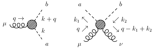
Figure 4: Vertex functions $\Gamma_{\mu ab}^{\prime\,(3)}(k,q)$ (left) and $\Gamma_{\mu\nu ab}^{\prime\,(4)}(k_{1},k_{2},q)$ (right).

It is convenient to split the full vertex functions into a bare part and a vertex correction:

$$\Gamma^{\prime\,(3)}_{\mu ab}(k,q) = g\varepsilon_{3ab}(2k+q)_{\mu}+\tilde{\Gamma}^{\prime\,(3)}_{\mu ab}(k,q)\ ,$$

$$\Gamma^{\prime\,(4)}_{\mu\nu ab}(k_{1},k_{2},q) = 2ig^{2}(\delta_{ab}-\delta_{3a}\delta_{3b})g_{\mu\nu}+\tilde{\Gamma}^{\prime\,(4)}_{\mu\nu ab}(k_{1},k_{2},q)\ .$$ (4.3)

In the vacuum the Ward-Takahshi identities are trivially satisfied. In nuclear matter, where the pion propagator is modified as discussed in the previous section, vertex corrections must be taken into account. They can be constructed by drawing all possible selfenergy insertions for the pion propagator and then couple the $\rho$ meson to all possible lines and vertices.

As a first step we will calculate the vertex corrections $\tilde{\Gamma}^{(3\,Nh)}$ and $\tilde{\Gamma}^{(4Nh)}$ which correspond to the pion selfenergy $\Sigma_{Nh}$, i.e. $Nh$ excitations without the $\pi NN$ form factor. For this purpose we have to specify the interaction of the $\rho$ meson with nucleons. To ensure gauge invariance, the interaction Lagrangians are constructed from the Lagrangians ${\cal L}_{N}$, ${\cal L}_{\pi N}$ (eqs. (3.1) and (3.2)) by minimal substitutions similar to eq. (2.2):

$${\cal L}_{\rho N} = -{g\over 2}\bar{\psi}\rho\!\!\!/\tau_{3}\psi\ ,$$ (4.4)

$${\cal L}_{\rho\pi N} = ig{f_{N}\over{m_{\pi}}}\bar{\psi}\gamma^{5}\rho\!\!\!/\vec{\tau}\psi\cdot T_{3}\vec{\phi}\ .$$ (4.5)

For the resulting vertices we again perform a non-relativistic expansion keeping only the leading order $(1/m_{N})^{0}$. The relativistic $\rho NN$ vertex and its non-relativistic expansion read

$$\Gamma_{\mu}^{(\rho NN)}=-i{g\over 2}\gamma_{\mu}\tau_{3}\longrightarrow\left\{\begin{array}[]{ll}-i{g\over 2}\tau_{3}+{\cal O}\Big{(}{1\over{m_{N}^{2}}}\Big{)}&\quad\mu=0\ ,\\ 0+{\cal O}\Big{(}{1\over{m_{N}}}\Big{)}&\quad\mu=1,2,3\ .\end{array}\right.$$ (4.6)

Thus, to order $(1/m_{N})^{0}$, the $\rho$ meson couples only to the nucleon charge and not to the convection- or magnetization currents. In fact, one could have added a term to eq. (4.4) which describes the tensor coupling of the $\rho$ meson to the anomalous magnetic moment of the nucleon and which is gauge invariant by itself. However this term would also not contribute to order $(1/m_{N})^{0}$.

The relativistic $\rho NN$ vertex fulfills the Ward-Takahashi identity

$$q^{\mu}\Gamma^{(\rho NN)}_{\mu}(p,q)=-ig{\tau_{3}\over 2}q\!\!\!/=-ig{\tau_{3}\over 2}\Big{(}S_{F}^{-1}(p+q)-S_{F}^{-1}(p)\Big{)}\ ,$$ (4.7)

where $p$ is the nucleon momentum and $q$ the momentum of the $\rho$ meson. In a consistent non-relativistic approximation an analogous relation should hold if we replace the relativistic nucleon propagator $S_{F}$ by the non-relativistic one, $G_{N}$. However, starting from the r.h.s. of eq. (4.6) the Ward-Takahashi identity is violated at order $(1/m_{N})^{1}$. To correct for this, we simply add the missing term to the $0$-component

$$\Gamma_{\mu}^{(\rho NN)}\longrightarrow\left\{\begin{array}[]{ll}-i{g\over 2}\tau_{3}{G_{N}^{-1}(p+q)-G_{N}^{-1}(p)\over{q^{0}}}+{\cal O}\Big{(}{1\over{m_{N}}}\Big{)}&\quad\mu=0\ ,\\ 0+{\cal O}\Big{(}{1\over{m_{N}}}\Big{)}&\quad\mu=1,2,3\ .\\ \end{array}\right.$$ (4.8)

At least for time-like momenta, $q$, this approximation is of the same accuracy as the non-relativistic expansion. A similar approximation is necessary for the following expression appearing in some $\rho\rho\pi\pi$ vertex corrections,

$$A_{\mu\nu} = iG_{N}(p+q_{1}-q_{2})\Gamma_{\nu}^{(\rho NN)}(p+q_{1},-q_{2})iG_{N}(p+q_{1})\Gamma_{\mu}^{(\rho NN)}(p,q_{1})iG_{N}(p)$$

$$+iG_{N}(p+q_{1}-q_{2})\Gamma_{\mu}^{(\rho NN)}(p-q_{2},q_{1})iG_{N}(p-q_{2})\Gamma_{\nu}^{(\rho NN)}(p,-q_{2})iG_{N}(p)\ .$$

Using relativistic Feynman rules, i.e. $G_{N}\rightarrow S_{F}$ and $\Gamma_{\mu}^{(\rho NN)}\rightarrow-ig{\tau_{3}\over{2}}\gamma_{\mu}$, we find

$$q_{1}^{\mu}q_{2}^{\nu}A_{\mu\nu}=-i{{g^{2}}\over{4}}\Big{(}S_{F}(p)+S_{F}(p+q_{1}-q_{2})-S_{F}(p+q_{1})-S_{F}(p-q_{2})\Big{)}\ .$$ (4.10)

Within our non-relativistic approximation, the corresponding relation (with $G_{N}$ instead of $S_{F}$ and $\Gamma_{\mu}^{(\rho NN)}$ according to eq. (4.8)) is again violated at order $(1/m_{N})^{1}$. We correct for this again by simply adding the missing term to the $00$-component:

$$A_{\mu\nu}=\left\{\begin{array}[]{ll}-i{{g^{2}}\over{4}}{1\over{q_{1}^{0}q_{2}^{0}}}\Big{(}G_{N}(p)+G_{N}(p+q_{1}-q_{2})-G_{N}(p+q_{1})-G_{N}(p-q_{2})\Big{)}&\quad\mu=\nu=0\ ,\\ 0&\quad\mbox{otherwise}\ .\\ \end{array}\right.$$ (4.11)

From ${\cal L}_{\rho\pi N}$ we deduce the $\rho\pi NN$ vertex as

$$\Gamma^{(\rho\pi NN)\,\mu}_{a}=ig{f_{N}\over{m_{\pi}}}\varepsilon_{3ba}\gamma^{5}\gamma^{\mu}\tau_{b}\longrightarrow\left\{\begin{array}[]{ll}0+{\cal O}\Big{(}{1\over{m_{N}}}\Big{)}&\quad\mu=0\ ,\\ -ig{f_{N}\over{m_{\pi}}}\varepsilon_{3ba}\sigma^{\mu}\tau_{b}+{\cal O}\Big{(}{1\over{m_{N}^{2}}}\Big{)}&\quad\mu=1,2,3\ .\end{array}\right.$$ (4.12)

We are now in place to calculate the vertex corrections corresponding to the $Nh$ selfenergy of the pion. Two of the four possible $\rho\pi\pi$ vertex correction diagrams are shown in fig. 5, the remaining ones are obtained by interchanging the pion lines. For the $\rho\rho\pi\pi$ vertex corrections, there exist sixteen possibilities to attach two $\rho$-meson lines to the $Nh$ bubble. Eight of these diagrams are shown in fig. 6 and the others can be generated by interchanging the pion lines.

Figure 5: $\rho\pi\pi$ vertex correction diagrams due to $Nh$-loops.

Figure 6: $\rho\rho\pi\pi$ vertex correction diagrams due to $Nh$-loops.

Using eqs. (4.8) and (4.12) and the definition (LABEL:DefNhLindhard), we obtain the following correction for the $\rho\pi\pi$ vertex function

$$\tilde{\Gamma}^{(3\;Nh)}_{0ab}(k,q) = -g\varepsilon_{3ab}{\vec{k}\cdot(\vec{k}+\vec{q})\over{q^{0}}}\Big{(}\Pi_{Nh}(k+q)-\Pi_{Nh}(k)\Big{)}\ ,$$

$$\tilde{\Gamma}^{(3\;Nh)}_{iab}(k,q) = g\varepsilon_{3ab}\Big{(}(k+q)_{i}\Pi_{Nh}(k+q)+k_{i}\Pi_{Nh}(k)\Big{)}\ ,$$

and the $\rho\rho\pi\pi$ vertex correction reads as

$$\tilde{\Gamma}_{00ab}^{(4\;Nh)}(k,k,q) = -ig^{2}(\delta_{ab}-\delta_{3a}\delta_{3b}){\vec{k}^{2}\over{(q^{0})^{2}}}\Big{(}\Pi_{Nh}(k+q)+\Pi_{Nh}(k-q)-2\Pi_{Nh}(k)\Big{)}\ ,$$

$$\tilde{\Gamma}_{j0ab}^{(4\;Nh)}(k,k,q) = -ig^{2}(\delta_{ab}-\delta_{3a}\delta_{3b}){k_{j}\over q^{0}}\Big{(}\Pi_{Nh}(k-q)-\Pi_{Nh}(k+q)\Big{)}\;=\;\tilde{\Gamma}_{0jab}^{(4\;Nh)}(k,k,q)\ ,$$

$$\tilde{\Gamma}_{ijab}^{(4\;Nh)}(k,k,q) = -ig^{2}(\delta_{ab}-\delta_{3a}\delta_{3b})\delta_{ij}\Big{(}\Pi_{Nh}(k-q)+\Pi_{Nh}(k+q)\Big{)}\ .$$

Since the result can be expressed through the pion selfenergy $\Pi_{Nh}$, it is quite obvious that the Ward-Takahashi identities (4.1) and (4.2) are fulfilled for a pion propagator dressed by $Nh$-loops.

The vertex corrections which correspond to the $\Delta h$ part of the pion selfenergy can be obtained in the same way. Here we start from the interaction Lagrangians

$${\cal L}_{\rho\Delta} = g\bar{\psi}_{\mu}\rho\!\!\!/T_{3}^{({3\over 2})}\psi^{\mu}-{g\over 3}\bar{\psi}_{\mu}(\gamma^{\mu}\rho_{\nu}+\gamma_{\nu}\rho^{\mu})T_{3}^{({3\over 2})}\psi^{\nu}+{g\over 3}\bar{\psi}_{\mu}\gamma^{\mu}\rho\!\!\!/T_{3}^{({3\over 2})}\gamma_{\nu}\psi^{\nu}\ ,$$ (4.15)

$${\cal L}_{\rho\pi N\Delta} = -ig{f_{\Delta}\over{m_{\pi}}}\bar{\psi}\vec{T}^{{\dagger}}\psi_{\mu}\rho^{\mu}\cdot T_{3}\vec{\phi}\quad+\quad\mbox{h.c.}\ ,$$ (4.16)

which one gets from gauging ${\cal L}_{\Delta}$ and ${\cal L}_{\pi N\Delta}$ (eqs. (3.3) and (3.4)). As stated in the previous section we include a finite width for the $\Delta$. Here one has to be careful not to violate the Ward-Takahashi identity which relates the $\rho\Delta\Delta$ vertex to the inverse $\Delta$ propagator. This is the reason why we have restricted ourselves to a constant $\Delta$ width which drops out if we take the difference between two inverse propagators.

Repeating the entire calculation for the $\Delta h$ diagrams, the result is completely analogous to eqs. (LABEL:Gamma3Nh) and (LABEL:Gamma4Nh) with the index $Nh$ replaced by $\Delta h$. For the $\rho\pi\pi$ vertex this has already been found by Chanfray and Schuck (eq. (3.7) in ref. [13]).

The next problem is to include the short-range Migdal interaction. Since the $NNNN$, $NNN\Delta$ and $NN\Delta\Delta$ vertices are momentum independent, the $\rho$ meson does not couple to these vertices. Nevertheless many additional diagrams must be calculated. An example for this class of diagrams is shown in fig. 7. It turns out that relations analogous to eqs. (LABEL:Gamma3Nh) and (LABEL:Gamma4Nh) are valid for each pion selfenergy contribution and the corresponding vertex corrections. Hence the index $Nh$ in the eqs. (LABEL:Gamma3Nh) and (LABEL:Gamma4Nh) may be omitted.

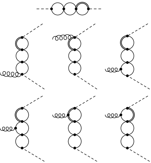
Figure 7: One contribution to the pion selfenergy and the corresponding $\rho\pi\pi$ vertex corrections.

So far the $\pi NN$ and $\pi N\Delta$ form factor $\Gamma_{\pi}$ has not been included. Naively one would expect that this form factor multiplies the $\rho\pi\pi$ vertex corrections by $\Gamma_{\pi}(\vec{k})\Gamma_{\pi}(\vec{k}+\vec{q})$ and the $\rho\rho\pi\pi$ vertex corrections by $\Gamma_{\pi}(\vec{k}_{1})\Gamma_{\pi}(\vec{k}_{2})$. However, this violates the Ward-Takahashi identities. The reason is that the $\pi NN$ ($\pi N\Delta$) form factor implies that the $\rho\pi NN$ ($\rho\pi N\Delta$) vertex must be modified. We shall do this in a systematic way as proposed in refs. [14, 26].

Formally the form factor defined in eq. (3.9) can be generated by the “propagator” $1/(-\vec{k}^{2}-\Lambda^{2})$ of a heavy particle carrying the quantum numbers of a pion (therefore called “heavy pion”), which is inserted between the physical pion propagator and the $\pi NN$ ($\pi N\Delta$) vertex (see fig. 8). Note that we have omitted the $k_{0}^{2}$ in the heavy-pion propagator, because $\Gamma_{\pi}$ depends only on the three momentum $\vec{k}$. In order to get the correct normalization of the form factor, the “vertex” where the pion is converted into the heavy pion must be assigned a factor $i\Lambda^{2}$.

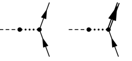
Figure 8: Insertion of the “heavy pion propagator” (dotted line) to generate the $\pi NN$ and $\pi N\Delta$ monopole form factor.

In this formalism the pion selfenergy $\Sigma^{\prime}$ corresponds to the diagram shown in the left part of fig. 9. Here $\Sigma$ again denotes the selfenergy without any form factor. Now, according to our general prescription, the $\rho\pi\pi$-vertex correction can be constructed by coupling the $\rho$ meson to this diagram in all possible ways. This leads to the three diagrams which are shown in fig. 9. The first one corresponds to the naive expectation that the vertex correction with formfactor is just the vertex correction calculated without formfactor multiplied by $\Gamma_{\pi}(\vec{k})\Gamma_{\pi}(\vec{k}+\vec{q})$. However, there are two more diagrams where the $\rho$ meson directly couples to the “heavy pion” and which are important for preserving gauge invariance.

Figure 9: Pion selfenergy (left) and $\rho\pi\pi$ vertex corrections with $\pi NN$ ($\pi N\Delta$) form factor generated by the “heavy pion”.

The vertex of the $\rho$ meson coupling to the heavy pion is almost identical to the $\rho\pi\pi$ vertex. However, since we have omitted the $k_{0}^{2}$ in the heavy pion propagator, we must also set the $\mu=0$ component of the vertex equal to zero in order to satisfy the Ward-Takahashi identity. Thus the two extra diagrams of fig. 9 contribute to the spatial components of the vertex correction only. The final result is

$$\tilde{\Gamma}^{\prime\,(3)}_{\mu ab}(k,q)=\bigg{(}\tilde{\Gamma}^{(3)}_{\mu ab}(k,q)-g\varepsilon_{3ab}(2k+q)_{i}\Big{(}{\Sigma(k+q)\over{\Lambda^{2}+(\vec{k}+\vec{q})^{2}}}+{\Sigma(k)\over{\Lambda^{2}+\vec{k}^{2}}}\Big{)}\bigg{)}\Gamma_{\pi}(\vec{k})\Gamma_{\pi}(\vec{k}+\vec{q})\ ,$$ (4.17)

where we introduced the following short-hand notation: for $\mu=0$ the term with the index $i$ should be dropped, otherwise $i=\mu$.

In the same way we can construct the $\rho\rho\pi\pi$-vertex correction with a form factor. Again starting from the pion selfenergy as shown in fig. 9 and coupling two $\rho$ mesons to this diagram we find 13 diagrams to evaluate. The result is

$$\tilde{\Gamma}^{\prime\,(4)}_{\mu\nu ab}(k,k,q) =\Bigg{\{} \tilde{\Gamma}^{(4)}_{\mu\nu ab}(k,k,q)$$

$$-ig\varepsilon_{3ca}\Big{[}{(2k-q)_{i}\over{\Lambda^{2}+(\vec{k}-\vec{q})^{2}}}\tilde{\Gamma}^{(3)}_{\nu bc}(k,-q)+{(2k+q)_{j}\over{\Lambda^{2}+(\vec{k}+\vec{q})^{2}}}\tilde{\Gamma}^{(3)}_{\mu cb}(-k-q,q)\Big{]}$$

$$-ig\varepsilon_{3bc}\Big{[}{(2k+q)_{i}\over{\Lambda^{2}+(\vec{k}+\vec{q})^{2}}}\tilde{\Gamma}^{(3)}_{\nu ac}(-k,-q)+{(2k-q)_{j}\over{\Lambda^{2}+(\vec{k}-\vec{q})^{2}}}\tilde{\Gamma}^{(3)}_{\mu ca}(k-q,q)\Big{]}$$

$$-ig^{2}(\delta_{ab}-\delta_{3a}\delta_{3b})\Big{[}{(2k-q)_{i}(2k-q)_{j}\over{\Lambda^{2}+(\vec{k}-\vec{q})^{2}}}\Big{(}{\Sigma(k-q)\over{\Lambda^{2}+(\vec{k}-\vec{q})^{2}}}+2{\Sigma(k)\over{\Lambda^{2}+\vec{k}^{2}}}\Big{)}$$

$$\hskip 91.04881pt+{(2k+q)_{i}(2k+q)_{j}\over{\Lambda^{2}+(\vec{k}+\vec{q})^{2}}}\Big{(}{\Sigma(k+q)\over{\Lambda^{2}+(\vec{k}+\vec{q})^{2}}}+2{\Sigma(k)\over{\Lambda^{2}+\vec{k}^{2}}}\Big{)}$$

$$\hskip 91.04881pt-4\delta_{ij}{\Sigma(k)\over{\Lambda^{2}+\vec{k}^{2}}}\Big{]}\quad\Bigg{\}}\Gamma_{\pi}^{2}(\vec{k})\ .$$

The meaning of the index $i$ is the same as in eq. (4.17). Similarly $j=\nu$ for $\nu=1,2,3$, whereas the corresponding terms vanish for $\nu=0$.

5 The $\rho$ Meson in Nuclear Matter

We are now ready to address the central task of our article which is the description of the $\rho$ meson in dense matter. For this we generalize the vacuum selfenergy of the $\rho$ meson as shown in fig. 1 by replacing the vacuum pion propagators and vertices by the in-medium propagators and vertex functions as calculated in the previous two sections:

$$-i\Sigma_{\mu\nu}(q) = {1\over 2}\int{d^{4}k\over{(2\pi)^{4}}}iG_{\pi}(k)\Gamma_{\mu ab}^{\prime\,(3)}(k,q)iG_{\pi}(k+q)\Gamma_{\nu ba}^{\prime\,(3)}(k+q,-q)$$ (5.1)

$$+{1\over 2}\int{d^{4}k\over{(2\pi)^{4}}}iG_{\pi}(k)\Gamma_{\mu\nu aa}^{\prime\,(4)}(k,k,q)\ .$$

The corresponding diagrams are shown in fig. 10. It is easy to see that $\Sigma_{\mu\nu}$ fulfills the transversality condition, eq. (2.5), [14]: using the Ward-Takahashi identities, eqs. (4.1) and (4.2) one gets

$$-iq^{\mu}\Sigma_{\mu\nu}(q) = {g\over 2}\varepsilon_{3ab}\int{d^{4}k\over{(2\pi)^{4}}}\Big{(}G_{\pi}(k+q)\Gamma_{\nu ba}^{\prime\,(3)}(k+q,-q)-G_{\pi}(k)\Gamma_{\nu ba}^{\prime\,(3)}(k,-q)\Big{)}\ .$$ (5.2)

Since a Pauli-Villars regularization is used we are allowed to substitute $k\longrightarrow k+q$ in the second term and the entire expression vanishes. (Obviously this would not be true if the integral was regularized by a form factor.)

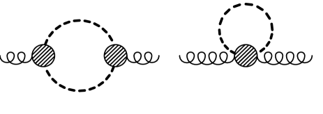
Figure 10: $\rho$-meson selfenergy in nuclear matter.

The transversality of $\Sigma_{\mu\nu}$ implies its general structure to be [27]

$$\Sigma_{\mu\nu}(q)=\Sigma_{T}(q)(P_{T})_{\mu\nu}+\Sigma_{L}(q)(P_{L})_{\mu\nu}\ ,$$ (5.3)

with the transverse and longitudinal projection operators

$$P_{T}^{\mu\nu}=\left\{\begin{array}[]{ll}0&\qquad\mu=0\quad{\rm or}\quad\nu=0\\ \delta^{\mu\nu}-\frac{q^{\mu}q^{\nu}}{\vec{q}^{\,2}}&\qquad\mu,\nu~{}{\cal 2}~{}\{1,2,3\}\end{array}\right.\quad,\qquad P_{L}^{\mu\nu}=\frac{q^{\mu}q^{\nu}}{q^{2}}-g^{\mu\nu}-P_{T}^{\mu\nu}\;.$$ (5.4)

They are both four-dimensionally transverse, but $P_{T}$ is three-dimensionally transverse, whereas $P_{L}$ is three-dimensionally longitudinal. Since in matter Lorentz invariance is not manifest because there is a preferred frame of reference in which the matter is at rest, the two functions $\Sigma_{T}$ and $\Sigma_{L}$ depend on $q^{0}$ and $|\vec{q}|$ separately.

Similarly, the in-medium $\rho$ propagator can be expressed via the projection operators $P_{T}$ and $P_{L}$ as

$$G_{\rho}^{\mu\nu}(q) = G_{\rho\,T}(q)P_{T}^{\mu\nu}+G_{\rho\,L}(q)P_{L}^{\mu\nu}+{q^{\mu}q^{\nu}\over{(m_{\rho}^{(0)})^{2}q^{2}}}$$ (5.5)

$$= {P_{T}^{\mu\nu}\over{q^{2}-(m_{\rho}^{(0)})^{2}-\Sigma_{T}(q)}}+{P_{L}^{\mu\nu}\over{q^{2}-(m_{\rho}^{(0)})^{2}-\Sigma_{L}(q)}}+{q^{\mu}q^{\nu}\over{(m_{\rho}^{(0)})^{2}q^{2}}}\ .$$

We can choose the frame of reference such that $\vec{q}$ points in the direction of the $z$-axis. In this case $\Sigma_{T}=\Sigma_{11}$ and $\Sigma_{L}=(q^{2}/q_{0}^{2})\Sigma_{33}$, i.e. it is sufficient to work with the spatial components of $\Sigma_{\mu\nu}$. Therefore we have to insert the spatial components of the vertex functions calculated in sec. 4 into eq. (5.1).

First the $k_{0}$-integration is performed. As in eq. (4.3) we split the vertex functions into a bare part and a vertex correction. The spatial components of the bare vertices do not depend on $k_{0}$. Hence, for these terms the integrands depend on $k_{0}$ through the pion propagators $G_{\pi}$ only, i.e. we have to evaluate the expressions

$$I_{1}={i\over\pi}\int dk^{0}\,G_{\pi}(k)G_{\pi}(k+q)$$ (5.6)

and

$$I_{5}={i\over\pi}\int dk^{0}\,G_{\pi}(k)\ .$$ (5.7)

The vertex corrections depend on $k_{0}$ through the pion selfenergies $\Pi^{\prime}$. This leads to additional integrals which contain pion propagators and selfenergies, for instance

$$I_{6}={i\over\pi}\int dk^{0}\,\Pi^{\prime}(k)G_{\pi}(k+q)\ ,$$ (5.8)

which arises from a vertex correction to the $\rho\rho\pi\pi$-vertex (see fig. 11). Altogether we have to evaluate seven $k_{0}$-integrals $I_{m}$, $m=1,...,7$ which are listed in appendix A.1. The spatial components of $\Sigma_{\mu\nu}$ can then be written as

$$\Sigma_{ij}(q)={g^{2}\over{2}}\;\sum_{m=1}^{7}\;\int{d^{3}k\over{(2\pi)^{3}}}\;f_{ij}^{(m)}(\vec{k},\vec{q})\;I_{m}(\vec{k},\vec{q},q_{0})$$ (5.9)

with purely real functions $f_{ij}^{(m)}(\vec{k},\vec{q})$. The explicit expressions are also given in appendix A.1.

Figure 11: Diagram representing the $I_{6}$ terms in eq. (5.9).

As mentioned earlier, the computation of $\Sigma_{ij}$ becomes quite involved if we use the exact pion selfenergies and propagators as defined in eqs. (3.5) - (3.11). Since these functions are obtained numerically, also the $k_{0}$-integrations for the functions $I_{1}$ to $I_{7}$ have to be performed numerically. Finally they have to be integrated over $|\vec{k}|$ and one angle.

Therefore we begin with the 3-level model introduced in the last paragraph of sec. 3 and will come back to the exact case later. In the 3-level model the selfenergies and propagators are given analytically (see eqs. (3.12) - (3.16)) and also allow for an analytical evaluation of the integrals $I_{1}$ to $I_{7}$. The results are listed in appendix A.2. The remaining integrations in eq. (5.9), i.e. the integration over the angle $\vartheta$ between $\vec{k}$ and $\vec{q}$ and the integration over $|\vec{k}|$, are performed numerically.

Results for the $\rho$-meson selfenergy as a function of the invariant mass $M=\sqrt{q^{2}}$ are shown in fig. 12 for different densities $\varrho$ and momenta $|\vec{q}|$. The real parts of $\Sigma_{L}$ and $\Sigma_{T}$ are displayed in the upper three panels. As discussed in ref. [14], in matter, they do no longer vanish at $M=0$ because of screening effects. The corresponding imaginary parts are shown in the lower three panels of fig. 12. Whereas in vacuum $\mbox{Im}\;\Sigma_{\mu\nu}$ vanishes below the two-pion threshold, $M=2m_{\pi}$, in matter there are new decay channels, such as $Nh$ and $\Delta h$ states, which allow for finite imaginary parts at lower invariant masses and even for $M=0$. On the other hand, the imaginary part of the $\rho$-meson selfenergy should vanish for $q^{0}\rightarrow 0$, independently of $\vec{q}$. In our model this is slightly violated because of the constant width of the $\Delta$. An energy- and momentum independent $\Delta$ width means that there is a finite probability to find a $\Delta$ with the mass of a nucleon or even below. This leads to (unphysical) decay channels of the $\rho$ meson with zero energy which are responsible for the non-vanishing selfenergy at $q^{0}=0$. However, the effect is very small. For instance, for $\varrho=2\varrho_{0}$ and $|\vec{q}|=q^{0}=0$ we find $\mbox{Im}\;\Sigma=10^{-3}{\rm GeV}^{2}$ which is not visible in fig. 12.

Figure 12: From left to right: $\Sigma=\Sigma_{T}=\Sigma_{L}$ for $|\vec{q}|=0$, $\Sigma_{T}$ and $\Sigma_{L}$ for $|\vec{q}|=0.5$ GeV at densities $\varrho=0$ (solid line), $\varrho=\varrho_{0}$ (long dashes) and $\varrho=2\varrho_{0}$ (short dashes). The calculations have been performed using the parameters of refs. [11, 12] ($\Lambda=1200$ MeV, $g^{\prime}_{11}=0.8$ and $g^{\prime}_{12}=g^{\prime}_{22}=0.5$).

In fig. 13 the longitudinal and transverse parts of the $\rho$ propagator are shown as a function of $M$ and for the same densities and momenta as the selfenergies in fig. 12. As expected, the width of the $\rho$ meson increases with density. Defining the mass of the $\rho$ meson by the zero of the real part in the propagator (“pole mass”), we find an increase with density. However, because of the strong broadening, at least at $\varrho=2\varrho_{0}$, the quasiparticle concept breaks down. At this density one can also see that the spectral function, i.e. the imaginary part of the propagator, develops two maxima, one above and one below the vacuum $\rho$-meson peak. For $\vec{q}=0$ this was already found in refs. [13, 14]. At finite $\vec{q}$, however, the transverse and the longitudinal propagator behave rather differently.

Figure 13: From left to right: $G_{\rho}=G_{\rho\,T}=G_{\rho\,L}$ for $|\vec{q}|=0$, $G_{\rho\,T}$ and $G_{\rho\,L}$ for $|\vec{q}|=0.5$ GeV at densities $\varrho=0$ (solid line), $\varrho=\varrho_{0}$ (long dashes) and $\varrho=2\varrho_{0}$ (short dashes). The calculations have been performed using the parameters of refs. [11, 12] ($\Lambda=1200$ MeV, $g^{\prime}_{11}=0.8$ and $g^{\prime}_{12}=g^{\prime}_{22}=0.5$).

This can be seen even better in fig. 14 where the imaginary parts of $G_{\rho\,T}$ and $G_{\rho\,L}$ at $\varrho=2\varrho_{0}$ are plotted as functions of $|\vec{q}|$ and $M$. The two branches we have seen in fig. 13 are clearly visible in both functions. Note that the lower branch of $\mbox{Im}\,G_{\rho\,T}$ comes down to lower invariant masses with increasing $|\vec{q}|$ and finally reaches $M=0$. This will become important later on.

Figure 14: Imaginary part of the transverse and longitudinal $\rho$ propagator $G_{\rho\,T}$ and $G_{\rho\,L}$ at $\varrho=2\varrho_{0}$ as a function of the invariant mass $M$ and the momentum $|\vec{q}|$. The calculations have been performed using the parameters of refs. [11, 12] ($\Lambda=1200$ MeV, $g^{\prime}_{11}=0.8$ and $g^{\prime}_{12}=g^{\prime}_{22}=0.5$).

For the interpretation we take the imaginary part of the propagator:

$$\mbox{Im}\;G_{\rho\,T,L}(q)={\mbox{Im}\;\Sigma_{T,L}(q)\over{(q^{2}-(m_{\rho}^{(0)})^{2}-\mbox{Re}\,\Sigma_{T,L}(q))^{2}}+(\mbox{Im}\,\Sigma_{T,L}(q))^{2}}\ .$$ (5.10)

Approximately, the maxima of $\mbox{Im}\;G_{\rho\,T,L}$ correspond to maxima of $\mbox{Im}\;\Sigma_{T,L}$ or to minima of the denominator of eq. (5.10). In vacuum only the latter are present. With increasing density the vacuum peaks are pushed to higher $q^{2}$ as a consequence of an increased real part of the selfenergy. This explains the branches of $\mbox{Im}\;G_{\rho\,T}$ and $\mbox{Im}\;G_{\rho\,L}$ at higher $M$. The lower branches correspond to $\mbox{Im}\;\Sigma_{T,L}$ and thus, according to eq. (5.9), to the imaginary parts of the functions $I_{1}$ to $I_{7}$.

From the explicit expressions given in appendix A.2 (eqs. (A.12) - (A.18)) and neglecting the finite $\Delta$ width for the moment we find:

$$\mbox{Im}\,I_{m}(\vec{k},\vec{q},q_{0})\;=\;\sum_{i,j=1}^{3}\varphi_{ij}^{(m)}(\vec{k},\vec{q})\;\delta(q_{0}^{2}-(\omega_{i}(\vec{k})+\omega_{j}(\vec{k}+\vec{q}))^{2})\qquad\rm{for\quad m=1,...,4}\;,$$ (5.11)

$$\mbox{Im}\,I_{6}(\vec{k},\vec{q},q_{0})\;=\;\sum_{i=1}^{2}\sum_{j=1}^{3}\varphi_{ij}^{(6)}(\vec{k},\vec{q})\;\delta(q_{0}^{2}-(\Omega_{i}(\vec{k})+\omega_{j}(\vec{k}+\vec{q}))^{2})$$ (5.12)

and

$$\mbox{Im}\,I_{5}(\vec{k},\vec{q},q_{0})\;=\;\mbox{Im}\,I_{7}(\vec{k},\vec{q},q_{0})\;=\;0\;,$$ (5.13)

where $\varphi_{ij}^{(m)}(\vec{k},\vec{q})$ are some real, well-behaved functions. Including the $\Delta$ width basically leads to some “smoothing” of the $\delta$-functions.

The structure of the expressions for $\mbox{Im}\,I_{1}$ to $\mbox{Im}\,I_{4}$ suggests the following physical interpretation: in matter the decay of the $\rho$ meson into two pions is replaced by the decay into two longitudinal quasiparticles with dispersion relations $\omega_{i}$ and $\omega_{j}$ (see eq. (3.16)), i.e. $(Nh)_{L}$, $\pi$ or $(\Delta h)_{L}$ quasiparticles. The situation is slightly different for $I_{6}$ which originates from a vertex correction to the $\rho\rho\pi\pi$-four point vertex (see fig. 11). To this diagram also transverse $Nh$ and $\Delta h$ excitations contribute which have the dispersion relations $\Omega_{1}$ and $\Omega_{2}$. In fact, as explained in appendix A.1, the decay into two longitudinal modes can be separated out and $\mbox{Im}\,I_{6}$ describes the decay of the $\rho$ meson into one longitudinal quasiparticle and one transverse $Nh$ or $\Delta h$ excitation.

Due to their small strength, $S_{1}$, the decay channels involving one or two $(Nh)_{L}$ quasiparticles are relatively unimportant. The decay into two pion quasiparticles is suppressed by vertex corrections, as already shown in refs. [13, 28]. Therefore the most important contributions to $\mbox{Im}\,I_{1}$ to $\mbox{Im}\,I_{4}$ come from the decay $\rho\rightarrow\pi(\Delta h)_{L}$. Similarly $\mbox{Im}\,I_{6}$ is dominated by the decay $\rho\rightarrow\pi(\Delta h)_{T}$.

In order to identify these two modes in the spectral function we realize that the pionic branch has most of its strength at low momenta (see fig. 3). Therefore a $\rho$ meson with momentum $\vec{q}$ should predominantly decay into a pion with momentum $\vec{k}\approx 0$ and a $\Delta h$ pair with momentum close to $\vec{q}$. The corresponding invariant masses

$$M_{\rho\rightarrow\pi(\Delta h)_{L}} \approx \sqrt{\Big{(}m_{\pi}+\omega_{3}(\vec{q})\Big{)}^{2}-\vec{q}^{\,2}}\ ,$$

$$M_{\rho\rightarrow\pi(\Delta h)_{T}} \approx \sqrt{\Big{(}m_{\pi}+\Omega_{2}(\vec{q})\Big{)}^{2}-\vec{q}^{\,2}}\ ,$$ (5.14)

are shown in fig. 15 for $\varrho=2\varrho_{0}$. They are in good qualitative agreement with the structures seen in the imaginary part of the $\rho$ propagator: We can identify the lower branch of $\mbox{Im}\,G_{\rho\,L}$ with the decay mode $\rho\rightarrow\pi(\Delta h)_{L}$ and the lower branch of $\mbox{Im}\,G_{\rho\,T}$ with the decay mode $\rho\rightarrow\pi(\Delta h)_{T}$. Therefore this structure of $\mbox{Im}\,G_{\rho\,T}$ is mainly a consequence of the vertex correction in fig. 11.

Figure 15: Invariant mass M of the $\rho$ meson decaying into a transverse (solid line) or longitudinal (dashed line) $\Delta h$ pair, resulting from the approximate formulae eq. (5.14).

All results presented so far have been calculated within the 3-level model, i.e. the Fermi motion of the nucleons has been neglected. In the final part of this section we want to test the quality of this approximation. Using spectral representations for the pion propagator $G_{\pi}$ and the selfenergy $\Pi^{\prime}$,

$$G_{\pi}(k_{0},\vec{k}) = -{1\over\pi}\int_{0}^{\infty}d\omega^{2}{\mbox{Im}\,G_{\pi}(\omega,\vec{k})\over{k_{0}^{2}-\omega^{2}+i\varepsilon}}\ ,$$ (5.15)

$$\Pi^{\prime}(k_{0},\vec{k}) = -{1\over\pi}\int_{0}^{\infty}d\omega^{2}{\mbox{Im}\,\Pi^{\prime}(\omega,\vec{k})\over{k_{0}^{2}-\omega^{2}+i\varepsilon}}\ ,$$ (5.16)

the imaginary parts of the integrals $I_{1}$ to $I_{4}$ and $I_{6}$ reduce to integrals from $0$ to $q^{0}$, e.g.

$$\mbox{Im}\,I_{6}(\vec{k},\vec{q},q_{0})=-{2\over\pi}\int_{0}^{q_{0}}d\omega\;\mbox{Im}\,\Pi^{\prime}(\omega,\vec{k})\mbox{Im}\,G_{\pi}(q_{0}-\omega,\vec{k}+\vec{q})\ ,$$ (5.17)

and similar expressions for $\mbox{Im}\,I_{1}$ to $\mbox{Im}\,I_{4}$, while $\mbox{Im}\,I_{5}$ and $\mbox{Im}\,I_{7}$ vanish. From the structure of these integrals one sees immediately that the imaginary part of the $\rho$-meson selfenergy vanishes for $q_{0}\rightarrow 0$, as it should. As discussed above, because of the constant $\Delta$ width this was not exactly true for the results shown before. However, the dispersion relations, eqs. (5.15) and (5.16), are also slightly violated by the constant $\Delta$ width and the two effects cancel to some extend giving the expressions like eq. (5.17) the correct behavior for $q_{0}\rightarrow 0$.

The expressions for $\mbox{Im}\,I_{m}$ and the remaining angular and momentum integration in eq. (5.9) can be evaluated numerically. Some results for the imaginary part of the $\rho$-meson selfenergy at $\varrho=2\varrho_{0}$ are shown in fig. 16. Obviously the difference to the results obtained within the three level model is small. This is somewhat surprising since the 3-level model is known to be a quite poor approximation to the pion selfenergy, at least in the domain of the $Nh$-excitations. However, after integrating over momenta, details of the pion spectral function are “washed out” and only gross features are important which are correctly reproduced by the 3-level model. Of course the approximation becomes even better at lower densities where the effect of Fermi motion is less important.

Figure 16: From left to right: Imaginary part of $\Sigma=\Sigma_{T}=\Sigma_{L}$ for $|\vec{q}|=0$, $\Sigma_{T}$ and $\Sigma_{L}$ for $|\vec{q}|=0.5$ GeV, at density $\varrho=2\varrho_{0}$. Solid line: full calculation, dashes: 3-level model.

6 Applications: Photoabsorption and Dilepton Production

In this section we apply our model to the calculation of electromagnetic processes, focusing on the effect of the 3-momentum dependence of the pionic part of the $\rho$-meson selfenergy.

We begin with the calculation of the total absorption cross section of real photons on nucleons and nuclei [24]. In nuclear matter the inclusive cross section per nucleon for a photon with momentum $\vec{q}$ and polarization vector $\epsilon_{\mu}(\vec{q},\lambda)$ is given by

$${\sigma\over A}={1\over{\varrho}}\,{e^{2}\over{2|\vec{q}|}}\sum_{f}\Big{|}\epsilon_{\mu}(\vec{q},\lambda)\langle{f}|J^{\mu}(0)|{\Phi_{0}}\rangle\Big{|}^{2}(2\pi)^{4}\delta(p_{f}-q)\ .$$ (6.1)

In this expression $|{f}\rangle$ is the unobserved final hadronic state, $|{\Phi_{0}}\rangle$ specifies the ground state of nuclear matter, and $J^{\mu}$ denotes the electromagnetic current operator.

This expression can be related to the current-current correlation function

$$J^{\mu\nu}(q)=-i\int d^{4}x\,e^{iq\cdot x}\langle{\Phi_{0}}|T\Big{(}J^{\mu}(x)J^{\nu}(0)\Big{)}|{\Phi_{0}}\rangle\ .$$ (6.2)

Inserting a complete set of energy and momentum eigenstates between the two current operators and taking the imaginary part, we find

$${\sigma\over A}=-{1\over{\varrho}}\,{e^{2}\over{|\vec{q}|}}\,\epsilon_{\mu}(\vec{q},\lambda)\epsilon_{\nu}(\vec{q},\lambda)\,\mbox{Im}\,J^{\mu\nu}(q)\ .$$ (6.3)

In the VDM $J^{\mu}$ is a linear combination of the $\rho$, $\omega$ and $\phi$ field operators. Neglecting the isoscalar contributions, the current field identity reads

$$J^{\mu}(x)={(m_{\rho}^{(0)})^{2}\over g}\rho^{\mu}(x)\ ,$$ (6.4)

i.e. $J^{\mu\nu}(q)$ is proportional to the $\rho$ propagator $G_{\rho}^{\mu\nu}(q)$. Because of the transverse polarization of the photon only $G_{\rho\,T}^{\mu\nu}(q)$ contributes, and we finally obtain

$${\sigma\over A}=-{1\over{\varrho}}\,{e^{2}\over{|\vec{q}|}}\,{(m_{\rho}^{(0)})^{4}\over{g^{2}}}\,{\mbox{Im}\,\Sigma_{T}(q)\over{|(m_{\rho}^{(0)})^{2}+\Sigma_{T}(q)|^{2}}}\ .$$ (6.5)

It is obvious that the 3-momentum dependence of the $\rho$-meson selfenergy is necessary for the calculation of photoabsorption cross sections within the VDM: Since $M=0$ for real photons, $|\vec{q}|$ is the only variable the cross section can depend on.

For very small densities, $\varrho$, eq. (6.5) describes the photoabsorption cross section of a single nucleon. Since the $\rho$-meson selfenergy in vacuum vanishes for $q^{2}=0$, the limit $\varrho\rightarrow 0$ is well defined and can be written as

$$\lim_{\varrho\rightarrow 0}{\sigma\over A}=-{e^{2}\over{|\vec{q}|}}\,{1\over{g^{2}}}\,\lim_{\varrho\rightarrow 0}{\mbox{Im}\Sigma_{T}(q)\over{\varrho}}\ .$$ (6.6)

In this limit, interferences between different contributions to $\Sigma_{T}$ vanish and only contributions to $\Sigma_{T}$ linear in $\varrho$ survive, i.e. diagrams containing exactly one $Nh$ or $\Delta h$ loop. Of course, describing photoabsorption on a single nucleon, the creation of a hole is more conveniently interpreted as the destruction of the initial nucleon.

Since the cross section is proportional to the imaginary part of $\Sigma_{T}$, the processes which contribute correspond to cuts through the transverse part of the $\rho$-meson selfenergy. Our model, as described in the previous section, leads to the non-resonant background of the photoabsorption cross section, e.g. $\gamma\rightarrow\pi+Nh$ or $\gamma\rightarrow\pi+\Delta h$. The threshold for such processes on a single nucleon at rest is $|\vec{q}|>150$ MeV.

Our results for the non-resonant background of the photoabsorption cross section of the nucleon are shown in the left panel of fig. 17. For comparison we also display the experimental data, averaged over protons [29] and neutrons [30]. The short-dashed line corresponds to a form factor cutoff $\Lambda=1200$ MeV as used in the Bonn potential [25, 34] and in refs. [11, 12]. In this case, the background alone exceeds the data for $q_{0}>800$ MeV, revealing the cutoff as too large for the present purposes. The solid line was obtained with $\Lambda=550$ MeV, which does not contradict the data.

Our results are in line with the well-known fact that for many applications a much softer form factor is needed than the one used in the Bonn potential (e.g. $\pi N$ scattering in the Chew-Low model [35]: $\Lambda_{\pi NN}\approx 520$ MeV, $\pi^{0}$ photoproduction [36]: $\Lambda_{\pi N\Delta}=300$ MeV, deep inelastic lepton scattering [37]: $\Lambda_{\pi NN(\Delta)}<500$ MeV). In the cloudy bag model for the nucleon [38] the form factor has the form $3j_{1}(|\vec{k}|R)/(|\vec{k}|R)$, which for $R=0.8$ fm corresponds to a monopole with $\Lambda_{\pi NN(\Delta)}=\sqrt{10}/R\approx 780$ MeV [25]. This value is similar to a result from lattice QCD [39], $\Lambda_{\pi NN}=(750\pm 140)$ MeV.

Figure 17: Left panel: Photoabsorption cross section of the nucleon. The data are the averages of the total cross sections for protons [29] and neutrons [30]. The theoretical calculations correspond to the non-resonant background only. They were obtained from eq. (6.5) with $\varrho=0.052\,\varrho_{0}$ and cutoff parameters $\Lambda=1200$ MeV (short-dashed line) and $\Lambda=550$ MeV (all other lines). The background represented by the solid line is also separated into the processes $\gamma N\rightarrow\pi N$ (long-dashed line) and $\gamma N\rightarrow\pi\Delta$ (dashed-dotted line). Right panel: Photoabsorption cross section per nucleon of uranium. The data are averages of the data from refs. [31, 32, 33], the background has been calculated using eq. (6.5) with $\varrho=0.8\,\varrho_{0}$, $\Lambda=550$ MeV, $g^{\prime}_{11}=0.6$ and $g^{\prime}_{12}=g^{\prime}_{22}=0.25$. The dashed line was obtained within the 3-level model. The solid line corresponds to an improved calculation with the imaginary part of the $\rho$-meson selfenergy calculated with Fermi motion while for the real part the result of the 3-level model was taken.

In fig. 17 we also show a decomposition of the background into the processes $\gamma N\rightarrow\pi N$ (long-dashed line) and $\gamma N\rightarrow\pi\Delta$ (dashed-dotted line). Since the $\Delta$ resonance decays into $\pi N$ (implicitly contained in our model through the constant width of the $\Delta$) the dashed-dotted line can be identified with the two-pion background while the long-dashed line corresponds to the single-pion background. The latter is somewhat larger than the single-pion background found by Effenberger et al. [40] in an analysis of the $\gamma N\rightarrow\pi N$ data. This might indicate that our formfactor should be reduced even further .

For a realistic description of the photoabsorption resonance-hole excitations, like $\gamma\rightarrow\Delta h$ or $\gamma\rightarrow N^{*}(1520)h$, have to be taken into account in addition to the non-resonant background. The resonant contributions to the $\rho$-meson selfenergy have already been worked out in a momentum dependent way in ref. [12] and can therefore easily be added to our model. This has been done in ref. [24] and we refer to this publication for more details.

In the right panel of fig. 17 we show our results for the photoabsorption on nuclei together with the experimental data for uranium [31, 32, 33]. The calculations have been done using $\Lambda=550$ MeV, $g^{\prime}_{11}=0.6$ and $g^{\prime}_{12}=g^{\prime}_{22}=0.25$. As an average density in finite nuclei we took $\varrho=0.8\varrho_{0}$. The dashed line was obtained within the 3-level model. The solid line corresponds to an improved calculation with the imaginary part of the $\rho$-meson selfenergy calculated as outlined in the end of section 5, i.e. including Fermi motion. For the real part we kept the result of the 3-level model. Obviously for energies greater than $\sim 150$ MeV the differences between the two approximations are small. At lower energies the differences in the selfenergy, although still small in absolute units, are enhanced by the factor $1/|\vec{q}|$ in eq. (6.5). Therefore the 3-level model should not be trusted in this regime.

In contrast to the photoabsorption on a single nucleon, in nuclear matter there is no threshold at $|\vec{q}|\simeq 150$ MeV. For instance, processes mediated by meson-exchange currents, like $\gamma\rightarrow\pi\pi\rightarrow(Nh)(Nh)$ allow for the absorption of photons with much lower energies. Of course our model cannot describe the giant resonances at very low energies, but the pionic background contributes considerably to the “dip region” at $|\vec{q}|\sim 150$ MeV.

Again, for a realistic description of the data resonant diagrams have to be taken into account. More details about this can be found in ref. [24].

Finally we turn to the calculation of dilepton rates in hot nuclear matter. In the VDM the rate of $e^{+}e^{-}$ pairs with total 4-momentum $q$ produced per volume $d^{3}x$ is given by [13]:

$${dN_{e^{+}e^{-}}\over{d^{4}xd^{4}q}}={\alpha^{2}\over{3\pi^{3}M^{2}}}\,{1\over{e^{q^{0}/T}-1}}\,{(m_{\rho}^{(0)})^{4}\over{g^{2}}}\,g^{\mu\nu}\,\mbox{Im}\,G_{\rho\,\mu\nu}^{R}(q;\,T)\ .$$ (6.7)

Here $\alpha=e^{2}/(4\pi)$ is the fine structure constant, $M=\sqrt{q^{2}}$ the invariant mass of the dilepton pair, and $T$ the temperature of the hadronic matter. $G_{\rho}^{R}(q;\,T)$ is the retarded $\rho$ propagator at temperature $T$ and baryon density $\varrho$. Thus eq. (6.7) depends on temperature through the Bose factor $1/(e^{q^{0}/T}-1)$ and through the retarded propagator. Since in sec. 5 the $\rho$ propagator was calculated for $T=0$ only we approximate

$$\mbox{Im}\,G_{\rho}^{R}(q;\,T)\approx\mbox{Im}\,G_{\rho}(q;\,T=0)\ ,$$ (6.8)

but keep the temperature dependence through the Bose factor. (Note that at $T=0$ the imaginary parts of the retarded propagator $G_{\rho}^{R}$ and the time-ordered one $G_{\rho}$ are equal.)

In fig. 18 the dilepton rates for $T=150$ MeV and $\varrho=\varrho_{0}$ are shown. In the calculations we used the parameters obtained from the fit to the photoabsorption spectra [24], i.e. $\Lambda=550$ MeV, $g^{\prime}_{11}=0.6$ and $g^{\prime}_{12}=g^{\prime}_{22}=0.25$. The solid line corresponds to our model as described above. For $M\sim 0.2$ - $0.6$ GeV it is in fair agreement with the ‘pion + one loop’ result of Steele et al. [44]. However, whereas these authors find almost no medium effect at and above the free $\rho$-meson mass, in our calculation the vacuum peak is strongly reduced and we find enhanced rates at higher invariant masses. (For comparison see the dotted line which has been calculated using the $\rho$ propagator in vacuum.)

Figure 18: Dilepton rates for $\varrho=\varrho_{0}$ and $T=150$ MeV calculated from eq. (6.7) with different approximations to the retarded $\rho$ propagator $G_{\rho}^{R}(q^{0},\vec{q};\,T)$: $G_{\rho}(q^{0},\vec{q};\,T=0)$ (solid line), $G_{\rho}(M,\vec{q}=0;\,T=0)$ (dashed line), and $G_{\rho}^{\mathit{vac}}(q^{0},\vec{q};\,T=0)$ (dotted line). The parameters are $\Lambda=550$ MeV, $g^{\prime}_{11}=0.6$ and $g^{\prime}_{12}=g^{\prime}_{22}=0.25$.

We also show the result of a calculation neglecting the $\vec{q}$ dependence, i.e. using the approximation of refs. [11, 12], $\mbox{Im}\,G_{\rho}(q^{0},\vec{q})\approx\mbox{Im}\,G_{\rho}(M,\vec{q}=0)$ (dashed line). Whereas the momentum dependence does not change very much for larger invariant masses, for $M$ below $\sim 300$ MeV the results including the $\vec{q}$ dependence of $G_{\rho}$ (solid line) are significantly enhanced as compared to the calculation without $\vec{q}$ dependence (dashed line). This can be explained as follows: As discussed in sec. 5, the $\rho$ meson strongly mixes with $\pi(\Delta h)_{T}$ states and the invariant mass of these states decreases with increasing $\vec{q}$ and finally reaches zero (see figs. 14 and 15). Because of the factor $1/M^{2}$ in eq. (6.7) this leads to a strong enhancement of the dilepton rate at small $M$. (Of course, the divergence at $M=0$ is only an artifact of neglecting the electron mass in the derivation of eq. (6.7).)

Again, in a realistic calculation resonance contributions of the type $\rho\rightarrow Bh$ have to be taken into account [12, 15].

7 Summary and Conclusions

We have extended hadronic models for $\rho$-meson propagation in cold nuclear matter involving medium modifications of the pion propagator to include finite 3-momenta. The starting point was the $\rho$ propagator in vacuum with a bare propagator dressed by $\pi\pi$-loops. In matter, the pions are renormalized through particle-hole and $\Delta$-hole excitations correlated by Migdal parameters. We use a 3-momentum dependent monopole form factor to cut off higher momenta at the $\pi NN$- and $\pi N\Delta$-vertices. For numerical convenience, in most of our calculations the dressed pion propagator was approximated by the so-called “3-level model” which is obtained from the exact propagator by neglecting the Fermi motion of the nucleons. This approximation was found to be excellent for our purposes (see figs. 16 and 17).

Because of the medium modifications of its pion cloud, the properties of the $\rho$-meson become modified as well in matter. Guided by Ward-Takahashi identities, we have calculated vertex corrections to the $\rho\pi\pi$- and $\rho\rho\pi\pi$-vertices in order to preserve gauge invariance. For the resulting in-medium $\rho$ propagator these vertex corrections turned out to be particularly important to shift part of the strength down to the regime of low invariant masses. The main effect could be attributed to the decay of the $\rho$ into a pion and a spin-transverse $\Delta$-hole excitation. For $|\vec{q}|=0$ this branch was already found by Chanfray and Schuck [13] and by Herrmann et al. [14]. However, with increasing $|\vec{q}|$ it comes down to even lower invariant masses and eventually crosses the $M=0$ line.

As one application of the model we calculated the non-resonant background for photoabsorption on nucleons and nuclei. In order to be consistent with the experimental data, the cutoff parameter which enters the $\pi NN$- and $\pi N\Delta$-form factor had to be reduced from $1200$ MeV as used in earlier calculations [11, 12] to $550$ MeV. This example shows the importance of constraining the model parameters from experimental data. As discussed in section 6, there are indications from other observables, like more exclusive photoabsorption data (see ref. [40]) or pion-induced $\rho$-meson production [41] that a further reduction of the cutoff might be necessary. This is presently under investigation.

Finally we have studied the consequences of the 3-momentum dependence of the $\rho$-meson propagator for dilepton production rates in hot and dense matter. Compared to a calculation where the $|\vec{q}|$-dependence was neglected we found almost no difference for invariant masses above $\sim 400$ MeV but a strong enhancement of the rates at lower $M$. This is related to the $\pi(\Delta h)_{T}$-branch as discussed above.

In the present article we have concentrated on the pion-loop contribution to the $\rho$-meson selfenergy. However, realistic calculations require to account for contributions arising from direct resonance formation $\rho\rightarrow Bh$ [12, 15, 16]. In fact, the medium modifications of the $\rho$ propagator associated with the pionic part of the selfenergy are substantially decreased by the use of much softer $\pi NN$ and $\pi N\Delta$ form factors. This increases the relative importance of the resonances as compared to earlier versions of the model where a larger cutoff was used [12]. As long as interferences induced by explicit resonance decays are neglected, the resonance-hole diagrams can be evaluated separately and simply added to the pionic selfenergy contributions [24]. Ultimately, one should take into account the resonance decays into $\pi N$ and $\rho N$ in a selfconsistent fashion [16], which also implies a better description of the $\Delta$ width.

ACKNOWLEDGMENTS

We are grateful for productive conversations with G. Chanfray. One of us (RR) acknowledges support from the A.-v.-Humboldt-foundation as a Feodor-Lynen fellow and from the U.S. Department of Energy under Grant No. DE-FG02-88ER40388.

Appendix A $\rho$ Meson Selfenergy at Finite Density

A.1 General Expressions for the Spatial Components

As described in sec. 5, the spatial components of the $\rho$-meson selfenergy are calculated by inserting the spatial components of the vertex functions calculated in sec. 4 into eq. (5.1). If we split the vertex functions into bare vertices and vertex corrections, as in eq. (4.3), the selfenergy becomes a sum of seven terms:

$$\Sigma_{ij}(q) = {g^{2}\over{4}}\int{d^{3}k\over{(2\pi)^{3}}}\bigg{(}(2k+q)_{i}(2k+q)_{j}\,I_{1}$$ (A.1)

$$+4{(k_{i}(\Lambda^{2}-\vec{k}^{2})-q_{i}\vec{k}^{2})(2k+q)_{j}\over{\Lambda^{2}+(\vec{k}+\vec{q})^{2}}}\,I_{2}$$

$$+2{(k_{i}(\Lambda^{2}-\vec{k}^{2})-q_{i}\vec{k}^{2})(k_{j}(\Lambda^{2}-\vec{k}^{2})-q_{j}\vec{k}^{2})\over{(\Lambda^{2}+(\vec{k}+\vec{q})^{2})^{2}}}\,\tilde{I}_{3}$$

$$+2{(k_{i}(\Lambda^{2}-\vec{k}^{2})-q_{i}\vec{k}^{2})(k_{j}(\Lambda^{2}-(\vec{k}+\vec{q})^{2})+q_{j}\Lambda^{2})\over{(\Lambda^{2}+(\vec{k}+\vec{q})^{2})(\Lambda^{2}+\vec{k}^{2})}}\,I_{4}$$

$$+2\,I_{5}$$

$$+2{(\Lambda^{2}+\vec{k}^{2})\delta_{ij}-(2k+q)_{i}(2k_{j}\Lambda^{2}-q_{j}\vec{k}^{2})\over{(\Lambda^{2}+(\vec{k}+\vec{q})^{2})^{2}}}\,I_{6}$$

$$-4\Big{(}{\vec{k}^{2}\delta_{ij}\over{\Lambda^{2}+\vec{k}^{2}}}+{(2k+q)_{i}(k_{j}(\Lambda^{2}-\vec{k}^{2})-q_{j}\vec{k}^{2})\over{(\Lambda^{2}+(\vec{k}+\vec{q})^{2})(\Lambda^{2}+\vec{k}^{2})}}\Big{)}\,I_{7}\bigg{)}$$

$$+(i\longleftrightarrow j)\ .$$

with

$$I_{1} = {i\over\pi}\int dk^{0}\,G_{\pi}(k)G_{\pi}(k+q)\ ,$$ (A.2)

$$I_{2} = {i\over\pi}\int dk^{0}\,\Pi^{\prime}(k)G_{\pi}(k)G_{\pi}(k+q)\ ,$$ (A.3)

$$\tilde{I}_{3} = {i\over\pi}\int dk^{0}\,\Pi^{\prime\,2}(k)G_{\pi}(k)G_{\pi}(k+q)\ ,$$ (A.4)

$$I_{4} = {i\over\pi}\int dk^{0}\,\Pi^{\prime}(k)G_{\pi}(k)\Pi^{\prime}(k+q)G_{\pi}(k+q)\ ,$$ (A.5)

$$I_{5} = {i\over\pi}\int dk^{0}\,G_{\pi}(k)\ ,$$ (A.6)

$$I_{6} = {i\over\pi}\int dk^{0}\,\Pi^{\prime}(k)G_{\pi}(k+q)\ ,$$ (A.7)

$$I_{7} = {i\over\pi}\int dk^{0}\,\Pi^{\prime}(k)G_{\pi}(k)\ .$$ (A.8)

It is useful to rearrange these terms slightly [13]: in the integrals $I_{2}$, $\tilde{I}_{3}$, $I_{4}$ and $I_{7}$ the vertex corrections $\Pi^{\prime}$ are always coupled to a pion propagator of the same momentum. Therefore, only the spin-longitudinal $Nh$ or $\Delta h$ excitations contained in $\Pi^{\prime}$ can contribute to these integrals. This is different for $I_{6}$. Here longitudinal and transverse $Nh$ and $\Delta h$ excitations of the vertex correction can contribute, because they are not coupled to a pion. However, we can separate longitudinal and transverse $Nh$ and $\Delta h$ excitations in the $I_{6}$ term, and combine the longitudinal part with the $\tilde{I}_{3}$ term. To that end, we define the longitudinal spin-isospin response function,

$$\Pi_{L}^{\prime}(k)=\Pi^{\prime}(k)+\Pi^{\prime}(k)\vec{k}^{2}G_{\pi}(k)\Pi^{\prime}(k)=(k^{2}-m_{\pi}^{2})\Pi^{\prime}(k)G_{\pi}(k)\ ,$$ (A.9)

and an integral similar to $I_{6}$,

$$I_{3}={i\over\pi}\int dk^{0}\,\Pi^{\prime}_{L}(k)G_{\pi}(k+q)=\vec{k}^{2}\tilde{I}_{3}+I_{6}\ .$$ (A.10)

With this abbreviation we can write

$$\Sigma_{ij}(q) = {g^{2}\over{4}}\int{d^{3}k\over{(2\pi)^{3}}}\bigg{(}(2k+q)_{i}(2k+q)_{j}\,I_{1}$$ (A.11)

$$+4{(k_{i}(\Lambda^{2}-\vec{k}^{2})-q_{i}\vec{k}^{2})(2k+q)_{j}\over{\Lambda^{2}+(\vec{k}+\vec{q})^{2}}}\,I_{2}$$

$$+2{(k_{i}(\Lambda^{2}-\vec{k}^{2})-q_{i}\vec{k}^{2})(k_{j}(\Lambda^{2}-\vec{k}^{2})-q_{j}\vec{k}^{2})\over{\vec{k}^{2}(\Lambda^{2}+(\vec{k}+\vec{q})^{2})^{2}}}\,I_{3}$$

$$+2{(k_{i}(\Lambda^{2}-\vec{k}^{2})-q_{i}\vec{k}^{2})(k_{j}(\Lambda^{2}-(\vec{k}+\vec{q})^{2})+q_{j}\Lambda^{2})\over{(\Lambda^{2}+(\vec{k}+\vec{q})^{2})(\Lambda^{2}+\vec{k}^{2})}}\,I_{4}$$

$$+2\,I_{5}$$

$$+2{(\Lambda^{2}+\vec{k}^{2})^{2}\over{(\Lambda^{2}+(\vec{k}+\vec{q})^{2})^{2}}}\Big{(}\delta_{ij}-{k_{i}k_{j}\over{\vec{k}^{2}}}\Big{)}\,I_{6}$$

$$-4\Big{(}{\vec{k}^{2}\delta_{ij}\over{\Lambda^{2}+\vec{k}^{2}}}+{(2k+q)_{i}(k_{j}(\Lambda^{2}-\vec{k}^{2})-q_{j}\vec{k}^{2})\over{(\Lambda^{2}+(\vec{k}+\vec{q})^{2})(\Lambda^{2}+\vec{k}^{2})}}\Big{)}\,I_{7}\bigg{)}$$

$$+(i\longleftrightarrow j)\ .$$

A.2 3-Level Model

Within the 3-level model the integrals $I_{1}$ to $I_{7}$ can be evaluated analytically:

$$I_{1} = \sum_{i=1}^{3}\sum_{j=1}^{3}{S_{i}(\vec{k})\over{\omega_{i}(\vec{k})}}\,{S_{j}(\vec{k}+\vec{q})\over{\omega_{j}(\vec{k}+\vec{q})}}\,{\omega_{i}(\vec{k})+\omega_{j}(\vec{k}+\vec{q})\over{q_{0}^{2}-(\omega_{i}(\vec{k})+\omega_{j}(\vec{k}+\vec{q}))^{2}}}\ ,$$ (A.12)

$$I_{2} = \sum_{i=1}^{3}\sum_{j=1}^{3}{C_{i}(\vec{k})\over{\omega_{i}(\vec{k})}}\,{S_{j}(\vec{k}+\vec{q})\over{\omega_{j}(\vec{k}+\vec{q})}}\,{\omega_{i}(\vec{k})+\omega_{j}(\vec{k}+\vec{q})\over{q_{0}^{2}-(\omega_{i}(\vec{k})+\omega_{j}(\vec{k}+\vec{q}))^{2}}}\ ,$$ (A.13)

$$I_{3} = \sum_{i=1}^{3}\sum_{j=1}^{3}{(\omega_{i}^{2}(\vec{k})-\omega_{\pi}^{2}(\vec{k}))C_{i}(\vec{k})\over{\omega_{i}(\vec{k})}}\,{S_{j}(\vec{k}+\vec{q})\over{\omega_{j}(\vec{k}+\vec{q})}}\,{\omega_{i}(\vec{k})+\omega_{j}(\vec{k}+\vec{q})\over{q_{0}^{2}-(\omega_{i}(\vec{k})+\omega_{j}(\vec{k}+\vec{q}))^{2}}}\ ,$$ (A.14)

$$I_{4} = \sum_{i=1}^{3}\sum_{j=1}^{3}{C_{i}(\vec{k})\over{\omega_{i}(\vec{k})}}\,{C_{j}(\vec{k}+\vec{q})\over{\omega_{j}(\vec{k}+\vec{q})}}\,{\omega_{i}(\vec{k})+\omega_{j}(\vec{k}+\vec{q})\over{q_{0}^{2}-(\omega_{i}(\vec{k})+\omega_{j}(\vec{k}+\vec{q}))^{2}}}\ ,$$ (A.15)

$$I_{5} = \sum_{i=1}^{3}{S_{i}(\vec{k})\over{\omega_{i}(\vec{k})}}\ ,$$ (A.16)

$$I_{6} = \sum_{i=1}^{2}\sum_{j=1}^{3}{\alpha_{i}^{\prime}(\vec{k})\over{\Omega_{i}(\vec{k})}}\,{S_{j}(\vec{k}+\vec{q})\over{\omega_{j}(\vec{k}+\vec{q})}}\,{\Omega_{i}(\vec{k})+\omega_{j}(\vec{k}+\vec{q})\over{q_{0}^{2}-(\Omega_{i}(\vec{k})+\omega_{j}(\vec{k}+\vec{q}))^{2}}}\ ,$$ (A.17)

$$I_{7} = \sum_{i=1}^{3}{C_{i}(\vec{k})\over{\omega_{i}(\vec{k})}}\ .$$ (A.18)

The abbreviations $C_{i}(\vec{k})$ are defined similarly to the strengths $S_{i}(\vec{k})$ (see eq (3.16)) by the equation

$$(\Pi^{\prime}G_{\pi})(k)={C_{1}(\vec{k})\over{k_{0}^{2}-\omega_{1}^{2}(\vec{k})}}+{C_{2}(\vec{k})\over{k_{0}^{2}-\omega_{2}^{2}(\vec{k})}}+{C_{3}(\vec{k})\over{k_{0}^{2}-\omega_{3}^{2}(\vec{k})}}\ .$$ (A.19)

References

- [1] J.J. Sakurai, Ann. Phys. 11 (1960) 1.
- [2] N.M. Kroll, T.D. Lee and B. Zumino, Phys. Rev. 157 (1967) 1376.
- [3] G.E. Brown and M. Rho, Phys. Rev. Lett. 66, (1991) 2720.
- [4] K. Saito, T. Maruyama and K. Soutome, Phys. Rev. C 40 (1989) 407.
- [5] K. Saito and A.W. Thomas, Phys. Rev. C 51 (1995) 2757.
- [6] T. Hatsuda and S.H. Lee, Phys. Rev. C 46 (1992) R34.
- [7] S. Leupold, W. Peters and U. Mosel, Nucl. Phys. A628 (1998) 311.
- [8] F. Klingl, N. Kaiser and W. Weise, Nucl. Phys. A 624 (1997) 527.
-
[9]
G. Agakichiev et al., CERES collaboration,
Phys. Rev. Lett. 75 (1995) 1272;
P. Wurm for the CERES collaboration, Nucl. Phys. A 590 (1995) 103c. - [10] G.Q. Li, C.M. Ko and G.E. Brown, Phys. Rev. Lett. 75 (1995) 4007.
-
[11]
G. Chanfray, R. Rapp and J. Wambach,
Phys. Rev. Lett. 76 (1996) 368;
R. Rapp, PhD thesis, Bonn 1996, in Berichte des Forschungszentrums Jülich 3195 (Jülich, 1996). - [12] R. Rapp, G. Chanfray und J. Wambach, Nucl. Phys. A 617 (1997) 472.
- [13] G. Chanfray and P. Schuck, Nucl. Phys. A 555 (1993) 329.
-
[14]
M. Herrmann, B. Friman and W. Nörenberg,
Nucl. Phys. A 560 (1993) 411;
M. Herrmann, PhD thesis, Darmstadt 1992 (GSI-Report 92-10). - [15] B. Friman and H.J. Pirner, Nucl.Phys. A 617 (1997) 496.
- [16] W. Peters, M. Post, H. Lenske, S. Leupold and U. Mosel, Nucl. Phys. A632 (1998) 109.
- [17] J.D. Bjorken and S.D. Drell, Relativistic Quantum Mechanics, (McGraw-Hill, New York, 1964); Relativistic Quantum Fields, (McGraw-Hill, New York, 1965).
- [18] L.M. Barkov et al., Nucl. Phys. B 256 (1985) 365.
- [19] S.R. Amendolia et al., Phys. Lett. B 138 (1984) 454; Phys. Lett. B 146 (1984) 116.
- [20] C.D. Froggatt and J.L. Petersen, Nucl. Phys. B 129 (1977) 89.
- [21] M. Cubero, PhD thesis, Darmstadt 1990 (GSI-Report 90-17).
- [22] W. Rarita and J. Schwinger, Phys. Rev. 60 (1941) 61.
- [23] A.B. Migdal, Rev. Mod. Phys. 50 (1978) 107.
- [24] R. Rapp, M. Urban, M. Buballa and J. Wambach, Phys. Lett. B 417 (1998) 1.
- [25] R. Machleidt, K. Holinde and Ch. Elster, Phys. Rep. 149 (1987) 1.
- [26] J.F. Mathiot, Nucl. Phys. A 412 (1984) 201.
- [27] C. Gale und J.I. Kapusta, Nucl. Phys. B 357 (1991) 65.
- [28] C.L. Korpa and S. Pratt, Phys. Rev. Lett. 64 (1990) 1502.
- [29] T.A. Armstrong et al., Phys. Rev. D 5 (1972) 1640.
- [30] T.A. Armstrong et al., Nucl. Phys. D 41 (1972) 445.
-
[31]
J. Ahrens, Nucl. Phys. A 446 (1985) 229c;
J. Ahrens et al., Phys. Lett. B 146 (1984) 303. - [32] Th. Frommhold et al., Phys. Lett. B 295 (1992) 28; Zeit. Phys. A 350 (1994) 249.
- [33] N. Bianchi et al., Phys. Lett. B 299 (1993) 219.
- [34] R. Machleidt, Adv. in Nucl. Phys. 19 (1989) 189.
- [35] W.M. Layson, Nuovo Cim. 20 (1961) 1207.
- [36] J.H. Koch and E.J. Moniz, Phys. Rev. C 27 (1983) 751.
- [37] L.L. Frankfurt, L. Mankiewicz and M.I. Strikmann, Z. Phys. A 334 (1989) 343.
- [38] A.W. Thomas, Adv. Nucl. Phys. 13 (1983) 1.
- [39] K.F. Liu, S.J. Dong, T. Draper and W. Wilcox, Phys. Rev. Lett. 74 (1995) 2172.
- [40] M. Effenberger, A. Hombach, S. Teis and U. Mosel, Nucl. Phys. A 614 (1997) 501.
- [41] B. Friman, LANL-preprint archive nucl-th/9801053.
- [42] Baldini et al., Landolt-Börnstein, vol. 1/12a (Springer, Berlin, 1987).
- [43] R. Rapp, LANL-preprint archive nucl-th/9804065.
- [44] J.V. Steele, H. Yamagishi and I. Zahed, Phys. Rev. D 56 (1997) 5605.