Alternative Linear Chiral Models for Nuclear Matter

Abstract: The equation of state of a family of alternative linear chiral models in the mean field approximation is discussed. We investigate the analogy between some of these models with current models in the literature, and we show that it is possible to reproduce very well the saturation properties of nuclear matter.

Since long time ago it has been known that chiral symmetry (CS) is essential for the understanding of hadronic reactions. On the other hand its role in nuclear physics was much less clear. The simplest implementation of chiral symmetry in this context is the linear sigma model [1], where the scalar meson plays a dual role as the chiral partner of the pion and the mediator of the intermediate-range nucleon-nucleon attraction. However, this model was not able to reproduce the saturation properties of nuclear matter at the mean field level and, therefore, was left in oblivion and much attention was given to field theoretical models like QHD [2] in its inumerous variants. During the eighties some important works tried with relative success to cure the problems of the linear sigma model through the introduction of a vector-scalar coupling [3]. However, these improved versions of the model were shown [4] to fail in giving a good description of finite nuclei properties. The hope, and to some extent increasing evidence [5], that chiral symmetry is really important for nuclear physics motivated the implementation of nonlinear realizations of CS, some of them being very successfull in the applications to finite nuclei [6, 7].

Alternatively, with the introduction of a scalar glueball field, a reasonable description of nuclear matter and closed shell nuclei was achieved in the context of the linear sigma model [8]. The idea behind the introduction of the glueball field was to create an effective lagrangian that respects the low-energy theorems of scale and chiral symmetry. The authors of ref.[8] have also noticed that the coupling of the vector field with the glueball field rather than the sigma field is essential to provide a good description of finite nuclei, in agreement with the conclusions in [4].

Prospectively, in this paper we show that it is possible to get a good description of nuclear matter and eventually of finite nuclei with a generalized formulation of the linear sigma model, that contains only the original scalar, pseudoscalar and vector meson fields without additional couplings between the mesons. To generate the model we use, as motivation, the quark meson coupling model (QMC) [9] which is a model for nuclear matter and finite nuclei in which the quark structure of the nucleons is explicitly considered. The basic assumptions of the model are that effective meson fields couple directly to quarks confined in non-overlaping bags, and that nucleons obey the Dirac equation in the effective meson mean fields whose sources are the quarks in the bag. The QMC model shares important features with the Walecka model (QHD), such as the relativistic saturation mechanism. The final equation for the total energy per nucleon in nuclear matter is identical to that of QHD. The effect of internal quark structure enters only through the effective mass and the self-consistency condition for the $\sigma$ field. The self-consistency condition, on the other hand, differs from that of QHD through a scalar density factor. This is equivalent of having a coupling constant which depends on the scalar field and consequently on the density. A similar dependence is also found in the chiral confining model of ref. [10]. In that work it is also shown via a Dirac-Brueckner-Hartree-Fock calculation that significant changes in the nuclear matter saturation may be observed when the mesonic coupling constants depend on the density. Another kind of density dependent coupling constant was demonstrated to come from relativistic $SU(6)$ model [11].

Since it is well known that models with linear realization of chiral symmetry have difficulty to saturate the nuclear matter we pose the question whether a density dependence of the mesonic coupling constants, claimed in the above mentioned works, could provide a reasonable saturation mechanism in this class of chiral models. Therefore, we will allow the coupling constants in the linear sigma model to be dependent of the scalar field. We start with the following lagrangian:

$${\cal L}\, = \,\overline{\Psi}[\gamma_{\mu}(i\partial^{\mu}-g_{v}^{*}V^{\mu})-g_{\sigma}^{*}(\sigma+i\gamma_{5}{\vec{\tau}}\cdot{\vec{\pi}})]\Psi\,+\,\frac{1}{2}(\partial_{\mu}\sigma\partial^{\mu}\sigma-\partial_{\mu}{\vec{\pi}}\cdot\partial^{\mu}{\vec{\pi}})$$ (1)

$$-\frac{1}{4}F_{\mu\nu}F^{\mu\nu}+\frac{1}{2}m_{v}^{2}V_{\mu}V^{\mu}-\frac{1}{4}\lambda(\sigma^{2}+\pi^{2}-u^{2})^{2}\;,$$

where $F_{\mu\nu}=\partial_{\mu}V_{\nu}-\partial_{\nu}V_{\mu}$. Here $\Psi$, $V_{\mu}$, $\sigma$ and $\pi$ are respectively the nucleon, vector meson, scalar meson and pion field. $u$ is the vacuum expectation value of the sigma field which gives mass to the nucleon. In this version of the sigma model there is no symmetry breaking term and the symmetry is realized in the Nambu-Goldstone mode. The effective coupling constants are given by

$$g_{\sigma}^{*} = {g_{\pi}\over\left(1+{\sigma^{2}+\pi^{2}-u^{2}\over u^{2}}\right)^{\alpha}}\;,$$ (2)

$$g_{v}^{*} = {g_{v}\over\left(1+{\sigma^{2}+\pi^{2}-u^{2}\over u^{2}}\right)^{\beta}}\;,$$ (3)

where $g_{\pi}$ is the pion-nucleon coupling contant, which value is fixed at the experimental value: ${g_{\pi}^{2}\over 4\pi}=13.6$, and $g_{v}$, the vector meson-nucleon coupling constant, is a free parameter. $\alpha$ and $\beta$ are constants which define different families of models. After the introduction of field dependent couplings the final functional dependence of the lagrangian density on the fields is very different from the original linear $\sigma$ model. However we preserve the linear realization of the chiral symmetry. This is explicit in the new factors which depend only on the combination $\sigma^{2}+\pi^{2}$.

We now shift the scalar field defining $\sigma=u+s$ , such that $\langle s\rangle=0$ in the vaccum. The lagrangian becomes:

$${\cal L}\, = \,\overline{\Psi}[\gamma_{\mu}(i\partial^{\mu}-g_{v}^{*}V^{\mu})-M^{*}-ig_{\sigma}^{*}\gamma_{5}{\vec{\tau}}\cdot{\vec{\pi}}]\Psi\,+\,\frac{1}{2}(\partial_{\mu}s\partial^{\mu}s-m^{2}_{s}s^{2})$$ (4)

$$+ \frac{1}{2}\partial_{\mu}{\vec{\pi}}\cdot\partial^{\mu}{\vec{\pi}}-\frac{1}{2}F_{\mu\nu}F^{\mu\nu}+\frac{1}{2}m_{v}^{2}V_{\mu}V^{\mu}-{g_{\pi}m_{s}^{2}\over 2M}s(s^{2}+\pi^{2})-{g_{\pi}^{2}m_{s}^{2}\over 8M^{2}}(s^{2}+\pi^{2})^{2}\;,$$

where $m^{2}_{s}=2\lambda u^{2}$, $M=g_{\pi}u$ and $M^{*}={g_{\sigma}^{*}\over g_{\pi}}(M+g_{\pi}s)$. The non vanishing vaccum expectation value of the $\sigma$ field generates both the $\sigma$ and nucleon masses. In a mean field (MF) approximation the energy density is given by

$${\cal E}_{MF}\,=\,\frac{\gamma}{\left(2\pi\right)^{3}}\int\limits_{0}^{k_{F}}d^{3}k\sqrt{k^{2}+M^{*2}}+\frac{C_{v}^{2}}{2M^{2}}\rho_{B}^{2}\left({M^{*}\over M}\right)^{4\beta\over 2\alpha-1}+\frac{M^{4}}{8C_{\sigma}^{2}}\left[\left({M^{*}\over M}\right)^{-2\over 2\alpha-1}-1\right]^{2}\;,$$ (5)

where $C_{\sigma}^{2}={g_{\pi}^{2}M^{2}\over m_{s}^{2}}$, $C_{v}^{2}={g_{v}^{2}M^{2}\over m_{v}^{2}}$, $\rho_{B}$ is the barion density:

$$\rho_{B}=\frac{\gamma}{\left(2\pi\right)^{3}}\int\limits_{0}^{k_{F}}d^{3}k\;,$$ (6)

and $\gamma$ is the spin-isospin degeneracy ($\gamma=4$ for nuclear matter).

To write Eq.(5) we have used the fact that in MF we can write the effective coupling constants as

$$g_{\sigma}^{*} = g_{\pi}\left({M^{*}\over M}\right)^{2\alpha\over 2\alpha-1}\;,$$ (7)

$$g_{v}^{*} = g_{v}\left({M^{*}\over M}\right)^{2\beta\over 2\alpha-1}\;.$$ (8)

The effective nucleon mass, $M^{*}$, is determined by minimizing Eq. (5) with respect to $M^{*}$:

$$2\beta C_{v}^{2}{\rho_{B}^{2}\over M^{6}}\left({M^{*}\over M}\right)^{4\beta+2-4\alpha\over 2\alpha-1} - {1\over 2C_{\sigma}^{2}}\left({M^{*}\over M}\right)^{-4\alpha\over 2\alpha-1}\left(\left({M^{*}\over M}\right)^{-2\over 2\alpha-1}-1\right)$$ (9)

$$= (1-2\alpha)\frac{\gamma}{M^{2}}\int\limits_{0}^{k_{F}}{d^{3}k\over\left(2\pi\right)^{3}}{1\over\sqrt{k^{2}+M^{*2}}}\;.$$

At this point it is interesting to compare the MF result of our model with models existing in the literature. In particular, in ref.[12] a unified model Lagrangian density was proposed to connect QHD with the Zimanyi-Moszkowski (ZM) model [13] and a modified version of the ZM model, called ZM3 in ref.[14]. In the MF approach, the energy density of this unified model is given by

$${\cal E}_{un}\,=\,\frac{\gamma}{\left(2\pi\right)^{3}}\int\limits_{0}^{k_{F}}d^{3}k\sqrt{k^{2}+M^{*2}}+\frac{C_{v}^{2}}{2M^{2}}\rho_{B}^{2}\left({M^{*}\over M}\right)^{a}+\frac{M^{4}}{2C_{\sigma}^{2}}\left({1-M^{*}/M\over(M^{*}/M)^{b}}\right)^{2}\;,$$ (10)

where the gap equation for the effective nucleon mass is

$${aC_{v}^{2}\over 2}{\rho_{B}^{2}\over M^{6}}\left({M^{*}\over M}\right)^{a-b-1}-{1\over C_{\sigma}^{2}}\left({M^{*}\over M}\right)^{-3b-1}\left(1-{M^{*}\over M}\right)=-\frac{\gamma}{M^{2}}\int\limits_{0}^{k_{F}}{d^{3}k\over\left(2\pi\right)^{3}}{1\over\sqrt{k^{2}+M^{*2}}}\;.$$ (11)

The values of $a$ and $b$ for the different models given in Eq.(10) are given by

model	a	b
QHD	0	0
ZM	0	1
ZM3	2	1

Comparing Eqs.(5) and (10) and Eqs.(9) and (11) we can see that in MF our model can reproduce QHD, ZM and ZM3 models if $\alpha$ and $\beta$ assume the values given bellow, provided that we redefine our $C_{\sigma}^{2}$ as $C_{\sigma}^{2}={g_{\pi}^{2}M^{2}\over m_{s}^{2}/4}$.

model	$\alpha$	$\beta$
QHD	-1/2	0
ZM	3/2	0
ZM3	3/2	1
linear-$\sigma$ model	0	0

We have included in the table above the values of $\alpha$ and $\beta$ that reproduce the original linear-$\sigma$ model [1, 2, 15]. As it is well known, the original linear-$\sigma$ model does not reproduce the nuclear matter ground-state properties. This happens because in this model $M^{*}$ goes to zero at small values of the nuclear density and this generates a very strong attraction. In our model this excess of attraction is avoided by the decrease of the scalar coupling constant as a function of the density, as can be seen in Eq.(7) (since $M^{*}$ is a decreasing function of the density) for $\alpha<0$ and $\alpha>1/2$.

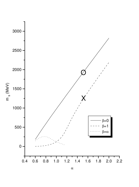
Figure 1: The scalar meson mass as a function of $\alpha$ for different values of $\beta$. The circle and the cross stand for the ZM and ZM3 results respectively.

We will analyze our model in the region $\alpha>1/2$ and for three choices of $\beta$: $\beta=0$, $\beta=1$ and $\beta=\alpha$. The values of $C_{v}^{2}$ and $C_{\sigma}^{2}$ are fixed to reproduce the energy per nucleon $E/N=-15.75$ MeV at $k_{F}=1.3$ fm^-1. Since $g_{\pi}$ is fixed at its experimental value, different values of $C_{\sigma}^{2}$ are related with different values of $m_{s}$. In Fig.1 we show the value of the scalar meson mass obtained from $C_{\sigma}^{2}$ that saturates the nuclear matter, as a function of $\alpha$. The particular results obtained in the ZM and ZM3 models are assigned in this figure by a circle and a cross respectively. From this figure we can see that the choice $\beta=\alpha$ provides very smaller values for $m_{s}$ and delimits the region where the symmetric scaling ($\alpha=\beta$) is valid. If one thinks about finite systems, $m_{s}$ is associated with the range of the scalar interaction. Therefore, smaller values of $m_{s}$ provide longer ranges of the interaction in the configuration space.

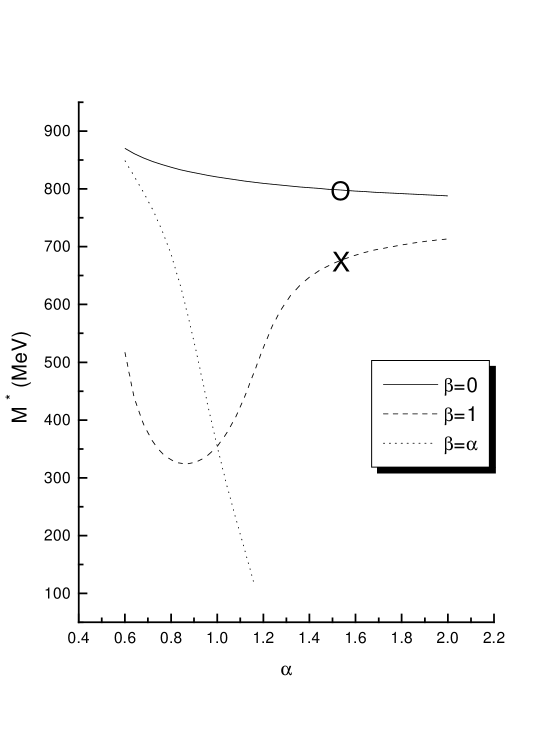
Figure 2: The effective nucleon mass at saturation density as a function of $\alpha$ for different values of $\beta$. The circle and the cross stand for the ZM and ZM3 results respectively.

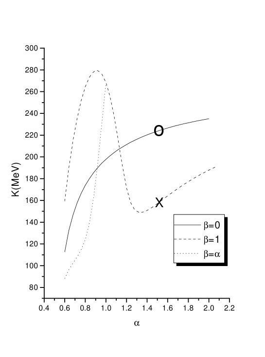
Figure 3: The incompressibility as a function of $\alpha$ for different values of $\beta$. The circle and the cross stand for the ZM and ZM3 results respectively.

In Figs.2 and 3 we show the effective nucleon mass at saturation density, $M_{0}^{*}$, and the incompressibility, $K$, as a function of $\alpha$. As we can see by these figures, a large region of values for $K$ and $M_{0}^{*}$ can be generated by these models and we can choose the values of $\alpha$ and $\beta$ that can better reproduce the phenomenology. It is also interesting to notice that the values generated for the incompressibility by these models are generally small, as compared with QHD for instance.

There is a strong correlation in relativistic models between the effective nucleon mass at saturation density, $M_{0}^{*}$, and the strenght of the spin orbit force in nuclei [16, 17, 18]. Typical values of $M_{0}^{*}/M$ in successful models are roughly 0.6, which yield spin-orbit splittings close to experimental values. Accurate reproductions of observables in finite nuclei, including the spin-orbit splitting in particular, tightly constrain the value of $M_{0}^{*}/M$ in the range $0.58\leq M_{0}^{*}/M\leq 0.70$ [18]. Since in linear chiral models in general $M_{0}^{*}/M$ is too close to unity, this was found as one of the reasons for the failure of the models considered in ref.[4] to give a good description of finite nuclei. As can be seen by figure 2, allowing the coupling constants to decrease with the density we can generate a linear chiral model which gives $M_{0}^{*}/M$ in good agreement with phenomenology. We can also see that the choice $\beta=0$ does not go in this direction generating $M_{0}^{*}/M$ very close to unity, indicating its almost non-relativistic character. The choice $\alpha=\beta$ and $\beta=1$ (for $\alpha$ around 1.5 (ZM3)) seems to be a good candidate.

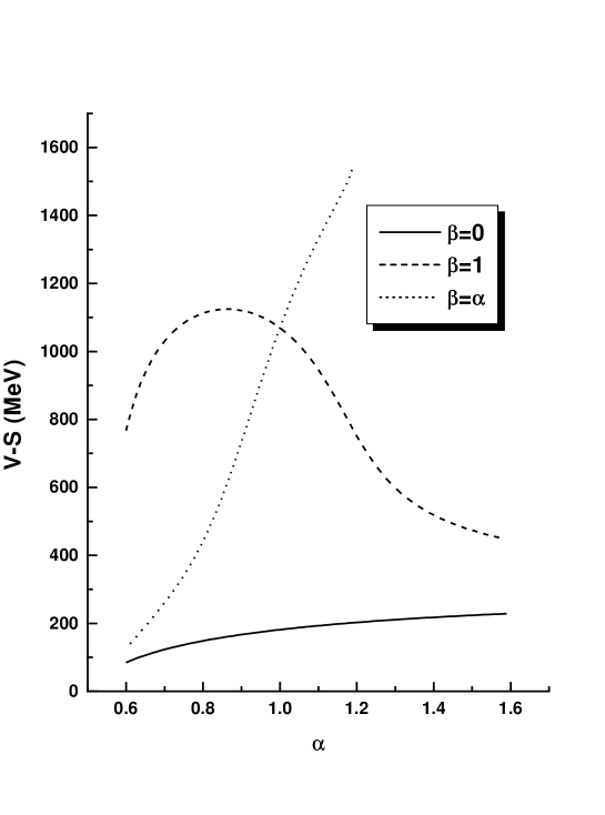
Figure 4: $V-S$ as a function of $\alpha$ for different values of $\beta$.

Another qualitative ingredient associated with the spin-orbit splitting in finite nuclei is the difference between the depth of the vector and scalar potencials, $V-S$ ($S=M^{*}-M$, $V={g_{v}^{*}}^{2}\rho_{B}/m_{v}^{2}$). The higher the difference the higher the splitting. In Fig. 4 we present the difference $V-S$ as a function of $\alpha$. Typical values of this quantity, that give reasonable values for the spin-orbit splitting, lies usually in the region from 550 to 650 MeV [6]. In our models this region can be obtained for the cases $\alpha=\beta$ and $\beta=1$ in agreement with the analysis done above. Of course this is only an indication that good results can be obtained for finite nuclei. A calculation for finite nuclei with these models is under way [20].

To summarize, we have proposed a new class of models for nuclear systems where chiral symmetry is implemented in a linear realization. No new degress of freedom or new interactions other than that present in the original linear-$\sigma$ model [1, 21] were needed. In these models loops are not an essential ingredient to obtain saturation of nuclear matter as in refs.[21, 15]. We found that this class of models reproduces very well the expected saturation properties of nuclear matter. In a mean field approximation and for some particular values of the parameters, these models can reproduce the well known derivative coupling ZM models and QHD. Therefore ZM models and QHD can also be understood as reminiscents of linear chiral models with couplings given by Eqs. (2) and (3), after a mean field approximation and proper choice of $\alpha$ and $\beta$. Let’s remark that ZM models have a desirable nonrelativistic limit in the saturation mechanism. We are aware that for finite nuclei, surface terms can not be neglected and the results for nuclei spectra may differ from the original models [12]. Finally we would like to point out that to the best of our knowledg it is the first time that this class of linear chiral models can reproduce well nuclear matter phenomenology.

ACKNOWLEDGEMENTS

This work was partially supported by FAPESP and CNPq – Brazil.

References

- [1] M. Gell-Mann and M. Lévy, Nuovo Cimento 16, 705 (1960).
- [2] B.D. Serot and J. D. Walecka, Adv. Nucl. Phys. 16, 1 (1986); B.D. Serot, Rep. Prog. Phys. 55, 1855 (1992).
- [3] J. Boguta, Phys. Lett. B120, 34 (1983); B128, 19 (1983).
- [4] R.J. Furnstahl and B.D. Serot, Phys. Rev. C47, 2338 (1993);Phys. Lett. B316, 12 (1993).
- [5] J. L. Friar, Few-Boby Systems Suppl. 99 (1996) 1 and references therein.
- [6] R.J. Furnstahl, H.B. Tang and B.D. Serot, Phys. Rev. C52, 1368 (1995); R.J. Furnstahl, B.D. Serot and H.B. Tang, Nucl. Phys. A615, 441 (1997).
- [7] V.N. Fomenko et al., J. Phys. G 21 , 53 (1995).
- [8] E.K. Heide, S. Rudaz and P.J. Ellis, Nucl. Phys. A571, 713 (1994); P.J. Ellis, E.K. Heide and S. Rudaz, Phys. Lett. B282, 271 (1992).
- [9] K. Saito and A.W. Thomas, Phys. Lett. B327, 9 (1994); K. Saito, K. Tsushima and A.W. Thomas, Nucl. Phys. A609, 339 (1996).
- [10] M.K. Banerjee and J.A. Tjon, Phys. Rev. C56, 497 (1997).
- [11] K. Miyazaki, Prog. Theor. Phys. 91 1271 (1994).
- [12] A. Delfino, M. Chiapparini, M. Malheiro, L.V. Belvedere and A.O. Gattone, Z. Phys. A355, 145 (1996); M. Chiapparini, A. Delfino, M. Malheiro and A.O. Gattone, Z. Phys. A357, 47 (1997).
- [13] J. Zimanyi and S.A. Moszkowski, Phys. Rev. C42, 1416 (1990).
- [14] A. Delfino, C.T. Coelho and M. Malheiro, Phys. Lett. B345, 361 (1995); Phys. Rev. C51, 2188 (1995);
- [15] W. Bentz, L.G. Liu and A. Arima, Ann. Phys. (N.Y.) 188, 61 (1988) ; L.G. Liu, W. Bentz and A. Arima, Ann. Phys. (N.Y.)194, 387 (1989).
- [16] P.-G. Reinhard, Rep. Prog. Phys. 52, 439 (1989).
- [17] A.R. Bodmer, Nucl. Phys. A526, 703 (1991).
- [18] R.J. Furnstahl, J.J. Rusnak and B.D. Serot, Nucl. Phys. A632, 607 (1998).
- [19] C. Callan, S. Coleman, J. Wess and B. Zumino, Phys. Rev. 177, 2247 (1969).
- [20] M. Chiapparini, A. Delfino, F. S. Navarra, M. Nielsen, work in progress.
- [21] T. Matsui and B.D. Serot, Ann. Phys. 144, 107 (1982).