TPR-98-16

Fine-Tuning Two-Particle Interferometry
II: Opacity Effects

Boris Tomášik and Ulrich Heinz

Institut für Theoretische Physik, Universität Regensburg,
D-93040 Regensburg, Germany

May 7, 1998

We present a model study of single-particle spectra and two-particle Bose-Einstein correlations for opaque sources. We study the transverse mass dependence of the correlation radii $R_{\perp}$, $R_{\parallel}$ and $R_{0}$ in the YKP parametrization and find a strong sensitivity of the temporal radius parameter $R_{0}^{2}$ to the source opacity. A simple comparison with the published data from 158 $A$ GeV/$c$ Pb+Pb collisions at CERN indicates that the pion source created in these collisions emits particles from the whole reaction volume and is not opaque. For opaque sources we find certain regions of inapplicability of the YKP parametrization which can be avoided by a slightly different parametrization for the correlator. The physical meaning of the modified parameters is briefly discussed.

1 Introduction

Bose-Einstein correlations in the two-particle momentum spectra of identical particle pairs provide a powerful tool to obtain information about the space-time structure of the particle emitting source. In a previous paper [1] (referred to in the following as “Paper I”) we began a detailed numerical model study of two-particle Bose-Einstein correlations for ultrarelativistic heavy ion collisions. We showed that collective expansion and temperature gradients lead to an $M_{\perp}$ dependence of the correlation radii, and that by studying this dependence one can reconstruct the dynamical state of the collision fireball at freeze-out.

A different feature of the particle source which can also cause observable effects in the $M_{\perp}$ dependence of the correlation radii but was not touched upon in Paper I is the source “opacity” [2, 3]. This mechanism, which could affect the geometric and dynamical interpretation of the correlation radii, will be investigated here.

“Opaque” sources emit particles from a thin shell near the fireball surface and are thus characterized by a smaller spatial extension of the emission zone in the “outward” ($x$) than in the “sideward” ($y$) direction: $\langle\tilde{x}^{2}-\tilde{y}^{2}\rangle<0$. This is true in particular [4] for emission functions from hydrodynamical simulations where freeze-out is implemented along a sharp hypersurface, characterized e.g. by a constant freeze-out temperature. Transparent sources of the type studied, for example, in [5, 6, 7], on the other hand, feature a positive and generally small difference $\langle\tilde{x}^{2}-\tilde{y}^{2}\rangle$ [7].

In Refs. [2, 3] it was pointed out that this feature of opaque sources generally leads to smaller values for $R_{o}$ than for $R_{s}$ in the Cartesian parametrization of the correlator. In particular for pairs with vanishing transverse momentum $K_{\perp}=0$, one has [8] $R_{s}^{2}=\langle\tilde{y}^{2}\rangle>R_{o}^{2}=\langle\tilde{x}^{2}\rangle$ if $\langle\tilde{x}^{2}-\tilde{y}^{2}\rangle<0$. The existence of a thin emission layer with directed emission only into the outward hemisphere thus breaks the usual symmetry argument [6, 9] that $\lim_{K_{\perp}\to 0}(R_{o}^{2}-R_{s}^{2})=0$. That argument is based on the assumed azimuthal symmetry of the effective source for vanishing $K_{\perp}$ where the direction of the transverse pair momentum no longer serves to distinguish between the outward and sideward directions (parallel and perpendicular to $\bf{K}_{\perp}$); for opaque sources the orientation of the emitting surface itself provides that distinction.

Here we show that in the Yano-Koonin-Podgoretskiĭ (YKP) parametrization [6, 10] the opacity effects get enhanced in the “temporal” radius parameter $R_{0}^{2}$ which turns negative for small $K_{\perp}$ and diverges to minus infinity in the limit $K_{\perp}\to 0$ if $\langle\tilde{x}^{2}-\tilde{y}^{2}\rangle<0$. While this would destroy the interpretation of $R_{0}$ in terms of an effective source lifetime, it would provide particularly clear evidence for surface dominated emission. Since no such evidence is seen in the data from the NA49 Collaboration [11, 12], rather stringent limits on the degree of “opaqueness” of the source created in these collisions can already now be established (see Sec. 3.3).

In the course of this study we discovered that for opaque sources the YKP parametrization may become ill-defined in certain kinematic regions. In Sec. 4.2 we introduce a modification of the YKP parametrization without this defect. The cost for the remedy is a less straightforward physical interpretation of its radius parameters. Fortunately, for transparent sources the YKP parametrization with its simpler space-time interpretation generally appears to work well.

For the general formalism and notation we refer the reader to Paper I. In the next Section we introduce the modification of the emission function from Paper I which is needed to parametrize the opacity of the source. In Sec. 3 we describe the results of our model study. Some problems with the YKP parametrization for opaque sources are discussed and corrected in Sec. 4, and the results are summarized in Sec. 5. As in Paper I we consider only directly emitted pions from the thermalized source, neglecting pions from resonance decays whose effects were studied in Refs. [13].

2 A model for opaque sources

Following the idea of Heiselberg and Vischer [2, 3] we introduce the opacity into the model emission function from Paper I via an additional exponential factor $\exp[-\l_{\rm eff}/\lambda]$ which suppresses the emission of the particles from deep inside the source. $l_{\rm eff}(r,\phi)$ is the effective length which a particle emitted at point $(r,\varphi)$ travels in outward ($x$) direction before leaving the source. We implement the Gaussian transverse density profile as follows:

$$l_{\rm eff}(r,\phi)=e^{-\frac{y^{2}}{2R^{2}}}\,\int_{x}^{\infty}\,e^{-\frac{{x^{\prime}}^{2}}{2R^{2}}}\,dx^{\prime}\qquad{\rm with}\quad y=r\,\sin\phi,\>x=r\,\cos\phi\,.$$ (1)

$\lambda$ represents the specific mean free path of the particle in the medium. The actual mean free path would be obtained by dividing $\lambda$ by the medium density; this is, however, already included in Eq. (1). In the limit $\lambda\to\infty$ the transparent source of Paper I is recovered. Note that, in contrast to [3], our mean free path $\lambda$ and transverse geometric radius $R$ are time-independent. For later convenience we introduce the opacity parameter

$$\omega={R\over\lambda}\,.$$ (2)

Transparent sources are characterized by $\omega=0$.

The complete emission function now becomes

$$S(x,K)\,d^{4}x \propto {M_{\perp}\cosh(\eta-Y)\over(2\pi)^{3}}\;\exp\left[-\frac{K\cdot u(x)}{T}\right]\;\exp\left[-{r^{2}\over 2R^{2}}-{{(\eta-\eta_{0})}^{2}\over 2(\Delta\eta)^{2}}\right]$$ (3)

$$\times\exp\left[-\frac{l_{\rm eff}}{\lambda}\right]\;\frac{\tau\,d\tau}{\sqrt{2\pi(\Delta\tau)^{2}}}\exp\left[-{(\tau-\tau_{0})^{2}\over 2(\Delta\tau)^{2}}\right]\,d\eta\,r\,dr\,d\phi.$$

We do not specify the normalization of the emission function; in principle it is fixed by the total number of produced particles. For the shape of the single-particle spectra and two-particle correlations the normalization is irrelevant. As we will see a meaningful comparison with data is possible even without knowing the normalization of the emission function and permits us to exclude a large class of opaque source models.

The collective flow velocity profile $u(x)$ is parameterized as in Paper I. We will deviate from the discussion presented there by assuming a constant freeze-out temperature $T$.

3 One- and two-particle spectra from opaque sources

In this Section we show and discuss the results of numerical calculations of correlation radii from the emission function (3). All calculations are based on the model-independent expressions which give the correlation radii in terms of space-time variances of the emission function. For the Cartesian parametrization of the correlator they read [8, 14, 15]

$$R_{s}^{2}({\bf K}) = \langle\tilde{y}^{2}\rangle\,,$$ (4)

$$R_{o}^{2}({\bf K}) = \langle(\tilde{x}-\beta_{\perp}\tilde{t})^{2}\rangle\,,$$ (5)

$$R_{l}^{2}({\bf K}) = \langle(\tilde{z}-\beta_{l}\tilde{t})^{2}\rangle\,,$$ (6)

$$R_{ol}^{2}({\bf K}) = \langle(\tilde{x}-\beta_{\perp}\tilde{t})(\tilde{z}-\beta_{l}\tilde{t})\rangle\,,$$ (7)

where $\tilde{x}_{\mu}=x_{\mu}-\langle x_{\mu}\rangle$ and $\langle\cdots\rangle$ denotes the space-time average taken with the emission function (see Paper I). For the YKP parametrization radii we have [7, 10]

$$v({\bf K}) = {A+B\over 2C}\left(1-\sqrt{1-\left({2C\over A+B}\right)^{2}}\right)\,,$$ (8)

$$R_{\parallel}^{2}({\bf K}) = B-v\,C\,,$$ (9)

$$R_{0}^{2}({\bf K}) = A-v\,C\,,$$ (10)

$$R_{\perp}^{2}({\bf K}) = {\langle{\tilde{y}^{2}}\rangle}\,,$$ (11)

where

$$A = \langle\tilde{t}^{2}\rangle-\frac{2}{\beta_{\perp}}\langle\tilde{t}\tilde{x}\rangle+\frac{1}{\beta^{2}_{\perp}}\langle\tilde{x}^{2}-\tilde{y}^{2}\rangle\,,$$ (12)

$$B = \langle\tilde{z}^{2}\rangle-2\frac{\beta_{l}}{\beta_{\perp}}\langle\tilde{z}\tilde{x}\rangle+\frac{\beta_{l}^{2}}{\beta^{2}_{\perp}}\langle\tilde{x}^{2}-\tilde{y}^{2}\rangle\,,$$ (13)

$$C = \langle\tilde{z}\tilde{t}\rangle-\frac{\beta_{l}}{\beta_{\perp}}\langle\tilde{t}\tilde{x}\rangle-\frac{1}{\beta_{\perp}}\langle\tilde{z}\tilde{x}\rangle+\frac{\beta_{l}}{\beta^{2}_{\perp}}\langle\tilde{x}^{2}-\tilde{y}^{2}\rangle\,.$$ (14)

In the following subsection we study the basic opacity effects on the one- and two-particle spectra. Some of these are analyzed in more detail in subsection 3.2. A comparison with available data is presented in subsection 3.3.

3.1 Basic opacity effects

The basic free parameter of our study is the mean free path $\lambda$. We will scan a rather wide range of opacities $\omega=R/\lambda$ ($\omega=0,\,1,\,10$). For $\eta_{f}$, which parametrizes the transverse flow at freeze-out linearly according to

$$\eta(r)=\eta_{f}\left({r\over R}\right)\,,$$ (15)

we will study two different values, $\eta_{f}=0$ (a source without transverse flow) and $\eta_{f}=0.5$ (rather strong transverse flow). All other model parameters are kept fixed in this and the following subsection at the values listed in Table 1 which are motivated by the SPS Pb+Pb data (see Sec. 3.3).

Table 1: Model parameter values used in the calculations of Sec. 3.1.

temperature $T$	120 MeV
average freeze-out proper time $\tau_{0}$	8 fm/$c$
mean proper emission duration $\Delta\tau$	2 fm/$c$
geometric (Gaussian) transverse radius $R$	6.5 fm
Gaussian width of the space-time rapidity profile $\Delta\eta$	1.3
pion mass $m_{\pi^{\pm}}$	139 MeV/$c^{2}$

The calculations in this and the following subsection are done for pions and pion pairs at midrapidity ($Y_{{}_{\rm CM}}\equiv Y_{\pi\pi}-Y_{{}_{\rm CMS}}=0$).

To obtain an impression of how the source changes when varying $\omega$ and $\eta_{f}$ we show in Fig. 1 for pions with transverse momentum $K_{\perp}=400$ MeV/$c$ transverse cuts of the effective emission function, $S(x,y;K_{\perp}=400\,{\rm MeV}/c)$, as contour plots.

Figure 1: Transverse cuts of the emission function for midrapidity pions with transverse momentum $K_{\perp}=400$ MeV/$c$ (in $x$-direction), for the model parameters given in Table 1. Top row: no transverse flow ($\eta_{f}=0$), bottom row: transverse flow with $\eta_{f}=0.5$. The columns correspond to different opacities: $\omega=0$ (left), $\omega=1$ (middle), $\omega=10$ (right).

When switching on the opaqueness, the “transverse” size (in y- or side-direction) of the effective source is seen to increase dramatically (cf. Figs. 1a-c); this is due to the suppression factor $\exp[-l_{\rm eff}/\lambda]$ which cuts out all of the interior of the source and leaves only the right hemisphere of the dilute tail of the Gaussian transverse density distribution. This cannot happen in the model of Heiselberg and Vischer [2] who use a transverse box profile without Gaussian tails. For a source with the shape given in Fig. 1c the Gaussian approximation, on which the model-independent expressions from the beginning of this Section are based, may become questionable; for a qualitative understanding of the relevant features it should, however, be sufficient.

Transverse flow (lower row in Fig. 1) is seen to decrease the effective source more in the sideward than in the outward direction; this effect is the stronger the larger the opacity $\omega$.

The single-particle transverse mass spectra resulting from these models are shown in Fig. 2.

Figure 2: Comparison of $m_{\perp}$ spectra for transparent and opaque sources at midrapidity. For the model parameters see Table 1. Thin lines correspond to models without transverse flow, thick lines to models with $\eta_{f}=0.5$. For reference, solid lines represent the spectra of the transparent model ($\omega=0$). Dashed and dotted lines show the spectra from sources with $\omega=1$ and $\omega=10$ respectively.

The normalization of the spectra is arbitrary since the emission function was not normalized. The interesting information is carried by the spectral slopes. For non-expanding sources, the slopes for opaque and transparent sources are identical. For expanding sources with fixed $\eta_{f}$, an opaque source yields much flatter spectra than a transparent source. The reason is obvious from Fig. 1: due to the opacity much stronger weight is given to the rapidly expanding surface than to the less rapidly expanding interior regions. This implies that the average flow velocity $\langle v_{\perp}\rangle$ is larger for the opaque source. In [16] it was argued that (for $m_{\perp}\gg m_{0}$) the slope of the $m_{\perp}$-spectrum is given approximately by the blue-shifted temperature

$$T_{\rm eff}\approx T\sqrt{\frac{1+\langle v_{\perp}\rangle}{1-\langle v_{\perp}\rangle}}\,.$$ (16)

We should therefore expect roughly the same slopes if with increasing opacity $\omega$ the flow parameter $\eta_{f}$ were reduced to keep $\langle v_{\perp}\rangle$ fixed. In subsection 3.3 we will show how this works.

The two-particle correlations resulting from these models are studied in Fig. 3.

Figure 3: Comparison of correlation radii from transparent and opaque sources for pion pairs with rapidity $Y_{{}_{\rm CM}}=0$. The source parameters are given in Table 1. Thin lines: $\eta_{f}=0$, thick lines: $\eta_{f}=0.5$. Solid lines: $\omega=0$ (transparent source), dashed lines: $\omega=1$, dotted lines: $\omega=10$. Note that $R_{s}=R_{\perp}$ and for $Y_{{}_{\rm CM}}=0$ the longitudinal correlation radius $R_{l}=R_{\parallel}$ and $Y_{{}_{\rm YK}}=0$ in LCMS.

For midrapidity pions the cross-term $R_{ol}$ in the Cartesian parametrization (7) and the Yano-Koonin velocity $v$ of the YKP parametrization (8) vanish, and $R_{l}=R_{\parallel}$. Furthermore, $R_{s}=R_{\perp}$ in general.

Surprisingly, without transverse flow the outward radius decreases only weakly with increasing opacity. This is a specific feature of our Gaussian parametrization of the source geometry and not true for a box profile as studied by Heiselberg and Vischer [2, 3]. In their case no emission from regions outside the box radius $R$ is possible, and opacity leads to an effective emission function which is “squeezed” into a very thin crescent-shaped region close to the edge of the box. In our parametrization, increasing opacity favors emission from the more dilute tail of the Gaussian density distribution, and as $\omega$ increases the effective emission region just moves further outward, becoming part of a shell with a radius $R_{\rm shell}>R$ whose thickness happens to be more or less independent of $\omega$. The sideward homogeneity radius $R_{s}$, on the other hand, grows with $R_{\rm shell}$ as seen in the top row of Fig. 1 and thus increases dramatically with increasing opacity.

For transparent sources it is well known that transverse flow causes a reduction of the sideward and outward homogeneity regions $\langle\tilde{y}^{2}\rangle$ and $\langle\tilde{x}^{2}\rangle$, respectively, the more so the larger $M_{\perp}$ [5, 9, 15, 17]. For fixed transverse flow parameter $\eta_{f}$, this effect is seen to be even stronger for opaque sources, reflecting again the growing average transverse flow velocity with increasing $\omega$. The right upper panel of Fig. 3 shows that for very opaque sources this effect even eliminates the slight initial rise of $R_{o}$ for small $K_{\perp}$: the decrease of $\langle\tilde{x}^{2}\rangle$ with transverse mass is then stronger than the increasing contribution from the term $\beta^{2}_{\perp}\langle\tilde{t}^{2}\rangle$ in (5).

It has been proposed in [2] to identify opaque sources by looking for a negative difference $R_{o}^{2}-R_{s}^{2}$, especially at $K_{\perp}\approx 0$. In the lower left panel of Fig. 3 we show that much more dramatic opacity effects are seen in the “temporal” YKP parameter $R_{0}^{2}$. For midrapidity pion pairs $R_{0}^{2}$ is given in the CMS frame (which is also the rest frame of the emitting fluid element where $v({\bf K})$ is zero) by

$$R_{0}^{2}=\langle{\tilde{t}}^{2}\rangle-\frac{2}{\beta_{\perp}}\langle\tilde{x}\tilde{t}\rangle+\frac{1}{\beta_{\perp}^{2}}\langle{\tilde{x}}^{2}-{\tilde{y}}^{2}\rangle\,.$$ (17)

For opaque sources the last term on the r.h.s. is negative and diverges to $-\infty$ as $K_{\perp}\to 0\;(\beta_{\perp}\to 0)$. Transverse flow reduces this negative contribution, but not sufficiently to reverse the overall negative sign of $R_{0}^{2}$ in the region of small $K_{\perp}$. As seen in Fig. 3 this specific feature of opaque sources is quite stable against a reduction of the opacity $\omega$ in the sense that it even shows for nearly transparent sources with $\omega=1$ at sufficiently large $K_{\perp}$-values to be measurable.

Compared to $R_{s}$, $R_{o}$, and $R_{0}$, the opacity effects on $R_{l}=R_{\parallel}$ (shown in the lower right panel of Fig. 3) are weak. They can all be explained in terms of the different values for the average transverse flow velocities in the studied examples as discussed in Paper I.

3.2 A more detailed discussion of $R_{o}^{2}-R_{s}^{2}$ and $R_{0}^{2}$

The interesting opacity effects on $R_{o}^{2}-R_{s}^{2}$ and on $R_{0}^{2}$ deserve a more detailed discussion. To this end we plot in Fig. 4

Figure 4: Opacity effects on $R_{o}^{2}-R_{s}^{2}$ (left column) and $R_{0}^{2}$ (right column). The solid lines show the radius parameters as they enter the correlation function, the other lines show how they are decomposed into contributions from various space-time variances. Left column: the dashed line shows $\beta^{2}_{\perp}\langle\tilde{t}^{2}\rangle$, the dotted line $-2\beta_{\perp}\langle\tilde{x}\tilde{t}\rangle$, and the dash-dotted line $\langle\tilde{x}^{2}-\tilde{y}^{2}\rangle$. In the right column the same symbols denote the same quantities divided by $\beta_{\perp}^{2}$. All curves are calculated at $Y_{{}_{\rm CM}}=0$, with model parameters from Table 1 except for $R=7$ fm and $\eta_{f}=0.3$. Upper row: $\omega=0$ (transparent source); lower row: $\omega=10$ (opaque source).

the various contributions to these radius parameters from the space-time variances of a transparent (upper row) and an opaque source (lower row), both for the standard Cartesian (left column) and YKP parametrizations (right column). We show results for moderate transverse flow $\eta_{f}=0.3$ and midrapidity pion pairs, but we checked that no qualitative differences occur for forward rapidities. The diagrams in Fig. 4 can be concisely summarized by stating that for transparent sources the lifetime term $\langle\tilde{t}^{2}\rangle$ dominates the difference $R_{o}^{2}-R_{s}^{2}$ and $R_{0}^{2}$ (at least for small $K_{\perp}$) while for opaque sources the difference $\langle\tilde{x}^{2}-\tilde{y}^{2}\rangle$ of transverse spatial variances takes the leading role.

These results confirm the conclusion of Ref. [2] that, within the Cartesian parametrization, opaque sources generically lead to negative values for the difference $R_{o}^{2}-R_{s}^{2}$. Our calculations were done in the Yano-Koonin ($v=0$) frame, and we checked that in this frame this qualitative conclusion is independent of the pair rapidity. In the YKP parametrization the same feature appears strongly enhanced in the parameter $R_{0}^{2}$, especially at small values of $K_{\perp}$, due to the division of the relevant combination of space-time variances by the factor $\beta_{\perp}^{2}$. A negative value for $R_{0}^{2}$ corresponds to a negative value for $R_{o}^{2}-R_{s}^{2}$ in the Yano-Koonin frame (which is usually not much different from the LCMS [7]).

3.3 Comparison with data

In this subsection we compare the model calculations with recently published correlation data from 158 GeV/$c$ Pb+Pb collisions at the SPS [11], focusing on opacity effects. To constrain the model parameters we make use also of preliminary data on single-particle spectra [12, 18].

When we increase the opacity without changing any of the other model parameters we obtain a larger transverse HBT radius $R_{\perp}$ since the opacity factor favors particle emission from the dilute tail of the transverse Gaussian density distribution. In order to reproduce a fixed measured value for $R_{\perp}$ with sources of increasing opacity we must therefore reduce the Gaussian width parameter $R$ in the emission function.

By the same mechanism larger opacities lead, at fixed $\eta_{f}$, to larger average transverse flow velocities in the source. These cause a flatter slope of the single-particle $m_{\perp}$-spectrum (Fig. 2) and a steeper $M_{\perp}$-dependence of the transverse HBT radius $R_{\perp}$ (Fig. 3). On a qualitative level both effects can be studied analytically: for pions the inverse slope parameter of the single-particle $m_{\perp}$-spectrum is given by Eq. (16), while the $M_{\perp}$-dependence of $R_{\perp}$ is approximately given by [6, 15]

$$R_{\perp}^{2}\approx{R^{2}\over 1+\left({M_{\perp}\over T}\right)\langle v_{\perp}\rangle^{2}}\,.$$ (18)

This expression is derived from Eq. (11) by evaluating the average $\langle\tilde{y}^{2}\rangle$ over the emission function via saddle point integration [6, 15]. Although not quantitatively reliable [9], it illustrates nicely an important point [19, 20, 21, 11, 12]: while (16) and (18) are, each by itself, ambiguous and do not allow to separate $T$ and $\langle v_{\perp}\rangle$, the correlation between those two parameters is opposite in the two equations. By combining them the collective transverse flow $\langle v_{\perp}\rangle$ can be isolated from the random thermal motion $\sim T$. The value for $T$ given in Table 1 stems from a rough numerical fit [21] to the measured single-particle spectra and correlation radii from Pb+Pb collisions at the SPS [11, 18]. We expect it to be accurate to about $\pm 10$ MeV.

Once $T$ is known, the average transverse flow is fixed by the slope of the single-pion transverse mass spectrum. For $T=120$ MeV the NA49 spectra [18] yield an average transverse flow velocity $\langle v_{\perp}\rangle\simeq 0.4c-0.45c$ [22, 20, 21]. For our source model the average transverse flow velocity is given by ($\xi=r/R$)

$$\langle v_{\perp}\rangle = {1\over NR^{2}}\int_{0}^{\infty}r\,dr\int_{0}^{2\pi}d\phi\,v_{\perp}(r)\,\exp\left(-\frac{r^{2}}{2\,R^{2}}\right)\,\exp\left(-\frac{l_{\rm eff}(r,\phi)}{\lambda}\right)$$

$$= \frac{1}{N}\int_{0}^{\infty}\xi\,d\xi\Biggl{[}\tanh\left(\eta_{f}\xi\right)\,e^{-{\xi^{2}\over 2}}\,\int_{0}^{2\pi}d\phi\,\exp\left(-\omega\,e^{-{\xi^{2}\sin^{2}\phi\over 2}}\int_{\xi\cos\phi}^{\infty}e^{-{\zeta^{2}\over 2}}d\zeta\right)\Biggr{]}\,;$$

$$N = \int_{0}^{\infty}\xi\,d\xi\left[e^{-{\xi^{2}\over 2}}\int_{0}^{2\pi}d\phi\,\exp\left(-\omega\,e^{-{\xi^{2}\sin^{2}\phi\over 2}}\,\int_{\xi\cos\phi}^{\infty}e^{-{\zeta^{2}\over 2}}d\zeta\right)\right]\,.$$

This equation implies that, for fixed $\langle v_{\perp}\rangle$, $\eta_{f}$ must be reduced if $\omega$ is increased. Therefore, if we want to keep the absolute value of $R_{\perp}$, its $M_{\perp}$ slope, and the slope of the single-particle $m_{\perp}$-spectrum fixed, we must decrease both $R$ and $\eta_{f}$ as we increase the opacity $\omega$.

Three models with opacities $\omega=0,\,1,\,10$ were studied and compared with the data. In each case we tuned $\eta_{f}$ such that $\langle v_{\perp}\rangle=0.44$ was kept fixed, and we adjusted $R$ such that the size of $R_{\perp}(M_{\perp})$ is roughly reproduced. This choice was motivated by the NA49 data shown in the right column of Fig. 4 of Ref. [11] (HBT radii from 158 GeV/$c$ Pb+Pb collisions, $h^{-}h^{-}$ correlations in the rapidity window $3.9<Y_{\pi\pi}<4.4$). The values of $R$ and $\eta_{f}$ used in these calculations are listed in Table 2.

Table 2: Transverse flow strength $\eta_{f}$ and Gaussian radius $R$ for the three models which are used in the comparison with the data in Sec. 3.3.

$\omega$ (opacity)	$\eta_{f}$	$R$
0 (transparent)	0.4	5.74 fm
1	0.345	4.83 fm
10 (opaque)	0.215	3.35 fm

To fit the parallel correlation radius $R_{\parallel}$ (see later) the average freeze-out time $\tau_{0}$ has been set to 6.1 fm. Other model parameters are taken from Table 1.

In Fig. 5

Figure 5: Single-particle $m_{\perp}$-spectra from the models listed in Table 2. Solid, dashed, and dotted lines correspond to models with $\omega=0,\,1,\,10$, respectively. The thin dash-dotted auxiliary lines show a straight exponential with inverse slope $T_{\rm eff}=T\sqrt{(1+\langle v_{\perp}\rangle)/(1-\langle v_{\perp}\rangle)}$, for $T=120$ MeV and $\langle v_{\perp}\rangle=0.44$ resp. $\langle v_{\perp}\rangle=0.49$. The spectra are computed at midrapidity where the analysis of [22] was performed.

we plot the single-particle $m_{\perp}$-spectra resulting from these models. (Recall that only the slopes, but not the normalization are relevant here.) According to Eq. (16) we expect the same slopes for all spectra, which should be characterized by the blue-shifted temperature with $\langle v_{\perp}\rangle=0.44$. This is roughly borne out by the calculation, but for transparent and mildly opaque sources the spectra are visibly concave [16] and show an increasingly flatter slope for $m_{\perp}>1$ GeV. The reason for this is well-known [16]: for large $m_{\perp}$ the spectra are dominated not by particles from fluid cells with the average transverse flow velocity $\langle v_{\perp}\rangle$, but from more rapidly moving fluid cells in the tail of the transverse density profile. This detail cannot be accurately accounted for by the simple formula (16). In other words: for a specified $p_{\perp}$ there is only a part of the source contributing to the particle production – this is the effective source for that $p_{\perp}$. The slope of the spectra at that value of $p_{\perp}$ is given by the blue-shifted temperature where the average transverse expansion velocity is to be calculated over the effective source. For the very opaque source this average velocity is (accidentally) independent of $p_{\perp}$, and the spectrum is thus exactly exponential. However, to reproduce its slope via (16) we need $\langle v_{\perp}\rangle=0.49$, a somewhat larger value than the average transverse expansion velocity computed over the complete source. Note that the experimental spectra resemble more the concave spectrum of the transparent source than the straight line originating from the opaque one.

Fig. 6 shows

Figure 6: $M_{\perp}$ dependences of the YKP correlation radii at $Y_{{}_{\rm CM}}=1.25$ resulting from the three models in Table 2. (Same line symbols as in Fig. 5.) The data are from 158 $A$ GeV/$c$ Pb+Pb collisions taken by the NA49 collaboration [11].

the corresponding set of YKP correlation radii, evaluated at $Y_{{}_{\rm CM}}=1.25$ where the NA49 collaboration has published the $M_{\perp}$ dependence of the three YKP radius parameters from 158 $A$ GeV/$c$ Pb+Pb collisions at the SPS (Fig. 4 in Ref. [11]). Note that the systematic error of the data, estimated to be $\pm 15\%$ [11], is not included in the plots. In Fig. 6a one sees that by simply adjusting the source parameters to keep the magnitudes of $R_{\perp}$ and $\langle v_{\perp}\rangle$ approximately constant, the $M_{\perp}$-dependence of $R_{\perp}$ is reasonably well reproduced by all three models. This implies that the average transverse flow velocity is indeed the dominating factor for the $M_{\perp}$-slope of the transverse HBT radius. We found that the agreement between model and data can be further improved by additional fine-tuning of the parameters, in particular by taking into account a non-vanishing transverse temperature gradient. Since a fully quantitative analysis requires, however, also the inclusion of resonance decays which may cause an additional $M_{\perp}$ dependence [13, 23], and since the following arguments will not depend on such details we will not enter into this discussion here.

The longitudinal radius parameter $R_{\parallel}$ shows even less sensitivity to the opacity $\omega$ (Fig. 6b). The reason is that it is determined mainly by the values $\tau_{0}$ (average freeze-out proper time) and $\Delta\tau$ (mean emission duration), and its $M_{\perp}$ dependence is dominated by the boost-invariant longitudinal expansion [24, 7]. Since, except for very forward and backward rapidities, opacity affects the emission function mostly in the transverse direction, $R_{\parallel}$ is hardly modified. By appropriately adjusting $\tau_{0}$, the data for $R_{\parallel}$ are very well reproduced. Note that for opaque sources the calculated curves feature a gap at small values of $M_{\perp}$ and behave strangely near $M_{\perp}=m_{\pi}$; the origin of this behaviour will be explained in Sec. 4. This problem does not arise at midrapidity where unpublished data on the $M_{\perp}$-dependence of $R_{\parallel}$ can be found in the PhD theses [25] which we were able to fit equally well all the way down to $K_{\perp}=0$ with our emission function for all three values of $\omega$, using $\tau_{0}=8$ fm/$c$.

Since the space-time rapidity width $\Delta\eta=1.3$ is fixed by the width of the single-particle rapidity distribution [19, 11] and $\tau_{0}$ has been set to the value of 6.3 fm, at this point the emission duration $\Delta\tau$ is the only remaining free parameter in the emission function. For transparent sources ($\omega=0$) it should be fixed by the asymptotic value of $R_{0}$ at large values of $M_{\perp}$ [10]. (Its effects on $R_{\perp}$ are negligible, and for $\Delta\tau\ll\tau_{0}$ they are also small for $R_{\parallel}$ [7].) In Fig. 6c we compare with the data our results for $R_{0}^{2}$ for a fixed value $\Delta\tau=2$ fm/$c$, but for three different opacities. Clear disagreement with the data is seen for the opaque models. Already the still rather transparent model with $\omega=1$ (cf. Fig. 1) misses nearly all data points.

The question arises to which extent this disagreement can be avoided by readjusting the duration of particle emission $\Delta\tau$. As mentioned before and seen in Fig. 6c, for opaque sources the asymptotic value of $R_{0}^{2}$ at large $M_{\perp}$ is no longer given by the effective source lifetime $\langle\tilde{t}^{2}\rangle$ in the YK frame alone, but also receives a strong negative geometric contribution $\langle\tilde{x}^{2}-\tilde{y}^{2}\rangle$ (cf. Eq. (17)). One might try to compensate this effect by increasing for opaque sources the lifetime $\Delta\tau$. This is physically not unreasonable because opaque sources emit particles only from the surface; to produce the same total particle yield the resulting reduced brightness must be compensated by a larger emission duration. However, larger values of $\Delta\tau$ lead also to an increase of $R_{\parallel}$ which must be compensated by reducing the average freeze-out time $\tau_{0}$. Since our model parametrization looses its meaning for $\Delta\tau>\tau_{0}$, there are clear limits to what can be achieved in this way.

In Fig. 7

Figure 7: The YKP radius parameters $R_{0}^{2}$ (a) and $R_{\parallel}$ (b) computed for $\omega=1$ and different values of $\tau_{0}$ and $\Delta\tau$ at $Y_{{}_{\rm CM}}=1.25$. Solid lines: $\tau_{0}=5\,\mbox{fm/}c,\,\Delta\tau=3\,\mbox{fm/}c$; dashed lines: $\tau_{0}=5\,\mbox{fm/}c,\,\Delta\tau=4\,\mbox{fm/}c$; dotted lines: $\tau_{0}=6\,\mbox{fm/}c,\,\Delta\tau=3\,\mbox{fm/}c$; dash-dotted lines: $\tau_{0}=7\,\mbox{fm/}c,\,\Delta\tau=3\,\mbox{fm/}c$. Other model parameters are taken from the corresponding calculation in Fig. 6.

we show $R_{\parallel}$ and $R_{0}^{2}$ for a mildly opaque source with $\omega=1$ for different combinations of $\tau_{0}$ and $\Delta\tau$ and compare them with the data [11]. For $R$ and $\eta_{f}$ we took the corresponding values from Table 2.

One sees that the largest lifetime $\Delta\tau$ compatible with the large-$K_{\perp}$ data for $R_{\parallel}$ is 4 fm/$c$. To maintain a reasonable description of $R_{\parallel}$ in this case $\tau_{0}$ must be reduced to 5 fm/$c$ which brings it dangerously close to $\Delta\tau$. Still, the corresponding curves for $R_{0}^{2}$ all miss the first data points by a large margin. Since however, as already seen in Fig. 6, at the given value of the pair rapidity the calculated curves for $R_{0}^{2}$ feature a gap at low $K_{\perp}$ (indicating that for our model the YKP parametrization is not well-defined in this momentum region, see Sec. 4), one may question the significance of this failure of our model to reproduce the data. For this reason we also checked the behaviour of $R_{0}^{2}$ and $R_{\parallel}$ in different rapidity bins, using the unpublished data of Ref. [25]. In all cases the data points for $R_{0}^{2}$ at the lowest $K_{\perp}$ values are positive, while the calculated curves for opaque sources with $\omega\geq 1$ give strongly negative values, missing the data by far. In particular, this is true at midrapidity where the YKP parametrization remains well-defined down to $K_{\perp}=0$ even for strongly opaque sources.

We conclude that the NA49 data appear to exclude source opacities $\omega>1$, i.e. sources with a “surface thickness” $\lambda<R$. The pion source created in Pb+Pb collisions at the CERN SPS seems to be rather “transparent” at freeze-out, i.e. at the end of the hydrodynamical expansion phase the pions freeze-out in bulk, decoupling essentially everywhere at the same time, including the center of the collision region. It must be kept in mind, however, that this conclusion rests heavily on the positive experimental values for $R_{0}^{2}$ at small $K_{\perp}$ reported by the NA49 collaboration. In [2, 3] it was remarked that preliminary NA44 data from Pb+Pb collisions at the SPS indicate that at small $M_{\perp}$ in the Cartesian parametrization $R_{o}^{2}$ might be smaller than $R_{s}^{2}$ (see [26]); this would favor an opaque source. In our opinion it is premature to draw firm conclusions from these data because, unlike NA49 [11], the NA44 Collaboration has not yet presented a YKP fit of their data, where the opacity signal should be much clearer. Taking their Cartesian fit presented in [26] at face value we conclude that, while a mildly opaque source with $\omega\simeq 1$ cannot be excluded, the NA44 data are also inconsistent with strongly surface dominated emission ($\omega>10$).

In the next Section we will explain the origin of the missing pieces in the curves for $\omega>1$ in Figs. 6 and 7.

4 Modified YKP parametrization

In the previous Section we discovered an intrinsic deficiency of the YKP parametrization which had gone unnoticed before. In this Section we explain the limitations of the YKP parametrization and suggest a slightly different parametrization which avoids these problems and should be particularly suitable for strongly opaque, azimuthally symmetric sources with dominant longitudinal expansion.

4.1 Forward rapidity pion pairs from opaque sources

In Fig. 8

Figure 8: The YKP radii and the Yano-Koonin rapidity in the LCMS for pion pairs with $Y_{{}_{\rm CM}}=1.5$ from an opaque source ($\omega=10$) with $R=4$ fm. Solid lines: $\eta_{f}=0$. Dashed lines: $\eta_{f}=0.6$. The other model parameters are taken from Table 1. The arrows connect the curves across the gap in which the YKP parametrization is not defined.

we show the YKP radius parameters $R_{0}^{2}$ and $R_{\parallel}$ and the YK rapidity $Y_{{}_{\rm YK}}={1\over 2}\ln[(1+v)/(1-v)]$ (relative to the LCMS) for pion pairs at forward rapidity $Y_{{}_{\rm CM}}=1.5$ for opaque sources with and without transverse flow. Let us first discuss the Yano-Koonin rapidity $Y_{{}_{\rm YK}}$: For transparent sources we know from [7, 10] that the YK rapidity is negative in the LCMS, i.e. that the effective source moves somewhat more slowly in the beam direction than the emitted pairs. For opaque sources this seems no longer to be true; for example, in Fig. 8 in the absence of transverse flow the YK rapidity comes out positive in the LCMS. We hasten to stress that this does not imply that in this case the effective source moves faster than the emitted pairs (which would indeed be counterintuitive); it rather reflects the fact that for opaque sources the geometric correction terms in the expression for the YK velocity (see Eq. (4.1) in Ref. [7]), in particular the one proportional to $\langle\tilde{x}^{2}-\tilde{y}^{2}\rangle$, are large and spoil the interpretation of $v$ as the longitudinal source velocity.

Figs. 6 and 8 show that these correction terms can cause even more severe problems: in certain $M_{\perp}$-regions the argument of the square root in (8) turns negative and the YK velocity (and thus also $R_{0}^{2}$ and $R_{\parallel}^{2}$, see (9), (10)) becomes undefined. The conditions for the occurrence of such a pathological behaviour are discussed in Appendix A. It appears that it is connected in a generic way to $\langle\tilde{x}^{2}\rangle<\langle\tilde{y}^{2}\rangle$ which, as we have seen, characterizes opaque sources.

Note that the mentioned “strange” behaviour of the YK velocity, in the regions where it is defined, is reflected via Eqs. (9) and (10) in also unexpected behaviour of $R_{\parallel}$ and $R_{0}^{2}$ especially near to the gap.

4.2 A solution of the problem

This problem of the YKP parametrization can be avoided by a simple technical modification which we call “Modified Yano-Koonin-Podgoretskiĭ” parametrization. It differs from the YKP parametrization by using $q_{s}$ rather than $q_{\perp}=\sqrt{q_{s}^{2}+q_{o}^{2}}$ as one of the three independent components of the relative momentum $q$. For distinction we denote the corresponding HBT parameters with a prime:

$$C({\bf q},{\bf K})=1+\exp\Bigl{[}-R_{\perp}^{\prime 2}({\bf K})\,q_{s}^{2}-R_{\parallel}^{\prime 2}({\bf K})\left(q_{l}^{2}-(q^{0})^{2}\right)$$ (20)

$$-\left(R_{0}^{\prime 2}({\bf K})+R_{\parallel}^{\prime 2}({\bf K})\right)\bigl{(}q\cdot U^{\prime}({\bf K})\bigr{)}^{2}\Bigr{]}$$

with

$$U^{\prime}({\bf K})=\gamma^{\prime}({\bf K})(1,0,0,v^{\prime}({\bf K}))\,.$$ (21)

Introducing in analogy to (12)-(14) the shorthands

$$A^{\prime} = \langle\tilde{t}^{2}\rangle-\frac{2}{\beta_{\perp}}\langle\tilde{t}\tilde{x}\rangle+\frac{1}{\beta^{2}_{\perp}}\langle\tilde{x}^{2}\rangle\,,$$ (22)

$$B^{\prime} = \langle\tilde{z}^{2}\rangle-2\frac{\beta_{l}}{\beta_{\perp}}\langle\tilde{z}\tilde{x}\rangle+\frac{\beta_{l}^{2}}{\beta^{2}_{\perp}}\langle\tilde{x}^{2}\rangle\,,$$ (23)

$$C^{\prime} = \langle\tilde{z}\tilde{t}\rangle-\frac{\beta_{l}}{\beta_{\perp}}\langle\tilde{t}\tilde{x}\rangle-\frac{1}{\beta_{\perp}}\langle\tilde{z}\tilde{x}\rangle+\frac{\beta_{l}}{\beta^{2}_{\perp}}\langle\tilde{x}^{2}\rangle\,,$$ (24)

the modified YKP parameters can be expressed by the same formulae as the original ones:

$$v^{\prime} = {A^{\prime}+B^{\prime}\over 2C^{\prime}}\left(1-\sqrt{1-\left({2C^{\prime}\over A^{\prime}+B^{\prime}}\right)^{2}}\right)\,,$$ (25)

$$R_{\parallel}^{\prime 2} = B^{\prime}-v^{\prime}C^{\prime}\,,$$ (26)

$$R_{0}^{\prime 2} = A^{\prime}-v^{\prime}C^{\prime}\,,$$ (27)

$$R_{\perp}^{\prime 2} = \langle\tilde{y}^{2}\rangle\,.$$ (28)

In the modified YK frame, defined by $v^{\prime}=0$, we thus have $R_{\parallel}^{\prime 2}=B^{\prime}$ and $R_{0}^{\prime 2}=A^{\prime}$. Of course, since both YKP and Modified YKP parametrizations are just two ways of parameterizing the same correlation function, they are related in a simple way:

$$A = \gamma^{\prime 2}R_{0}^{\prime 2}+\gamma^{\prime 2}v^{\prime 2}R_{\parallel}^{\prime 2}-\frac{1}{\beta_{\perp}^{2}}R_{\perp}^{\prime 2}\,,$$ (29)

$$B = \gamma^{\prime 2}R_{\parallel}^{\prime 2}+\gamma^{\prime 2}v^{\prime 2}R_{0}^{\prime 2}-\frac{\beta_{l}^{2}}{\beta_{\perp}^{2}}R_{\perp}^{\prime 2}\,,$$ (30)

$$C = (R_{0}^{\prime 2}+R_{\parallel}^{\prime 2})\gamma^{\prime 2}v^{\prime}-\frac{\beta_{l}}{\beta_{\perp}^{2}}R_{\perp}^{\prime 2}\,.$$ (31)

The inverse relations are given by

$$A^{\prime} = \gamma^{2}R_{0}^{2}+\gamma^{2}v^{2}R_{\parallel}^{2}+\frac{1}{\beta_{\perp}^{2}}R_{\perp}^{2}\,,$$ (32)

$$B^{\prime} = \gamma^{2}R_{\parallel}^{2}+\gamma^{2}v^{2}R_{0}^{2}+\frac{\beta_{l}^{2}}{\beta_{\perp}^{2}}R_{\perp}^{2}\,,$$ (33)

$$C^{\prime} = (R_{0}^{2}+R_{\parallel}^{2})\gamma^{2}v+\frac{\beta_{l}}{\beta_{\perp}^{2}}R_{\perp}^{2}\,.$$ (34)

In Appendix A we show that the Modified YKP parametrization is defined everywhere except for the point $K_{\perp}=0$ to which it can be smoothly extrapolated. Furthermore, whereas the relative momentum components used in the original YKP parametrization satisfy the inequality

$$q_{\perp}\geq q_{o}=\frac{1}{\beta_{\perp}}q^{0}-\frac{\beta_{l}}{\beta_{\perp}}q_{l}\,,$$ (35)

which means that the data points never fill the whole three-dimensional $q$-space, no such restriction exists for $q_{s}$ which is used in the modified parametrization. This should help to avoid certain technical problems in the fitting procedure which can occur with the YKP parametrization [28]. In any case, it may be useful to check the YKP fit against a modified YKP fit via the relations (29)-(31), in order to avoid the pitfalls related to the possible non-existence of a YKP parametrization for the data under study (which may not show up clearly in the fitting process but might cause it to converge to a wrong result). We would strongly recommend this check in order to support our conclusion from the previous section that the data exclude opaque sources; this conclusion was based on the value of $R_{0}^{2}$ in a region where, if the source were indeed opaque, the existence of YKP parametrization might be questionable.

Unfortunately, the physical interpretation of the modified YKP radii is no more as straightforward as that of the original ones. Wherever in $A,B,C$ the difference $\langle\tilde{x}^{2}-\tilde{y}^{2}\rangle$ occurs it is now replaced in $A^{\prime},B^{\prime},C^{\prime}$ by $\langle\tilde{x}^{2}\rangle$ alone. For transparent sources the difference $\langle\tilde{x}^{2}-\tilde{y}^{2}\rangle$ is usually small [7] and the corresponding correction terms to the leading geometric contributions to $R_{0}^{2}$ and $R_{\parallel}^{2}$ are of minor importance; this permits a direct interpretation of $R_{0}$ and $R_{\parallel}$ as the effective lifetime and longitudinal size of the source in its own rest frame [10]. For such sources the occurrence of $\langle\tilde{x}^{2}\rangle$ alone in the modified radius parameters is certainly a drawback and usually leads to large corrections which invalidate a naive geometrical space-time interpretation (see Fig. 9).

Figure 9: The correlation radii ${R_{0}^{\prime}}^{2}$ and $R_{\parallel}^{\prime}$ of the Modified YKP parametrization, for pions at $Y_{{}_{\rm CM}}=1.5$. Dashed and dash-dotted lines correspond to the transparent source without transverse flow (dashed) and with $\eta_{f}=0.6$ (dash-dotted). Solid and dotted lines correspond to an opaque source ($\omega=10$) with $\eta_{f}=0$ (solid) and $\eta_{f}=0.6$ (dotted). The lower row shows the modified Yano-Koonin rapidity $Y_{{}_{\rm YK}}^{\prime}$ in the LCMS (left) and relative to the LSPS (right) as a function of $M_{\perp}$. Other source parameters as in Fig. 8.

For opaque sources the appearance of $\langle\tilde{x}^{2}\rangle$ (which is related to the curvature and thickness of the emitting surface shell) instead of the generically much larger combination $\langle\tilde{x}^{2}-\tilde{y}^{2}\rangle$ may at first sight appear as an advantage. Nevertheless, unless the emitting surface layer is indeed very thin (and very flat!), the resulting correction term in particular to the leading contribution in $R^{\prime}_{0}$ cannot be neglected and spoils its simple interpretation as an effective source lifetime. This is shown in the left upper panel of Fig. 9; even for opaque sources with $\omega=10$, one sees that $R^{\prime}_{0}$ is in most of the cases much bigger than the effective source lifetime $\Delta\tau=2$ fm/$c$, even at large values of $M_{\perp}$ (where $\beta_{\perp}\approx 1$).

The effects on the modified longitudinal radius parameter $R^{\prime}_{\parallel}$ (right upper panel in Fig. 9) are much smaller, due to the small value of the longitudinal pair velocity $\beta_{l}$ in the modified YK frame (where $v^{\prime}=0$) which multiplies the correction terms. $\beta_{l}$ is small in the modified YK frame because, like the original YK rapidity, $Y^{\prime}_{{}_{\rm YK}}$ rises linearly with the pair rapidity $Y_{{}_{\rm CM}}$ with nearly unit slope, reflecting the boost-invariant longitudinal expansion of the source (see upper row of Fig. 10).

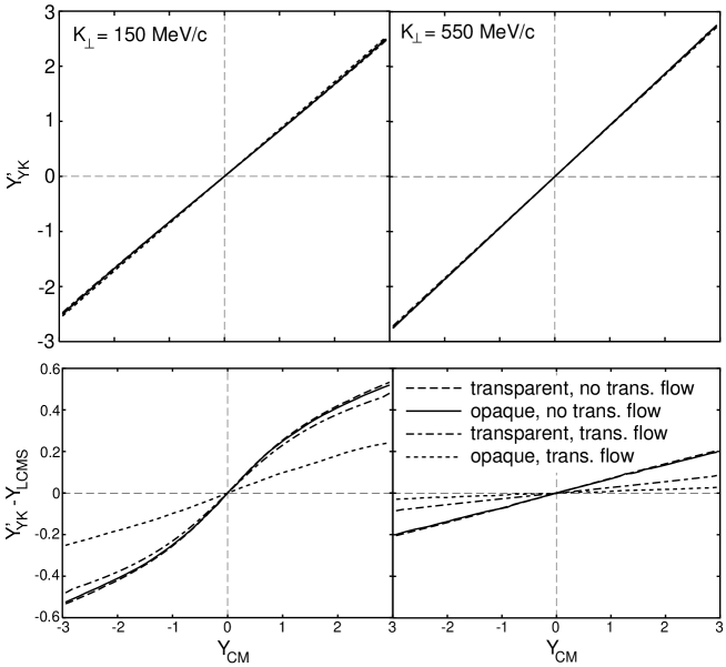
Figure 10: The modified YK rapidity $Y_{{}_{\rm YK}}^{\prime}$ in the CMS (upper row) as a function of the pion pair rapidity in the CMS, for two values of $K_{\perp}=150\,\mbox{\rm MeV/}c$ (left) and 550 MeV/$c$ (right). Line symbols and model parameters as in Fig. 9.

The difference between $Y^{\prime}_{{}_{\rm YK}}$ and the longitudinal flow rapidity $Y_{{}_{\rm LSPS}}$ around the point of maximum emissivity (see lower row of Fig. 10) is somewhat larger than for the original YK rapidity for transparent sources [10, 7], but still small enough to consider $Y^{\prime}_{{}_{\rm YK}}$ as a good approximation for the rapidity of the effective source. The difference between $Y^{\prime}_{{}_{\rm YK}}$ and the rapidities of the LCMS and LSPS disappears in the limit $K_{\perp}\to\infty$, as for the original YK rapidity. Opacity effects on $Y^{\prime}_{{}_{\rm YK}}$ are seen to be small.

5 Conclusions

The most important result found here is that a significant opaqueness of the source leads to dramatic effects on the YKP radius parameter $R_{0}^{2}$. Opaqueness was parametrized by the opacity, i.e. the ratio between the Gaussian transverse geometric radius $R$ and the surface thickness or mean free path, $\omega=R/\lambda$. Even for moderate values of $\omega$, $\omega\sim 1$, $R_{0}^{2}$ becomes negative at small, but experimentally easily accessible values of $K_{\perp}$. For higher opacities this feature extends over larger $M_{\perp}$ regions. For $\omega>1$ the effect should be clearly visible in the existing data from Pb+Pb collisions at CERN.

However, we also encountered a problem which made the comparison with data slightly problematic: we discovered previously unknown regions of inapplicability of the YKP parametrization of the correlation function. These regions of inapplicability are connected with the use of $q_{\perp}=\sqrt{q_{s}^{2}+q_{o}^{2}}$ instead of $q_{s}$ as an independent relative momentum variable. We found that for opaque sources the YK velocity may become ill-defined. For this situation we suggested a modified YKP parametrization which is always well-defined and particularly suited for opaque sources. Even for transparent sources it can always be used as a technical tool to check the correct convergence of the YKP fit, by using the relations (29)-(31). On the physical level, the modified YK velocity $v^{\prime}$ can again be interpreted, in good approximation, as the longitudinal velocity of the effective source. It continues to reflect the longitudinal expansion of the source through a strong dependence on the rapidity of the emitted pairs. The interpretation of the modified transverse and longitudinal radius parameters $R^{\prime}_{\perp}$ and $R^{\prime}_{\parallel}$ as transverse and longitudinal regions of homogeneity in the source rest frame remains valid with sufficient approximation. The interpretation of $R_{0}^{\prime 2}$ (which is now always positive) as the square of the effective source lifetime, however, is spoiled by a large geometric correction. The extraction of a reliable estimate of the source lifetime for opaque sources thus appears to be a very difficult problem.

From the fact that the published data [11] show only positive values for $R_{0}^{2}$ we concluded that the experiment favors a source with volume-dominated emission. Pion freeze-out in heavy-ion collisions thus appears to be similar to the decoupling of the microwave background radiation in the Early Universe: at a certain point in time, when the matter has become sufficiently dilute and cool, suddenly the entire fireball (universe) becomes transparent. However, since for large opacities and in the rapidity region covered by the published data [11] the YKP parametrization was found to break down in the critical region of negative $R_{0}^{2}$, two additional checks are required to confirm this conclusion: the $M_{\perp}$-dependence of the YKP radii at midrapidity should be published, and a careful cross-check of the fitted correlation radii with the Cartesian and/or modified YKP parametrizations should be performed, using the relations given in Sec. 4 and in [7, 10]. In addition to boosting our confidence in the correct convergence of the multidimensional fit to the measured correlation function, such a cross-check would also exclude possible doubts about the applicability of the YKP parametrization to the data. Without doing that one can still try to draw conclusions based on the difference $R_{o}^{2}-R_{s}^{2}$ at small $K_{\perp}$, but compared to the opacity signal carried by $R_{0}^{2}$ this difference is expected to be smaller and more difficult to measure accurately.

Acknowledgments: We are indebted to Harry Appelshäuser, Daniel Ferenc, Henning Heiselberg, Axel Vischer, and Urs Wiedemann for stimulating and clarifying discussions. U.H. thanks the Institute for Nuclear Theory in Seattle for its hospitality and for providing a stimulating environment while this paper was completed. Financial support by DAAD, DFG, BMBF, and GSI is gratefully acknowledged.

Appendix A Definition range for the YKP parameters

The Yano-Koonin velocity $v$ in (8) is only defined if the discriminant

$$D=(A+B)^{2}-4C^{2}$$ (36)

is positive. Here we study the conditions under which this is the case. To this end we write the expressions (12)-(14) as

$$A = A^{\prime}-\frac{1}{\beta^{2}_{\perp}}\langle\tilde{y}^{2}\rangle\,,$$ (37)

$$B = B^{\prime}-\frac{\beta^{2}_{l}}{\beta^{2}_{\perp}}\langle\tilde{y}^{2}\rangle\,,$$ (38)

$$C = C^{\prime}-\frac{\beta_{l}}{\beta^{2}_{\perp}}\langle\tilde{y}^{2}\rangle\,.$$ (39)

We then have

$$A^{\prime} = \left\langle\left(\tilde{t}-\frac{1}{\beta_{\perp}}\tilde{x}\right)^{2}\right\rangle\geq 0$$ (40)

$$B^{\prime} = \left\langle\left(\tilde{z}-\frac{\beta_{l}}{\beta_{\perp}}\tilde{x}\right)^{2}\right\rangle\geq 0$$ (41)

$$C^{\prime} = \left\langle\left(\tilde{t}-\frac{1}{\beta_{\perp}}\tilde{x}\right)\left(\tilde{z}-\frac{\beta_{l}}{\beta_{\perp}}\tilde{x}\right)\right\rangle$$ (42)

and thus

$$|A^{\prime}+B^{\prime}|=A^{\prime}+B^{\prime}\,.$$ (43)

We will prove that

$$(A^{\prime}+B^{\prime})^{2}-4{C^{\prime}}^{2}\geq 0$$ (44)

or

$$|A^{\prime}+B^{\prime}|-2|C^{\prime}|\geq 0\,.$$ (45)

Due to (43) the inequality (45) can be written as

$$A^{\prime}+B^{\prime}\mp 2C^{\prime}\geq 0$$ (46)

where the upper sign stands for $C^{\prime}>0$ and the lower for $C^{\prime}<0$. Inserting expressions (40)-(42) we obtain

$$A^{\prime}+B^{\prime}\mp 2C^{\prime}=\left\langle{\left\{\left(\tilde{t}-\frac{1}{\beta_{\perp}}\tilde{x}\right)\mp\left(\tilde{z}-\frac{\beta_{l}}{\beta_{\perp}}\tilde{x}\right)\right\}}^{2}\right\rangle\geq 0\,.$$ (47)

This proves (44). Since $A^{\prime}$, $B^{\prime}$, and $C^{\prime}$ are the shorthands belonging to the modified YKP parametrization, we have also proven that this parametrization is defined everywhere (except, of course, the point $K_{\perp}=\beta_{\perp}=0$ [7, 10]).

From expressions (37)-(39) we see that

$$A+B = A^{\prime}+B^{\prime}-\frac{1+\beta_{l}^{2}}{\beta_{\perp}^{2}}\langle\tilde{y}^{2}\rangle$$ (48)

$$2C = 2C^{\prime}-\frac{2\beta_{l}}{\beta_{\perp}^{2}}\langle\tilde{y}^{2}\rangle\,.$$ (49)

It is therefore possible to obtain negative values for $D$:

$$D=(A+B)^{2}-4C^{2}<0\,.$$ (50)

For example, if $\beta_{l}=0$ and $\langle\tilde{y}^{2}\rangle$ is fixed at a value bigger than $\langle\tilde{x}^{2}\rangle$, one can find values for $\beta_{\perp}$ such that

$$|A+B|=\left|A^{\prime}+B^{\prime}-\frac{1}{\beta_{\perp}^{2}}\langle\tilde{y}^{2}\rangle\right|<2|C^{\prime}|=2|C|\,.$$ (51)

We must therefore conclude that there are kinematical regions where the YKP parametrization is not defined.

References

- [1] B. Tomášik and U. Heinz, Eur. Phys. Jour. C, in press (Los Alamos e-print archive nucl-th/9707001).
- [2] H. Heiselberg and A.P. Vischer, Eur. Phys. J. C 1 (1998) 593.
- [3] H. Heiselberg and A.P. Vischer, Los Alamos e-print archive nucl-th/9703030.
- [4] B. Schlei and U. Heinz, unpublished.
- [5] T. Csörgő and B. Lörstad, Phys. Rev. C 54 (1996) 1390.
- [6] S. Chapman, J.R. Nix, and U. Heinz, Phys. Rev. C 52 (1995) 2694.
- [7] Y.-F. Wu, U. Heinz, B. Tomášik, and U.A. Wiedemann, Eur. Phys. J. C 1 (1998) 599.
- [8] S. Chapman, P. Scotto, and U. Heinz, Phys. Rev. Lett. 74 (1995) 4400.
- [9] U.A. Wiedemann, P. Scotto and U. Heinz, Phys. Rev. C 53 (1996) 918.
- [10] U. Heinz, B. Tomášik, U.A. Wiedemann, and Y.-F. Wu, Phys. Lett. B 382 (1996) 181.
- [11] H. Appelshäuser et al. (NA49 collaboration), Eur. Phys. J. C, in press (Los Alamos e-print archive hep-ex/9711024).
- [12] G. Roland et al. (NA49 collaboration), proceedings of Quark Matter ’97, December 1.-5., 1997, Tsukuba, Japan, Nucl. Phys. A, in press.
- [13] U.A. Wiedemann and U. Heinz, Phys. Rev. C 56 (1997) 610 and 3265.
- [14] M. Herrmann and G.F. Bertsch, Phys. Rev. C 51 (1995), 328.
- [15] S. Chapman, P. Scotto, and U. Heinz, Heavy Ion Physics 1 (1995) 1.
- [16] K.S. Lee, U. Heinz, and E. Schnedermann, Z. Phys. C 48 (1990) 525; E. Schnedermann, J. Sollfrank, and U. Heinz, Phys. Rev. C 48 (1993) 2462.
- [17] T. Csörgő and B. Lörstad, Nucl. Phys. A 590 (1995) 465c.
- [18] P. Jones et al. (NA49 Collaboration), Nucl. Phys. A 610 (1996) 188c.
- [19] S. Schönfelder, PhD thesis, MPI für Physik, München (1996), NA49 Note 143, available at URL http://na49info.cern.ch.
- [20] U. Heinz, in Hirschegg ’97: QCD Phase Transitions, H. Feldmeier et al., eds., GSI Report, 1997 (Los Alamos e-print archive nucl-th/9701054); U. Heinz, Los Alamos e-print archive nucl-th/9710065, to appear in the Proceedings from the 5th Rio de Janeiro International Workshop on Relativistic Aspects of Nuclear Physics, Aug. 1997, (T. Kodama, ed.), World Scientific, Singapore, 1998.
- [21] U.A. Wiedemann, B. Tomášik, and U. Heinz, proceedings of Quark Matter ’97, December 1.-5., 1997, Tsukuba, Japan, Nucl. Phys. A, in press (Los Alamos e-print archive nucl-th/9801017).
- [22] B. Kämpfer, Los Alamos e-print archive hep-ph/9612336.
- [23] B.R. Schlei and N. Xu, Phys. Rev. C 54 (1996) R2155.
- [24] A.N. Makhlin and Y.M. Sinyukov, Z. Phys. C 39 (1988) 69.
- [25] H. Appelshäuser, PhD. thesis, J.W. Goethe–Universität Frankfurt am Main (1996), NA49 Note 150, available at URL http://na49info.cern.ch.
- [26] A. Sakaguchi et al. (NA44 Collaboration), talk presented at Quark Matter ’97, December 1.-5., 1997, Tsukuba, Japan, Nucl. Phys. A, in press.
- [27] K. Kadija et al. (NA49 Collaboration), Nucl. Phys. A 610 (1996) 248c.
- [28] B. Lasiuk, Acta Phys. Slovaca 47 (1997) 15.