A model for nuclear matter fragmentation: phase diagram and cluster distributions

Abstract

We develop a model in the framework of nuclear fragmentation at thermodynamic equilibrium which can be mapped onto an Ising model with constant magnetization. We work out the thermodynamic properties of the model as well as the properties of the fragment size distributions. We show that two types of phase transitions can be found for high density systems. They merge into a unique transition at low density. An analysis of the critical exponents which characterize observables for different densities in the thermodynamic limit shows that these transitions look like continuous second order transitions.

PACS: 25.70.Pq, 64.60.Cn, 64.60.Fr.

Key words: Nuclear fragmentation. Phase transitions. Monte Carlo. Ising model. Kawasaki dynamics.

1 Introduction

The fragmentation of excited nuclei is a complex, time-dependent process. There exists however experimental evidence if no proof that the decaying system can be treated as a thermodynamically equilibrated assembly of interacting particles, at least in specific experimental circumstances [1]. If this is the case, the fragmentation process evolves in time by following trajectories in the $(\rho,T)$ phase diagram ($\rho$ is the density and $T$ the temperature). It starts at some initial point and ends at a final point when the freeze-out stage is reached. During the time interval in which this goes on, the initial excited system breaks into fragments and (or) evaporates particles.

As far as such a scenario corresponds to a physical realization of the process, one is left with two types of experimentally relevant physical observables. The first set concerns the thermodynamic properties of the expanding system (energy, temperature, pressure and correlations between these quantities, possible existence of phase transitions). The second set concerns final fragment size distributions and related observables.

The latter observables have been rather extensively studied in numerous experiments, showing remarkable properties [2] which were analyzed by means of different types of models. These analyses lead to the conclusion that the system may undergo a second order transition which lies in the universality class of bond percolation in three dimensions [3].

The thermodynamic properties of fragmenting nuclei are less well known from the experimental point of view. There are indications for the existence of two phases which could be analogous to liquid and gas in macroscopic systems. The order of the transition between the two phases is not clearly established either [4, 5, 6]. Successful multifragmentation models [7, 8, 9] which are able to reproduce a large amount of experimental data predict a first order transition.

Running parallel to the experimental efforts in order to characterize the behaviour of the system, realistic theoretical models should aim and be able to describe both aspects, the thermodynamic properties as well as the characteristics of the fragment size distributions in a consistent way. This has already been attempted in recent work in the framework of the lattice gas model (LGM) [10, 11, 12, 13] and to some extents by means of homogeneous cellular models [14].

It is the aim of the present paper to present a detailed analysis of both properties by means of a simple though quite realistic model, to identify the phases in which the system can exist and the order of the corresponding phase transitions.

The paper is arranged in the following way. In section 2 we describe the model. We emphasize its kinship with other models and its specific features. In section 3 we first define the observables which we consider in the sequel and work out the phase diagram which links the density to the temperature. We then analyze the properties of the phase transitions which appear in the system in section 4. We summarize, conclude, present and discuss further possible developments in section 5.

2 Spin models and fragmentation

2.1 The lattice gas model and the Ising model

The lattice gas model (LGM) describes the motion of $N=\rho\cdot V$ particles inside a three-dimensional cubic lattice, where $\rho$ is the average density, $0\leq\rho\leq 1$, and $V$ the number of sites. Particles which occupy sites in this volume interact only when they are nearest-neighbours. If $n_{i}=0,1$ are the site occupation numbers (empty/occupied), and $\mu$ is the chemical potential, the Hamiltonian reads

$$H_{V}=-4J\sum_{\langle i,j\rangle\subset V}n_{i}n_{j}+\mu\sum_{j\in V}n_{j},$$ (1)

where $\langle ij\rangle$ are nearest neighbour cells.

The formulation presented in eq. (1) corresponds to the grand canonical ensemble. The microcanonical ensemble is the most natural ensemble to be used when describing nuclear fragmentation since nuclei are closed systems with fixed energy and number of particles. It is usually assumed that the thermodynamic results are the same independently of the formalism used. Of course this is not true with finite systems, because microcanonical, canonical and grand canonical ensembles differ on the level of fluctuations. But it has recently been argued [15] that even in the thermodynamic limit, microcanonical and (grand)canonical ensembles are not equivalent (for example, at a first order transition). We shall explicitely show in this paper that in fact the canonical and grand canonical formulations of the LGM are not equivalent. This happens because there are points in the phase diagram which are accessible when using one formalism, but are not defined (they are not points of thermodynamic equilibrium) when using another one. As we will see, this causes the order of the transition to be different in the two formalisms. This fact leads us naturally to ask about the behaviour of the system in the microcanonical ensemble. This is an open problem, but as a first step we will consider here only the detailed study of the canonical formulation to compare it with the well-known grand canonical version of this model. In fact, for sytems with finite volume, the microcanonical ensemble turns out to be very efficient in the study of phase transitions [16, 17].

This simple model can be numerically studied, its grand partition function being proportional to the canonical partition function of the Ising model with an external magnetic field [18]. In fact, setting

$$\sigma_{j}=2n_{j}-1,$$ (2)

the Hamiltonian (1) becomes

$$H_{V} = -J\sum_{\langle i,j\rangle\subset V}\sigma_{i}\sigma_{j}+\left(\frac{\mu}{2}-6J\right)\sum_{j\in V}\sigma_{j}+\mathrm{const}(V)$$

$$\equiv -J\sum_{\langle i,j\rangle\subset V}\sigma_{i}\sigma_{j}-h\sum_{j\in V}\sigma_{j}+\mathrm{const}(V),$$

where we reinterpret $\sigma_{j}=\pm 1$ as a spin variable, and identify a spin up with an occupied site, and a spin down with an empty site. We introduce

$$M\equiv\frac{1}{V}\sum_{j}\sigma_{j}=\frac{1}{V}(2N-V)=2\rho-1.$$ (4)

$M$ is called the magnetization in the sequel. As it can be seen, the initial model defined through (1) can indeed be mapped on an Ising model with a linear term corresponding to a fixed magnetic field $h$.

It is well known that the Ising model with magnetic field $h$ presents a discontinuity in the magnetization $M(h,T)$ for $T<T_{c}$ at $h=0$, where $T_{c}$ is the critical temperature. That is, in the plane $(h,T)$ there exists a line of first-order transitions $(h=0,\,0\leq T<T_{c})$, and a second order transition at $(h=0,T_{c})$. Let us see how this is reflected in the case of the LGM. Since $h$ plays essentially the role of the chemical potential in the grand canonical formulation of the LGM, there is a first order transition in the phase diagram $(\rho,T)$ of the LGM, which separates the homogeneous phase from the zone with the two “liquid” and “gas” phases. On this line, there exists a critical point at $\rho=0.5$, $T=T_{c}$.

As described below, we aim to introduce a similar type of model in order to describe a finite, excited system of classical particles which interact by means of a short range potential. We characterize the internal structure of the system by means of a proper definition of physical droplets. Droplets are clusters of particles in which each particle has at least one nearest neighbour. They exist because of two physical reasons: the attractive nearest-neighbour interaction and the density of particles, which leads to usual percolation when this density is large enough. However, such clusters are not always stable, because they can break at zones of small connectivity owing to the kinetic energy of the particles. The simple model (equivalently, the LGM) does not take the kinetic energy into account. We can introduce this energy by means of another definition which takes the energetics of the fragmentation into account [10, 11]. Let us consider the stability of a cluster of $A$ particles. If the loss of a particle implies the break of a single bond, then the excess of energy will be

$$\frac{-p^{2}}{2m}+J,$$ (5)

where $m$ is the mass of the particles of the LGM. The cluster is a stable droplet if this excess is positive:

$$\frac{p^{2}}{2m}-J<0.$$ (6)

This suggests to introduce a bond probability $p^{\prime}_{b}\leq 1$ for the nearest neighbour particles to belong to the same droplet:

$$p^{\prime}_{b}=\mathrm{Prob}\left(\frac{p^{2}}{2m}-J<0\right),$$ (7)

where $p$ is distributed according to a Maxwell law, that is, the probability for a particle to have a momentum $p$ is

$$\mathrm{Prob}(\mbox{\boldmath$p$})=\frac{1}{[2\pi k_{\mathrm{B}}T]^{3/2}}\,\exp\left(\frac{\mbox{\boldmath$p$}}{2mk_{\mathrm{B}}T}\right).$$ (8)

One can see that the choice of the bond probability (7) allows to extend the argument to the case in which the loss of a particle of the cluster means the break of several bonds [10]. We obtain:

$$p^{\prime}_{b} = \mathrm{Prob}\left(p^{2}<2mJ\right)=1-\mathrm{Prob}\left(p^{2}>2mJ\right)$$ (9)

$$= 1-\frac{4\pi}{[2\pi mk_{\mathrm{B}}T]^{3/2}}\int_{\sqrt{2mJ}}^{\infty}e^{-p^{2}/2mk_{\mathrm{B}}T}p^{2}\,\mathrm{d}p$$

$$= 1-\frac{4}{\sqrt{\pi}}\int_{\sqrt{J/k_{\mathrm{B}}T}}^{\infty}u^{2}e^{-u^{2}}\,\mathrm{d}u.$$

Performing a Laguerre expansion, one finds [10]

$$p^{\prime}_{b}=1-0.911e^{-J/2k_{\mathrm{B}}T}-0.177\left(1-\frac{J}{k_{\mathrm{B}}T}\right)e^{-J}{2k_{\mathrm{B}}T}+\cdots$$ (10)

which shows the similarity between the bond probability definition (7) and the Coniglio-Klein distribution of probability

$$p_{b}=1-e^{-2J/k_{\mathrm{B}}T}.$$ (11)

We will use this much simpler bond probability to simulate the kinetic energy contribution. This definition of bond-correlated percolation has also the advantage that the droplets percolate at the thermodynamic transition point with the exponents of the Ising model [19]. This is not true in general with the site-correlated percolation given by the Ising clusters ($p_{b}=1$).

2.2 Previous results

The LGM has been introduced in order to describe fragmentation. In refs. [11, 12] several analytical simplifications were made on the model, as well as numerical simulations taking the analogy with the Ising model at fixed magnetic field. The authors used a definition of droplets which lead the thermal critical point to coincide with a percolation point. Recently the authors of refs. [11, 12] have also considered isospin-dependent interactions, and they have determined the distribution of clusters together with other observables [13]. Similar studies can be found in ref. [20].

In ref. [10] it was noted that there exists a full line, not only a single point, in the phase diagram of the LGM, for densities larger than 0.5, where distributions of fragment sizes which obey a power law distribution are obtained. On this line, which is very close to the Kertész line [21], one finds a phase transition because the droplets are defined with a physical prescription. Along this transition, there are no discontinuities for any thermodynamic quantities (energy, specific heat,…). However, for some nonlocal quantities, as clusters, a discontinuity appears. The critical exponents along this line (outside of the critical point) should give some clue about the kinship with a percolation transition.

2.3 Present model: Ising with fixed number
of particles

In all the numerical calculations mentioned above, the LGM is equivalent to the Ising model with a constant magnetic field. This corresponds to a fixed chemical potential. Hence the number of particles (and consequently, the density) is conserved on the average in the framework of the grand canonical formalism. For systems as small as nuclei, it is certainly appropriate to consider the model with a fixed number of particles, which corresponds to the canonical ensemble. As it was stated above, the nucleus is a closed system without heat bath. Under these conditions, the microcanonical ensemble is the most appropriate formalism to use, but we will leave the constraint of the energy as an open problem and concentrate on the crucial difference which exists between the canonical and the grand canonical in this case. The reason is that the constraint of fixed number of particles can not always be satisfied with the last formalism, in sharp contrast with the situation in the former framework as we shall see.

The LGM in the canonical formalism is just the Ising model with fixed magnetization (IMFM), here with fixed number of particles. We introduce the following partition function

$$\mathcal{Z}_{V}=\sum_{[\sigma]}e^{\beta\sum_{\langle ij\rangle}\sigma_{i}\sigma_{j}}\,\cdot\delta(M-\hat{M}),$$ (12)

where $\beta=J/k_{\mathrm{B}}T$ (we take $J/k_{\mathrm{B}}=1$ for simplicity), $\hat{M}\in[-1,1]$ is a fixed number, and the delta function constrains the configurations $[\sigma]$ which contribute to the sum to those with fixed density, so that $M=\hat{M}$, where $M$ is defined in (4) above.

As already stated above, the grand canonical formalism of the LGM is the Ising model with constant $h$. Of course an Ising model with a magnetic field $h$ which produces a magnetization $\langle M\rangle$ at a certain value of $\beta$ is equivalent in the thermodynamic limit (that is, it gives the same value for the different observables) to the model (12) with magnetization $\hat{M}=\langle M\rangle$ and the same $\beta$. This is so because in the limit $V\to\infty$, the fluctuations in $M$ are negligible, and the distribution is a Dirac delta centered in $\langle M\rangle$.

But, reversely, the description of a model with fixed magnetization is not necessarily equivalent to a model with fixed magnetic field in the grand canonical ensemble: in the LGM (we will refer from now on to the LGM as the model considered in the grand canonical formalism), we obtain a certain mean magnetization (or density, see eq. (4)) with a magnetic field $h$ at some value of $\beta$. When we increase $\beta$, we have to lower $h$ in order to get the same value of $\langle M\rangle$. It is always possible to find a value of $h$ which gives a fixed $\langle M\rangle$ while $\beta<\beta_{c}(h=0)$. However, for $\beta>\beta_{c}$, there is an spontaneous magnetization $\langle M(\beta)\rangle$, and the presence of a magnetic field $h\neq 0$ can only increase $|\langle M(\beta)\rangle|$, therefore values of $|\langle M\rangle|<|\langle M(\beta)\rangle|$, are not accessible in the grand canonical formalism. In fact, these non-equilibrium states are separated from the normal states by the first order transition in $\beta$ mentioned in section 2.1.

However, we can still consider the values of $\beta$ and the magnetization that correspond to non-equilibrium states in the LGM, in the framework of the model (12). They will correspond to a definite mean value of the energy, for example. These points of the phase diagram are points of thermodynamic equilibrium of the model (12). Hence one may ask about the behaviour of the energy when crossing the corresponding transition point of the LGM and the existence of a phase transition at this point in the present model. We aim to investigate this point in the sequel, as well as its consequence on the behaviour of the fragment size distributions.

2.4 Update algorithm

The Ising model with constant order parameter (magnetization $M$) has been considered previously from the point of view of its critical dynamic exponents (see, eg [22]), but it seems that its equilibrium properties have not been addressed [23]. The corresponding dynamics would be in principle that of the Kawasaki spin exchange model [24], but, as the authors of [23] noted, one should take special care with the detailed balance in a numerical algorithm for this model.

In our Monte Carlo computations, the following update algorithm has been used: two spins are picked up at random, and they are exchanged according to the standard Metropolis prescription [25] only if they have different signs. This algorithm preserves the magnetization (that is, the number of spins up, which represent the particles), and it can easily be seen that it satisfies detailed balance.

In fact it is striking to notice how one can arrive to non-Boltzmann distributions if one does not care very much about the update procedure. For example, we also considered the following algorithm: take one spin sequentially on the lattice and another one at random, and exchange them only if they have different signs. This does not satisfy detailed balance, as the following argument shows. Consider an initial configuration with every spin up except for a single spin down. Suppose that the sequential process is such that we have to take the spin at the position $i=0$, which is up. With the algorithm described, there is only a possible final configuration, the one in which the spin down has been exchanged with the spin up at $i=0$. If we consider now the reverse process, we have to exchange the spin down at $i=0$ with a spin up. But now we have many final configurations, not only the initial one, so it is clear that this process does not satisfy detailed balance. We can modify this sequential algorithm to solve the problem. If the spins taken sequentially and randomly are always exchanged, independently of their sign, detailed balance is restored. We verified this numerically, so that the results with this last algorithm were the same as with the ‘full randomly’ algorithm described above. In fact, an interesting property of this ‘random’ algorithm in which the two spins are taken at random is that here one can choose exchanging the spins in every case, or only when having different signs. Both situations verify detailed balance, as we checked numerically, thanks to the randomness in the choice of the spins.

Similar subtleties happen in algorithms where nearest neighbours are exchanged, as in Kawasaki dynamics, which were first noted in [23].

3 The $(\rho,T)$ phase diagram and
cluster formation

3.1 Definition of observables

We simulate the IMFM, defined by eq. (12), in a three-dimensional cube of $V=L^{3}$ sites, and with $N=\rho\cdot V$ spins up and periodic boundary conditions. We work out the phase diagram in the $(\rho,\beta)$ plane.

The thermodynamic observables are the energy

$$E=\frac{1}{3V}\sum_{\langle i,j\rangle}\sigma_{i}\sigma_{j},$$ (13)

and its $\beta$ derivative, the specific heat

$$C_{v}=3V\cdot\left(\langle E^{2}\rangle-\langle E\rangle^{2}\right).$$ (14)

The droplet observable which we consider is the second momentum

$$S_{2}=\sum_{s}s^{2}P(s),$$ (15)

where $P(s)$ is the number of droplets of size $s$, and the sum extends over all droplets except for the largest one.

The droplets are defined from the Ising clusters with the probability law (11). With this definition, the transition properties of the thermodynamic transition, given by the divergence of $C_{v}$, and the droplet transition, given by the divergence of $S_{2}$, coincide in the standard Ising model (constant magnetic field) at $h=0$. We want to see whether this is also the case in the IMFM.

3.2 Phase diagram and cluster formation

The phase diagram of the IMFM should be the same as the one of the LGM because the thermodynamic relations between the different quantities must be the same in the domain where the LGM displays an homogeneous phase. The thermodynamic transition lines must coincide in both phase diagrams. However, the nature of this transition can be different, as noticed above.

Figure 1: Plot of $M(T)$ in the Ising model at $h=0$ magnetic field, and trajectory of constant magnetization.

We can also understand physically the existence of a phase transition in the Ising model with constant magnetization with the help of Fig. 1. It shows the curve $M(T)$ for the usual Ising model at $h=0$ magnetic field. Constraining the system to move in $T$ with fixed magnetization $\hat{M}$ (indicated by the dashed line) will be equivalent to pass through Ising models with different values of $h$ (those which give the magnetization $M(T)=\hat{M}$ at each $T$), until one finally reaches the $M(T)$ curve corresponding to $h=0$. Then it is not possible to go to the left in the usual Ising model with any magnetic field, but this is possible with the present model. One expects a phase transition at that point, and this will be confirmed below. Therefore, the curve $M(T)$ plotted in Fig. 1 will exactly correspond to the transition line of this model in the $(\rho,\beta)$ plane.

In Fig. 2 we plot the phase diagram obtained directly in a numerical simulation of an $L=20$ lattice. We represent the thermodynamic transition (maximum of the specific heat, divergence in the infinite volume limit) and the droplet transition (maximum of $S_{2}$). For $L=20$ these transitions are different, but a priori this could be a finite size effect. We shall see in the next sections whether these two transitions are the same. The thermodynamic transition is symmetric with respect to $\rho=0.5$, because the thermodynamic properties are the same in terms of spins up or down, that is, the model has a symmetry $\sigma\leftrightarrow-\sigma$ which corresponds to $\rho\leftrightarrow 1-\rho$. The droplet transition is not symmetric because we define only droplets for sites corresponding to $\sigma=+1$. In Fig. 2 the thermodynamic transition for $L=20$ presents an “anomaly” at $\rho=0.5$ so that the curve seems not to be concave there. This is a finite size effect, due to the fact that the critical exponents vary along the line, as we will see in section 4. Then the thermodynamic limit is reached differently at different points on the line. Actually, we have included in the Figure the infinite volume curve obtained from the values of the critical points at $\rho=0.3$ and $\rho=0.5$ calculated in section 4.3.

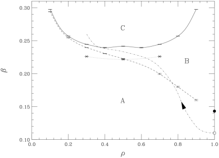
Figure 2: Phase diagram of the Ising model with constant magnetization, obtained numerically from an $L=20$ $3d$ cubic lattice. The solid line is the thermodynamic transition and the dashed line the droplet transition. The dotted line indicates the infinite volume limit of the thermodynamic transition (see text). The black point at $\rho=1$ is the three-dimensional bond-percolation point. The line with the arrow (dot-dashed) symbolizes a typical trajectory, see text.

The region A in Fig. 2 is the disordered region, B is a region where an infinite cluster is formed but the spin system, from a thermodynamic point of view, is disordered, and C is a region with an infinite cluster which also corresponds to an ordered thermodynamic system. The thermodynamic transition is the line which separates the regions B and C, and the droplet transition is the one which separates the regions A and B.

The physical origin of the infinite cluster is, on the one hand, the Ising-type interaction, which, in the nuclear context, simulates the strong interaction between the particles. The most probable configuration for large $\beta$ is that with all spins up together, forming a spherical cluster. This is only relevant in region C. On the other hand, the density also influences the development of clusters, because we know that, even in absence of interaction, the system percolates when there are many particles. This effect appears in region B, and this is the reason why the droplet transition separates from the thermodynamic one for large values of $\rho$. Besides that, $\beta$ also influences the formation of physical droplets through the bond probability (11), simulating a kinetic energy for the particles depending on the temperature: the lower the temperature, the less the particles can move.

Far inside the ordered phase, the system favours the configuration which minimizes the energy, and then a large cluster is formed. All occupied sites inside the cluster contribute positively to the energy, as well as those outside the cluster ($\sigma_{i}\sigma_{j}=+1$). The only contributions with $\sigma_{i}\sigma_{j}=-1$ are those located at the border, so that the configuration will show a minimal surface, something very similar to a sphere. One can estimate the energy in this case. Let us consider a cubic shape for this cluster. Then, the total amount of (potential) energy is

$$E_{T}=3V\left(1-\frac{4\rho^{2/3}}{V^{1/3}}\right),$$ (16)

so that

$$E=\frac{E_{T}}{3V}=1-\frac{4\rho^{2/3}}{L},$$ (17)

and in the thermodynamic limit $(L\to\infty)$, $E$ is normalized to 1. This is why we chose the factor $3V$ in the normalization of $E$ and $C_{v}$ in eqs. (13) and (14).

3.3 Cluster distribution and nuclear fragmentation

Along the droplet transition, the observable $S_{2}$ diverges, because there the fragment size distribution $P(s)$ follows a power law

$$P(s)\sim s^{-\tau}.$$ (18)

A possible fragmentation scenario can be suggested in the $(\rho,\beta)$ diagram of Fig. 2 (dot-dashed line). Consider a nuclear collision leading to an excited system of $N$ particles in a volume $V$, in thermodynamic equilibrium or at least close to it. This point would correspond to a rather large density ($\rho\approx 1$) and small $\beta$ (large temperature), lying below the droplet transition line. The trajectory would then move towards decreasing $\rho$ and increasing $\beta$. It would cross the critical droplet line at some point $(\rho_{0},\beta_{0})$ and pursue its way towards lower density and temperature, up to some freeze-out where the fragment size distribution gets fixed. From thereon the system would continue to cool down and expand continuously, crossing the thermodynamic transition line at some other point. In practice, of course, the system follows a whole set of trajectories corresponding to different experimental initial conditions (system, energy, impact parameter,…). Unfortunately it is not possible to get direct information about these trajectories. There could exist indications that the crossing of the critical droplet line may occur for rather high values of the density. In fact, indirect experimental information (agreement with percolation results) indicates that the exponent $\tau$ could lie close to the value 2.2 which corresponds to $\rho>0.5$ (see section 4.4 below). On the other hand, molecular dynamics (MD) calculations seem to indicate that the system breaks up rather early during the collision process [26]. Whether the critical $\tau$ can be put in direct correspondence with experimental measurements of fragment distributions which correspond to averages over different events remains however an unsettled question.

4 Phase transitions and their characteristics

4.1 Critical exponents

As we have seen, the phase diagram of the IMFM shows, in principle, two phase transitions. We may ask whether these two transitions coincide for small values of $\rho$, the type of thermodynamic transition and what is its order, its universality class, and the value of the exponent $\tau$, whether it is constant or not along the transition line.

The critical exponents will bring an answer to these questions. We have two observables which diverge at their corresponding transitions in the thermodynamic limit, the specific heat

$$C_{v}\sim(\beta-\beta_{c}^{\mathrm{T}})^{-\alpha},$$ (19)

which defines the exponent $\alpha$, and the second momentum

$$S_{2}\sim(\beta-\beta_{c}^{\mathrm{D}})^{-\bar{\gamma}},$$ (20)

which defines the exponent $\bar{\gamma}$, $\beta_{c}^{\mathrm{T}}$ and $\beta_{c}^{\mathrm{D}}$ correspond to the thermodynamic and droplet transition respectively. Note that in principle, the exponents of the thermodynamic and droplet transitions will be independent, because we have two different models: Ising (with fixed magnetization), and a bond-percolation correlated model, constructed on the IMFM system. We know that in the case of the standard Ising model, the definition (11) of the bond probability is such that the thermodynamic and the droplet exponents are the same, and the position of the transitions coincide. But this could be different in the present case. Actually, the exponent $\gamma$, defined as the one which gives the divergence of the magnetic susceptibility, is not defined for the IMFM, because we keep the magnetization fixed as an external parameter. This is also the case of the remaining “magnetic” exponents, $\beta$ and $\eta$. Therefore, the universality class of the IMFM will be completely determined by $\alpha$ and $\nu$, which should obey the hyperscaling relation

$$\alpha=2-\nu d.$$ (21)

We will denote the exponents corresponding to the droplet transition with a little bar above the corresponding greek letter.

We can measure critical exponents from standard finite size scaling [27, 28]. For finite lattice size $L$, $C_{v}$ and $S_{2}$ show peaks (at different points, $\beta_{c}^{\mathrm{T}}(L)$ and $\beta_{c}^{\mathrm{D}}(L)$, respectively), which scale with $L$ as

$$C_{v}(L) = A+BL^{\alpha/\nu},$$ (22)

$$S_{2}(L) = \bar{A}L^{\bar{\gamma}/\bar{\nu}}.$$ (23)

The exponent $\nu$ can also be obtained from a fit to the law

$$\beta_{c}(L)-\beta_{c}(\infty)=AL^{-1/\nu},$$ (24)

where $\beta_{c}(\infty)$ is the thermodynamic value of the transition point, and $\beta_{c}(L)$ is the value of $\beta$ where the thermodynamically divergent observable has a maximum at finite $L$.

The exponents of the droplet transition will also obey the corresponding scaling and hyperscaling relations

$$\frac{\bar{\gamma}}{\bar{\nu}} = 2-\bar{\eta},$$ (25)

$$\bar{\alpha}+2\bar{\beta}+\bar{\gamma} = 2,$$ (26)

$$\bar{\alpha} = 2-\bar{\nu}d,$$ (27)

where these exponents are defined by the behaviour of various moments of the cluster size distributions, see eg [29].

Using scaling and hyperscaling with $d=3$, the exponent $\tau$ of the distribution of fragments can be obtained directly from $\bar{\eta}$:

$$\tau=2+\frac{\bar{\beta}}{\bar{\beta}+\bar{\gamma}}=2+\frac{1+\bar{\eta}}{5-\bar{\eta}}=2.2+\frac{6}{25}\bar{\eta}+\mathrm{o}(\bar{\eta}^{2}),$$ (28)

so that if $\bar{\eta}$ is small (which is usually the case), $\tau$ is $2.2$ modified by a small amount. We remark that for all the models with small $\bar{\eta}$ (and for all the standard models in three dimensions, $\bar{\eta}\leq 0.1$), $\tau$ can only vary between 2.1 and 2.3. The only nontrivial result is the deviation from 2.2.

We shall be able to check the validity of these relations through the determination of $\tau$ by means of two independent methods, directly, by measuring the droplet distribution followed by a fit to eq. (18), and by computing the critical exponents with the use of eq. (28).

4.2 The numerical simulation

In order to compute the critical exponents, and to see if the droplet and thermodynamic transitions coincide in the infinite volume limit, we have studied the transitions with large statistics at three different values of $\rho$ in the phase diagram, $\rho=0.3,0.5,0.7$. The peak in $C_{v}$ (eq. (22)) can be easily located with the spectral density method [30], but unfortunately, this is not possible with $S_{2}$, because we construct this observable with bond probabilities for each configuration. This means that the value of $S_{2}$ is not completely determined by the configuration, and then it is not possible to use the spectral density method to extrapolate to different values of $\beta$. Therefore, we have obtained the maximum of $S_{2}$ with less precision than in the case of $C_{v}$.

We studied the thermodynamic transition at $\rho=0.3$ and $\rho=0.5$ (because of the symmetry of this transition, $\rho=0.7$ is equivalent to $\rho=0.3$), in order to fix the exponents $\alpha$ and $\nu$, which inform us about the universality class of the IMFM model. In Table 1 we show the lattice sizes and statistics used, together with the integrated autocorrelation time [31] for the energy.

For the droplet transition we only studied lattices up to $L=24$, first because of the difficulty of finding the peak of $S_{2}$ as mentioned above, and second because the exponent $\tau$ may be a meaningful physical quantity in the case of a finite system, which may eventually be directly or indirectly confronted with the experiment.

In the simulation we proceed as follows: we make 10-15 update steps (in each step the algorithm described in section 2.4 is applied $V$ times), and then we perform a measurement. At this moment the droplets are defined according to (11). Hence we can calculate $S_{2}$. The errors are computed with the jackknife method [32].

	$\rho=0.3$		$\rho=0.5$
$L$	$\tau(E)$	Sweeps $[\times 10^{3}\tau(E)]$	$\tau(E)$	Sweeps $[\times 10^{3}\tau(E)]$
10	8.55(3)	1091	12.15(6)	985
16	12.84(11)	932	22.1(3)	407
20	15.72(12)	381	27.5(3)	345
24	20.84(12)	1061	35.2(2)	680
28	27.2(2)	527	43.7(4)	738
32	33.0(3)	362	53.5(7)	558
40	63.9(1.1)	110	75.3(8)	189
48	109(2)	108	110(7)	43

Table 1: Total number of sweeps or update steps (measurements are performed every 10-15 sweeps) and the corresponding integrated correlation times $\tau$ for $E$, used in the analysis of the thermodynamic transition at $\rho=0.3$ and $\rho=0.5$.

4.3 The thermodynamic transition

We start by considering the nature of the thermodynamic phase transition (solid line in Fig. 2), ie the points in the phase diagram where the specific heat diverges. We show in Fig. 3 the caloric curve ($E$ vs. $\beta$) for two lattice sizes, $L=10,24$. In principle, these kind of curves are not very precise to distinguish the order of the phase transition. A first order transition means a discontinuity in this curve, and a second order one means a vertical slope at the critical line. But this is only true in the thermodynamic limit, $L=\infty$. In a finite lattice there are not singularities at all, and then it is necessary to carry out a careful study of the thermodynamic limit by considering finite size scaling techniques, such as expressions (22) and (23). The values of the critical exponents obtained in this way inform us about the order of the phase transition, and define the universality class in the case of a second order transition. We will show evidences of the second order nature of the transition line at every value of $\rho$. On the one hand, a single peak in the histogram of the energy was observed in all numerical simulations. This is a strong indication of a second order phase transition. On the other hand, this was confirmed by an analysis of the critical exponents $\nu$ and $\alpha$, which show a different behaviour from that of a first order transition ($\alpha=1$, $\nu=1/d=1/3$).

Figure 3: Caloric curve ($E$ vs. $\beta$) for two finite lattice sizes, $L=10$ and $L=24$, at $\rho=0.3$.

Exponents $\nu$ and $\alpha$ determine the universality class of the transition. In order to see the values of these exponents, we have to find the behaviour in the $V\to\infty$ limit. We consider lattice sizes up to $L=48$ and study these exponents by finite size scaling at $\rho=0.3$ and $\rho=0.5$.

In Table 2, we report the values of the thermodynamic transitions and the maxima of $C_{v}$ for the different sizes at $\rho=0.3$ and $\rho=0.5$.

	$\rho=0.3$		$\rho=0.5$
$L$	$\beta_{c}^{\mathrm{T}}$	$C_{v}^{\mathrm{max}}$	$\beta_{c}^{\mathrm{T}}$	$C_{v}^{\mathrm{max}}$
10	0.2698(3)	3.063(5)	0.2778(10)	3.880(7)
16	0.2516(3)	5.109(9)	0.2495(4)	6.380(14)
20	0.2445(2)	6.191(8)	0.2417(2)	7.739(11)
24	0.23988(11)	7.033(7)	0.23694(6)	8.819(9)
28	0.23658(11)	7.758(8)	0.23364(7)	9.726(11)
32	0.23435(11)	8.45(2)	0.23157(8)	10.519(12)
40	0.23152(5)	9.72(2)	0.22862(7)	11.80(3)
48	0.229885(14)	11.11(4)	0.22680(8)	12.93(6)

Table 2: Thermodynamic transition $\beta_{c}^{\mathrm{T}}$ and the maxima of $C_{v}$ for different lattice sizes at $\rho=0.3$ and $\rho=0.5$.

Consider first the case $\rho=0.3$. One needs to make a fit to eq. (22) in order to obtain $\alpha/\nu$. If the constant term is not very important, a plot $\ln C_{v}^{\mathrm{max}}$ vs. $\ln L$ should fit to a straight line of slope $\alpha/\nu$. This plot is shown in Fig. 4, where we see that the slope changes with $L$ for small $L$. This means that corrections to scaling are important. We observe that the slope reaches an asymptotic limit from $L=24$ on. Actually, the fit for $L=24,28,32,40$ is very good:

$$\alpha/\nu=0.634(4)\quad\quad\chi^{2}/\mathrm{DF}=0.290/2,$$ (29)

where DF stands for the number of degrees of freedom in the fit. The $L=48$ point, however, stays a bit away of this value. In fact, if we try to include this point, the fit obtained is not good because we obtain a large $\chi^{2}/\mathrm{DF}$, and it gives a value of $\alpha/\nu=0.643(4)$. It is possible that the failure of this fit is due to a subestimate of the error in this last point, which has a large autocorrelation time (see Table 1). To be cautious, anyway, we will take as the best estimate for $\alpha/\nu$, the value

$$\alpha/\nu=0.639(8).$$ (30)

Figure 4: Plot of $\ln C_{v}^{\mathrm{max}}$ vs. $\ln L$ for $L=10,16,20,24,28,32,40,48$ at $\rho=0.3$ and $\rho=0.5$. A straight line fit should give $\alpha/\nu$. We observe scaling corrections for small $L$ in both cases.

An independent fit from this one is the two-parameter fit to eq. (24), which gives the best fit for $\nu=0.60(4)$. Here the error is very large. Considering instead the result (30), hyperscaling (21) gives for $\nu$ and $\alpha$ the values

$$\nu=0.5496(12)\quad\quad\alpha=0.351(4).$$ (31)

One can check this value of $\nu$ by means of a fit to eq. (24). Taking again the lattices $24\leq L<48$, we obtain

$$\beta_{c}(\infty,\rho=0.3)=0.22606(13)\quad\quad\chi^{2}/\mathrm{DF}=0.881/2,$$ (32)

which is a good fit. If we add the $L=48$ lattice, this value is slightly modified ($\beta_{c}=0.22590(6)$), and the $\chi^{2}/\mathrm{DF}$ is still acceptable (3.5/3). Therefore, we will take the values (31) as the best estimate for $\alpha$ and $\nu$ at $\rho=0.3$.

Next, consider the case $\rho=0.5$. Here a plot $\ln C_{v}^{\mathrm{max}}$ vs. $\ln L$ does not give a good fit up to $L=40$, see Fig. 4, but if we include the simulation for $L=48$, it seems that an asymptotic behaviour is reached for the three last lattices $L=32,40,48$. The fit gives

$$\alpha/\nu=0.513(10)\quad\quad\chi^{2}/\mathrm{DF}=0.05/1,$$ (33)

which, using hyperscaling, means

$$\nu=0.569(2)\quad\quad\alpha=0.292(6).$$ (34)

A fit to eq. (24) (using the three last lattice sizes) with this value of $\nu$ is not bad. It gives

$$\beta_{c}(\infty,\rho=0.5)=0.2223(3)\quad\quad\chi^{2}/\mathrm{DF}=0.895/1,$$ (35)

However, this value of $\beta_{c}(\infty)$ is not compatible with the one we had expected, the Ising value $\beta_{c}(\infty)\sim 0.22165$, though it is not far from it. In fact, if we consider the Ising value of exponent $\nu\sim 0.63$, and use it to obtain $\beta_{c}(\infty)$ in the fit to eq. (24), we obtain quite a good fit with a value of $\beta_{c}(\infty)$ compatible with the Ising one:

$$\beta_{c}(\infty)=0.2216(2)\quad\quad\chi^{2}/\mathrm{DF}=0.274/1,$$ (36)

This means that the behaviour observed for $L=32,40,48$ can be still transitory and we should not discard the three-dimensional Ising values at $\rho=0.5$.

The exponents which we determined were obtained with an accuracy which is high enough to conclude that their variation along the transition line is soft. This requested a substantial numerical effort in the framework of the canonical ensemble. Working in the framework of the microcanonical ensemble may request less numerical investments. A more detailed study, using different values of $\rho$, should be done in order to clarify the universality classes along the transition line.

4.4 The droplet transition

We consider now the droplet transition, ie the points of the phase diagram where $S_{2}$ diverges, which means that a droplet percolates through the system. For $\rho\leq 0.5$ this transition line is very close to the thermodynamic one, but for $\rho>0.5$, it seems to be very different, and strictly under the thermodynamic line, which is easy to understand because it is the high density of particles and not the interaction which drives the system to percolation in this case. One expects that for $\rho\leq 0.5$, the two transition lines coincide. We can check this, as well as the value of exponent $\tau$ at different points of the droplet line.

In Table 3, we report the $\beta_{c}^{\mathrm{D}}(L)$ values of the droplet transition and the maxima of $S_{2}$ for different lattice sizes at $\rho=0.3$, $\rho=0.5$ and $\rho=0.7$.

	$\rho=0.3$		$\rho=0.5$		$\rho=0.7$
$L$	$\beta_{c}^{\mathrm{D}}$	$S_{2}^{\mathrm{max}}$	$\beta_{c}^{\mathrm{D}}$	$S_{2}^{\mathrm{max}}$	$\beta_{c}^{\mathrm{D}}$	$S_{2}^{\mathrm{max}}$
10	0.2560(5)	5.149(2)	0.225(3)	8.62(2)	0.194(2)	11.70(5)
16	0.2440(2)	9.402(12)	0.2230(5)	20.36(4)	0.1984(2)	30.43(5)
20	0.23960(10)	11.91(2)	0.2227(4)	30.58(4)	0.1990(6)	48.15(5)
24	0.2367(3)	14.16(2)	0.2227(2)	42.98(4)	0.2005(6)	70.6(2)

Table 3: Droplet transition $\beta_{c}^{\mathrm{D}}$ and the maxima of $S_{2}$ for different lattice sizes at $\rho=0.3$, $\rho=0.5$ and $\rho=0.7$.

A fit of the maxima of $S_{2}$ to eq. (23) gives the exponent $\bar{\gamma}/\bar{\nu}$, and therefore, $\bar{\eta}$ from eq. (25), which will allow us to obtain $\tau$ through eq. (28).

We use only data from lattices of sizes $L=10,16,20,24$, see Table 3, because of the difficulty of locating the droplet transition (as mentioned before, it is not possible to use the spectral density method in this case). With these sizes, we are not able to obtain a stable value of $\bar{\gamma}/\bar{\nu}$ which can be extrapolated to the infinite volume. We will simply obtain estimates for the exponent $\tau$ which will depend on the lattice size. These are shown in Table 4.

	$L=10,16$		$L=16,20$		$L=20,24$
$\rho$	$\bar{\gamma}/\bar{\nu}$	$\tau$	$\bar{\gamma}/\bar{\nu}$	$\tau$	$\bar{\gamma}/\bar{\nu}$	$\tau$
0.3	1.281(3)	2.4015(12)	1.060(9)	2.478(3)	0.949(12)	2.519(5)
0.5	1.829(6)	2.242(3)	1.823(11)	2.244(3)	1.867(9)	2.233(2)
0.7	2.034(10)	2.192(2)	2.056(9)	2.188(2)	2.10(2)	2.176(5)

Table 4: Values of $\bar{\gamma}/\bar{\nu}$ and $\tau$, taking the data from Table 3. We observe the evolution with $\rho$ for every lattice size.

We can check now the values of $\tau$ with the second method: directly from the histogram of the number of droplets of a certain size. In Fig. 5 we show some of these histograms, for $L=20$ at $\rho=0.3$, $\rho=0.5$ and $\rho=0.7$, in logarithmic scale. The actual value of the slopes are not very precise, because they depend on the region where the fit is performed. Nevertheless, there are central zones in every histogram which give slopes stable under small variations of their length, and where we retrieve the values of $\tau$ obtained in Table 4. This means that scaling and hyperscaling are satisfied, and we see that the results show a dependence of exponent $\tau$ on $\rho$ (besides the finite size dependence, of course), which suggests a continuous change of the values of this exponent along the droplet transition line.

Figure 5: Number of droplets $P(s)$ with $s$ particles in logarithmic scale. The slopes of the fitted straight lines give exponent $\tau$. This is done for $L=20$ at $\rho=0.3,0.5,0.7$.

Finally, one may raise the question of whether the transitions merge together at the thermodynamic limit. We show the differences between $\beta_{c}^{\mathrm{T}}$ and $\beta_{c}^{\mathrm{D}}$ at $\rho=0.3,0.5,0.7$ for the lattice sizes $L=16,20,24$ in Table 5.

$L$	$\Delta\beta(0.3)$	$\Delta\beta(0.5)$	$\Delta\beta(0.7)$
16	0.0076(4)	0.0265(6)	0.0532(4)
20	0.0049(2)	0.0190(4)	0.0455(6)
24	0.0032(3)	0.0142(2)	0.0394(6)

Table 5: Differences between the thermodynamic and the droplet transition points at $\rho=0.3,0.5,0.7$.

If we try a fit of the data of Table 5 to $\Delta\beta=AL^{-x}$, we obtain:

$$\rho=0.3 \quad x=2.1(2) \quad x^{-1}=0.48(5),\quad\chi^{2}/DF=0.28/1$$ (37)

$$\rho=0.5 \quad x=1.54(6) \quad x^{-1}=0.65(3),\quad\chi^{2}/DF=0.19/1$$ (38)

$$\rho=0.7 \quad x=0.73(4) \quad x^{-1}=1.37(7),\quad\chi^{2}/DF=0.31/1$$ (39)

We see that the fits (37) and (38) for $\rho=0.3$ and $\rho=0.5$ respectively, are quite good. One could argue that if exponents $\nu$ and $\bar{\nu}$ were the same, this value should be equal to $x^{-1}$ in the fit above. In fact we see that in (37), the value of $x^{-1}$ is near to (although not completely compatible with) the value of $\nu$ that we obtained in eq. (31). In the case $\rho=0.5$, we obtain a value of $x^{-1}$ which is compatible with the $3d$-Ising $\nu$ exponent (0.63). This agrees with our conclusion at the end of the last section that a compatibility with the Ising exponents should not be discarded at $\rho=0.5$.

Finally, we see from (39) that a fit to $\Delta\beta=0$ in the $L\to\infty$ limit is also possible with these data. However, the value of $x$ is now less than $1$ and has no relation with exponent $\nu$. We know that the droplet transition line must end at the bond-percolation point (see Fig. 2), so that we expect that this fit is a spurious effect, or, equivalently, that exponent $x$ in this kind of fit will approach zero for larger lattice sizes. We then conclude that for $\rho>0.5$ the thermodynamic and droplet transitions are different.

5 Conclusions

In the present work we presented and analyzed a simple though realistic $3d$ Ising-type model with fixed magnetization (density) which we considered as a generic description of nuclear matter fragmentation in thermodynamic equilibrium. We worked out the phase diagram of the system in terms of density and temperature. We analyzed the thermodynamic properties of the system as well as the properties of the size distribution of bound fragments. For compact systems (relative density larger than 0.5) we found two types of transitions, one corresponding to a percolation transition for the system which breaks into pieces, and a thermodynamic transition at lower temperature. For dilute systems (relative density lower than 0.3), which should correspond to situations where the expanding system reaches the freeze-out point, the two transitions merge and the exponents related to the thermodynamics and the fragment distributions change with the density.

There are strong indications that the scaling and hyperscaling relations between the exponents are satisfied. In all cases which were worked out numerical results indicate that the transitions can be interpreted as being second order. For this reason, one cannot expect to observe the experimentally controversed latent heat plateau in the caloric curve, at least not in a clear-cut way in the small systems which we considered here. One may perhaps argue here that the energy fluctuations which are present in the canonical treatment performed here smear out the energy and hence preclude a clear-cut observation of the plateau. We insist however on the fact that the critical exponents definitely tell us that the transitions are second order as already mentioned above even if at the present stage of our investigations we cannot say with certitude to which universality class the transitions belong (it seems clear, however, that they experiment a soft variation along the transition line). Actually, the fact that the transition is first order for non-fixed magnetization, and second order when the magnetization is fixed could have been expected somehow. For a fixed magnetization, the configuration space is smaller, there are less fluctuations, and it is natural that the transition gets weaker.

It remains nevertheless true that the fragmenting nuclear system is isolated (if one considers the whole system which enters the reaction process leading to its fragmentation) which justifies a microcanonical treatment as advertised by D. Gross and collaborators [8]. It may be worthwhile to consider this point, although it is not clear to us whether it would clarify the situation since in the microcanonical ensemble it is the temperature which fluctuates strongly at the transition points for fixed energy, when the reverse is true in the canonical ensemble. It is our aim to work out the present model in this framework in the next future.

Last but not least, the present work shows clearly that models which describe finite size systems and which differ by seemingly harmless characteristics (strictly fixed number of particles in IMFM here, fixed number of particles in the average in the LGM) can lead to quite different results as far as the order of the transition is concerned. Experimental data should be enough precise and complete in order to be able to distinguish between details like the order of the transition. This is certainly a great challenge and an incentive to improve our information about the properties of fragmenting nuclei.

References

- [1] B. Borderie et al., Phys. Lett. B388, 224 (1996).
- [2] A. Schüttauf et al., Nucl. Phys. A607, 457 (1996).
- [3] Y.M. Zheng, J. Richert and P. Wagner, J. Phys. G22, 505 (1996).
- [4] J. Pochodzalla et al., Phys. Rev. Lett. 75, 1040 (1995).
- [5] J.A. Hauger et al., Phys. Rev. Lett. 77, 235 (1996).
- [6] Y.G. Ma et al., Phys. Lett. B390, 41 (1997).
- [7] D.H.E. Gross, Rep. Prog. Phys. 53, 605 (1990).
- [8] D.H.E. Gross, Phys. Rep. 279, 119 (1997).
- [9] J.P. Bondorf, A.S. Botvina, A.S. Iljinov, I.N. Mishustin, K. Sneppen, Phys. Rep. 257, 133 (1995).
- [10] X. Campi and H. Krivine, Nucl. Phys. A 620, 46 (1997).
- [11] J. Pan and S. Das Gupta, Phys. Rev. C 51, 1384 (1995).
- [12] J. Pan and S. Das Gupta, Phys. Lett. B 344, 29 (1995).
- [13] J. Pan and S. Das Gupta, Phys. Rev. Lett. 80, 1182 (1998).
- [14] J. Richert, D. Boose, A. Lejeune, P. Wagner, Nucl. Phys. A615, 1 (1997).
- [15] D.H.E. Gross and M.E. Madjet, cond-mat/9611192.
- [16] D.H.E. Gross, A. Ecker and X.Z. Zhang, Annalen Phys. 5, 446 (1996).
- [17] J. Lukkarinen, cond-mat/9809102.
- [18] T.D. Lee and C.N. Yang, Phys. Rev. 87, 410 (1952).
- [19] A. Coniglio and W. Klein, J. Phys. A 13, 2775 (1980).
- [20] Ph. Chomaz and F. Gulminelli, preprint GANIL P98-08.
- [21] J. Kertész, Physica A 161, 58 (1989).
- [22] J. Zinn-Justin, “Quantum Field Theory and Critical Phenomena”, Oxford Science Publications (1996), ch. 35.
- [23] C.S. Shida and V.B. Henriques, cond-mat/9703198.
- [24] K. Kawasaki, in “Phase Transitions and Critical Phenomena”, ed. by C. Domb and M.S. Green (Academic Press, NY), vol. 2 (1972).
- [25] N. Metropolis, A.W. Rosenbluth, M.N. Rosenbluth, A.H. Teller and E. Teller, J. Chem. Phys. 96, 1087 (1953).
- [26] C. Dorso and J. Randrup, Phys. Lett. B301, 328 (1993); X. Campi, private communication.
- [27] E. Brézin, J. Physique 43, 15 (1982).
- [28] M.E. Fisher and M.N. Barber, Phys. Rev. Lett. 28, 1516 (1972).
- [29] D. Stauffer, Phys. Rep. 54, 1 (1979).
- [30] M. Falcioni, E. Marinari, M. L. Paciello, G. Parisi and B. Taglienti, Phys. Lett B 108, 331 (1982); A. M. Ferrenberg and R. H. Swendsen, Phys. Rev. Lett. 61, 2635 (1988).
- [31] A.D. Sokal, in “Quantum Fields on the Computer”, ed. by M. Creutz, World Scientific Publishing (1992).
- [32] See, for example, M. Fukugita, M. Okawa and A. Ukawa, Nucl. Phys. B337, 181 (1990).