Three-body halos.
V. Computations of continuum spectra for Borromean nuclei

Abstract

We solve the coordinate space Faddeev equations in the continuum. We employ hyperspherical coordinates and provide analytical expressions allowing easy computation of the effective potentials at distances much larger than the ranges of the interactions where only $s$-waves in the different Jacobi coordinates couple. Realistic computations are carried out for the Borromean halo nuclei ⁶He (n+n+$\alpha$) for J${}^{\pi}=0^{\pm},1^{\pm},2^{\pm}$ and ¹¹Li (n+n+⁹Li) for $\frac{1}{2}^{\pm}$, $\frac{3}{2}^{\pm}$, $\frac{5}{2}^{\pm}$. Ground state properties, strength functions, Coulomb dissociation cross sections, phase shifts, complex $S$-matrix poles are computed and compared to available experimental data. We find enhancements of the strength functions at low energies and a number of low-lying $S$-matrix poles.

PACS numbers: 21.45.+v, 11.80.Jy, 21.10.Dr, 21.60.Gx

1 Introduction

The present paper is part of a sequence discussing the general properties of three-body halos [1, 2, 3, 4, 5, 6]. These papers all deal with three-body systems, weakly bound and spatially extended compared to the energy and range of the two-body interactions [7, 8, 9, 10]. Most of the detailed information about halo nuclei is obtained from reaction experiments [11, 12, 13, 14, 15]. Fragmentation reactions of three-body halo nuclei were studied in the sudden approximation for ¹¹Li and ⁶He with special emphasis on the effects of final state interactions, which in other words are the effects of the two-body continuum [9, 16, 17, 18].

Borromean systems, where no binary subsystem is bound, are particularly interesting three-body halo candidates. They have by definition a relatively low binding energy. The established nuclear prototypes are ⁶He (n+n+$\alpha$) and ¹¹Li (n+n+⁹Li) and other examples are expected further up along the neutron dripline. The structure of ⁶He is fairly well understood whereas the structure of ¹¹Li is still controversial. The reason is essentially the large amount of knowledge, respectively the lack of knowledge, about the two-body subsystems.

The number of bound states for Borromean systems is almost always limited to the ground state. The effective two-body interactions must be weak enough to exclude bound states and strong enough to bind the three-body system. Therefore one or more two-body resonances must be present at low energy. Then the low-lying continuum three-body spectrum would inevitably have rather complicated structure. This has strong implications for the analyses and the understanding of the data accumulating from experiments with nuclear halos and Borromean nuclei [19, 20, 21, 22, 23, 24, 25, 26].

The three-body continuum problem has been the subject of numerous investigations and tremendous progress has been achieved in recent years [27]. However, a number of problems still remain and unfortunately they include reliable computations of Borromean continuum spectra [28]. Other difficult problems include the continuum three-body Coulomb problem [29] and scattering above threshold of one particle on a two-body bound structure as for example nucleon scattering on deuterons [30, 31]. The problems can crudely be divided into those dealing with the more technical aspects like the accuracies of the employed analytical and numerical methods, and physics issues addressing the behavior of the binary subsystems, especially knowledge of the effective two-body interactions. It is necessary, but not always easy, to distinguish between these difficulties. Different treatments are usually needed for short-range and long-range interactions and for energies below or above possible two-body thresholds. The concepts and problems described above are to a large extent general and of interest in other subfields of physics [29, 32, 33, 34, 35, 36, 37].

The general discussions of structure and break-up reactions of halo nuclei should be extended to the three-body continuum. Specific investigations are available, but imprecise [19, 20, 21, 22]. The technical difficulties formulated in coordinate space are related to the necessary computation of the behavior of the effective potential at large-distance. Fortunately, a method treating the large distances analytically and the short distances numerically has recently become available [38, 39]. The method is very powerful in structure calculations as demonstrated by the succesful investigation of the Efimov effect [8, 38, 40, 41]. However, the implementation has so far essentially concentrated on bound structures, but generalization to applications in the three-body continuum is straightforward.

The purpose of this paper is to (i) describe the details of a method to compute low-energy three-body continuum spectra for particles with or without intrinsic spin, (ii) derive asymptotic large-distance expressions allowing simple computations of the corresponding effective three-body potential for arbitrary angular momenta and arbitrary short-range two-body potentials, (iii) apply the method in detailed realistic numerical computations of the continuum structure and various observables for ⁶He and ¹¹Li.

The paper generalizes first the analytic results obtained for $s$-waves and square well potentials [41]. Then the method is applied to detailed studies of the continuum structure for the Borromean nuclei ⁶He (n+n+⁴He) and ¹¹Li (n+n+⁹Li). Brief reports describing some numerical results are available in the literature [26, 39].

After the introduction we give in section 2 a general description of the method and then we concentrate on two cases of special interest. In section 3 and 4 we compute in details the properties of ⁶He and ¹¹Li, respectively. In section 5 we give a brief summary and the conclusions. A convenient general expression for the transformation between different sets of Jacoby coordinates is derived in the appendix.

2 Theory

We shall consider a system of three interacting inert “particles”. Their intrinsic degrees of freedom are frozen and only the three-body (halo) degrees of freedom shall be treated here. In this section we first describe the general method of solving the Faddeev equations using hyperspherical coordinates. In particular we specify the boundary conditions at large distances by introducing the $S$-matrix or equivalently the $R$-matrix. The angular equations at large distances are then treated essentially analytically. We then consider a system of two identical neutrons surrounding a core first with finite spin and then with spin zero. Finally in this section we give the expressions for strength functions and Coulomb dissociation cross sections. We shall follow the method and the notation established previously [7, 8, 9, 38, 39, 26].

2.1 Method

The k’th particle has mass $m_{k}$, charge $eZ_{k}$, coordinate ${\bf r}_{k}$ and spin ${\bf s}_{k}$. The two-body interactions between the particles $i$ and $j$ are $V_{ij}$. We shall use the three sets of Jacobi coordinates (${\bf x}_{i},{\bf y}_{i}$) and the corresponding three sets of hyperspherical coordinates $(\rho,\Omega_{i})$=($\rho$, $\alpha_{i}$, $\Omega_{x_{i}}$, $\Omega_{y_{i}}$), see for example [6, 7]. The volume element in terms of one of the sets of hyperspherical coordinates is given by $\rho^{5}{\rm d}\Omega{\rm d}\rho$, where ${\rm d}\Omega=\sin^{2}\alpha\cos^{2}\alpha{\rm d}\alpha{\rm d}\Omega_{x}{\rm d}\Omega_{y}$. The kinetic energy operator is

$$T=\frac{\hbar^{2}}{2m}\left(-\rho^{-5/2}\frac{\partial^{2}}{\partial\rho^{2}}\rho^{5/2}+\frac{15}{4\rho^{2}}+\frac{\hat{\Lambda}^{2}}{\rho^{2}}\right)\;,$$ (1)

$$\hat{\Lambda}^{2}=-{1\over\sin(2\alpha)}{{\partial}^{2}\over{\partial}\alpha^{2}}\sin(2\alpha)+{\hat{l}_{x}^{2}\over{\sin^{2}\alpha}}+{\hat{l}_{y}^{2}\over{\cos^{2}\alpha}}-4\;,$$ (2)

where the angular momentum operators $\hat{l}_{x}^{2}$ and $\hat{l}_{y}^{2}$ are related to the ${\bf x}$ and ${\bf y}$ degrees of freedom and $m$ is a normalization mass arising from the definition of $\rho$. In the following $m$ is assumed to be the nucleon mass.

The total wave function $\Psi_{JM}$ of the three-body system (with total spin $J$ and projection $M$) is written as a sum of three components $\psi^{(i)}_{JM}$, which in turn for each $\rho$ are expanded on a complete set of generalized angular functions $\Phi^{(i)}_{n}(\rho,\Omega_{i})$

$$\Psi_{JM}=\sum_{i=1}^{3}\psi^{(i)}_{JM}(\mbox{\bf x}_{i},\mbox{\bf y}_{i})=\frac{1}{\rho^{5/2}}\sum_{n=1}^{\infty}f_{n}(\rho)\sum_{i=1}^{3}\Phi^{(i)}_{n}(\rho,\Omega_{i})\;,$$ (3)

where $\rho^{-5/2}$ is the radial phase space factor.

The angular functions are now for each $\rho$ chosen as the eigenfunctions of the angular part of the Faddeev equations:

$${\hbar^{2}\over 2m}\frac{1}{\rho^{2}}\left(\hat{\Lambda}^{2}-\lambda_{n}(\rho)\right)\Phi^{(i)}_{n}+V_{jk}(\Phi^{(i)}_{n}+\Phi^{(j)}_{n}+\Phi^{(k)}_{n})=0\;,$$ (4)

where $\{i,j,k\}$ is a cyclic permutation of $\{1,2,3\}$.

The radial expansion coefficients $f_{n}(\rho)$ are obtained from a coupled set of “radial” differential equations [7, 42], i.e.

$$\left(-\frac{\partial^{2}}{\partial\rho^{2}}-{2m(E-V_{3}(\rho))\over\hbar^{2}}+\frac{1}{\rho^{2}}\left(\lambda_{n}(\rho)+\frac{15}{4}\right)-Q_{nn}\right)f_{n}(\rho)$$

$$=\sum_{n^{\prime}\neq n}\left(2P_{nn^{\prime}}\frac{\partial}{\partial\rho}+Q_{nn^{\prime}}\right)f_{n^{\prime}}(\rho)\;,$$ (5)

where $E$ is the three-body energy, $V_{3}(\rho)$ is an anticipated additional three-body potential and the functions $P$ and $Q$ are defined as angular integrals:

$$P_{nn^{\prime}}(\rho)\equiv\sum_{i,j=1}^{3}\int d\Omega\Phi_{n}^{(i)\ast}(\rho,\Omega){\partial\over\partial\rho}\Phi_{n^{\prime}}^{(j)}(\rho,\Omega)\;,$$ (6)

$$Q_{nn^{\prime}}(\rho)\equiv\sum_{i,j=1}^{3}\int d\Omega\Phi_{n}^{(i)\ast}(\rho,\Omega){\partial^{2}\over\partial\rho^{2}}\Phi_{n^{\prime}}^{(j)}(\rho,\Omega)\;.$$ (7)

The diagonal part of the effective potential is then

$$\frac{\hbar^{2}}{2m}\left((\lambda_{n}(\rho)+\frac{15}{4})\rho^{-2}-Q_{nn}\right)+V_{3}(\rho)\;.$$ (8)

For Borromean systems the coupling terms $P$ and $Q$ approach zero at least as fast as $\rho^{-3}$ [7, 38, 41]. We can then choose those solutions $\Psi_{n^{\prime}}$ to eq.(3) where the large-distance ($\rho\rightarrow\infty)$ boundary conditions for $f^{(n^{\prime})}_{n}$ are given by [43]

$$f^{(n^{\prime})}_{n}(\rho)\rightarrow\delta_{n,n^{\prime}}F^{(-)}_{n}(\kappa\rho)-S_{n,n^{\prime}}F^{(+)}_{n}(\kappa\rho)\;.$$ (9)

The $S$-matrix introduced here is a unitary matrix, $\kappa^{2}=2mE/\hbar^{2}$ and $F^{(\pm)}_{n}$ are related to the Hankel functions of integer order by

$$F^{(\pm)}_{n}(\kappa\rho)=\sqrt{\frac{m\rho}{4\hbar^{2}}}\,H^{(\pm)}_{K_{n+2}}(\kappa\rho)\rightarrow\sqrt{\frac{m}{2\pi\kappa\hbar^{2}}}\exp\left[\pm i\kappa\rho\pm{i\pi\over 2}(K_{n}+{3\over 2})\right]\;,$$ (10)

where $K_{n}$ is the hyperspherical quantum number corresponding to the value $K_{n}\times(K_{n}+4)$ approached at large distance by the angular eigenvalue $\lambda_{n}$. The continuum wave functions $\Psi_{JM}$ are orthogonal and normalized to delta functions in energy. Sometimes it is more convenient to work with the $R$-matrix given as $R=i(1-S)/(1+S)$. The boundary conditions must then be changed into $\sin$ and $\cos$ instead of the exponentials in eq.(10).

By diagonalization of the $S$- (or $R$)-matrix we obtain eigenfunctions and eigenphases. These phase shifts reveal the continuum structure of the system. In particular, a rapid variation with energy indicates a resonance. A precise computation of resonances and related widths can be done by use of the complex energy method, where eq.(2.1) is solved for $E=E_{r}-i\Gamma/2$ with the boundary condition $f_{n}\propto\sqrt{\frac{m\rho}{4\hbar^{2}}}\,H^{(+)}_{K_{n+2}}(\kappa\rho)$. These solutions correspond to poles of the $S$-matrix [43].

2.2 Angular eigenvalue equation

The angular functions $\Phi^{(i)}_{n}(\rho,\Omega_{i})$ are expanded in products of the three-body spin functions $\chi_{s_{x}s_{y}Sm_{s}}^{(i)}$ and spherical harmonics $Y_{\ell_{x}m_{x}}(\Omega_{x_{i}})$ and $Y_{\ell_{y}m_{y}}(\Omega_{y_{i}})$. The orbital angular momenta and their projections associated with x and y are $(\ell_{x},m_{x})$ and $(\ell_{y},m_{y})$ while the spins of the two particles connected by the x coordinate couple to the spin $s_{x}$, which coupled to the spin $s_{y}$ of the third particle results in the total spin $S$ and its projection $m_{s}$. Indicating these angular momentum couplings by $\otimes$ the result can be written

$$\Phi^{(i)}_{n}(\rho,\Omega_{i})=\sum_{\ell_{x}\ell_{y}Ls_{x}S}\frac{\phi_{n\ell_{x}\ell_{y}Ls_{x}S}^{(i)}(\rho,\alpha_{i})}{\sin(2\alpha_{i})}\left[Y_{\ell_{x}\ell_{y}}^{LM_{L}}(\Omega_{x_{i}},\Omega_{y_{i}})\otimes\chi_{s_{x}s_{y}Sm_{s}}^{(i)}\right]^{JM}\;,$$ (11)

where $\sin(2\alpha_{i})$ is a factor related to phase space and

$$Y_{\ell_{x}\ell_{y}}^{LM_{L}}(\Omega_{x_{i}},\Omega_{y_{i}})\equiv\left[Y_{\ell_{x}m_{x}}(\Omega_{x_{i}})\otimes Y_{\ell_{y}m_{y}}(\Omega_{y_{i}})\right]^{LM_{L}}\;,$$ (12)

where the projections of the intermediate couplings are given although the final result is independent of them.

To solve the angular Faddeev equations the components in eq.(4) must be expressed in one Jacobi coordinate set, say labeled by $i$. The wave functions $\phi_{n\ell_{x}\ell_{y}Ls_{x}S}^{(j)}(\rho,\alpha_{j})/\sin(2\alpha_{j})$, which only depend on $\alpha_{j}$ and $\rho$, are first expressed in terms of the i’th set of hyperspherical coordinates. The equations are multiplied from the left by the square bracket in eq.(11) and subsequently integrated over the four angular variables describing the directions of ${\bf x}_{i}$ and ${\bf y}_{i}$. The interaction $V_{jk}$, only depending on the distance between the particles, is independent of these angles.

The operator describing this transformation from the $j$’th to the $i$’th Jacobi coordinate system is denoted $R_{ij}$. This operation maintains both total spin and total orbital angular momentum. The result of the transformation from a specific set of angular momentum states $\ell_{x}^{\prime}\ell_{y}^{\prime}L$ is projected on the set $\ell_{x}\ell_{y}L$. This operator $R_{ij}^{\ell_{x}\ell_{y}\ell_{x}^{\prime}\ell_{y}^{\prime}L}$ is then given by

$$R_{ij}^{\ell_{x}\ell_{y}\ell_{x}^{\prime}\ell_{y}^{\prime}L}\left[\frac{\phi_{n\ell_{x}^{\prime}\ell_{y}^{\prime}Ls_{x}^{\prime}S}^{(j)}(\rho,\alpha_{j})}{\sin(2\alpha_{j})}\right]\equiv\int{\rm d}\Omega_{x_{i}}{\rm d}\Omega_{y_{i}}\left[Y_{\ell_{x}\ell_{y}}^{LM_{L}}(\Omega_{x_{i}},\Omega_{y_{i}})\right]^{*}$$

$$\times\frac{\phi_{n\ell_{x}^{\prime}\ell_{y}^{\prime}Ls_{x}^{\prime}S}^{(j)}(\rho,\alpha_{j})}{\sin(2\alpha_{j})}Y_{\ell_{x}^{\prime}\ell_{y}^{\prime}}^{LM_{L}}(\Omega_{x_{j}},\Omega_{y_{j}})\;.$$ (13)

When the two-body interaction is assumed to be diagonal in the total two-body spin we now rewrite the angular eigenvalue equation in eq.(4) as

$$\left(-\frac{\partial^{2}}{\partial\alpha_{i}^{2}}+\frac{\ell_{x}(\ell_{x}+1)}{\sin^{2}\alpha_{i}}+\frac{\ell_{y}(\ell_{y}+1)}{\cos^{2}\alpha_{i}}+\rho^{2}v^{s_{x}S}_{i}(\rho\sin{\alpha_{i}})-\nu^{2}_{n}(\rho)\right)\phi_{n\ell_{x}\ell_{y}Ls_{x}S}^{(i)}(\rho,\alpha_{i})$$

$$+\rho^{2}{\sin(2\alpha_{i})}v^{s_{x}S}_{i}(\rho\sin{\alpha_{i}})\sum_{\ell_{x}^{\prime}\ell_{y}^{\prime}s_{x}^{\prime}}\left(C_{s_{x}s_{x}{{}^{\prime}}S}^{ij}R_{ij}^{\ell_{x}\ell_{y}\ell_{x}^{\prime}\ell_{y}^{\prime}L}\left[\frac{\phi_{n\ell_{x}^{\prime}\ell_{y}^{\prime}Ls_{x}^{\prime}S}^{(j)}(\rho,\alpha_{j})}{\sin(2\alpha_{j})}\right]\right.$$

$$\left.+C_{s_{x}s_{x}{{}^{\prime}}S}^{ik}R_{ik}^{\ell_{x}\ell_{y}\ell_{x}^{\prime}\ell_{y}^{\prime}L}\left[\frac{\phi_{n\ell_{x}^{\prime}\ell_{y}^{\prime}Ls_{x}^{\prime}S}^{(k)}(\rho,\alpha_{k})}{\sin(2\alpha_{k})}\right]\right)=0\;,$$ (14)

where $\nu^{2}_{n}(\rho)\equiv\lambda_{n}(\rho)+4$ and the reduced and spin averaged interactions are given by

$$v^{s_{x}S}_{i}(x)=\langle\chi_{s_{x}s_{y}Sm_{s}}^{(i)}|\frac{2m}{\hbar^{2}}V_{jk}(\frac{x}{\mu_{jk}})|\chi_{s_{x}s_{y}Sm_{s}}^{(i)}\rangle\;$$ (15)

with $m\mu^{2}_{jk}\equiv m_{j}m_{k}/(m_{j}+m_{k})$. The coefficients $C_{s_{x}s_{x}{{}^{\prime}}S}^{ik}$, expressing the overlap of the spin functions, are defined by

$$C_{s_{x}s_{x}{{}^{\prime}}S}^{ik}=\langle\chi_{s_{x}s_{y}Sm_{s}}^{(i)}|\chi_{s_{x}^{\prime}s_{y}Sm_{s}}^{(k)}\rangle\;.$$ (16)

These matrix elements are independent of $m_{s}$, symmetric, i.e. $C_{ss{{}^{\prime}}S}^{ik}=C_{s{{}^{\prime}}sS}^{ki}$ and diagonal in $s_{x}$ and $s_{x}^{\prime}$ for $i=k$, i.e. $C_{ss^{\prime}S}^{ii}=\delta_{ss^{\prime}}$.

2.3 Large-distance angular eigenvalues

For large $\rho$ only small $\alpha$-values contribute in eq.(2.2) to the terms proportional to $\rho^{2}v^{s_{x}S}_{i}(\rho\sin{\alpha_{i}})$. These potentials are assumed to have short ranges and they vanish consequently for large $\rho$ for all $\alpha_{i}$ except in a narrow region around zero. We assume that they vanish exponentially or at least as fast as $1/\rho^{3}$, for distances larger than the ranges of the potentials [7, 38, 41]. The two terms described by the transformations $R_{ij}$ and $R_{ik}$ in eq.(2.2) can then be approximated by their expansion to leading order in the variable $\alpha_{i}$.

We show in appendix A that all partial waves decouple to leading order in $\alpha_{i}$ or in $1/\rho$ with the essential exception of $s$-waves in the $x$-degree of freedom, i.e. the components with $\ell_{x_{i}}=0,i=1,2,3$ and the total orbital angular momentum $L=\ell_{y_{i}}$. This means that an expansion in powers of $\alpha_{i}$ of the terms obtained from the transformation $R_{ij}$ only provides non-zero contributions in the limit of $\alpha_{i}=0$ for $\ell_{x}=\ell_{x}^{\prime}=0$, $\ell_{y}=\ell_{y}^{\prime}=L$. These finite contributions are for $\alpha_{i}=0$ found to be

$$R_{ij}^{0L0LL}\left[\frac{\phi_{n0LLs_{x}^{\prime}S}^{(j)}(\rho,\alpha_{j})}{\sin(2\alpha_{j})}\right]=(-1)^{L}\frac{\phi_{n0LLs_{x}^{\prime}S}^{(j)}(\rho,\varphi_{k})}{\sin(2\varphi_{k})}\;,$$ (17)

$$\tan\varphi_{k}=\sqrt{\frac{m_{k}(m_{i}+m_{j}+m_{k})}{m_{i}m_{j}}}\;,$$ (18)

where $\{i,j,k\}$ again must be a permutation of $\{1,2,3\}$. Higher order terms in $\alpha_{i}$ are neglected. Non-zero $\ell_{x}$-values had produced leading terms of at least first order in $\alpha_{i}$ in the expression analogous to eq.(17).

Thus for non-zero $\ell_{x}$-values the angular eigenvalue equations in eq.(2.2) decouple asymptotically and reduce to

$$\left(-\frac{\partial^{2}}{\partial\alpha_{i}^{2}}+\frac{\ell_{x}(\ell_{x}+1)}{\sin^{2}\alpha_{i}}+\frac{\ell_{y}(\ell_{y}+1)}{\cos^{2}\alpha_{i}}\right.$$

$$\left.+\rho^{2}v^{s_{x}S}_{i}(\rho\sin{\alpha_{i}})-\nu^{2}_{n}(\rho)\right)\phi_{n\ell_{x}\ell_{y}Ls_{x}S}^{(i)}(\rho,\alpha_{i})=0\;$$ (19)

for all sets of values of $\ell_{x}\neq 0,\ell_{y},L,s_{x},S$. The large-distance asymptotic eigenvalues $\nu^{2}_{n}=(K+2)^{2}$ related to these partial waves approach the hyperspherical spectrum, where $K$ is odd or even natural numbers depending on the parity. This asymptotic behavior is reached on a distance scale defined by the short range of the interactions $v^{s_{x}S}_{i}$ in eq.(2.3).

For $\ell_{x}=0$ insertion of eq.(17) into eq.(2.2) gives instead the three coupled asymptotic angular equations

$$\left(\frac{\partial^{2}}{\partial\alpha_{i}^{2}}+\kappa_{i}^{2}(\rho,\alpha_{i})\right)\phi_{n0LLs_{x}S}^{(i)}(\rho,\alpha_{i})=2\alpha_{i}(-1)^{L}C^{(i)}_{Ls_{x}S}\rho^{2}v^{s_{x}S}_{i}(\rho\sin{\alpha_{i}})\;,$$ (20)

$$\kappa_{i}^{2}(\rho,\alpha_{i})=-\left[\frac{L(L+1)}{\cos^{2}\alpha_{i}}+\rho^{2}v^{s_{x}S}_{i}(\rho\sin{\alpha_{i}})-\nu^{2}_{n}(\rho)\right]\;,$$ (21)

$$C^{(i)}_{Ls_{x}S}\equiv\sum_{s_{x}^{\prime}}\left(C_{s_{x}s_{x}{{}^{\prime}}S}^{ij}\frac{\phi_{n0LLs_{x}^{\prime}S}^{(j)}(\rho,\varphi_{k})}{\sin(2\varphi_{k})}+C_{s_{x}s_{x}{{}^{\prime}}S}^{ik}\frac{\phi_{n0LLs_{x}^{\prime}S}^{(k)}(\rho,\varphi_{j})}{\sin(2\varphi_{j})}\right)\;.$$ (22)

Also these eigenvalue solutions $\nu^{2}_{n}$ converge towards the hyperspherical spectrum as $\rho$ increases. However, due to the coupling the asymptotic values are now approached over a distance defined by the scattering lengths, which might be very much larger than the ranges of the interactions.

As mentioned above the potentials $\rho^{2}v^{s_{x}S}_{i}(\rho\sin{\alpha_{i}})$ vanish for large $\rho$ for all $\alpha_{i}$ except in a narrow region around zero. The conditions for the effective range approximation therefore become better and better fulfilled as $\rho$ increases and any potential with the same scattering length and effective range would lead to the same results. Let us then in the region of large $\rho$ use square well potentials $V_{jk}(r)=-S^{(i)}_{0}(s_{j}s_{k})\Theta(r<R^{s_{x}S}_{i})$, or equivalently expressed by the reduced quantities $v^{s_{x}S}_{i}(x)=-s^{(i)}_{0}(s_{x}S)\Theta(x<X^{s_{x}S}_{i}=R^{s_{x}S}_{i}\mu_{jk})$, where the range and depth parameters are adjusted to reproduce the two-body scattering lengths and effective ranges of the initial potential. The corresponding solutions are then accurate approximations to our original problem at distances larger than $2R^{s_{x}S}_{i}$ [41].

The square well potentials $v^{s_{x}S}_{i}(\rho\sin{\alpha_{i}})$ are zero in region II defined by $\alpha_{i}>\alpha^{(i)}_{0}({s_{x}S})=\arcsin(X^{s_{x}S}_{i}/\rho)$. Then eq.(20) is especially simple, i.e.

$$\left(-\frac{\partial^{2}}{\partial\alpha_{i}^{2}}+\frac{L(L+1)}{\cos^{2}\alpha_{i}}-\nu^{2}_{n}\right)\phi_{n0LLs_{x}S}^{(i)}(\rho,\alpha_{i})=0\;$$ (23)

and the solutions, vanishing at $\alpha_{i}=\pi/2$, are given by

$$\phi_{n0LLs_{x}S}^{(i,II)}(\rho,\alpha)=A_{n0LLs_{x}S}^{(i)}P_{L}(\nu_{n},\alpha)\;,$$ (24)

$$P_{L}(\nu_{n},\alpha)\equiv\cos^{L}\alpha\left(\frac{\partial}{\partial\alpha}\frac{1}{\cos\alpha}\right)^{L}\sin\left[\nu_{n}\left(\alpha-\frac{\pi}{2}\right)\right]\;$$ (25)

for arbitrary constants $A_{n0LLs_{x}S}^{(i)}$.

The potentials $v^{s_{x}S}_{i}(\rho\sin{\alpha_{i}})$ are finite and constant for large $\rho$ in region I defined by $\alpha_{i}<\alpha^{(i)}_{0}({s_{x}S})\ll 1$. Then eq.(20) is approximately

$$\left(\frac{\partial^{2}}{\partial\alpha_{i}^{2}}+\kappa_{i}^{2}(\rho,\alpha_{i}=0)\right)\phi_{n0LLs_{x}S}^{(i)}(\rho,\alpha_{i})=-2\alpha_{i}(-1)^{L}\rho^{2}s_{0}^{(i)}({s_{x}S})C^{(i)}_{Ls_{x}S}\;,$$ (26)

where the wave functions in $C^{(i)}_{Ls_{x}S}$ in eq.(22) must be $\phi^{(i,II)}_{n0LLs_{x}S}$. The solutions to eq.(26), vanishing for $\alpha_{i}=0$, are then

$$\phi_{n0LLs_{x}S}^{(i,I)}(\rho,\alpha)=B_{n0LLs_{x}S}^{(i)}\sin(\alpha\kappa_{i}(\rho,\alpha=0))-2\alpha(-1)^{L}\frac{\rho^{2}s_{0}^{(i)}({s_{x}S})}{\kappa_{i}^{2}(\rho,\alpha=0)}C^{(i)}_{Ls_{x}S}\;$$ (27)

for arbitrary constants $B_{n0LLs_{x}S}^{(i)}$, where $\kappa_{i}$ are defined in eq.(21).

Matching the solutions, eqs.(24) and (27), and their derivatives at $\alpha_{i}=\alpha^{(i)}_{0}({s_{x}S})$ gives a linear set of equations for $A_{n0LLs_{x}S}^{(i)}$ and $B_{n0LLs_{x}S}^{(i)}$ with given $L$ and $S$ for $i=1,2,3$ and all possible $s_{x}$. Physical solutions are then only obtained when the corresponding determinant is zero. This is the quantization condition for $\nu^{2}$ (or $\lambda$) and as such the eigenvalue equation determining the large-distance asymptotic behavior of $\lambda(\rho)$.

The square well solution in eq.(27) is not exact since the first order expansion in $\alpha_{i}$ is used in eq.(20) and (26) and consequently also in the last term of eq.(27). Improvements could be obtained by using eq.(24) in eq.(A5) and thereby changing the right hand sides of eqs.(17), (20), (26) and (27). For $L=0$ these expressions are given in [41].

Also the eigenvalue equation for non-zero $\ell_{x}$-values in eq.(2.3) can be solved for square well potentials. For $\alpha_{i}>\alpha^{(i)}_{0}({s_{x}S})$ in region II, we have the equation

$$\left(-\frac{\partial^{2}}{\partial\alpha_{i}^{2}}+\frac{\ell_{x}(\ell_{x}+1)}{\sin^{2}\alpha_{i}}+\frac{\ell_{y}(\ell_{y}+1)}{\cos^{2}\alpha_{i}}-\nu^{2}_{n}\right)\phi_{n\ell_{x}\ell_{y}Ls_{x}S}^{(i)}(\rho,\alpha_{i})=0\;$$ (28)

and the solutions vanishing at $\pi/2$ are then

$$\phi_{n\ell_{x}\ell_{y}Ls_{x}S}^{(i,II)}(\rho,\alpha)=A_{n\ell_{x}\ell_{y}Ls_{x}S}^{(i)}N_{n\ell_{x}\ell_{y}}\sin^{\ell_{x}}\alpha\cos^{\ell_{y}}\alpha P^{\ell_{x}+1/2,\ell_{y}+1/2}_{n}(\cos(2\alpha))$$ (29)

for arbitrary constants $A_{n\ell_{x}\ell_{y}Ls_{x}S}^{(i)}$, where $P^{\ell_{x}+1/2,\ell_{y}+1/2}_{n}$ are the Jacobi polynomials and $N_{n\ell_{x}\ell_{y}}$ are normalization constants given explicitly in appendix A.

For $\alpha_{i}<\alpha^{(i)}_{0}({s_{x}S})\ll 1$ in region I eq.(2.3) is approximately

$$\left(-\frac{\partial^{2}}{\partial\alpha_{i}^{2}}+\frac{\ell_{x}(\ell_{x}+1)}{\alpha_{i}^{2}}-\kappa_{i}^{2}(\rho,\alpha=0)\right)\phi_{n\ell_{x}\ell_{y}Ls_{x}S}^{(i)}(\rho,\alpha_{i})=0\;$$ (30)

with the solutions vanishing as $\alpha_{i}^{\ell_{x}+1}$ at $\alpha_{i}=0$

$$\phi_{n\ell_{x}\ell_{y}Ls_{x}S}^{(i,I)}(\rho,\alpha)=B_{n\ell_{x}\ell_{y}Ls_{x}S}^{(i)}j_{\ell_{x}}(\alpha\kappa_{i}(\rho,\alpha=0))$$ (31)

$$\kappa_{i}^{2}(\rho,\alpha=0)=-\left[\ell_{y}(\ell_{y}+1)-\rho^{2}s_{0}^{(i)}({s_{x}S})-\nu^{2}_{n}\right]\;,$$ (32)

where $B_{n\ell_{x}\ell_{y}Ls_{x}S}^{(i)}$ is an arbitrary constant and $j_{\ell_{x}}$ is the spherical Bessel function, i.e. the usual solution to the radial two-body Schrödinger equation for an angular momentum $\ell=\ell_{x}$.

Matching the logarithmic derivatives of the solutions in eqs.(29) and (31) then provides the quantization condition for $\nu^{2}$ (or $\lambda$) and therefore the large-distance asymptotic behavior of $\lambda(\rho)$.

2.4 Large-distance behavior for two neutrons and a core

We shall now consider a system of two neutrons (labeled 2,3) and a core (labeled 1) with spin $s_{c}$. For a given total spin and for each set of orbital quantum numbers the six possible components, $\phi_{n\ell_{x}\ell_{y}Ls_{x}S}^{(i)},i=1,2,3,$ each with two $s_{x}$-values, are related to the three-body spin wave functions $\chi_{s_{x}=0,1}^{(1)}$, $\chi_{s_{x}=s_{c}\pm 1/2}^{(2)}$, $\chi_{s_{x}=s_{c}\pm 1/2}^{(3)}$, where the first set of Jacobi coordinates corresponds to the $x$-coordinate between the two neutrons. Due to the Pauli principle only three of these wave functions $\phi$ are independent and the remaining components are determined by antisymmetry, i.e.

$$\phi_{n\ell_{x}\ell_{y}Ls_{x}S}^{(1)} = 0\;\;{\rm for\;\;odd}\;\;\ell_{x}+s_{x}\;,$$ (33)

$$\phi_{n\ell_{x}\ell_{y}Ls_{x}S}^{(3)} = (-)^{s_{c}+1/2-s_{x}+\ell_{x}-1}\phi_{n\ell_{x}\ell_{y}Ls_{x}S}^{(2)}\;.$$ (34)

Specifically the three independent $s$-wave components can be characterized by $L$, $S$ and one value of $s_{x}$, i.e. $\phi_{LS}^{(1)}\equiv\phi_{n0LL0S}^{(2)}$, $\phi_{LS}^{(2)}\equiv\phi_{n0LLs_{c}-1/2S}^{(2)}$, $\phi_{LS}^{(3)}\equiv\phi_{n0LLs_{c}+1/2S}^{(3)}$. These components are coupled over a distance defined by the scattering lengths whereas all other partial waves decouple for large $\rho$ above a distance scale defined by the range of the interactions.

The components $\phi_{LS}^{(i)}$ obey for large $\rho$ the coupled angular Faddeev equations in eq.(20), where the coefficients $C^{(i)}_{LS}\equiv C^{(i)}_{Ls_{x_{i}}S}$ ($s_{x_{1}}=0,s_{x_{2}}=s_{c}-\frac{1}{2},s_{x_{3}}=s_{c}+\frac{1}{2}$) explicitly are given by

$$C^{(1)}_{LS}=2C^{12}_{0,s_{c}-1/2,S}\frac{\phi^{(2)}_{LS}(\varphi)}{\sin(2\varphi)}-2C^{12}_{0,s_{c}+1/2,S}\frac{\phi^{(3)}_{LS}(\varphi)}{\sin(2\varphi)}$$

$$C^{(2)}_{LS}=C^{12}_{0,s_{c}-1/2,S}\frac{\phi^{(1)}_{LS}(\varphi)}{\sin(2\varphi)}+C^{23}_{s_{c}-1/2,s_{c}-1/2,S}\frac{\phi^{(2)}_{LS}(\tilde{\varphi})}{\sin(2\tilde{\varphi})}+C^{23}_{s_{c}-1/2,s_{c}+1/2,S}\frac{\phi^{(3)}_{LS}(\tilde{\varphi})}{\sin(2\tilde{\varphi})}$$

$$C^{(3)}_{LS}=C^{13}_{0,s_{c}+1/2,S}\frac{\phi^{(1)}_{LS}(\varphi)}{\sin(2\varphi)}+C^{23}_{s_{c}-1/2,s_{c}+1/2,S}\frac{\phi^{(2)}_{LS}(\tilde{\varphi})}{\sin(2\tilde{\varphi})}-C^{23}_{s_{c}+1/2,s_{c}+1/2,S}\frac{\phi^{(3)}_{LS}(\tilde{\varphi})}{\sin(2\tilde{\varphi})}$$ ,

where we omitted the argument $\rho$ in the functions $\phi$ and further defined $\varphi=\varphi_{2}=\varphi_{3}$, $\tilde{\varphi}=\varphi_{1}$. For $S=s_{c}$ all terms are present, but for $S=s_{c}\pm 1$ the first term in $C^{(i)}_{LS}$ should be removed together with the equation corresponding to $i=1$.

The spin overlap coefficients are explicitly given by

$$C^{12}_{0,s_{c}-1/2,s_{c}}=C^{13}_{0,s_{c}-1/2,s_{c}}=-\sqrt{\frac{s_{c}}{2s_{c}+1}}$$ (36)

$$C^{12}_{0,s_{c}+1/2,s_{c}}=-C^{13}_{0,s_{c}+1/2,s_{c}}=\sqrt{\frac{s_{c}+1}{2s_{c}+1}}$$ (37)

$$C^{23}_{s_{c}-1/2,s_{c}+1/2,s_{c}}=\frac{\sqrt{4s_{c}(s_{c}+1)}}{2s_{c}+1}$$ (38)

$$C^{23}_{s_{c}-1/2,s_{c}-1/2,s_{c}}=C^{23}_{s_{c}+1/2,s_{c}+1/2,s_{c}}=-\frac{1}{2s_{c}+1}$$ (39)

$$C^{23}_{s_{c}-1/2,s_{c}-1/2,s_{c}+1}=C^{23}_{s_{c}+1/2,s_{c}+1/2,s_{c}-1}=C^{23}_{s_{c}-1/2,s_{c}+1/2,s_{c}\pm 1}=0$$ (40)

$$C^{23}_{s_{c}-1/2,s_{c}-1/2,s_{c}-1}=C^{23}_{s_{c}+1/2,s_{c}+1/2,s_{c}+1}=1$$ (41)

The potentials $\rho^{2}v_{i}(\rho\sin{\alpha})$ approach for sufficiently large $\rho$ the zero-range potentials, where the sensitivity to the shape disappears. Any potential with the same scattering length and effective range would then lead to results accurate to the order $\rho^{-2}$. We shall therefore for convenience use such equivalent square well potentials, where the solutions to eq.(20) then again are given by eqs.(24) and (27), and the large-distance physical solutions are obtained as described above.

We shall now consider a system of two neutrons and a core with spin $s_{c}=0$. All quantities where $s_{c}-\frac{1}{2}$ appears as an index should now be substituted by zero. Then the three coupled $s$-wave equations in eq.(20) reduce for $S=0$ to two as seen from eq.(2.4) where $C^{(2)}_{L0}$ then is zero. These equations are to leading order in $\alpha$ (large $\rho$) explicitly given by

$$\left(-\frac{\partial^{2}}{\partial\alpha_{1}^{2}}+\frac{L(L+1)}{\cos^{2}\alpha_{1}}+\rho^{2}v_{\mbox{\scriptsize NN}}(\rho\sin{\alpha_{1}})-\nu^{2}\right)$$ (42)

$$\times\phi_{L}^{(1)}(\rho,\alpha_{1})=-2\alpha_{1}(-1)^{L}\rho^{2}v_{\mbox{\scriptsize NN}}(\rho\sin{\alpha_{1}})C^{(1)}_{L}\;,$$

$$\left(-\frac{\partial^{2}}{\partial\alpha_{3}^{2}}+\frac{L(L+1)}{\cos^{2}\alpha_{3}}+\rho^{2}v_{\mbox{\scriptsize N}c}(\rho\sin{\alpha_{3}})-\nu^{2}\right)$$ (43)

$$\times\phi_{L}^{(3)}(\rho,\alpha_{3})=-2\alpha_{3}(-1)^{L}\rho^{2}v_{\mbox{\scriptsize N}c}(\rho\sin{\alpha_{3}})C^{(3)}_{L}\;,$$

where $v_{\mbox{\scriptsize NN}}(x_{1})=v_{1}^{(00)}(x_{1})$, $v_{\mbox{\scriptsize N}c}(x_{2})=v_{2}^{(1/2,0)}(x_{2})=v_{3}^{(1/2,0)}(x_{2})$, $\phi_{L}^{(i)}\equiv\phi_{L0}^{(i)}$, $C_{L}^{(i)}\equiv C_{L0}^{(i)}$ and

$$C^{(1)}_{L}=2\frac{\phi^{(3)}_{L}(\varphi)}{\sin(2\varphi)}\;\;\;,\;\;\;C^{(3)}_{L}=\frac{\phi^{(1)}_{L}(\varphi)}{\sin(2\varphi)}+\frac{\phi^{(3)}_{L}(\tilde{\varphi})}{\sin(2\tilde{\varphi})}\;.$$ (44)

The equivalent square well solutions are again given by eqs.(24) and (27), and the large-distance asymptotic behavior are obtained as described above.

For $S=1$ only eq.(43) remains for $s$-waves now with $C^{(3)}_{L}=\phi^{(3)}_{L}(\tilde{\varphi})/\sin(2\tilde{\varphi})$. The square well solution and the large-distance behavior are then easily obtained.

2.5 Strength functions and Coulomb cross sections

The strength functions $\frac{dB_{E\lambda}}{dE}$ describing electric multipole excitations of the ground state $|J_{0}^{\pi_{0}}\rangle$ into the continuum state $|nJ^{\pi}E\rangle$ are defined by

$$\frac{dB_{E\lambda}(E)}{dE}=\frac{1}{2J_{0}+1}\sum_{nJ^{\pi}}\left|\langle nJ^{\pi}E||M(E\lambda)||J_{0}^{\pi_{0}}\rangle\right|^{2}\;,$$ (45)

$$M(E\lambda,\mu)=\sum_{k=1}^{3}eZ_{k}r_{k}^{\lambda}Y_{\lambda\mu}(\hat{r}_{k})\;.$$ (46)

in terms of the reduced matrix element and the electrical multipole operator $M$. The corresponding sum rule is

$$\int{\rm d}E\frac{dB_{E\lambda}(E)}{dE}=\frac{2\lambda+1}{4\pi}\sum_{k=1}^{3}e^{2}Z_{k}^{2}\langle J_{0}^{\pi_{0}}|r_{k}^{2\lambda}|J_{0}^{\pi_{0}}\rangle\;,$$ (47)

where only the core contributes for a system of two neutrons around a core.

Nuclear excitations of monopole type are possible with the corresponding operator $\rho^{2}=\sum_{k}({\bf r}_{k}-{\bf R_{c}})^{2}$, where ${\bf R}_{c}$ is the coordinate of the center of mass. The related strength function $\frac{dN_{E0}}{dE}$ and the sum rule are then

$$\frac{dN_{E0}(E)}{dE}=\frac{1}{2J_{0}+1}\sum_{n}\left|\langle nJ_{0}^{\pi_{0}}E|\rho^{2}|J_{0}^{\pi_{0}}\rangle\right|^{2}\;,$$ (48)

$$\int{\rm d}E\frac{dN_{E0}(E)}{dE}=\frac{1}{4\pi}\left(\langle J_{0}^{\pi_{0}}|\rho^{4}|J_{0}^{\pi_{0}}\rangle-\langle J_{0}^{\pi_{0}}|\rho^{2}|J_{0}^{\pi_{0}}\rangle^{2}\right)\;,$$ (49)

The Coulomb dissociation cross section can now be computed in the high beam energy limit where the approximation of straight-line trajectories is valid and only one photon is exchanged between projectile and target. The cross section is then obtained by multiplying the electromagnetic transition matrix elements $\frac{dB_{E\lambda}(E)}{dE}$ from ground state to continuum states with the virtual photon spectrum $n_{E\lambda}(\omega)$, which is given by [44]

$$n_{E1}(\omega)=\frac{2}{\pi}Z_{t}^{2}\alpha\frac{c^{2}}{v^{2}}\left[\xi K_{0}(\xi)K_{1}(\xi)-\frac{v^{2}\xi^{2}}{2c^{2}}(K_{1}(\xi)^{2}-K_{0}(\xi)^{2})\right]\;,$$ (50)

$$n_{E2}(\omega)=\frac{2}{\pi}Z_{t}^{2}\alpha\frac{c^{4}}{v^{4}}\left[2\left(1-\frac{v^{2}}{c^{2}}\right)K_{1}(\xi)^{2}+\xi\left(2-\frac{v^{2}}{c^{2}}\right)^{2}K_{0}(\xi)K_{1}(\xi)\;\right.$$

$$\left.-\frac{v^{4}\xi^{2}}{2c^{4}}(K_{1}(\xi)^{2}-K_{0}(\xi)^{2})\right]$$ (51)

and the resulting differential cross section is

$$\frac{{\rm d}\sigma_{E1}(E)}{{\rm d}E}=\frac{16\pi^{3}\alpha}{9}n_{E1}(E^{*}/\hbar)\frac{1}{e^{2}}\frac{dB_{E1}(E^{*})}{dE^{*}}\;,$$ (52)

$$\frac{{\rm d}\sigma_{E2}(E)}{{\rm d}E}=\frac{4\pi^{3}\alpha}{75}\left(\frac{E^{*}}{\hbar c}\right)^{2}n_{E2}(E^{*}/\hbar)\frac{1}{e^{2}}\frac{dB_{E2}(E^{*})}{dE^{*}}\;,$$ (53)

where $K$ is the modified Bessel function, $\alpha=e^{2}/\hbar c$, $\xi=\frac{\omega R}{\gamma v}$, $v$ is the beam velocity, $\gamma=1/\sqrt{1-v^{2}/c^{2}}$, $Z_{t}$ is the charge of the target and $E^{*}=\hbar\omega=E_{f}-E_{i}$, where the final and the initial energies are labeled by f and i. The dipole is usually by far the largest contributor. In any case for most halo nucei (the quadrupole excitation for ⁶He is an exception) the information about higher-lying angular momentum states is not experimentally available and very difficult to predict theoretically due to the lack of knowledge about the binary subsystems.

3 The ⁶He-system as n+n+$\alpha$

he three-body model developed above can be tested on the ⁶He-system, which has been studied as the simplest prototype of a halo nucleus. The advantage is that the details of the low-energy two-body interactions are very well known experimentally and the particles only have high-lying excited states. The resulting three-body properties are therefore much less uncertain and related to the technique rather than to the lack of information about the subsystems. In this section we shall first study the influence of the remaining uncertainties in the model, then predict physical properties of the three-body system and along the way compare with available data.

3.1 Interactions and numerical details

We consider ⁶He as two neutrons and an inert ⁴He-core. The two-body interactions should in principle only reproduce the low-energy scattering data which exclusively influence the computations of spatially extended halo systems. Except for very accurately needed details it is even quantitatively sufficient to reproduce the scattering lengths and the effective ranges of the appropriate partial waves. This initial conjecture [45] is now confirmed and details of the short-range behavior of the two-body interactions are not needed [7, 8, 10, 41]. We shall therefore essentially always maintain the same radial shapes of the interactions.

The neutron-neutron interaction reproduces the low-energy properties of free nucleon-nucleon scattering. We have tried several parametrizations, i.e. the simple neutron-neutron $s$-wave potential, –31 MeV $\exp(-r^{2}/(1.8{\rm fm})^{2})$, from [45], the extension to other partial waves in [9], the accurately adjusted nucleon-nucleon potential from [10] and previously known standard potentials as that of [46]. The three-body results can hardly be distinguished from each other and we shall here only present results with the interaction from [9].

The neutron-$\alpha$ interaction is parametrized to reproduce accurately the s-, p- and d-phase shifts up to 20 MeV. We use again gaussians for the radial shape and allow an $\ell$-dependence of strengths and ranges, i.e.

$$V_{nc}^{(\ell=0)}=48.00\exp(-r^{2}/2.33^{2})$$

$$V_{nc}^{(\ell=1)}=-47.40\exp(-r^{2}/2.30^{2})-25.49{\bf\ell}\cdot{\bf s}_{n}\exp(-r^{2}/1.72^{2})$$ (54)

$$V_{nc}^{(\ell=2)}=-21.93\exp(-r^{2}/2.03^{2})-25.49{\bf\ell}\cdot{\bf s}_{n}\exp(-r^{2}/1.72^{2})\;,$$

where the strengths are in MeV, the lengths are in fm, ${\bf s}_{n}$ is the neutron spin and ${\bf\ell}$ is the relative orbital angular momentum. The repulsive $s$-wave potential corresponds to a scattering length of –2.13 fm and an effective range of 1.38 fm. The energies and widths of the $p$-resonances defined as poles of the $S$-matrix are $E(p_{3/2})=0.77$ MeV, $\Gamma(p_{3/2})=0.64$ MeV, $E(p_{1/2})=1.97$ MeV and $\Gamma(p_{1/2})=5.22$ MeV, respectively. The phase shifts from this potential are in Fig. 1 compared with the results obtained from scattering experiments [47, 48].

Figure 1: The computed $s$-, $p$- and $d$-wave neutron-$\alpha$ phase shifts (solid curves) compared to the values (triangles and circles) extracted from scattering experiments [47, 48]. The interactions are given in eq.(3.1).

Other parametrizations are possible even for the same radial shape of the two-body potential. They differ in the number of two-body bound states of which the lowest $s$-state is occupied for ⁶He by the core neutrons and therefore subsequently has to be excluded in the computation. For one bound $s$-state the interaction for $\ell=0$ is

$$V_{nc}^{(\ell=0)}=-75.06\exp(-r^{2}/1.53^{2})$$ (55)

while the $\ell=1,2$ partial waves remain the same as in eq.(3.1). The $s$-wave scattering length and the effective range are the same as for eq.(3.1) although the potential now is attractive.

The three-body system computed from these two-body interactions is underbound by about 500 keV. The required fine tuning is now obtained by adding a diagonal three-body force $V_{3}(\rho)$ in eq.(2.1). The idea of using the three-body force is to include effects beyond those accounted for by the two-body interactions. Thus two-body polarization effects are already included via the effective two-body interaction. The remaining part must then involve all three particles simultaneously polarizing each other and therefore only effective at small $\rho$-values. We therefore use a three-body interaction only depending on $\rho$ and still allowing for a dependence of the total angular momentum of the system. We tried both gaussian and exponential shapes, i.e. $V_{3}(\rho)=S_{3g}\exp(-\rho^{2}/b^{2}_{3g})$ and $V_{3}(\rho)=S_{3e}\exp(-\rho/b_{3e})$.

The range of the three-body force is by its definition related to the hyperradius. For ⁶He, $\rho$=2 fm and 3 fm correspond roughly to configurations where the neutrons respectively are at the surface of the $\alpha-$particle and outside the surface by an amount equal to their own radius. This distance can now be used directly as the range parameter or defined as the distance where the three-body potential assumes half of its central value. This means that $b_{3e}=b_{\rho}/\ln 2$ and $b_{3g}=b_{\rho}/\sqrt{\ln 2}$, where $b_{\rho}=2$ fm or 3 fm for the two different geometric configurations.

The strength of the three-body interaction is finally for $0^{+}$ adjusted to give the measured two-neutron separation energy 0.97 $\pm$ 0.04 MeV of ⁶He. The different ranges and radial shapes has an influence on the spatial extension of the three-body system. For gaussian shapes we obtain root mean square radii of 2.45 fm for both the attractive $s$-wave potential with one bound state and the repulsive potential without bound states. The corresponding three-body interaction parameters are respectively $b_{3g}=2.9$ fm, $S_{3g}=-$7.55 MeV and $b_{3g}=3.0$ fm, $S_{3g}=-$3.35 MeV. For exponential shapes and repulsive $s$-wave potential, we obtain instead root mean square radii varying almost linearly from 2.61 fm to 2.56 fm for $S_{3e}=-$3.11 MeV, $b_{3e}=4.3$ fm to $S_{3e}=-$4.77 MeV, $b_{3e}=3.0$ fm. For $2^{+}$ we could instead fine tune to the well known resonance of energy 0.820 $\pm$ 0.025 MeV and width 0.113 $\pm$ 0.020 MeV [49]. The three-body interaction parameters would then be J-dependent. For the repulsive potential we obtain $b_{3g}=2.061$ fm and $S_{3g}=-$31 MeV for gaussian shapes.

In the computations we include all possible $s$-, $p$- and $d$-waves. We use a hyperspherical basis for each of the Faddeev components with $K$-values up to about 150. The radial equations are integrated from zero up to $\rho$-values about 180 fm. Further arguments for these numerical choices can be found in [26].

3.2 Solutions and $S$-matrix poles

The angular eigenvalues $\lambda_{n}$ are computed from eq.(2.2) for total angular momentum and parity $J^{\pi}=0^{\pm},1^{\pm},2^{\pm}$. These eigenvalues are closely related to the effective potentials in the radial equation eq.(2.1). Their large-distance behavior is essential and sometimes decisive as seen in the extreme case of Efimov states which owe their existence to a sufficiently negative value of $\lambda$ at very large distance [38, 40]. We show in Fig. 2 these spectra for the lowest spins and parities both computed numerically with the appropriate basis size and from the analytic expressions for the coupled $s$-waves.

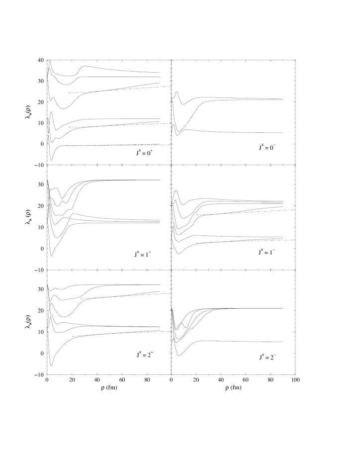
Figure 2: The lowest angular eigenvalues $\lambda_{n}$ for ⁶He (n+n+$\alpha$) as functions of $\rho$ for angular momentum and parity $J^{\pi}=0^{\pm},1^{\pm},2^{\pm}$. The solid lines are computed by numerical integration and the dot-dashed lines are the large-distance asymptotic behavior obtained from eqs.(42) and (43). The neutron-neutron interaction is from [9] and the neutron-$\alpha$ interaction is from eq.(3.1). Maximum $K$-values up to about 150 are used in the basis.

The asymptotic behavior obtained at large distance is in this case reached around 40 fm. This does not mean that all interactions produce the same results at such a distance. It means that details are unimportant, but the scattering lengths are still crucial. A larger basis would have reproduced the results of the analytical calculations up to higher $\rho$-values. However, this is not needed, because we use the asymptotic solutions as soon as they are accurate enough. This improves both accuracy and speed of the computations. The finite size of the basis gives a too fast convergence to the hyperspherical spectrum. Without an independent calculation it can therefore be difficult to assess the accuracy.

The lowest level for each $J^{\pi}$ usually contribute with the largest components of the wave function of both the possible bound state and the low-lying continuum states. For all six cases in Fig. 2 we find pockets which, except for the $0^{+}$ ground state, are unable to bind the system, but still responsible for several low-lying $S$-matrix poles as we shall see later.

The Pauli principle prohibits the core neutrons and the halo neutrons from occupying the same orbits. This has to be incorporated explicitly, since the three-body model only deals with particles without intrinsic degrees of freedom, except for their intrinsic spins. For a repulsive $s$-wave potential as described above, no bound state is present and no overlap has to be excluded. We also investigate another approximation where we use an attractive neutron-core potential with one bound $s$-state and the same scattering length and effective range. The lowest angular eigenvalue must then bend over and diverge parabolically towards $-\infty$. This corresponds at large distances to a configuration where a neutron is bound in the doubly degenerate lowest $s$-state, which is Pauli forbidden for the halo neutrons. At smaller distances the probability, or the wave function, must be small, because otherwise a significant part of the halo wave function would be inside the core, the halo and core degrees of freedom would not separate and the three-body model would not be a good approximation. The effective potential at these small distances is then rather unimportant if the model is valid. Therefore a good and inexpensive approximation to include the Pauli principle is simply to omit the lowest diverging angular eigenvalue $\lambda$ from the computations [9].

Figure 3: The lowest angular eigenvalues $\lambda_{n}$ for ⁶He (n+n+$\alpha$) as functions of $\rho$ for angular momentum and parity $J^{\pi}=0^{+}$ for the repulsive (solid) and attractive (dashed) $s$-wave potentials in eqs.(3.1) and (55). The neutron-neutron interaction is the same as in Fig. 2. The lowest diverging level for the attractive potential is omitted corresponding to our prescription for excluding the Pauli forbidden state. Maximum $K$-values up to about 150 are used in the basis.

In Fig. 3 is shown the angular eigenvalue spectrum for $J^{\pi}=0^{+}$ for both the repulsive and the attractive $s$-wave potentials in eqs.(3.1) and (55). The lowest diverging level for the attractive potential originating from zero is removed from the figure as well as from the subsequent computations. The second level for the attractive potential, originating from 12, is almost identical to the lowest level from the repulsive potential from about $\rho=1$ fm. The levels from these two potentials are remarkably similar even at smaller distances and they are completely identical in the large-distance asymptotic region. (Note that the figure only shows results up to 15 fm, where differences still can be seen.) One level originating from 32 must cross an empty region, and therefore deviate somewhat from all other levels, until it catches up with one of the levels from the other potential approaching 12 for large $\rho$. However, the lowest $\lambda$-value(s) is dominating in the wave functions of interest here and we therefore should focus on the corresponding effective potentials. The differences in these potentials are small, but in precise computations they must be compensated in one way or another. Fortunately the means for such fine tuning is already present as a three-body potential, which is different for different two-body potentials.

Table 1: The real and imaginary values $(E_{r},\Gamma)$ (in MeV) of the two lowest $S$-matrix poles $E=E_{r}-i\Gamma/2$ for ⁶He for various spins and parities. The interactions used in the upper part of the table are the same as in Fig. 4. The three-body interaction parameters are $S_{3g}=-7.55$ MeV, $b_{3g}=2.9$ fm, $S_{3g}=-31$ MeV, $b_{3g}=2.061$ fm, respectively for the first two and the last two columns. The $1^{-}$ poles in the middle are obtained with the same interactions except for an exponential shape for the three-body potential with parameters $S_{3e}=-3.11$ MeV, $b_{3e}=4.3$ fm. In the lower part of the table the repulsive potential is substituted by the attractive potential in Eq.(55). The interactions used are otherwise unchanged, except for the three-body interaction parameters, where $S_{3g}=-3.35$ MeV, $b_{3g}=3.0$ fm. The excitation energies are $E^{*}=E_{r}+0.95$ MeV, $E^{*}=E_{r}+1.54$ MeV for the left and right hand side of the table.

$J^{\pi}$	$E_{r}$	$\Gamma$	$E_{r}$	$\Gamma$	$E_{r}$	$\Gamma$	$E_{r}$	$\Gamma$
$0^{+}$	0.94	0.64	1.46	0.83	0.62	0.56	1.16	0.67
$0^{-}$	2.07	0.74	-	-	2.07	0.74	-	-
$1^{+}$	1.62	0.74	2.55	0.86	1.62	0.74	2.55	0.86
$1^{-}$	1.11	0.42	1.67	0.58	0.95	0.38	1.43	0.56
$2^{+}$	1.02	0.37	1.23	0.45	0.845	0.093	1.05	0.40
$2^{-}$	0.90	0.34	1.82	0.57	0.90	0.34	1.82	0.57
$1^{-}$	0.96	0.38	1.44	0.54
$0^{+}$	1.02	0.59	1.48	0.75
$1^{-}$	1.11	0.31	1.65	0.41
$2^{+}$	1.03	0.44	1.26	0.35

Figure 4: The total effective diagonal radial potentials for ⁶He (n+n+$\alpha$) defined in eq.(8) (solid curves) as functions of $\rho$ corresponding to the three lowest $\lambda$’s for $0^{\pm}$, $1^{\pm}$ and $2^{\pm}$. The dashed curves are the part remaining after removal of the generalized centrifugal terms, i.e. $\hbar^{2}(K+3/2)(K+5/2)/(2m\rho^{2})$, where $K(K+4)=\lambda(\rho=\infty)$ is the corresponding asymptotic hyperspherical eigenvalue. The interactions are the same as in Fig. 2 with an additional diagonal three-body interaction, i.e. $S_{3g}\exp(-\rho^{2}/b^{2}_{3g})$ with $S_{3g}=-31$ MeV, $b_{3g}=2.061$ fm, added in all partial waves, except for $J=0^{+}$ where $S_{3g}=-7.55$ MeV, $b_{3g}=2.9$ fm. The insets show the details of the lowest potentials.

For the lowest spins and parities we give in Table 1 the lowest resonance energies and the related widths obtained as $S$-matrix poles by the complex energy method. The different three-body forces in Table 1 can be considered to give the realistic range of the possible variation in the present model. In contrast, all previous computations did not produce three-body resonances in this low-energy region, except the established $2^{+}$-resonance [23, 24, 25]. For $0^{-}$, $1^{+}$ and $2^{-}$ we obtain identical poles, since the two three-body interactions only contribute at small distances where the effective two-body potentials completely dominate. On the other hand, for $0^{+}$, $1^{-}$ and $2^{+}$ we find differences of up to 0.3 MeV and 0.18 MeV for the position and the width, respectively. The systematic shifts of the positions in the right hand side of the table arise due to the slightly different $2^{+}$ energy obtained by adjusting the parameters.

The radial shape of the three-body force and the change from the repulsive to the attractive $s$-wave potential both have an effect on the lowest $S$-matrix poles. For the exponential three-body force the numerical values of positions and widths for the two lowest poles are smaller by about 0.2 MeV and 0.04 MeV, respectively. The widths are systematically smaller for the attractive potentials for $0^{+}$ and $1^{-}$ while the $2^{+}$-poles appear to depend on the individual case.

The widths of these $S$-matrix poles depend rather sensitively on their energies, which are of the same order as the height of the corresponding effective radial barriers, see Fig. 4. For these states with energies about 1 MeV, any width above 0.4 MeV corresponds to a smooth structure in the cross sections. Thus, even though the three-body interactions only amount to a fine tuning of the energies, the consequences for the presence and subsequent observation of continuum structures might be substantial.

The low-lying $S$-matrix poles seem to be rather close-lying. By a sufficiently large additional artificial three-body attraction they move down towards threshold and become eventually bound states. Their apparent energies and widths depend rather sensitively on the boundary condition introduced when the wave functions are matched to the Hankel functions at a given (large) distance $\rho_{max}$. In general the poles move towards the origin until converged with increasing $\rho_{max}$. Especially the widths are often sensitive to the matching point. They systematically decrease or sometimes remain constant with increasing $\rho_{max}$.

For the $2^{+}$-resonance the sensitivity is very small when $\rho_{max}$ is larger than 40 fm. Most of the other poles, however, require larger $\rho_{max}$ indicating that they are somewhat more related to the larger distances in hyperradius. This might be a reminiscence of the Efimov effect, where the bound states are pushed up into the continuum, but still with a relatively low-lying and dense energy spectrum. The Efimov effect would arise as the consequence of very low-lying two-body virtual $s$-states in the neutron-core and the neutron-neutron subsystems. The actual parameters give energies of about –200 keV for these virtual $s$-states.

The main part of the radial wave function is determined by the angular momentum dependent effective potential corresponding to the lowest $\lambda$. We show these potentials for $0^{\pm}$, $1^{\pm}$ and $2^{\pm}$ in Fig. 4, where we also exhibit the parts remaining after removal of the generalized centrifugal barrier terms, i.e. $\hbar^{2}(K+3/2)(K+5/2)/(2m\rho^{2})$, where $K(K+4)=\lambda(\rho=\infty)$ is the corresponding asymptotic hyperspherical eigenvalue. As for two-body systems this remaining part is more revealing than the total potential, which could be repulsive for all $\rho$ and still produce a resonance provided a sufficiently strong attractive pocket is present in this “non-centrifugal” part of the potential.

The pocket in the effective radial potential is absent for angular momentum $0^{-},1^{\pm}$ and $2^{-}$. The pocket for $2^{+}$, which definitely produces a narrow resonance at about 1 MeV, is slightly less pronounced than for $0^{+}$, where a bound state at about 1 MeV is present. All the lowest effective potentials are attractive without the “centrifugal barrier” and therefore they could give rise to resonances.

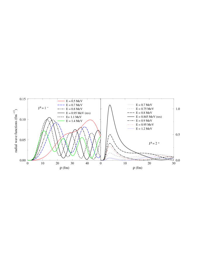
Figure 5: The absolute values of the radial wave functions for ⁶He (n+n+$\alpha$) after diagonalization as functions of $\rho$ for real energies in intervals around the real parts of the $S$-matrix poles $E_{r}=0.95$ MeV for $1^{-}$ and $E_{r}=0.845$ MeV for $2^{+}$. Only the dominating component in the full computation is shown. The interactions are the same as in Fig. 4.

The observables are related to real values of the energy. We therefore solve the radial equations on the real axis for energies corresponding both to the real values of the $S$-matrix pole and to values away from this pole. We show in Fig. 5 the absolute values of these wave functions for $1^{-}$ and $2^{+}$. The peak at small distance is narrower and much more pronounced for $2^{+}$ than for $1^{-}$. Still for $1^{-}$, a substantial amount of strength is present between 5 fm and 20 fm whenever the energy is within the width of the $S$-matrix pole. Outside the widths of all the poles the wave functions appear with very little probability at distances below 15 fm, see the curve for $1^{-}$ with the energy 1.4 MeV.

We have $2^{+}$ as a pronounced resonance and $1^{-}$ which only shows up as a much smaller and broader peak in Fig. 5. These wave functions reflect the effects on the real axis of the properties of the corresponding complex $S$-matrix poles. For other energies and angular momenta a similar picture is found. The small distance enhancements are obtained whenever the energy is within the width from the energy of an $S$-matrix pole. These poles therefore produce observable effects. However, the size of the effects depends on both the detailed properties of the poles and the precise definition of the observable. It is also clear from Fig. 5 that contributions from $S$-matrix poles may continuosly vary from substantial to vanishing small.

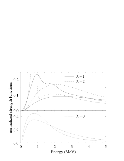
Figure 6: The strength functions, $dB_{E\lambda}/dE=\sum_{n}\left|\langle nJ^{\pi}||M(E\lambda)||0^{+}\rangle\right|^{2}$ for ⁶He (n+n+$\alpha$) as functions of energy for transitions from the ground state to $0^{+}$ (dotted), $1^{-}$ (solid) and $2^{+}$ (dashed) excited continuum states. The operator is $M(E\lambda,\mu)=\rho^{2}$ and $\sum_{i=1}^{3}eZ_{i}r_{i}^{\lambda}Y_{\lambda\mu}(\hat{r}_{i})$ respectively for $\lambda=0$ and $1,2$. The units are the corresponding sum rule values $\langle 0^{+}|\rho^{4}|0^{+}\rangle-\langle 0^{+}|\rho^{2}|0^{+}\rangle^{2}$ for $\lambda=0$ and $e^{2}Z_{\alpha}^{2}(2\lambda+1)\langle 0^{+}|r_{\alpha}^{2\lambda}|0^{+}\rangle/(4\pi)$ for $\lambda=1,2$, where $eZ_{\alpha}$ is the ⁴He-charge and $r_{\alpha}$ is the ⁴He-distance from the ⁶He center of mass. The interactions are the same as in Fig. 4. The smooth curves (smaller at small distance) correspond to plane waves for the continuum states.

3.3 Strength functions and Coulomb cross sections

The continuum structure can be investigated by electromagnetic and/or nuclear excitations from the ground state. These transitions are described by observables such as the multipole strength functions. The lowest and most important three of these are shown in Fig. 6 as functions of energy both for plane waves and for the proper continuum wave functions. The curves are normalized by their respective sum rule values and each of them would therefore after integration over all energies give 1. The strengths below 10 MeV are 97%, 78% and 83% for $\lambda=0,1,2$, respectively and for the corresponding plane waves we obtain the somewhat smaller values 94%, 60% and 81% obtained.

The influence of the final state interaction is directly reflected in deviations from the broader plane wave distributions. In general we always must have a rise from zero to a maximum and a fall off towards zero at large energy. Especially pronounced peak structure as observed for $\lambda=2$ is the signature of a resonance, which in this case reflects the well known $2^{+}$ state at 0.82 $\pm$ 0.025 MeV of width 0.113 $\pm$ 0.020 MeV [49], which in this computation appears at 0.82 MeV with the width 0.093 MeV.

For $1^{-}$ a peak and a shoulder appears at about 0.95 MeV and 1.8 MeV. This $1^{-}$ enhancement at low energy arises from the two overlapping $S$-matrix poles seen in Table 1, see also [26]. The enhancement almost coincides in energy with the dominating $2^{+}$-peak and consequently it must be harder to detect experimentally. The nuclear $0^{+}$ strength function resembles the plane wave result more than the higher multipoles reflecting broader underlying structures where the poles have larger widths if present at all.

Figure 7: The dipole and quadrupole (inset) contribution to the differential Coulomb dissociation cross section of ⁶He (n+n+$\alpha$) at 800 MeV/nucleon as function of the three-body energy for a Cu- and a Pb-target. The Cu-results are multiplied by $(82/29)^{2}$ to remove the dominating, but trivial overall charge scaling. The energy of the ⁶He-beam is 800 MeV/nucleon. The interaction is the same as in Fig. 4. On the right hand side is shown the strength functions $dB_{E1}/dE$ for the attractive potential in eq.(55) (dashed) and for the repulsive $s$-wave potential in eq.(3.1) (solid and dot-dashed) with gaussian (G) and exponential (E) three-body interactions. The parameters are given in section 3.

The differential Coulomb dissociation cross section is now computed by multiplication of strength functions and virtual photon spectra. The results are shown in Fig. 7 for Pb and Cu targets for both dipole and quadrupole excitations. As expected the dipole contribution has a width of about 2 MeV and it is by far dominating in absolute size. The quadrupole distribution is much smaller, but strongly peaked at the resonance energy. The target dependence vary with the square of the target charge as seen from eq.(50). Both potentials as well as different three-body interactions give similar, but distinguishable results as seen in the right hand side of Fig. 7. The major differences arise from the difference in the ground state structure, in particular the larger spatial extension found for the exponential three-body force. With the same ground state wave function almost identical strength functions would appear.

Previous computations of $1^{-}$-strength functions reported peaks at about 2.5 MeV and shoulders at about 6 MeV [20, 23, 25, 50]. The present $1^{-}$-strength function differs substantially with much more strength at low energies indicating contributions from larger distances. Unfortunately corresponding experiments are so far not available for ⁶He.

The low-energy enhancement of the dipole strength function move strength towards energies with larger values of the number of virtual photons. The total Coulomb dissociation cross section is therefore larger than that obtained with plane waves in the final state. It is also necessarily large compared to analogous cross sections for ordinary nuclei, again due to a relatively large low-energy enhancement. This is explained physically as the result of the weakly bound neutrons easily separated by a small Coulomb disturbance.

The total Coulomb dissociation cross section is simply obtained by integrating the differential cross section over energy. The quadrupole contribution amounts here to about 0.5% and the total cross section is 373 mb and 54 mb for the two targets and the beam energy of 800 MeV/A. This is in agreement with the experimental extrapolation of [51] and the calculated values in [22] while somewhat larger than computed in [52]. This rather favorable comparison supports the three-body model with a substantial $1^{-}$ low-energy enhancement. However, the enhancement is not in itself proof of the presence of a low-lying three-body dipole resonance. Any attraction would produce more strength at low energies. A resonance needs more than marginal attraction. Furthermore, the enhancement could be due to relatively strong underlying two-body structures. In the present case the $S$-matrix pole at about 1 MeV could indicate a resonance, which however overlaps the next pole at about 1.5 MeV. This in turn results in the relatively weak peak in the wave function at small distances in Figs. 5 and 6.

Figure 8: The total Coulomb dissociation cross section as function of the laboratory energy for a ⁶He-beam colliding with a ²⁰⁸Pb-target. Both the quadrupole part and the total cross sections are shown. The plane wave results are shown as dashed curves. The interaction is the same as in Fig. 4. The experimental point is from [51].

The total Coulomb dissociation cross section is shown in Fig. 8 as function of beam energy. Both dipole and quadrupole contributions are shown. The experimental point from [51] has very large error bars and therefore not surprisingly in agreement with the computations. At high energy we find a slightly decreasing function with values about a few hundred mb. At energies below about 10 MeV/A the cross section drops dramatically with decreasing energy. Although the approximations are dubious at these energies the precise behavior of this rapid change of the cross section should be sensitive to the details of the halo structure.

4 The ¹¹Li-system as n+n+⁹Li

The $\alpha$-particle has spin zero and the neutron-$\alpha$ system has a low-lying $p$-resonance. Consequently ⁶He has spin zero and consists mainly of $p^{2}$-configurations of the neutron-$\alpha$ relative wave function. For ¹¹Li the spin and parity is $\frac{3}{2}^{-}$ as for the ⁹Li-core of the three-body system. Furthermore the neutron-⁹Li system has apparently a virtual $s$-states at about –200 keV and somewhat higher-lying $p$-resonances at about 600 keV [13, 53]. Consequently ¹¹Li is expected to consist of dominating $s^{2}$-configurations of the relative neutron-⁹Li wave function. The details about the two-body subsystems are not accurately known, but already the possibility of low-lying $s$-states is interesting, since the conditions for the Efimov effect then nearly are fulfilled. In this section we shall therefore use the knowledge obtained from the simpler and better known ⁶He and predict the more uncertain properties of ¹¹Li.

4.1 Interactions and numerical details

The neutron-neutron interaction is the same as used in the previous computations for ⁶He. The neutron-core effective interaction often assumes zero spin for both ⁹Li and ¹¹Li although the correct spins are $\frac{3}{2}$ for both nuclei. The spin-orbit term ${\bf\ell}\cdot{\bf s}_{n}$ for a neutron in the relative motion around a spin-zero core is used although the natural generalization, which in fact has been used previously [9, 54], would be of the form ${\bf\ell}\cdot({\bf s}_{n}+{\bf s}_{c})$ for finite core spin $s_{c}\neq 0$.

However, in our case of nuclear clusters the Pauli principle must be treated in one way or another. This can be achieved either by a large repulsion in forbidden states or by omitting or projecting out the forbidden configurations. These different approximations assume that the forbidden states can be identified and preferentially expressed in terms of the three-body wave functions obtained as solutions for the corresponding neutron-core potential. Thus an effective two-body potential is much easier to apply in three-body computations when its symmetries, quantum numbers and the related eigenfunctions are expressed by the quantities used in calculations of the nucleonic motion inside the core. We shall therefore use the mean-field spin-orbit form ${\bf\ell}\cdot{\bf s}_{n}$, where the spin of the core does not enter.

In the present work we shall deal with the Pauli principle in several ways and then compare the results. The neutrons in the core occupy the lowest $s_{1/2}$ and $p_{3/2}$-states. The occupied $p_{3/2}$-state is avoided in the three-body computation by using a sufficiently large repulsive two-body potential. The neutron-⁹Li $s$-wave potential is either shallow without any bound states or deeper with one bound state but the same scattering length and effective range. In the latter case the forbidden three-body configuration is excluded in the calculations [9].

Another qualitative difference from the zero core-spin computations is the two possible couplings of the spins of the neutron and the core. For the neutron-⁹Li the total spin can then be 1 or 2. In general we therefore also include a spin-spin potential term to differentiate between these two spin-couplings for each orbital angular momentum state. Such spin-splitting terms are most likely present due to the strong spin dependence of the underlying basic interaction and consequently hard to ignore.

For finite core spin the interactions corresponding to a shallow $s$-wave potential are

$$V_{nc}^{(\ell=0)}=(-7.28-0.31{\bf s}_{n}\cdot{\bf s}_{c})\exp(-r^{2}/2.55^{2})$$

$$V_{nc}^{(\ell=1)}=\left(18.25+1.47{\bf s}_{n}\cdot{\bf s}_{c}+55{\bf\ell}\cdot{\bf s}_{n}\right)\exp(-r^{2}/2.55^{2})\;.$$ (56)

The two $s$-wave scattering lengths and effective ranges are (7.65 fm, 4.53 fm) and (10.88 fm, 4.77 fm) corresponding to virtual $s$-states at $-0.247$ MeV and $-0.140$ MeV for the total spin of 1 and 2, respectively. The energies and widths of the $p_{1/2}$-resonances defined as a poles of the $S$-matrix are $E(p_{1/2})=0.75$ MeV, $\Gamma(p_{1/2})=0.87$ MeV and $E(p_{1/2})=1.60$ MeV and $\Gamma(p_{1/2})=3.74$ MeV, respectively for spin 1 and 2. In all cases the high-lying $p_{3/2}$-resonance is not contributing in the three-body calculations and the Pauli blocking by the core neutrons are simulated in this way.

In addition to the two-body potentials a diagonal three-body force could be introduced for fine tuning as for ⁶He. However, the idea of using the three-body force is to include effects beyond those accounted for by the two-body interactions and too imprecise and too little information is available about this neutron-core system. It is therefore at the moment as reasonable to adjust the two-body interaction instead of adding another uncertainty at this level.

The choice of interaction parameters is dictated by the knowledge of ¹¹Li and the accumulating information about the structure of ¹⁰Li, i.e. a $p$-resonance at about 0.6 MeV, a low-lying virtual $s$-state and a small spin splitting of these states [13, 53]. We obtain a three-body energy of about –300 keV reproducing the ¹¹Li-binding energy of 295 $\pm$ 35 keV with the corresponding root mean square radius of 3.34 fm. Furthermore, the calculated fragment momentum distributions in ¹¹Li break-up reactions also compare rather well with measured values [9]. Then the ¹¹Li ground state wave function has about 80% and 20% of $s^{2}$ and $p^{2}$-configurations, respectively.

We shall use this “realistic” interaction in the investigation of the continuum properties of ¹¹Li. All possible $s$- and $p$-waves are included. When the large-distance asymptotic behavior is reached the solutions are obtained from eqs.(24) and (27). The radial equations are integrated from zero to about 200 fm. Further arguments for these numerical choices can be found in [26].

Figure 9: The lowest angular eigenvalues $\lambda_{n}$ for ¹¹Li (n+n+⁹Li) as functions of $\rho$ for angular momentum $J^{\pi}=\frac{1}{2}^{\pm},\frac{3}{2}^{\pm},\frac{5}{2}^{\pm}$. The dot-dashed lines are the large distance asymptotic behavior from eq.(20). The neutron-neutron interaction is from [9] and the neutron-⁹Li interaction is given in eq.(4.1). Maximum hyperspherical quantum numbers up to about 100 are used.

4.2 Solutions and $S$-matrix poles

The angular eigenvalues for $\frac{1}{2}^{\pm}$, $\frac{3}{2}^{\pm}$ and $\frac{5}{2}^{\pm}$ are shown in Fig. 9 together with the asymptotic behavior obtained from the analytical expressions. For the ground state with $\frac{3}{2}^{-}$ we find the two lowest levels very similar to the spectrum for zero core-spin. However, now a series of additional higher-lying levels appear. They arise from the broken symmetries due to the finite core spin $\frac{3}{2}$.

The spectra contain almost identical levels for $\frac{1}{2}^{+}$, $\frac{3}{2}^{+}$ and $\frac{5}{2}^{+}$ as well as for $\frac{1}{2}^{-}$, $\frac{3}{2}^{-}$ and $\frac{5}{2}^{-}$. A number of additional levels are furthermore present for $\frac{3}{2}^{\pm}$. The corresponding degeneracy is due to the weak neutron-core spin-splitting potential. It can be explained by coupling two neutrons in $s_{1/2}$ and $p_{1/2}$ neutron-core states to $0^{\pm}$ and $1^{-}$ which in turn, coupled to the $\frac{3}{2}^{-}$ from the ⁹Li-core, results in sets of nearly degenerate $\frac{3}{2}^{\pm}$ and $\frac{1}{2}^{+}$, $\frac{3}{2}^{+}$, $\frac{5}{2}^{+}$-states. The lowest $\frac{1}{2}^{-}$, $\frac{5}{2}^{-}$-states arise from couplings of higher orbitals.

Table 2: The real and imaginary values $(E_{r},\Gamma)$ (in MeV) of the lowest $S$-matrix poles $E=E_{r}-i\Gamma/2$ for ¹¹Li for various spins and parities $J^{\pi}$. The excitation energy $E^{*}=E_{r}+0.305$ MeV. The interactions for the upper part of the table are the same as in Fig. 1. The middle of the table contains the results for a model with $s_{c}=0$ and the same average positions of the lowest neutron-core resonances. i.e. an average energy of the $s_{1/2}$ virtual state and the $p_{1/2}$-resonance at -0.18 MeV and 1.22 MeV, respectively. The lower part of the table is for a with one Pauli forbidden $s$-state. The $s_{1/2}$ virtual state is at -0.18 MeV and the $p_{1/2}$ neutron-core resonance is at 0.50 MeV.

$J^{\pi}$	$E_{r}$	$\Gamma$	$E_{r}$	$\Gamma$	$E_{r}$	$\Gamma$	$E_{r}$	$\Gamma$	$E_{r}$	$\Gamma$
$\frac{1}{2}^{-}$	-	-	-	-	1.37	0.51	1.56	0.56	1.98	0.65
$\frac{3}{2}^{-}$	-0.305	0	0.89	0.43	1.41	0.56	1.60	0.61	2.03	0.68
$\frac{5}{2}^{-}$	-	-	-	-	1.36	0.49	1.60	0.68	2.01	0.72
$\frac{1}{2}^{+}$	0.65	0.35	-	-	1.28	0.48	1.74	0.64	1.95	0.68
$\frac{3}{2}^{+}$	0.68	0.33	0.88	0.33	1.33	0.50	1.77	0.63	2.08	0.71
$\frac{5}{2}^{+}$	0.68	0.37	-	-	1.36	0.55	1.74	0.64	2.11	0.84
$0^{+}$	-0.307	0	1.00	0.37	1.35	0.45	1.62	0.61	1.96	0.92
$1^{+}$	-	-	-	-	1.40	0.59	1.59	0.63	2.02	0.81
$0^{-}$	-	-	0.92	0.39	1.25	0.51	1.82	0.62	2.02	0.65
$1^{-}$	0.64	0.31	-	-	1.46	0.53	1.76	0.59	2.08	0.67
$0^{+}$	-0.306	0	1.00	0.31	1.40	0.41	1.64	0.56	1.99	0.88
$1^{+}$	-	-	-	-	1.37	0.49	1.62	0.58	2.03	0.75
$0^{-}$	-	-	0.88	0.30	1.29	0.43	1.76	0.53	1.96	0.69
$1^{-}$	0.64	0.27	-	-	1.50	0.39	1.82	0.60	2.00	0.71

For the lowest spins and parities we give in Table 2 the lowest resonance energies and the related widths obtained as $S$-matrix poles by the complex energy method. We show the results for core-spins zero with shallow and deep potentials and for the spin $\frac{3}{2}$. The spin-zero core approximation show a low-lying and relatively narrow $S$-matrix pole for $1^{-}$, $0^{-}$ and perhaps also for $0^{+}$ while we find nothing similar for $1^{+}$. Higher-lying and broader poles are found for all angular momenta and parities. The same structure is found for the deep potential. The shallow and deep potentials also quantitatively give very similar results.

With the correct finite core spin the symmetries are broken. We recognize the three times nearly degenerate $1^{-}$-pole at about 0.65 MeV with a width of about 0.35 MeV. We also find degenerate $0^{\pm}$ $S$-matrix poles at 0.89 MeV with widths of 0.33 MeV and 0.43 MeV. More discussion about these poles can be found in [26].

The relatively large number of $S$-matrix poles could be due to the Efimov effect, which occurs when the scattering lengths are much larger than the range of the interactions [32, 38]. With increasing scattering lengths, the infinitely many poles of the three-body $S$-matrix move towards the point $E$=0. For very large but finite scattering lengths a number of poles must already appear close to zero. These poles originate from the long distance tail of the effective potential ($\propto\sum_{i=1,3}{a_{i}}\mu_{jk}^{-1}\rho^{-3}$, where $a_{i}$ is the scattering length of the $i$-th subsystem) and they are not sensitive to the details of the interactions. Since there are no confining barriers for these poles, their corresponding widths must be rather large.

For ¹¹Li the Efimov condition is almost fulfilled, since $a_{nn}\mu_{nn}^{-1}+2a_{cn}\mu_{cn}^{-1}\approx$50 fm. This must necessarily result in a number of broad $S$-matrix poles near the $E$=0 point. For ⁶He there is a low-lying two-body $p_{3/2}$-resonance while for ¹¹Li there is instead an $s_{1/2}$-virtual state. The latter case is therefore closer to the Efimov conditions and a larger number of low-lying three-body $S$-matrix poles could be expected.

An indication of the properties and origin of these $S$-matrix poles is obtained by matching the radial wave functions at various decreasing values of $\rho_{max}$. The poles move towards larger absolute values of the energies for decreasing matching radii. The imaginary values stay almost constant for the lowest $0^{+}$ and $1^{-}$-states indicating resonance-like structures. Both imaginary and real values increase for the other poles.

Figure 10: The total effective diagonal radial potential (solid curves) as functions of $\rho$ corresponding to the four lowest $\lambda$’s for $J^{\pi}=\frac{1}{2}^{\pm},\frac{3}{2}^{\pm},\frac{5}{2}^{\pm}$ for ¹¹Li (n+n+⁹Li). The dashed curves are the part remaining after removal of the generalized centrifugal terms, i.e. $\hbar^{2}(K+3/2)(K+5/2)/(2m\rho^{2})$, where $K(K+4)=\lambda(\rho=\infty)$ is the corresponding asymptotic hyperspherical eigenvalue. The interactions are as in Fig. 9. The insets show the details of the lowest potentials.

The lowest effective adiabatic potentials determine the radial wave function and the energy of possible bound states. They are shown in Fig. 10 for various spins and parities. In all cases we find attractive potentials around 50 MeV deep after removal of the repulsive centrifugal barriers. Resonances are therefore possible in all these channels. With the centrifugal barriers all the potentials are still attractive except those corresponding to $\frac{1}{2}^{-}$ and $\frac{5}{2}^{-}$. The ground state of $J^{\pi}=\frac{3}{2}^{-}$ exhibits the largest attractive pocket and no barrier for the lowest adiabatic potential and a barrier height of 1.7 MeV at about 7 fm for the second potential. The $1^{-}$ excited states all have attractive pockets as well as repulsive barriers of about 0.6-0.9 MeV for $\rho$ between 10 and 15 fm.

Compared to $0^{+}$ of ⁶He we have now a less attractive but broader $\frac{3}{2}^{-}$-potential corresponding to the ground state quantum numbers, see Fig. 4. The $1^{-}$ excited states for ⁶He have no attractive pocket while it is substantial for ¹¹Li in agreement with the calculated low-lying $S$-matrix poles, which appear around the barrier height.

Figure 11: The absolute values of the radial wave functions for ¹¹Li (n+n+⁹Li) as functions of $\rho$ for real energies in an interval around the real part of the $S$-matrix pole $E_{r}=0.68$ MeV for $\frac{3}{2}^{+}$. The interactions are the same as in Fig. 9.

The wave functions corresponding to real energies around the real part of the pole energy 0.68 MeV are shown in Fig. 11. For energies below 0.68 MeV and outside its width the peak moves to larger distances, but remains of comparable size. For the energy 0.8 MeV we find a similar peak at a slightly smaller distance. This peak can be viewed as the combined effect on the real axis of the two overlapping pole structures at 0.68 MeV and 0.88 MeV, see Table 2. For 1.0 MeV, respectively within and outside the widths of the poles at 0.88 MeV and 1.33 MeV, the peak has decreased and moved to a smaller distance. None of all these peaks are pronounced in comparison with the next peaks of the same wave function. Thus strong $1^{-}$-resonance structures are not obtained.

Figure 12: The strength functions $dB_{E\lambda}/dE\propto\sum_{n}\left|\langle nJ^{\pi}||M(E\lambda)||J_{0}^{\pi_{0}}\rangle\right|^{2}$, $M(E\lambda,\mu)$ = $\sum_{i=1}^{3}eZ_{i}r_{i}^{\lambda}Y_{\lambda\mu}(\hat{r}_{i})$, for ¹¹Li (n+n+⁹Li) as function of energy for transitions from the ground state via $0^{+}$ to $\frac{3}{2}^{-}$ (left hand side), via $1^{-}$ (right hand side) to $\frac{1}{2}^{+}$, $\frac{3}{2}^{+}$ and $\frac{5}{2}^{+}$ excited continuum states. The smooth curves (smaller at small distance) correspond to plane waves for the continuum states. The curves are normalized to the corresponding sum rule values given in Fig. 6. The interactions are the same as in Fig. 9.

4.3 Strength functions and Coulomb cross sections

The dominating dipole term in electromagnetic excitations can excite the ground state to continuum states of $J^{\pi}=\frac{1}{2}^{+},\frac{3}{2}^{+},\frac{5}{2}^{+}$ while the nuclear monopole excitation only produce $\frac{3}{2}^{-}$-states. The corresponding calculated strength functions are shown in Fig. 12 together with the results obtained by using plane waves for the continuum wave functions. The monopole strength resembles the results of the plane wave computation in agreement with the lack of low-lying $S$-matrix poles below 0.8 MeV, see Table 2. The dipole strengths are almost proportional to the statistical weights of $(2J+1)$ and all of them are enhanced significantly above the plane wave results at low energies. This enhancement overlaps with the position of the lowest $1^{-}$-poles in Table 2.

Figure 13: The strength functions $dB_{E\lambda}/dE=\frac{1}{2J_{0}+1}\sum_{nJ^{\pi}}\left|\langle nJ^{\pi}||M(E\lambda)||J_{0}^{\pi_{0}}\rangle\right|^{2}$, $M(E\lambda,\mu)=\sum_{i=1}^{3}eZ_{i}r_{i}^{\lambda}Y_{\lambda\mu}(\hat{r}_{i})$, for $\lambda=1$ for ¹¹Li (n+n+⁹Li) as function of energy. The smooth curves correspond to plane waves for the continuum states. The interactions are the same as in Table 2 for $s_{c}=0$ and Fig. 9 for $s_{c}=\frac{3}{2}^{-}$ except for the JJH curve obtained with the potential in [45]. The experimental points are from [13, 14, 15]. The arbitrary units in [15] are normalized to our sum rule value, while the absolute data from [13, 14] are left unchanged.

The total dipole strength function, where the contributions from all $J^{\pi}$ in the continuum are added, is in Fig. 13 compared to the zero core approximation and the three available measured distributions. The plane wave result are the same for zero and finite core spin, because the ground state essentially is unchanged. The interaction with zero core-spin gives a distribution shifted about 100 keV towards lower energy compared to the result for the realistic full computation. A lower and broader peak is obtained for the potential from [45] where the $p^{2}$-content of the three-body wave function is very small. The low-lying $1^{-}$-poles around 0.65 MeV enhance the strength functions at low energies compared to the plane wave results.

The computed strength functions substantially exceed most of the data points [13, 14, 15] in the peak region around 0.55 MeV. (Note however that the data in [13, 14] contain much less total strength.) A reduction could be achieved with higher energy and larger width of the $S$-matrix pole, but this would probably only be provided by a potential with much too small $p^{2}$-content in the three-body wave function. It is also a curious fact that other models provide $1^{-}$ strength functions substantially closer although not in complete agreement with the data [21, 55, 56]. This is of course related to the lack of low-energy $1^{-}$-resonances or $S$-matrix poles in these computations.

In this context it is worth pointing out that it is difficult to find the most appropriate comparison with the different experimental results in the figure. The normalization must be properly chosen and the theoretical results must be folded with the distributions (unknown to us) related to the equipment used in the different experiments.

Figure 14: The dipole approximation (solid curve) to the Coulomb dissociation cross section of ¹¹Li as function of laboratory energy per nucleon for a Pb-target. The plane wave results are the dashed curve. The interactions are the same as in Fig. 9. The data point is from [13].

The strength functions rise from zero to a maximum and then fall off towards zero at large energy whereas the virtual photon spectra decrease monotonically with excitation energy [44]. The low-energy enhancement necessarily implies a larger Coulomb cross section, since the dipole is the dominating dissociation mode. We show in Fig. 14 computed total cross sections as function of beam energy for a ¹¹Li projectile on a lead target. The only available data point with relatively large error bars is in agreement with the computation [13], but substantially larger than the plane wave result. For 280 MeV/A we find 1458 mb and 1501 mb, respectively for the potentials with zero core-spin and with a small $p^{2}$-content of the wave function.

The cross section decreases at large beam energy due to the similar decrease of the virtual photon spectrum. At small energy, where the approximations are invalid, we find an increasing cross section due to the low-energy cut-off of the strength function by the virtual photon spectrum. At the maximum around 5 MeV per nucleon this and other reactions are expected to be sensitive to the details of the neutron halo structure.

5 Summary and conclusions

Borromean halo systems are almost by definition weakly bound and excited states are usually entirely absent. The continuum is therefore easy to excite and unavoidable in descriptions of essentially all reactions involving such particles. The spatial extention of the bound state and the small binding energy require rather accurate treatment of the large distances. A suitable method was recently developed and applied to compute the ground state of halo systems. This method is in the present paper extended to apply for the low-energy part of the three-body continuum.

The Faddeev equations in coordinate space are solved in two steps. First the discrete spectrum of the angular part is computed and used as a complete basis set. Then the coupled set of radial equations is solved with the appropriate continuum wave boundary conditions. The angular equations for large distances outside the short ranges of the potentials are especially simple. However, they are essential and therefore treated carefully.

The three Faddeev components are very useful in the detailed description of the particle correlations. We show that only the three $s$-waves (one in each component) for a given total orbital angular momentum couple at large distances. All other partial waves are decoupled. We therefore solve these much smaller and simpler sets of coupled and uncoupled angular equations at large distances. Some of these asymptotic solutions are obtained analytically and others as solutions to trancendental analytical equations. As a necessary intermediate result we derive a convenient expression for the transformation of angular functions between two different Jacobi coordinate systems.

Systems with two identical neutrons and a core of finite spin are specifically treated. The continuum spectra of the two Borromean halo nuclei ⁶He (n+n+$\alpha$) and ¹¹Li (n+n+⁹Li) are investigated numerically in some detail. Two-body interactions with and without bound states, but reproducing the observed low-energy scattering data are used for ⁶He. In addition three-body interactions with several radial shapes are added to obtain the measured binding energy. For ¹¹Li no three-body interaction is used, since the two-body interaction is unknown and therefore directly parametrized to reproduce anticipated two-body resonances and virtual states in addition to the momentum distributions in fragmentation reactions.

The antisymmetry between the neutrons in the halo and in the core is accounted for in two ways. First by using a repulsive or a shallow neutron-core potential without bound states. Second by omitting the lowest adiabatic potential arising from a more attractive neutron-core potential with one bound state from the set of radial equations. The results are compared.

The adiabatic potentials are decisive for the radial solutions. The lowest potential in each channel is attractive when the corresponding generalized centrifugal barrier is removed. All channels are therefore potentially able to support resonance-like structures. The pocket in the adiabatic radial potential is absent for ⁶He for angular momentum $0^{-},1^{\pm}$ and $2^{-}$ and well developed for both $0^{+}$ and $2^{+}$. For ¹¹Li the adiabatic potentials for $1^{-}$-excitations all have attractive pockets and effective barriers of $0.75\pm 0.15$ MeV. Also the $0^{+}$-channel has a well developed attractive pocket, but no barrier, for the lowest potential supporting the ground state. The second potential for $0^{+}$-excitations is also attractive with a barrier of about 1.7 MeV.

We calculate the $S$-matrix poles by the complex energy method. The lowest of these poles appear slightly above the barriers and their widths are consequently relatively large and rather sensitive to fine tuning of the interactions. One exception is the known narrow $2^{+}$-resonance in ⁶He which is reproduced in the calculation. The narrowest low lying poles for ⁶He appear for $1^{-}$ and $2^{-}$ at about 1 MeV with widths of 0.3-0.4 MeV. For ¹¹Li they appear for $1^{-}$ and $0^{\pm}$ respectively at about 0.65 MeV and 0.9 MeV with widths of about 0.35 MeV. The unusually many low-lying $S$-matrix poles could indicate that the Efimov limit is fairly close.

We computed the electric excitations from ground to continuum states. The strength functions are rather strongly enhanced at low energies due to the low-lying $S$-matrix poles. The functions extracted from measurements for ¹¹Li are apparently significantly smaller than our computations. On the other hand the same experimental information agrees with the computed Coulomb cross section. A proper consistent comparison is still lacking. Also for ⁶He we obtain enhanced dipole strength functions at low energies. Here the experimental information is not available, but the observed $1^{-}$-resonance is reproduced almost within the experimental uncertainties. We have not attempted to reproduce this somewhat controversial resonance more precisely.

In conclusion, we have developed a method to solve the three-body problem for short-range potentials. The method treats with special care the large distances which are essential for the spatially extended halo systems. We investigate the continuum spectra for the two halo nuclei ⁶He and ¹¹Li and find a number of low-lying $S$-matrix poles. Strength functions are computed and compared with other calculations and available experimental data. Various disagreements are pointed out and several controversial features are exhibited.

Acknowledgments.

We thank E. Garrido and E. Nielsen for help and continuos discussions. One of us (A.C.) acknowledges the support from the European Union through the Human Capital and Mobility program contract nr. ERBCHBGCT930320.

Appendix A
Rotations between different sets of Jacobi coordinates
We want to “rotate” the wave function from one set of Jacobi coordinates to another set as defined in eq.(2.2). Only the leading order in an expansion in $1/\rho$ is needed. We must then first express $({\bf x}_{j},{\bf y}_{j})$ in terms of $({\bf x}_{i},{\bf y}_{i})$. The six-dimensional transformation is [57, 58]

$${\bf x}_{j}=-{\bf x}_{i}\cos\varphi_{k}+{\bf y}_{i}\sin\varphi_{k}\;\;,\;\;{\bf y}_{j}=-{\bf x}_{i}\sin\varphi_{k}-{\bf y}_{i}\cos\varphi_{k}$$ (1)

where $\varphi_{k}$ is defined in eq.(18). Defining the angle $\gamma$ between ${\bf x}_{i}$ and ${\bf y}_{i}$ by

$$\cos\gamma\equiv{{\bf x}_{i}\cdot{\bf y}_{i}\over x_{i}y_{i}}\;,$$ (2)

we have the relation between the hyperangles $\alpha_{i}$ and $\alpha_{j}$ related to the two coordinates

$$\sin^{2}\alpha_{j}=\cos^{2}\varphi_{k}\sin^{2}\alpha_{i}+\sin^{2}\varphi_{k}\cos^{2}\alpha_{i}+2\cos\varphi_{k}\sin\varphi_{k}\sin\alpha_{i}\cos\alpha_{i}\cos\gamma\;.$$ (3)

We now expand the following function, related to the function in eq.(2.2), of $\alpha_{j}$ in terms of Legendre polynomials $P_{\ell}(\cos\gamma)$:

$$\frac{\phi_{n\ell_{x}^{\prime}\ell_{y}^{\prime}Ls_{x}^{\prime}S}^{(j)}(\alpha_{j})}{\sin(2\alpha_{j})\sin^{\ell_{x}^{\prime}}\alpha_{j}\cos^{\ell_{y}^{\prime}}\alpha_{j}}=\sum_{\ell}A_{\ell}^{\ell_{x}^{\prime}\ell_{y}^{\prime}L}(\alpha_{i})P_{\ell}(\cos\gamma)\;,$$ (4)

$$A_{\ell}^{\ell_{x}^{\prime}\ell_{y}^{\prime}L}(\alpha_{i})\equiv{2\ell+1\over 2}\int d\cos\gamma{\phi_{n\ell_{x}^{\prime}\ell_{y}^{\prime}Ls_{x}^{\prime}S}^{(j)}(\alpha_{j})\over\sin(2\alpha_{j})\sin^{\ell_{x}^{\prime}}\alpha_{j}\cos^{\ell_{y}^{\prime}}\alpha_{j}}P_{\ell}(\cos\gamma)\;,$$ (5)

where $\alpha_{j}$ is the function of $\alpha_{i}$ and $\gamma$ defined through eq.(A3). Then changing the integration variable from $\cos\gamma$ to $\alpha_{j}$, i.e.

$$d\cos\gamma={\sin(2\alpha_{j})\over\sin(2\alpha_{i})}{2\over\sin(2\varphi_{k})}d\alpha_{j}\;,$$ (6)

we can rewrite eq.(A5) as

$$A_{\ell}^{\ell_{x}^{\prime}\ell_{y}^{\prime}L}(\alpha_{i})={2\ell+1\over\sin(2\varphi_{k})\sin(2\alpha_{i})}\int_{|\varphi_{k}-\alpha_{i}|}^{\pi/2-|\pi/2-\varphi_{k}-\alpha_{i}|}d\alpha_{j}$$

$$\times{\phi_{n\ell_{x}^{\prime}\ell_{y}^{\prime}Ls_{x}^{\prime}S}^{(j)}(\alpha_{j})\over\sin^{\ell_{x}^{\prime}}\alpha_{j}\cos^{\ell_{y}^{\prime}}\alpha_{j}}P_{\ell}(\cos\gamma(\alpha_{i},\alpha_{j}))$$ (7)

Next we use the following identities

$$P_{\ell}(\cos\gamma)=\frac{4\pi}{2\ell+1}Y_{\ell\ell}^{00}(\Omega_{x_{i}},\Omega_{y_{i}})$$ (8)

$$N_{0\ell_{x}^{\prime}\ell_{y}^{\prime}}\sin^{\ell_{x}^{\prime}}\alpha_{j}\cos^{\ell_{y}^{\prime}}\alpha_{j}Y_{\ell_{x}^{\prime}\ell_{y}^{\prime}}^{LM_{L}}(\Omega_{x_{j}},\Omega_{y_{j}})=\sum_{\ell_{1}\ell_{2}}{\cal R}^{KL}_{\ell_{x}^{\prime}\ell_{y}^{\prime}\rightarrow\ell_{1}\ell_{2}}(\varphi_{k})$$

$$\times N_{n\ell_{1}\ell_{2}}\sin^{\ell_{1}}\alpha_{i}\cos^{\ell_{2}}\alpha_{i}P^{\ell_{1}+1/2,\ell_{2}+1/2}_{n}(\cos(2\alpha))Y_{\ell_{1}\ell_{2}}^{LM_{L}}(\Omega_{x_{i}},\Omega_{y_{i}})\;,$$ (9)

$$N_{n\ell_{x}\ell_{y}}=\left(\frac{n!(n+\ell_{x}+\ell_{y}+1)!\;2(2n+\ell_{x}+\ell_{y}+2)}{\Gamma(n+\ell_{x}+3/2)\Gamma(n+\ell_{y}+3/2)}\right)^{1/2}$$ (10)

$$Y_{\ell\ell}^{00}(\Omega_{x_{i}},\Omega_{y_{i}})Y_{\ell_{1}\ell_{2}}^{LM}(\Omega_{x_{i}},\Omega_{y_{i}})=\sum_{\ell_{x}\ell_{y}}{\cal B}_{\ell_{x}\ell_{y}L}^{\ell_{1}\ell_{2}\ell}Y_{\ell_{x}\ell_{y}}^{LM}(\Omega_{x_{i}},\Omega_{y_{i}})\;,$$ (11)

$${\cal B}_{\ell_{x}\ell_{y}L}^{\ell_{1}\ell_{2}\ell}=(-1)^{L+\ell_{1}+\ell_{y}+\ell}{\sqrt{(2\ell+1)(2\ell_{1}+1)(2\ell_{2}+1)}\over 4\pi}$$

$$\times\langle\ell_{1}0\ell 0|\ell_{x}0\rangle\langle\ell_{2}0\ell 0|\ell_{y}0\rangle\left\{\begin{array}[]{lll}\ell_{x}&\ell_{1}&\ell\\ \ell_{2}&\ell_{y}&L\end{array}\right\}\;,$$ (14)

where $Y_{\ell_{x}\ell_{y}}^{LM_{L}}$ is defined in eq.(12), $N_{n\ell_{1}\ell_{2}}$ are normalzation constants for the Jacobi polynomials $P^{\ell_{1}+1/2,\ell_{2}+1/2}_{n}(\cos(2\alpha))$, $\{\}$ and $\langle\rangle$ are the 6J-symbols and the Clebsch-Gordon coefficients and the coefficients ${\cal R}^{KL}_{\ell_{x}^{\prime}\ell_{y}^{\prime}\rightarrow\ell_{1}\ell_{2}}(\varphi_{k})$ are the so-called Raynal-Revai coefficients [57] with $K=\ell_{x}^{\prime}+\ell_{y}^{\prime}=2n+\ell_{1}+\ell_{2}$.

Then by combining eqs.(A4), (A8)-(A5) we obtain

$$\frac{\phi_{n\ell_{x}^{\prime}\ell_{y}^{\prime}Ls_{x}^{\prime}S}^{(j)}(\alpha_{j})}{\sin(2\alpha_{j})}Y_{\ell_{x^{\prime}}\ell_{y^{\prime}}}^{LM_{L}}(\Omega_{x_{j}},\Omega_{y_{j}})=\sum_{\ell}A_{\ell}^{\ell_{x}^{\prime}\ell_{y}^{\prime}L}(\alpha_{i})\frac{4\pi}{2\ell+1}Y_{\ell\ell}^{00}(\Omega_{x_{i}},\Omega_{y_{i}})$$

$$\times\sum_{\ell_{1}\ell_{2}}\frac{N_{n\ell_{1}\ell_{2}}}{N_{0\ell_{x}^{\prime}\ell_{y}^{\prime}}}{\cal R}^{KL}_{\ell_{x}^{\prime}\ell_{y}^{\prime}\rightarrow\ell_{1}\ell_{2}}(\varphi_{k})\sin^{\ell_{1}}\alpha_{i}\cos^{\ell_{2}}\alpha_{i}P^{\ell_{1}+1/2\ell_{2}+1/2}_{n}(\cos(2\alpha_{i}))$$

$$\times Y_{\ell_{1}\ell_{2}}^{LM_{L}}(\Omega_{x_{i}},\Omega_{y_{i}})=\sum_{\ell_{x}\ell_{y}}{\cal C}_{\ell_{x},\ell_{y}}^{\ell_{x}^{\prime}\ell_{y}^{\prime}L}(\alpha_{i})Y_{\ell_{x}\ell_{y}}^{LM}(\Omega_{x_{i}},\Omega_{y_{i}})\;,$$ (15)

where the expansion coefficients ${\cal C}$ are given by

$${\cal C}_{\ell_{x}\ell_{y}}^{\ell_{x}^{\prime}\ell_{y}^{\prime}L}(\alpha_{i})=\sum_{\ell}A_{\ell}^{\ell_{x}^{\prime}\ell_{y}^{\prime}L}(\alpha_{i}){4\pi\over 2\ell+1}\sum_{\ell_{1}\ell_{2}}\frac{N_{n\ell_{1}\ell_{2}}}{N_{0\ell_{x}^{\prime}\ell_{y}^{\prime}}}$$

$$\times{\cal R}^{KL}_{\ell_{x}^{\prime}\ell_{y}^{\prime}\rightarrow\ell_{1}\ell_{2}}(\varphi_{k})\sin^{\ell_{1}}\alpha_{i}\cos^{\ell_{2}}\alpha_{i}P^{\ell_{1}+1/2,\ell_{2}+1/2}_{n}(\cos(2\alpha_{i})){\cal B}_{\ell_{x}\ell_{y}L}^{\ell_{1}\ell_{2}\ell}\;.$$ (16)

Finally we have therefore the desired expression for eq.(2.2)

$$R_{ij}^{\ell_{x}\ell_{y}\ell_{x}^{\prime}\ell_{y}^{\prime}L}\left[\frac{\phi_{n\ell_{x}^{\prime}\ell_{y}^{\prime}Ls_{x}^{\prime}S}^{(j)}(\rho,\alpha_{j})}{\sin(2\alpha_{j})}\right]=\int{\rm d}\Omega_{x_{i}}{\rm d}\Omega_{y_{i}}\left[Y_{\ell_{x}\ell_{y}}^{LM_{L}}(\Omega_{x_{i}},\Omega_{y_{i}})\right]^{*}$$

$$\times\frac{\phi_{n\ell_{x}^{\prime}\ell_{y}^{\prime}Ls_{x}^{\prime}S}^{(j)}(\rho,\alpha_{j})}{\sin(2\alpha_{j})}Y_{\ell_{x}^{\prime}\ell_{y}^{\prime}}^{LM_{L}}(\Omega_{x_{j}},\Omega_{y_{j}})={\cal C}_{\ell_{x}\ell_{y}}^{\ell_{x}^{\prime}\ell_{y}^{\prime}L}(\alpha_{i})\;.$$ (17)

This completes the general derivation of the expression for the transformation of the wave function from one set of Jacobi coordinates to another.

The large-distance expansion is now found by first approximating eq.(A3) for large $\rho$ and small $\alpha_{i}$ as $\alpha_{j}=\varphi_{k}+\alpha_{i}\cos\gamma$. Then by using $\alpha_{i}<<1$ in eq.(A5) we obtain

$$A_{\ell}^{\ell_{x}^{\prime}\ell_{y}^{\prime}L}(\alpha_{i}=0)={\phi_{n\ell_{x}^{\prime}\ell_{y}^{\prime}Ls_{x}^{\prime}S}^{(j)}(\varphi_{k})\over\sin(2\varphi_{k})\sin^{\ell_{x}^{\prime}}\varphi_{k}\cos^{\ell_{y}^{\prime}}\varphi_{k}}\delta_{\ell 0}\;,$$ (18)

which through eqs.(A5) and (A5) implies that

$${\cal C}_{\ell_{x}\ell_{y}}^{\ell_{x}^{\prime}\ell_{y}^{\prime}L}(\alpha_{i}=0) = 4\pi\delta_{\ell_{x}0}A_{0}^{\ell_{x}^{\prime}\ell_{y}^{\prime}L}(\alpha_{i}=0)\frac{N_{n0L}}{N_{0\ell_{x}^{\prime}\ell_{y}^{\prime}}}P^{1/2,L+1/2}_{n}(1){\cal R}^{KL}_{\ell_{x}^{\prime}\ell_{y}^{\prime}\rightarrow 0L}(\varphi_{k}){\cal B}_{0LL}^{0L0}$$ (19)

$$= \frac{N_{n0L}}{N_{0\ell_{x}^{\prime}\ell_{y}^{\prime}}}P^{1/2,L+1/2}_{n}(1)\frac{\phi_{n\ell_{x}^{\prime}\ell_{y}^{\prime}Ls_{x}^{\prime}S}^{(j)}(\varphi_{k})}{\sin(2\varphi_{k})}\frac{{\cal R}^{KL}_{\ell_{x}^{\prime}\ell_{y}^{\prime}\rightarrow 0L}(\varphi_{k})}{\sin^{\ell_{x}^{\prime}}\varphi_{k}\cos^{\ell_{y}^{\prime}}\varphi_{k}}\;.$$

For $\ell_{x}^{\prime}=0,\ell_{y}^{\prime}=L,n=0$ we can simplify the expression by using $P^{1/2,L+1/2}_{0}(1)=1$, ${\cal R}_{0L\rightarrow 0L}^{LL}(\varphi_{k})$ = $(-1)^{L}\cos^{L}(\varphi_{k})$. We then obtain eq.(17). The angular wave functions corresponding to non-zero $\ell_{x}^{\prime}$ rapidly approach zero for large $\rho$-values and the their contributions are therefore here assumed to be zero.

Thus for short range interactions for large $\rho$ and therefore also for small $\alpha$ only $l_{x_{i}}=0$ components receive contributions from the rotated wave functions from the other Faddeev components. All partial waves with $l_{x_{i}}>0$ can then be solved independently. The remaining three components with $l_{x_{i}}=0,i=1,2,3$ must be solved as a set of coupled equations.

References

- [1] P.G. Hansen, A.S. Jensen and B. Jonson, Ann. Rev. Nucl. Part. Sci. 45, 591 (1995).
- [2] I. Tanihata, J. Phys. G22, 157 (1996).
- [3] K. Riisager, Rev. Mod. Phys. 66, 1105 (1994).
- [4] P.G. Hansen and B. Jonson, Europhys. Lett. 4, 409 (1987).
- [5] D.V. Fedorov, A.S. Jensen and K. Riisager, Phys. Lett. B312, 1 (1993).
- [6] M.V. Zhukov, B.V. Danilin, D.V. Fedorov, J.M. Bang, I.J. Thompson, and J.S. Vaagen, Phys. Rep. 231, 151 (1993).
- [7] D.V. Fedorov, A.S. Jensen, and K. Riisager, Phys. Rev. C49, 201 (1994); C50, 2372 (1994).
- [8] D.V. Fedorov, E. Garrido, and A.S. Jensen, Phys. Rev. C51, 3052 (1995).
- [9] E. Garrido, D.V. Fedorov and A.S. Jensen, Phys. Rev. C53, 3159 (1996); C55, 1327 (1997); Nucl. Phys. A617, 153 (1997); Europhys. Lett. 36, 497 (1996).
- [10] A. Cobis, D.V. Fedorov and A.S. Jensen, J. Phys. G23, 401 (1997).
- [11] C. Bertulani, L.F. Canto, and M.S. Hussein, Phys. Rep. 226, 281 (1993).
- [12] A. Korshenninikov et al. Phys. Rev. Lett. 78, 2317 (1997); Phys. Rev. C53 R537 (1996).
- [13] M. Zinser et al., Nucl. Phys. A619, 151 (1997).
- [14] D. Sackett et al., Phys. Rev. C48, 118 (1993).
- [15] S. Shimoura et al., Phys. Lett. B348, 29 (1995).
- [16] F. Barranco, E. Vigezzi and R.A. Broglia, Phys. Lett. B319, 387 (1993); Z. Phys. A356, 45 (1996).
- [17] A.A. Korsheninnikov and T. Kobayashi, Nucl. Phys. A567, 97 (1994).
- [18] M. Zinser et al, Phys. Rev. Lett. 75, 1719 (1995).
- [19] B.V. Danilin and M.V. Zhukov, Phys. Atom. Nucl. 56, 460 (1993).
- [20] B.V. Danilin, M.V. Zhukov, J.S. Vaagen and J.M. Bang, Phys. Lett. B302, 129 (1993).
- [21] B.V. Danilin, I.J. Thompson, M.V. Zhukov, J.S. Vaagen and J.M. Bang, Phys. Lett. B333, 299 (1994).
- [22] L.S. Ferreira, E. Maglione, J.M. Bang, I.J. Thompson, B.V. Danilin, M.V. Zhukov and J.S. Vaagen, Phys. Lett. B316, 23 (1993).
- [23] A. Csótó, Phys. Lett. B315, 24 (1993); Phys. Rev. C48, 165 (1993) ; Phys. Rev. C49, 2244 (1994).
- [24] S. Aoyama, S. Mukai, K. Kato and K. Ikeda, Prog. Theor. Phys. 93, 99 (1995); 94, 343 (1995).
- [25] B.V. Danilin, T. Rogde, S.N. Ershov, H. Heiberg-Andersen, J.S. Vaagen, I.J. Thompson and M.V. Zhukov, Phys. Rev. C55, R577 (1997).
- [26] A. Cobis, D.V. Fedorov and A.S. Jensen, Phys. Rev. Lett. 79, 2411 (1997); Phys. Lett. B, in press.
- [27] W.Glöckle, H.Witala, D.Hüber, H.Kamada and J.Golak, Phys. Rep. 274, 107 (1996).
- [28] J.L. Friar, Proc. Int. Conf. on Few Body Problems in Physics, Williamsburg 1994, ed. F.Gross, AIP Conference proceedings 334, 323 (1995).
- [29] C.D. Lin, Phys. Reports 257, 1 (1995).
- [30] A. Kievsky, S. Rosati, W. Tornow and M.Viviani, Nucl. Phys. A607, 402 (1996).
- [31] E.A. Kolganova and A.K. Motovilov, Phys. Atom. Nucl. 60, 177 (1997).
- [32] V.M. Efimov, Sov. J. Nucl. Phys. 12, 589 (1971); Phys. Lett. B33, 563 (1970); Comm. Nucl. Part. Phys. 19, 271 (1990).
- [33] B.D. Esry, C.D.Lin and C.H. Greene, Phys. Rev. A54, 394 (1996).
- [34] J.-M. Richard and S. Fleck, Phys. Rev. Lett. 73, 1464 (1994).
- [35] J. Goy, J.-M. Richard and S. Fleck, Phys. Rev. A52, 3511 (1995).
- [36] J.-M. Richard, Phys. Reports 212, 1 (1992).
- [37] J. Carbonell, C. Gignoux and S.P. Merkuriev, Few-Body Systems 15, 15 (1993).
- [38] D. V. Fedorov and A. S. Jensen, Phys. Rev. Lett. 71, 4103 (1993).
- [39] D. V. Fedorov and A. S. Jensen, Phys. Lett. B389, 631 (1996).
- [40] D.V. Fedorov, A.S. Jensen and K. Riisager, Phys. Rev. Lett. 73, 2817 (1994).
- [41] A.S. Jensen, E. Garrido and D.V. Fedorov, Few-Body Systems 22, 193 (1997).
- [42] A.A. Kvitsinsky and V.V. Kostrykin, J. Math. Phys. 32, 2802 (1991).
- [43] J.R. Taylor, Scattering Theory, (Wiley and Sons, New York 1972) Chapter 20.
- [44] C.A. Bertulani and G. Baur, Phys. Rep. 163, 299 (1988).
- [45] L. Johannsen, A.S. Jensen and P.G. Hansen, Phys. Lett. B244, 357 (1990).
- [46] D. Gogny, P. Pires and R. de Toureil, Phys. Lett. B31, 591 (1970).
- [47] J.E. Bond and F.W. Kirk, Nucl. Phys. A287, 317 (1977).
- [48] S. Ali et al. Rev.Mod.Phys., 57, 923 (1985).
- [49] F. Ajzenberg-Selove, Nucl. Phys. A490, 1 (1988).
- [50] S. Funada, H. Kameyama and Y. Sakuragi, Nucl. Phys. A575, 93 (1994).
- [51] T. Kobayashi, Proc. 1st Int. Conf. on Radioactive Nuclear Beams (berkeley 1989), World Scientific, Singapore, 325, (1990).
- [52] Y. Suzuki, Nucl. Phys. A528, 395 (1991)
- [53] S.N. Abramovich, B.Ya. Guzhovskij and L.M. Lazarev, Phys. Part. Nucl. 26, 423 (1995).
- [54] E. Garrido, A. Cobis, D.V. Fedorov and A.S. Jensen, Nucl. Phys. A, in press.
- [55] H. Esbensen and G. Bertsch, Nucl. Phys. A542, 310 (1992).
- [56] H. Sagawa and C.A. Bertulani, Prog. Theor. Phys. Suppl. 124, 143 (1996).
- [57] J. Raynal and J. Revai, Nuovo Cimento, 68A, 612 (1970).
- [58] S.I. Vinitskii, S.P. Merkur’ev, I.V. Puzynin and V.M. Suslov, Yad. fiz. 51, 641 (1990) [Sov. J. Nucl. Phys 51, 406 (1990)].