Two-nucleon systems from effective field theory

Abstract

We elaborate on a new technique for computing properties of nucleon-nucleon interactions in terms of an effective field theory derived from low energy $NN$ scattering data. Details of how the expansion is carried out to higher orders are presented. Analytic formulae are given for the amplitude to subleading order in both the ${}^{1}\kern-1.4ptS_{0}$ and ${}^{3}\kern-1.4ptS_{1}-{}^{3}\kern-1.4ptD_{1}$ channels.

I Introduction

Effective field theory appears to be an ideal tool for the study of low energy nuclear physics, as the nucleon energies are typically well below the complex spectrum of hadrons that exist with masses greater than about $1{\rm GeV}$. An example of the successful application of effective field theory to low energy hadronic physics is chiral perturbation theory, which exploits the fact that the lightest pseudoscalar mesons are approximate Goldstone bosons (for a recent review, see [1]). Even though an analytic description of pions in terms of quarks and gluons is impossible, our ignorance can be parametrized in an effective theory such that a perturbative calculation of pion interactions involving only a few parameters agrees well with experiment. Central to the utility of chiral perturbation theory for mesons is that there is a clear power counting scheme, so that one can include all effects to a given order, and estimate the size of errors incurred in the approximation.

Recently we applied the same procedure to nucleon-nucleon interactions, outlining a method to consistently expand the $NN$ interaction in powers of $p$ and $m_{\pi}$, where $p$ is the momentum of each nucleon in the center of mass frame, and $m_{\pi}$ is the pion mass [2]. The analysis was inspired by Weinberg’s proposal [3] that effective field theory could be profitably used in nuclear physics, as well as by subsequent work [4, 5, 6, 7, 8, 9, 10, 11, 12, 13, 14, 15, 16, 17]. The original idea was to exploit the approximate chiral symmetry of the strong interactions, which gives rise to a hierarchy of length scales between the Compton wavelengths of the vector mesons and the pions. In an effective field theory, short distance nucleon-nucleon interactions are encoded in a derivative expansion of local operators. This is in contrast with the various models of extended nucleon-nucleon potentials with free parameters chosen to fit scattering data. These models can fit the nucleon-nucleon phase shifts to great accuracy, but suffer from several deficiencies not shared by the effective field theory approach: they are not useful for computing inelastic processes, they give no insight into three-nucleon forces, and they are numerically intensive to use in the $N$-body problem. Furthermore, there is no systematic way of anticipating the errors one should expect when using these potentials. Another advantage of effective field theory is that it can easily incorporate chiral symmetry, and can be naturally extended to discuss systems with strange quarks, such as hypernuclei [18] and kaon condensation [19, 20].

However, the effective field theory analysis of the two-nucleon system is complicated by the existence of other length scales, in particular the $S$-wave scattering lengths, which are many times longer than the pion Compton wavelength. The existence of large scattering lengths implies that the underlying physics at short distance is both nonperturbative and “finely tuned”, in the sense that the interactions must be near a critical value. In Weinberg’s original work [3]  a power counting scheme was proposed that involved summing a particular infinite class of Feynman graphs at each order in the expansion. However, it was shown in refs. [2, 6] that graphs at a given order in that expansion require counterterms corresponding to operators treated as being higher order, and that therefore the expansion proposed in [3] is inconsistent. This was also demonstrated in models where a perturbative matching could be performed [12].

Ref. [2] presented a different expansion that cures this problem, and applied it to $NN$ scattering in the ${}^{1}\kern-1.4ptS_{0}$ and ${}^{3}\kern-1.4ptS_{1}-{}^{3}\kern-1.4ptD_{1}$ channels. In this paper we begin by giving further details about the expansion, analyzing in detail a model of heavy bosons interacting via meson exchange. This simplified theory serves to explain the special treatment accorded systems with large scattering lengths, and explains the virtues of the PDS subtraction scheme and renormalization group analysis introduced in ref. [2]. We then explain how the power counting is extended to the theory with pions and give the explicit analytic formulae for the spin-triplet scattering amplitudes to subleading order.

II Effective field theory for nonrelativistic scattering: a toy example

In this section we present a toy model of heavy spinless “nucleons” $\tilde{N}$ interacting via a Yukawa interaction characterized by a scale $\Lambda$. We then construct the effective field theory describing scattering at momenta $p\ll\Lambda$, consisting entirely of contact interactions in a derivative expansion. Since these local operators are singular, this formulation of the low energy theory necessarily introduces divergences that must be dealt with by the conventional regularization and renormalization procedures, so that the final result is independent of a momentum cutoff. We show how to organize the Feynman graphs in the effective theory in a consistent power counting scheme so that the scattering amplitude can be expanded in powers of $p/\Lambda$. Since the sizes of all the coupling constants in the effective theory depend on the subtraction scheme used to render diagrams finite, the development of the power counting scheme is intimately related to the renormalization procedure used. We show why the PDS subtraction scheme introduced in [2] is particularly well suited for this problem, and we show how a renormalization group analysis is useful in the case of systems with large scattering length, such as those seen in the realistic problem of nucleon-nucleon scattering.

It should be no surprise that the effective field theory expansion for the toy system is simply related to the conventional effective range expansion, and so the machinery of quantum field theory may appear to be heavy handed and superfluous. Nevertheless, the field theoretic language that we develop in this section is readily extended to the realistic problem of interest: nucleons interacting via both short range interactions and long range pion exchange. In the realistic problem, effective field theory is not equivalent to an effective range expansion, and is the only framework that can consistently incorporate chiral symmetry and relativistic effects without resorting to phenomenological models.

We assume that the spinless bosons $\tilde{N}$ are nonrelativistic with mass $M$, carry a conserved charge (“baryon number”), and interact via the exchange of a meson $\phi$ with mass $\Lambda$ and coupling $g$. At tree level, meson exchange gives rise to the Yukawa interaction

$$V(r)=-{g^{2}\over 4\pi}{e^{-\Lambda r}\over r},$$ (1)

and the Schrödinger equation for this system may be written as

$$\left[-\nabla_{x}^{2}+\eta{e^{-x}\over x}-{p^{2}\over\Lambda^{2}}\right]\Psi=0\ ,$$ (2)

$$\vec{x}\equiv\Lambda\vec{r},\qquad\eta\equiv{g^{2}M\over 4\pi\Lambda},\qquad p^{2}\equiv ME\ .$$ (3)

Note that $p$ is the magnitude of the momentum carried by each $\tilde{N}$ particle in the center of mass frame. Evidently there are two options for a perturbative solution for the $S$-matrix for this system. The first is an expansion in powers of $\eta$, the familiar Born expansion. An alternative is to expand in powers of $p/\Lambda$, which is the expansion parameter used in effective field theory. An important feature of the low energy expansion is that it can provide accurate results in terms of a few phenomenological parameters even for nonperturbative $\eta$. This is the regime we are interested in, and so we will assume throughout that $\eta\sim 1$.

The quantity that is natural to calculate in a field theory is the sum of Feynman graphs, which gives the amplitude $i{\cal A}$, related to the $S$-matrix by

$$S=1+i{Mp\over 2\pi}{\cal A}\ .$$ (4)

For $S$-wave scattering, ${\cal A}$ is related to the phase shift $\delta$ through the relation

$${\cal A}={4\pi\over M}{1\over p\cot\delta-ip}\ .$$ (5)

From quantum mechanics it is well known that it is not ${\cal A}$, but rather the quantity $p\cot\delta$, which has a nice momentum expansion for $p\ll\Lambda$ (the effective range expansion):

$$p\cot\delta=-{1\over a}+{1\over 2}\Lambda^{2}\sum_{n=0}^{\infty}{r}_{n}\left({p^{2}\over\Lambda^{2}}\right)^{n+1}\ ,$$ (6)

where $a$ is the scattering length, and $r_{0}$ is the effective range. So long as $\eta\sim 1$, the case we will be interested in, the coefficients $r_{n}$ are generally $O(1/\Lambda)$ for all $n$, but $a$ can take on any value, diverging as $\eta$ approaches one of the critical couplings $\eta_{k}$ for which there is a boundstate at threshold. (The lowest critical coupling is found numerically to be $\eta_{1}=1.7$.) Therefore the radius of convergence of a momentum expansion of ${\cal A}$ depends on the size of the scattering length $a$. In the next section the situation where the scattering length is of natural size $|a|\sim 1/\Lambda$ is considered, while in the subsequent section we discuss the case $|a|\gg 1/\Lambda$, which is relevant for realistic $NN$ scattering.

A The momentum expansion for a scattering length of natural size

In the regime $|a|\sim 1/\Lambda$ and $|r_{n}|\sim 1/\Lambda$, ${\cal A}$ has a simple momentum expansion in terms of the low energy scattering data,

$${\cal A}=-{4\pi a\over M}\left[1-iap+(ar_{0}/2-a^{2})p^{2}+O(p^{3}/\Lambda^{3})\right]\ ,$$ (7)

which converges up to momenta $p\sim\Lambda$. It is this expansion that we wish to reproduce in an effective field theory.

The effective field theory of $\tilde{N}$ particles interacting through contact interactions has the following Lagrangian:

$${\cal L}={{\tilde{N}}^{\dagger}}\left(i\partial_{t}+\nabla^{2}/2M\right)\tilde{N}+(\mu/2)^{4-D}\left[C_{0}({{\tilde{N}}^{\dagger}}\tilde{N})^{2}+C^{(1)}_{2}({{\tilde{N}}^{\dagger}}{\mathop{\nabla}^{\leftrightarrow}}\tilde{N})^{2}+C^{(2)}_{2}[i\vec{\nabla}({{\tilde{N}}^{\dagger}}\tilde{N})]^{2}+...\right]\ .$$ (8)

The sum of Feynman diagrams computed in this theory gives us the amplitude ${\cal A}$. As we will be using dimensional regularization for the loop integrals in this theory, the spacetime dimension is given by $D$. Dimensional regularization is the preferred regularization scheme as it preserves gauge symmetry and chiral symmetry, as well as Galilean invariance (or Lorentz invariance, for relativistic systems). The ellipses indicates higher derivative operators, and $(\mu/2)$ is an arbitrary mass scale introduced to allow the couplings $C_{2n}$ multiplying operators containing $\nabla^{2n}$ to have the same dimension for any $D$. We focus on the $S$-wave channel (generalization to higher partial waves is straightforward), and assume that $M$ is very large so that relativistic effects can be ignored. The tree level $S$-wave amplitude is

$$i{\cal A}_{\rm tree}=-i(\mu/2)^{4-D}\sum_{n=0}^{\infty}C_{2n}(\mu)p^{2n}\ ,$$ (9)

where the coefficients $C_{2n}(\mu)$ are various linear combinations of the couplings in the Lagrangian eq. (8) contributing to $S$-wave scattering.

The loop integrals one encounters in diagrams shown in Fig. 1 are of the form

$$\openup 9.0ptI_{n} \equiv -i(\mu/2)^{4-D}\int{{\rm d}^{D}q\over(2\pi)^{D}}\,{\bf q}^{2n}\left({i\over E/2+q_{0}-{\bf q}^{2}/2M+i\epsilon}\right)\left({i\over E/2-q_{0}-{\bf q}^{2}/2M+i\epsilon}\right)$$ (10)

$$= (\mu/2)^{4-D}\int{{{\rm d}}^{(D-1)}{\bf q}\over(2\pi)^{(D-1)}}\,{\bf q}^{2n}\left({1\over E-{\bf q}^{2}/M+i\epsilon}\right)$$ (11)

$$= -M(ME)^{n}(-ME-i\epsilon)^{(D-3)/2}\Gamma\left({3-D\over 2}\right){(\mu/2)^{4-D}\over(4\pi)^{(D-1)/2}}\ .$$ (12)

FIG. 1.: The bubble chain arising from local operators.

In order to define the theory, one must specify a subtraction scheme; different subtraction schemes amount to a reshuffling between contributions from the vertices and contributions from the the UV part of the loop integration. For the case we are considering, $|a|,|r_{n}|\sim 1/\Lambda$, it is convenient to use the minimal subtraction scheme ($MS$) which amounts to subtracting any $1/(D-4)$ pole before taking the $D\to 4$ limit. The integral eq. (12) doesn’t exhibit any such poles and so the result is simply

$$I_{n}^{MS}=(ME)^{n}\left({M\over 4\pi}\right)\sqrt{-ME-i\epsilon}=-i\left({M\over 4\pi}\right)p^{2n+1}\ .$$ (13)

A nice feature of this scheme is that the factors of $q$ inside the loop get converted to factors of $p$, the external momentum. Therefore one can use the on-shell, tree level amplitude eq. (9) as the internal vertices in loop diagrams and summing the bubble diagrams gives

$${\cal A} = -{\sum C_{2n}p^{2n}\over 1+i(Mp/4\pi)\sum C_{2n}p^{2n}}\ .$$ (14)

Since there are no poles at $D=4$ in the $MS$ scheme the coefficients $C_{2n}$ are independent of the subtraction point $\mu$. The power counting in the $MS$ scheme is particularly simple: each vertex $C_{2n}\nabla^{2n}$ counts as order $p^{2n}$, while each loop brings in a factor of $p$. The amplitude may be expanded in powers of $p$ as

$${\cal A}=\sum_{n=0}^{\infty}{\cal A}_{n}\ \ \ ,\ \ \ {\cal A}_{n}\sim O(p^{n})$$ (15)

where the ${\cal A}_{n}$ each arise from graphs with $L\leq n$ loops and can be equated to the low energy scattering data eq. (7) in order to fit the $C_{2n}$ couplings. In particular, ${\cal A}_{0}$ arises from the tree graph with $C_{0}$ at the vertex; ${\cal A}_{1}$ is given by the 1-loop diagram with two $C_{0}$ vertices; ${\cal A}_{2}$ is gets contributions from both the 2-loop diagram with three $C_{0}$ vertices, as well as the tree diagram with one $C_{2}$ vertex, and so forth. Thus the first three terms are

$${\cal A}_{0}=-C_{0}\ ,\qquad{\cal A}_{1}=iC_{0}^{2}{Mp\over 4\pi}\ ,\qquad{\cal A}_{2}=C_{0}^{3}\left({Mp\over 4\pi}\right)^{2}-C_{2}p^{2}\ .$$ (16)

Comparing eqs. (7, 16) we find for the first two couplings of the effective theory

$$C_{0}={4\pi a\over M}\ ,\qquad C_{2}=C_{0}{ar_{0}\over 2}\ .$$ (17)

In general, when the scattering length has natural size,

$$C_{2n}\sim{4\pi\over M\Lambda}{1\over\Lambda^{2n}}\ .$$ (18)

Note that the effective field theory calculation in this scheme is completely perturbative even though $\eta\sim 1$ and there may be a boundstate well below threshold. The point is, that when there are no poles in ${\cal A}$ in the region $|p|\ \raise 1.29167pt\hbox{$<$\kern-7.5pt\lower 4.30554pt\hbox{$\sim$}}\ \Lambda$, the amplitude is amenable to a Taylor expansion in $p/\Lambda$ in that region, and with a suitable subtraction scheme this Taylor expansion can correspond to a perturbative sum of Feynman graphs.

B The momentum expansion for large scattering length

Now consider the case $|a|\gg 1/\Lambda$, $|r_{n}|\sim 1/\Lambda$, which is of relevance to realistic $NN$ scattering. For a nonperturbative interaction ($\eta\sim 1$) with a boundstate near threshold, the expansion of ${\cal A}$ in powers of $p$ is of little practical value, as it breaks down for momenta $p\ \raise 1.29167pt\hbox{$>$\kern-7.5pt\lower 4.30554pt\hbox{$\sim$}}\ 1/|a|$, far below $\Lambda$. In the above effective theory, this occurs because the couplings $C_{2n}$ are anomalously large, $C_{2n}\sim 4\pi a^{n+1}/M\Lambda^{n}$. However, the problem is not with the effective field theory method, but rather with the subtraction scheme chosen.

Instead of reproducing the expansion of the amplitude shown in eq. (7), one needs to expand in powers of $p/\Lambda$ while retaining $ap$ to all orders:

$${\cal A}=-{4\pi\over M}{1\over(1/a+ip)}\left[1+{r_{0}/2\over(1/a+ip)}p^{2}+{(r_{0}/2)^{2}\over(1/a+ip)^{2}}p^{4}+{(r_{1}/2\Lambda^{2})\over(1/a+ip)}p^{4}+\ldots\right]$$ (19)

Note that for $p>1/|a|$ the terms in this expansion scale as $\{p^{-1},p^{0},p^{1},\ldots\}$. Therefore, the expansion in the effective theory should take the form

$${\cal A}=\sum_{n=-1}^{\infty}{\cal A}_{n}\ \ \ ,\ \ \ {\cal A}_{n}\sim O(p^{n})$$ (20)

instead of the expansion in eq. (15). Again, the task is to compute the ${\cal A}_{n}$ in the effective theory, equate to the appropriate expression in eq. (19), and thereby fix the $C_{2n}$ coefficients. For example,

$${\cal A}_{-1}=-{4\pi\over M}{1\over(1/a+ip)}\ .$$ (21)

As we have seen in the previous section, any single diagram computed in the effective theory is proportional to positive powers of $p$. The leading term ${\cal A}_{-1}$ must therefore involve summing an infinite set of diagrams. It is easy to see that the leading term in eq. (19) can be reproduced by the sum of bubble diagrams with $C_{0}$ vertices [3], which yields

$${\cal A}_{-1}={-C_{0}\over\left[1+{C_{0}M\over 4\pi}ip\right]}\ ,$$ (22)

in the $MS$ scheme. Comparing this with eq. (21) we find $C_{0}=4\pi a/M$, as in the previous section. However, there is no expansion parameter that justifies this summation: each individual graph in the bubble sum goes as $(4\pi a/M)(iap)^{L}$, where $L$ is the number of loops. Therefore each graph in the bubble sum is bigger than the preceding one, for $|ap|>1$, while they sum up to something small.

This is an unacceptable situation for an effective field theory; it is important to have an expansion parameter so that one can identify the order of any particular graph, and sum them up consistently. Without such an expansion parameter, one cannot determine the size of omitted contributions, and one can end up retaining certain graphs while dropping operators needed to renormalize those graphs. This results in a model-dependent description of the short distance physics, as opposed to a proper effective field theory calculation.

Since the sizes of the contact interactions depend on the renormalization scheme one uses, the task becomes one of identifying the appropriate subtraction scheme that makes the power counting simple and manifest. The $MS$ scheme fails on this point; however this is not a problem with dimensional regularization, as has been frequently suggested, but rather a problem with the minimal subtraction scheme itself. The momentum space subtraction at threshold used in ref. [3] behaves similarly.

An alternative regularization and renormalization scheme is to use a momentum cutoff equal to $\Lambda$. Then for large $a$, $C_{0}\sim(4\pi/M\Lambda)$, and each additional loop contributes a factor of $C_{0}(\Lambda+ip)M/4\pi\sim(1+ip/\Lambda)$. For $\Lambda\gg p$ the factor of $p/\Lambda$ is small relative to the $1$, but neglecting it would fail to reproduce the desired result eq. (21). The problem is that there are significant cancellations between terms in this scheme.

Evidently, since ${\cal A}_{-1}$ scales as $1/p$, the desired expansion would have each individual graph contributing to ${\cal A}_{-1}$ scale as $1/p$. As the tree level contribution is $C_{0}$, we must have $C_{0}$ be of size $\propto 1/p$, and each additional loop must be $O(1)$. This can be achieved by using dimensional regularization and the PDS (power divergence subtraction) scheme introduced in ref. [2]. The PDS scheme involves subtracting from the dimensionally regulated loop integrals not only the $1/(D-4)$ poles corresponding to log divergences, as in $MS$, but also poles in lower dimension which correspond to power law divergences at $D=4$. The integral $I_{n}$ in eq. (12) has a pole in $D=3$ dimensions which can be removed by adding to $I_{n}$ the counterterm

$$\delta I_{n}=-{M(ME)^{n}\mu\over 4\pi(D-3)},$$ (23)

so that the subtracted integral in $D=4$ dimensions is

$$I_{n}^{PDS}=I_{n}+\delta I_{n}=-(ME)^{n}\left({M\over 4\pi}\right)(\mu+ip).$$ (24)

An alternative subtraction scheme with similar power counting is to perform a momentum subtraction at $p^{2}=-\mu^{2}$, as recently suggested in ref. [21]. The PDS scheme retains the nice feature of $MS$ that powers of $q$ inside the loop integration are effectively replaced by powers of the external momentum $p$. Note that at $\mu=0$, PDS and $MS$ are the same. In this subtraction scheme

$${\cal A} = -{\sum C_{2n}p^{2n}\over 1+M(\mu+ip)/4\pi\sum C_{2n}p^{2n}}\ .$$ (25)

The amplitude ${\cal A}$ is independent of the subtraction point $\mu$ and this fact determines the $\mu$ dependence of the coefficients, $C_{2n}$. In the PDS scheme one finds that for $\mu\gg 1/|a|$, the couplings $C_{2n}(\mu)$ scale as

$$C_{2n}(\mu)\sim{4\pi\over M\Lambda^{n}\mu^{n+1}}\ ,$$ (26)

so that if we take $\mu\sim p$, $C_{2n}(\mu)\sim 1/p^{n+1}$. A factor of $\nabla^{2n}$ at a vertex scales as $p^{2n}$, while each loop contributes a factor of $p$. Therefore, the leading order contribution to the scattering amplitude ${\cal A}_{-1}$ scales as $p^{-1}$ and consists of the sum of bubble diagrams with $C_{0}$ vertices; contributions to the amplitude scaling as higher powers of $p$ come from perturbative insertions of derivative interactions, dressed to all orders by $C_{0}$. The first three terms in the expansion are

$${\cal A}_{-1} = {-C_{0}\over\left[1+{C_{0}M\over 4\pi}(\mu+ip)\right]}\ ,$$ (27)

$${\cal A}_{0} = {-C_{2}p^{2}\over\left[1+{C_{0}M\over 4\pi}(\mu+ip)\right]^{2}}\ ,$$ (28)

$${\cal A}_{1} = \left({(C_{2}p^{2})^{2}M(\mu+ip)/4\pi\over\left[1+{C_{0}M\over 4\pi}(\mu+ip)\right]^{3}}-{C_{4}p^{4}\over\left[1+{C_{0}M\over 4\pi}(\mu+ip)\right]^{2}}\right)\ ,$$ (29)

where the first two correspond to the Feynman diagrams in Fig. 2.

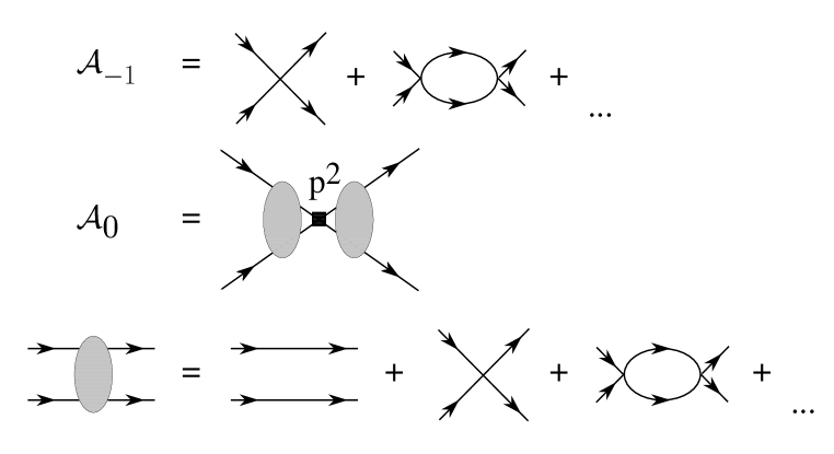
FIG. 2.: Leading and subleading contributions arising from local operators.

Comparing with the expansion of the amplitude eq. (19), these expressions relate the couplings $C_{2n}$ to the low energy scattering data $a$, $r_{n}$:

$$C_{0}(\mu) = {4\pi\over M}\left({1\over-\mu+1/a}\right)\ ,$$ (30)

$$C_{2}(\mu) = {4\pi\over M}\left({1\over-\mu+1/a}\right)^{2}{{r}_{0}\over 2}\ ,$$ (31)

$$C_{4}(\mu) = {4\pi\over M}\left({1\over-\mu+1/a}\right)^{3}\left[{1\over 4}{r}_{0}^{2}+{1\over 2}{{r}_{1}\over\Lambda^{2}}\left({-\mu+1/a}\right)\right]\ .$$ (32)

Note that assuming $r_{n}\sim 1/\Lambda$, these expressions are consistent with the scaling law in eq. (26).

This power counting relies entirely on the behavior of $C_{2n}(\mu)$ as a function of $\mu$ given in eq. (26). The dependence of $C_{2n}(\mu)$ on $\mu$ is determined by the requirement that the amplitude be independent of the arbitrary parameter $\mu$. The physical parameters $a$, $r_{n}$ enter as boundary conditions on the RG equations.

The beta function for each of the couplings $C_{2n}$ is defined by

$$\beta_{2n}\equiv\mu{{\rm d}C_{2n}\over{\rm d}\mu}\ ,$$ (33)

and they can be computed by requiring that any physical quantity (e.g. the scattering amplitude) be independent of $\mu$. In the PDS scheme, the $\mu$ dependence of the $C_{2n}$ coefficients enters either logarithmically or linearly, associated with simple $1/(D-4)$ or $1/(D-3)$ poles respectively. The functions $\beta_{2n}$ follow straightforwardly from $\mu{d\over d\mu}(1/{\cal A})=0$, using the expression for ${\cal A}$ in eq. (25). This gives

$$\beta_{2n}={M\mu\over 4\pi}\sum_{m=0}^{n}C_{2m}C_{2(n-m)}\ .$$ (34)

FIG. 3.: Graphs contributing to the $\beta$-functions for $C_{2n}$

These $\beta$-functions can also be computed from the one-loop diagrams shown in Fig. 3.

We examine the RG equations for the first two couplings, $C_{0}$ and $C_{2}$, in order to explicitly show how one recovers the results in eq. (32) from solving the renormalization group equations. From eq. (34) it follows that

$$\beta_{0} = {M\mu\over 4\pi}C_{0}^{2}\ ,$$ (35)

$$\beta_{2} = 2{M\mu\over 4\pi}C_{0}C_{2}\ .$$ (36)

Integrating these equations relates the $C_{2n}$ coefficients at two different renormalization scales $\mu$ and $\mu_{0}$. Comparing the theory with ${\cal A}$ and its derivatives at $\mu=p=0$ determines the initial values $C_{2n}(0)$ as in eq. (17). The solution for $C_{0}(\mu)$ is

$$C_{0}(\mu)={C_{0}(\mu_{0})\over 1+C_{0}(\mu_{0})M(\mu_{0}-\mu)/4\pi}\ \ \ .$$ (37)

With the boundary condition at $\mu_{0}=0$ provided by eq. (17), $C_{0}(0)=4\pi a/M$, we arrive at the result derived previously for $C_{0}(\mu)$ in eq. (32):

$$C_{0}(\mu)={4\pi\over M}\left({1\over-\mu+1/a}\right)\ .$$ (38)

The RG equation for $C_{2}$ yields

$$C_{2}(\mu)=C_{2}(\mu_{0})\left({C_{0}(\mu)\over C_{0}(\mu_{0})}\right)^{2}\ ,$$ (39)

which when combined with the value of $C_{0}(0)$ and the boundary condition, $C_{2}(0)=C_{0}(0)ar_{0}/2$, from eq. (17), yields for $C_{2}(\mu)$

$$C_{2}(\mu)={4\pi\over M}\left({1\over-\mu+1/a}\right)^{2}{{r}_{0}\over 2}\ ,$$ (40)

as we found previously in eq. (32).

It is possible to solve the complete, coupled RG equation

$$\mu{{\rm d}\ \over{\rm d}\mu}C_{2n}={M\mu\over 4\pi}\sum_{m=0}^{n}C_{2m}C_{2(n-m)}$$ (41)

for the leading small $\mu$ behavior of each of the coefficients $C_{2n}$ . The solution, for $n>0$ is

$$C_{2n}(\mu)={4\pi\over M(-\mu+1/a)}\left({r_{0}/2\over-\mu+1/a}\right)^{n}+O(\mu^{-n})\ .$$ (42)

First note that the scaling property in eq. (26) is realized: $C_{2n}(\mu)\propto\mu^{-(n+1)}$ for $\mu\gg|1/a|$. What is curious is that this leading behavior does not entail a new integration constant for each $n$, but only depends on the two parameters $a$ and $r_{0}$ encountered when solving for $C_{0}(\mu)$ and $C_{2}(\mu)$; this is due to a quasi-fixed point behavior of the RG equations — the $C_{2n}$ couplings are being driven primarily by lower dimensional interactions. One can see this explicitly in our formula eq. (32) for $C_{4}$, where the leading $O(\mu^{-3})$ part of $C_{4}$ depends only on $r_{0}$, while the subleading $O(\mu^{-2})$ part is proportional to $r_{1}$.

This behavior allows us to establish a connection between the present work, and the method of introducing an $s$-channel dibaryon discussed in ref. [8]. The leading $\mu$ behavior of all of the $C_{2n}$ coefficients is determined by the effective range $r_{0}$. If one resums this leading behavior at the $\tilde{N}\tilde{N}$ vertex one finds (for $\mu\sim p\gg 1/|a|$)

$$\sum_{n=0}^{\infty}C_{2n}(\mu)p^{2n} = {4\pi\over M}{1\over-\mu+1/a-{r_{0}p^{2}\over 2}}+O(p^{2})$$ (43)

$$= -{(8\pi/M^{2}r_{0})\over E-(-\mu+1/a)/Mr_{0}}\ .$$ (44)

This looks like an $s$-channel propagator for a particle at rest of mass $[2M+(-\mu+1/a)/Mr_{0}]$, and in fact, for $\mu=0$, corresponds exactly to the dibaryon proposed in [8] to reproduce the scattering due to a short range potential. We see that using the dibaryon is as good as (but no better than) carrying out the effective field theory calculation to $O(p^{1})$. The subleading corrections can be accounted for by including the subleading part of the $C_{4}(\mu)p^{4}$ vertex proportional to $r_{1}$, and which occurs at $O(p^{2})$. This dibaryon was recently used with great success in the three-body problem [16].

C Luke-Manohar velocity scaling

In ref. [12] a rescaling of fields was shown to eliminate the heavy mass scale $M$ from the Lagrangian, and allow a simple power counting in terms of the velocity $v$ of the interacting nucleons. One finds that a four fermion operator scales as $v$, and is therefore irrelevant as $v\to 0$. It is instructive to see why this conclusion is avoided in the theory with large scattering length, where the interaction has a large effect on scattering at the low momentum $p\sim 1/|a|$.

The rescaled theory is described in terms of dimensionless energy and momentum variables, ${\cal E}=E/Mv^{2}$ and ${\cal P}=p/Mv$, corresponding to a rescaling of the spacetime coordinates $T=tMv^{2}$, $X=xMv$. The nucleon fields are rescaled as $\Psi=\tilde{N}/(Mv)^{3/2}$, in order to give a canonical energy term. Performing the Luke-Manohar scaling on our toy theory in a naive manner yields the action

$$S=\int d^{3}XdT\ \ {\Psi^{\dagger}}\left(i\partial_{T}+{1\over 2}\nabla^{2}_{X}\right)\Psi+C_{0}M^{2}v({\Psi^{\dagger}}\Psi)^{2}+...$$ (45)

This demonstrates the familiar result that a contact interaction ($\delta$-function potential) is an irrelevant operator in nonrelativistic scattering in $D=4$ dimensions, since the interaction vanishes as $v\to 0$. This is certainly true when the underlying theory is perturbative, but it fails when it is strongly coupled and there is a large scattering length. In that case we should be using the running coupling constants discussed in the previous section, keeping in mind that the renormalization scale $\mu$ must also be rescaled as $\hat{\mu}=\mu/Mv$, since it is treated on the same footing as momenta. Replacing $C_{0}$ in the above expression with the value of the running coupling $C_{0}(\mu)$ from eq. (38) we find the rescaled interaction

$$\int d^{3}XdT\ {4\pi Mv\over-\hat{\mu}Mv+1/a}({\Psi^{\dagger}}\Psi)^{2}+...$$ (46)

where $\hat{\mu}\sim 1$. Now it is evident once again that the limit $a\to\infty$ corresponds to tuning $C_{0}$ to a UV fixed point. Near that fixed point, the four fermion interaction is a relevant operator (it doesn’t decrease as $v$ gets smaller), which is why it has a large effect on scattering at low velocity. Only for the very low velocities $v\ \raise 1.29167pt\hbox{$<$\kern-7.5pt\lower 4.30554pt\hbox{$\sim$}}\ 1/Ma$ does it become irrelevant, at which point perturbation theory is once again justified.

III The effective field theory expansion for realistic NN scattering

We now turn to the problem of interest, realistic low momentum nucleon-nucleon scattering. The goal of an effective field theory treatment is to provide a systematic expansion for computing $NN$ phase shifts at low momenta, which means that the phenomenology of the two nucleon system can be approximated to any desired accuracy. While an effective field theory treatment will never in practice compete with the extremely precise phenomenological potential model descriptions of the $NN$ phase shifts, it will provide a framework to compute relativistic effects and inelastic processes, as well as to reliably estimate errors at any order in the expansion. Furthermore, as it is a perturbative expansion, the effective field theory approach will hopefully be useful for many-body systems for which potential models are computationally intractable.

Realistic $NN$ scattering is more complicated than our toy model for several reasons: the inclusion of explicit pion fields, the spin and isospin degrees of freedom, and the need to include relativistic corrections in the power counting scheme. Nevertheless, we will show that the momentum expansion for this theory closely follows the discussion in §II B, and that for $p\ \raise 1.29167pt\hbox{$<$\kern-7.5pt\lower 4.30554pt\hbox{$\sim$}}\ m_{\pi}$ the expansion improves as the pion mass gets smaller. This is an important result, as it means that there is a region of QCD parameters for which our results hold with high accuracy. (We do not, however, take the pion mass so small that $am_{\pi}$ is also small.)

Since we are performing a momentum expansion, it is important to understand the scale at which it fails. In the 1-nucleon sector, the expansion is in powers of $(m_{\pi}/\Lambda_{\chi})$ and $(p/\Lambda_{\chi})$, where $\Lambda_{\chi}=4\pi f=1.6{\rm GeV}$, ($f=132\ {\rm\ MeV}$ being the pion decay constant). However, we find that the chiral expansion for $NN$ scattering entails the new scale,

$$\Lambda_{NN}\equiv{8\pi f^{2}\over g_{A}^{2}M}=300\,{\rm\ MeV}\ .$$ (47)

It is disturbing that $\eta_{\pi}\equiv(m_{\pi}/\Lambda_{NN})=0.46$, suggesting that our expansion will not converge rapidly. However, if one looks at the Yukawa piece of the one pion exchange (OPE) potential in the ${}^{1}\kern-1.4ptS_{0}$ channel, it only binds nucleons for $\eta_{\pi}\geq 1.7$, while for the true value $\eta_{\pi}=.46$, the $NN$ phase shift from the OPE Yukawa potential never gets larger than $\sim.25$ radians. Thus there is empirical evidence that the chiral expansion parameter for $NN$ scattering is about $30\%$, and it is reasonable that for momenta $p\sim m_{\pi}$ the expansion will converge fairly quickly.

A The chiral expansion

We need to consider a theory of nucleons interacting with pions and with themselves through contact interactions consistent with chiral symmetry. Nucleons are described by isodoublet fields $N$, while the pions are described by the field

$$\xi(x)=e^{i\Pi/f}\ ,\qquad\Pi=\left(\matrix{{\pi^{0}\over\sqrt{2}}&\pi^{+}\cr\pi^{-}&-{\pi^{0}\over\sqrt{2}}\cr}\right)$$ (48)

and $f$ is the pion decay constant normalized to be

$$f=132\ {\rm\ MeV}\ .$$ (49)

Under $SU(2)_{L}\times SU(2)_{R}$ chiral symmetry the fields transform as

$$\xi\to L\xi U^{\dagger}=U\xi R^{\dagger}\ ,\qquad\Sigma\equiv\xi^{2}\to L\Sigma R^{\dagger}\ ,\qquad N\to UN\ ,$$ (50)

where $L$, $R$ are constant $SU(2)$ matrices and $U(x)$ is a pion-dependent $SU(2)$ matrix. The vector and axial-vector pion currents are given by

$$V_{\mu}={1\over 2}(\xi\partial_{\mu}\xi^{\dagger}+\xi^{\dagger}\partial_{\mu}\xi)\ ,\qquad A_{\mu}={i\over 2}(\xi\partial_{\mu}\xi^{\dagger}-\xi^{\dagger}\partial_{\mu}\xi)$$ (51)

where the axial current $A_{\mu}$ and the chiral covariant derivative $D_{\mu}=(\partial_{\mu}+V_{\mu})$ transform linearly as

$$A_{\mu}\to UA_{\mu}U^{\dagger}\ ,\qquad D_{\mu}\to UD_{\mu}U^{\dagger}\ .$$ (52)

In the 1-nucleon sector, the chiral Lagrangian is then given by

$${\cal L}=N^{\dagger}(iD_{0}+\vec{D}^{2}/2M)N+{f^{2}\over 8}{\rm Tr\,}\partial_{\mu}\Sigma^{\dagger}\partial^{\mu}\Sigma+{f^{2}\over 4}\omega{\rm Tr\,}M_{q}(\Sigma+\Sigma^{\dagger})+g_{A}N^{\dagger}\vec{A}\cdot\vec{\sigma}N+\dots$$ (53)

where $M_{q}$ is the quark mass matrix diag$(m_{u},m_{d})$, $\omega$ has dimensions of mass with $m_{\pi}^{2}=\omega(m_{u}+m_{d})$, and the ellipses refers to all additional operators.

When considering the 2-nucleon sector, one must include local four nucleon operators in the effective lagrangian. Due to spin and isospin degrees of freedom, the number of four fermion operators grows rapidly with the number of derivatives. To the order we will be working, we need only consider operators without pion fields and with $\leq 2$ derivatives, or no derivatives and one insertion of the quark mass matrix. Rather than writing down the operators in the chiral Lagrangian, it is simplest to identify their matrix elements between particular partial waves. With no derivatives, these contact interactions only effect $S$-waves. Thus there are two independent $C_{0}$ operators associated with the ${}^{1}\kern-1.4ptS_{0}$ and ${}^{3}\kern-1.4ptS_{1}$ channels [3]. Denoting the partial waves as

$$|\alpha\rangle=|SLJm,E\rangle$$ (54)

we normalize the two $C_{0}^{(\gamma)}$ operators by defining the Born amplitude for ${\cal L}_{C_{0}}$, the four fermion interactions involving no derivatives, as

$$\langle\alpha|{\cal L}_{C_{0}}|\beta\rangle=-\left({Mp\over 2\pi}\right)\sum_{\gamma}C_{0}^{(\gamma)}\delta_{\alpha\gamma}\delta_{\beta\gamma}\ ,\qquad\gamma=\{{}^{1}\kern-1.4ptS_{0},{}^{3}\kern-1.4ptS_{1}\}\ .$$ (55)

There are seven independent two derivative contact interactions [4]. These operators change orbital angular momentum by $\Delta L=0$ or $\Delta L=2$. Therefore, in analogy to eq. (55), we can define seven $C_{2}^{(\gamma)}$ couplings by

$$\langle\alpha|{\cal L}_{C_{2}}|\beta\rangle = -\left({Mp\over 2\pi}\right)p^{2}\left[\sum_{\gamma}C_{2}^{(\gamma)}\delta_{\alpha\gamma}\delta_{\beta\gamma}+(C_{2}^{({}^{3}\kern-0.98ptS_{1}-{}^{3}\kern-0.98ptD_{1})}\delta_{\alpha,{}^{3}\kern-0.98ptS_{1}}\delta_{\beta,{}^{3}\kern-0.98ptD_{1}}+\alpha\leftrightarrow\beta)\right]\ ,$$ (56)

$$\gamma = \{{}^{1}\kern-1.4ptS_{0},{}^{1}\kern-1.4ptP_{1},{}^{3}\kern-1.4ptS_{1},{}^{3}\kern-1.4ptP_{0},{}^{3}\kern-1.4ptP_{1},{}^{3}\kern-1.4ptP_{2}\}\ .$$ (57)

As before, $p^{2}\equiv ME$.

At the same order as the $C_{2}$ operators are four fermion operators with a single insertion of the quark mass matrix $M_{q}$. If we ignore isospin violation, then $M_{q}\propto m_{\pi}^{2}$ times a unit matrix in isospin space, and so these operators have the same structure as the $C_{0}^{(\gamma)}$ operators. We parametrize them as

$$\langle\alpha|{\cal L}_{D_{2}}|\beta\rangle=-\left({Mp\over 2\pi}\right)m_{\pi}^{2}\sum_{\gamma}D_{2}^{(\gamma)}\delta_{\alpha\gamma}\delta_{\beta\gamma}\ ,\qquad\gamma=\{{}^{1}\kern-1.4ptS_{0},{}^{3}\kern-1.4ptS_{1}\}\ .$$ (58)

Since the ${}^{1}\kern-1.4ptS_{0}$ and ${}^{3}\kern-1.4ptS_{1}$ scattering lengths are large compared with $1/m_{\pi}$, the power counting in these channels is the same as for the example of §2: for $\mu\sim m_{\pi}$, $C_{0}^{(\gamma)}(\mu)\propto 1/\mu$, $C_{2}^{(\gamma)}(\mu)\propto 1/\mu^{2}$ and $D_{2}^{(\gamma)}(\mu)\propto 1/\mu^{2}$ for $\gamma=\{{}^{1}\kern-1.4ptS_{0},{}^{3}\kern-1.4ptS_{1}\}$. A single exchange of a potential pion contributes to the amplitude a factor of

$$i{g_{A}^{2}\over 2f^{2}}{{\bf q}\cdot\sigma^{1}{\bf q}\cdot\sigma^{2}\over{\bf q}^{2}+m_{\pi}^{2}}\tau^{1}\cdot\tau^{2}$$ (59)

which scales as $O(1)$ in the chiral expansion. Thus one pion exchange occurs at the same order as an insertion of $C_{2}p^{2}$ or $D_{2}m_{\pi}^{2}$ in the ${}^{1}\kern-1.4ptS_{0}$ and ${}^{3}\kern-1.4ptS_{1}$ channels, and pion exchange may be treated perturbatively. A new feature of the theory with pions is that this scaling behavior breaks down not only at low momentum, $p\sim 1/|a|$, but also at sufficiently high momentum. This can be seen by examining the RG equations for $C_{0}^{(\gamma)}$.

FIG. 4.: Leading contributions to the $\beta$-functions for $C_{0}^{\gamma}$, including pions

The exact beta function for the $C_{0}^{(\gamma)}$ coefficients comes from the graphs of Fig. 4, and one finds

$$\beta_{0}^{({}^{1}\kern-0.98ptS_{0})}=\mu{{\rm d}C_{0}^{({}^{1}\kern-0.98ptS_{0})}\over{\rm d}\mu\ \ }={M\mu\over 4\pi}\left\{\left(C_{0}^{({}^{1}\kern-0.98ptS_{0})}\right)^{2}+2C_{0}^{({}^{1}\kern-0.98ptS_{0})}{g_{A}^{2}\over 2f^{2}}+\left({g_{A}^{2}\over 2f^{2}}\right)^{2}\right\},$$ (60)

$$\beta_{0}^{({}^{3}\kern-0.98ptS_{1})}=\mu{{\rm d}C_{0}^{({}^{3}\kern-0.98ptS_{1})}\over{\rm d}\mu\ \ }={M\mu\over 4\pi}\left\{\left(C_{0}^{({}^{3}\kern-0.98ptS_{1})}\right)^{2}+2C_{0}^{({}^{3}\kern-0.98ptS_{1})}{g_{A}^{2}\over 2f^{2}}+9\left({g_{A}^{2}\over 2f^{2}}\right)^{2}\right\}.$$ (61)

Solving the RG equation for the singlet channel eq. (60) with the boundary condition $C_{0}^{({}^{1}\kern-0.98ptS_{0})}(0)=4\pi a_{1}/M$, where $a_{1}$ is the ${}^{1}\kern-1.4ptS_{0}$ scattering length, we find

$$C_{0}^{({}^{1}\kern-0.98ptS_{0})}(\mu)=-{4\pi\over M\mu}\left({1\over 1-{1\over\mu(a_{1}+1/\Lambda_{NN})}}+{\mu\over\Lambda_{NN}}\right),$$ (62)

where $\Lambda_{NN}$ is given in eq. (47). Since $\Lambda_{NN}\gg 1/|a_{1}|$, for $\mu\gg 1/|a_{1}|$ we have

$$C_{0}^{({}^{1}\kern-0.98ptS_{0})}(\mu)\simeq-{4\pi\over M\mu}\left(1+{\mu\over\Lambda_{NN}}\right)\ ,$$ (63)

and so the power counting changes for $\mu\ \raise 1.29167pt\hbox{$>$\kern-7.5pt\lower 4.30554pt\hbox{$\sim$}}\ \Lambda_{NN}$; in fact the UV fixed point toward which $C_{0}^{({}^{1}\kern-0.98ptS_{0})}$ is driven largely cancels the $\delta$-function component of the single pion exchange in the ${}^{1}\kern-1.4ptS_{0}$ channel. Similarly, power counting is found to change at $\mu\sim\Lambda_{NN}$ in the ${}^{3}\kern-1.4ptS_{1}$ channel as well. As a result, the power counting developed in §2, with one pion exchange treated as $O(1)$, works only up to $p\sim\Lambda_{NN}$. At that point one pion exchange and a $C_{0}$ insertion become equally important. The power counting that we follow in this paper is therefore expected to fail completely at momenta on the order of $\Lambda_{NN}$.

Up to now we have only discussed the scaling of the $C_{2}$ interactions in the ${}^{1}\kern-1.4ptS_{0}$ and ${}^{3}\kern-1.4ptS_{1}$ channels. The $1/\mu^{2}$ scaling of these couplings is due to multiplicative renormalization by $C_{0}$. Such renormalization does not occur for $C_{2}$ in any of the $P$-wave channels, and so these couplings will be $O(p^{0})$. Thus the leading contribution to the $P$-wave (and all higher partial wave) amplitudes occurs at $O(1)$ and is simply a single pion exchange (the Born approximation OPE). It is well-known that this accounts very well for the observed phase shifts. The subleading contribution to the $P$-wave amplitude is due to the exchange of two potential pions at $O(p^{1})$, while the $C_{2}p^{2}$ operators enter at $O(p^{2})$, along with the two-loop graph with the exchange of three pions.

The transition operator coefficient, $C_{2}^{({}^{3}\kern-0.98ptS_{1}-{}^{3}\kern-0.98ptD_{1})}$ is different from the others as it is multiplicatively renormalized by $C_{0}^{({}^{3}\kern-0.98ptS_{1})}$, but its beta function is half as big as that for $C_{2}^{({}^{3}\kern-0.98ptS_{1})}$. For small $\mu$, $C_{2}^{({}^{3}\kern-0.98ptS_{1}-{}^{3}\kern-0.98ptD_{1})}(\mu)\sim 1/\mu$, and it enters the calculation at $O(p^{1})$. An important aspect of the $O(p^{1})$ calculation of the ${}^{1}\kern-1.4ptS_{0}$ and ${}^{3}\kern-1.4ptS_{1}$ scattering amplitudes is the absence of new undetermined coefficients $C_{4}^{({}^{1}\kern-0.98ptS_{0})}$ and $C_{4}^{({}^{3}\kern-0.98ptS_{1})}$. The renormalization group scaling determines the leading behavior of these couplings. For small $\mu$ (but $|a|\mu\gg 1$), $C_{4}^{(\gamma)}(\mu)=-(M\mu/4\pi)C_{2}^{(\gamma)}(\mu)^{2}$.

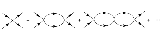
FIG. 5.: Graphs contributing to the leading amplitude ${\cal A}_{-1}$.

It is now possible to perform a systematic chiral expansion for $NN$ scattering amplitudes in the situation where $m_{\pi}$ is small, (but $|a|m_{\pi}$ is not). Denoting our expansion parameter by $Q$, representing equally $p$ or $m_{\pi}$, and taking $\mu\sim Q$ the leading amplitude is $O(Q^{-1})$ and is simply the bubble sum of $C_{0}^{(\gamma)}$ interactions, shown in Fig. 5. The subleading contribution is $O(Q^{0})$, and involves an insertion of either a single pion exchange, a $C_{2}$ operator, or a $D_{2}$ operator, dressed to all orders by the $C_{0}$ interaction, as shown in Fig. 6. At $O(Q^{1})$ one finds both two pion exchange (involving both the two pion vertex as well as iterated one OPE), four derivative operators, and so forth. It may be tempting to sum up the OPE potential exactly as is typically done (e.g., ref. [3]), but it is not consistent to do so while leaving out the arbitrarily higher derivative contact interactions that are required to renormalize the pion ladders. By neglecting these higher derivative terms one is making a model for the short distance physics, and the result one gets is not any more accurate for having included the multiple pion exchange.

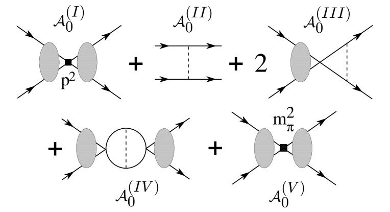
FIG. 6.: Graphs contributing to the subleading amplitude ${\cal A}_{0}$; the shaded ovals are defined in Fig. 2.

B The ${}^{1}\kern-1.4ptS_{0}$ channel to subleading order

In the isotriplet ${}^{1}\kern-1.4ptS_{0}$ channel the nucleons are exclusively in an $S=L=J=0$ state. The leading $O(Q^{-1})$ contribution to scattering in this channel is from the bubble chain of $C^{({}^{1}\kern-0.98ptS_{0})}_{0}$ operators, as shown in Fig. 5

$${\cal A}_{-1}=-{C^{({}^{1}\kern-0.98ptS_{0})}_{0}\over 1+C^{({}^{1}\kern-0.98ptS_{0})}_{0}{M\over 4\pi}\left(\mu+ip\right)}\ .$$ (64)

Since we are computing the amplitude between plane wave states, we omit from ${\cal A}$ the normalization factor $(Mp/2\pi)$ appearing in eqs. (55-58). There is only one unknown parameter that needs to be fit to data and for simplicity we will require that the amplitude at this order reproduce the ${}^{1}\kern-1.4ptS_{0}$ ($np$) scattering length $a_{1}=-23.714\pm 0.013\ {\rm fm}$. This determines $C_{0}^{({}^{1}\kern-0.98ptS_{0})}(m_{\pi})=-3.51{\rm\ fm}^{2}$, where we have chosen to renormalize at $\mu=m_{\pi}$ and the behavior of the phase shift over a range of momenta resulting from this fit is shown in Fig. 7.

At next order $Q^{0}$ there are contributions from insertions of higher dimension local operators and also from potential pion exchange. The $O(Q^{0})$ contribution to the amplitude is written as a sum of the five terms, ${\cal A}_{0}={\cal A}_{0}^{(I)}+{\cal A}_{0}^{(II)}+{\cal A}_{0}^{(II)}+{\cal A}_{0}^{(IV)}+{\cal A}_{0}^{(V)}$. The local operators at this order involve either two spatial derivatives, $C_{2}^{({}^{1}\kern-0.98ptS_{0})}$, or one insertion of the light quark mass matrix, $D_{2}^{({}^{1}\kern-0.98ptS_{0})}$. Expressions for the graphs shown in Fig. 6 which we presented in ref. [2] are

$${\cal A}_{0}^{(I)} = -C_{2}^{({}^{1}\kern-0.98ptS_{0})}p^{2}\left[{{\cal A}_{-1}\over C_{0}^{({}^{1}\kern-0.98ptS_{0})}}\right]^{2}\ \ \ ,$$ (65)

$${\cal A}_{0}^{(II)} = \left({g_{A}^{2}\over 2f^{2}}\right)\left(-1+{m_{\pi}^{2}\over 4p^{2}}\ln\left(1+{4p^{2}\over m_{\pi}^{2}}\right)\right)\ ,$$ (66)

$${\cal A}_{0}^{(III)} = {g_{A}^{2}\over f^{2}}\left({m_{\pi}M{\cal A}_{-1}\over 4\pi}\right)\Bigg{(}-{(\mu+ip)\over m_{\pi}}+{m_{\pi}\over 2p}\left[\tan^{-1}\left({2p\over m_{\pi}}\right)+{i\over 2}\ln\left(1+{4p^{2}\over m_{\pi}^{2}}\right)\right]\Bigg{)}\ ,$$ (67)

$${\cal A}_{0}^{(IV)} = {g_{A}^{2}\over 2f^{2}}\left({m_{\pi}M{\cal A}_{-1}\over 4\pi}\right)^{2}\Bigg{(}-\left({\mu+ip\over m_{\pi}}\right)^{2}+\left[i\tan^{-1}\left({2p\over m_{\pi}}\right)-{1\over 2}\ln\left({m_{\pi}^{2}+4p^{2}\over\mu^{2}}\right)+1\right]\Bigg{)}\ ,$$ (68)

$${\cal A}_{0}^{(V)} = -D^{({}^{1}\kern-0.98ptS_{0})}_{2}m_{\pi}^{2}\left[{{\cal A}_{-1}\over C_{0}^{({}^{1}\kern-0.98ptS_{0})}}\right]^{2}\ .$$ (69)

The two-loop diagram in ${\cal A}_{0}^{(IV)}$ involving the exchange of a potential pion between two contact terms is divergent in both three and four dimensions. In the PDS scheme we subtract the poles in three and four dimensions leaving this graph logarithmically as well as power-law dependent on the renormalization point $\mu$. As the coefficient of the four-dimensional divergence is proportional to the mass of the pion squared, the required isospin conserving counterterm with coefficient $D^{({}^{1}\kern-0.98ptS_{0})}_{2}(\mu)$ depends on the sum of the light quark masses, $m_{u}+m_{d}$ and gives rise to ${\cal A}_{0}^{(V)}$. In addition, for convenience we have absorbed some of the $\mu$-independent terms from ${\cal A}_{0}^{(IV)}$ into the definition of $D^{({}^{1}\kern-0.98ptS_{0})}_{2}(\mu)$. At this order there are three unknown counterterms that need to be fit to data, $C_{0}^{({}^{1}\kern-0.98ptS_{0})}(\mu),C_{2}^{({}^{1}\kern-0.98ptS_{0})}(\mu)$ and $D^{({}^{1}\kern-0.98ptS_{0})}_{2}(\mu)$. As the amplitude can be written as a function of $C_{0}^{({}^{1}\kern-0.98ptS_{0})}(\mu)+m_{\pi}^{2}D^{({}^{1}\kern-0.98ptS_{0})}_{2}(\mu)$, the dependence of observables upon $C_{0}^{({}^{1}\kern-0.98ptS_{0})}(\mu)$ and $D^{({}^{1}\kern-0.98ptS_{0})}_{2}(\mu)$ individually is an artifact of the perturbative expansion, and is indicative of the size of higher order effects. Conventionally, the scattering data in the $NN$ sector is presented in terms of phase shifts. In this channel, the phase shift is simply related to the amplitude ${\cal A}$ by

$$S=e^{2i\delta}=1+i{Mp\over 2\pi}{\cal A}\ \ \ ,$$ (70)

leading to

$$\delta = {1\over 2i}\ln\left(1+i{Mp\over 2\pi}{\cal A}\right)\ .$$ (71)

Expanding both sides to a given order in $Q$ with $\delta=\left(\delta^{(0)}+\delta^{(1)}+\ldots\right)$ gives

$$\delta^{(0)} = {1\over 2i}\ln\left(1+i{Mp\over 2\pi}{\cal A}_{-1}\right)\ ,\qquad\delta^{(1)}={Mp\over 4\pi}\left({{\cal A}_{0}\over 1+i{Mp\over 2\pi}{\cal A}_{-1}}\right)\ .$$ (72)

Here superscripts denote the order in Q. Our expression for the amplitude ${\cal A}$ gives an $S$-matrix that is unitary up to the order we have computed, i.e. if the amplitude is computed up to $O(Q^{k})$, then $S^{\dagger}S=1+O(Q^{k+2})$.

It is convenient to choose $\mu=m_{\pi}$. Expressions for the scattering length and effective range are determined from the expansion, $p\cot\delta=ip+4\pi/M{\cal A}_{-1}-4\pi{\cal A}_{0}/M{\cal A}_{-1}^{2}$, which yields to the order we are working,

$${1\over a_{1}}=\left(m_{\pi}+{4\pi\over MC_{0}^{({}^{1}\kern-0.98ptS_{0})}(m_{\pi})}\right)-{4\pi D_{2}^{({}^{1}\kern-0.98ptS_{0})}(m_{\pi})m_{\pi}^{2}\over M(C_{0}^{({}^{1}\kern-0.98ptS_{0})}(m_{\pi}))^{2}}\ \ \ ,$$ (73)

and

$$r_{0}={8\pi C_{2}^{({}^{1}\kern-0.98ptS_{0})}(m_{\pi})\over M(C_{0}^{({}^{1}\kern-0.98ptS_{0})}(m_{\pi}))^{2}}+{g_{A}^{2}M\over 12\pi f^{2}}\left(1+{16\pi\over C_{0}^{({}^{1}\kern-0.98ptS_{0})}(m_{\pi})m_{\pi}M}+{96{\pi}^{2}\over(C_{0}^{({}^{1}\kern-0.98ptS_{0})}(m_{\pi})m_{\pi}M)^{2}}\right).$$ (74)

The choice

$$C_{0}(m_{\pi})=-3.63~{}{\rm fm}^{2}\ ,\qquad D_{2}(m_{\pi})\equiv 0\ ,\qquad C_{2}(m_{\pi})=2.92~{}{\rm fm}^{4}\ ,$$ (75)

is consistent with the experimental values of the scattering length and effective range . About $43\%$ of the effective range is due to $C_{2}(m_{\pi})$. The phase shift resulting from these parameters is shown in Fig. 7.

Alternatively, we consider fitting the phase shift from the Nijmegen partial wave analysis [32] over the momentum range $p\leq 200{\rm\ MeV}$, treating $C_{0}^{({}^{1}\kern-0.98ptS_{0})}$, $D_{2}^{({}^{1}\kern-0.98ptS_{0})}$ and $C_{2}^{({}^{1}\kern-0.98ptS_{0})}$ as free parameters. The results are

$$C_{0}^{({}^{1}\kern-0.98ptS_{0})}(m_{\pi})=-3.34{\rm\ fm}^{2}\ ,\qquad D_{2}^{({}^{1}\kern-0.98ptS_{0})}(m_{\pi})=-0.42{\rm\ fm}^{4}\ ,\qquad C_{2}^{({}^{1}\kern-0.98ptS_{0})}(m_{\pi})=3.24{\rm\ fm}^{4}\ \ \ ,$$ (76)

which give the phase shift plotted in Fig. 7. As is apparent from Fig. 7, the agreement of the phase shift with data is excellent at quite large values of $p$. Furthermore, the coupling $C_{0}^{({}^{1}\kern-0.98ptS_{0})}(m_{\pi})$ is close to its leading order value (in the limit of large scattering length), $-(4\pi/Mm_{\pi})=-3.7{\rm\ fm}^{2}$, and $C_{2}^{({}^{1}\kern-0.98ptS_{0})}(m_{\pi})$ is also near its expected size, suggesting that our expansion is valid in this channel. However, for $p>100{\rm\ MeV}$ the magnitude of the ratio ${\cal A}_{0}/{\cal A}_{-1}$ is greater than $\sim 0.5$ and it is difficult to justify the approximations we have made, e.g. neglecting terms suppressed by $({\cal A}_{0}/{\cal A}_{-1})^{2}$. The difference between the two fitting procedures is attributable to effects higher order in our expansion.

FIG. 7.: The phase shift $\delta$ for the ${}^{1}\kern-1.4ptS_{0}$ channel. The dot-dashed curve is the one parameter fit at $O(Q^{-1})$, that reproduces the scattering length. The dotted and dashed curves are the fits at $O(Q^{0})$ in eqs. (75, 76) respectively. The dashed curve corresponds to fitting $\delta$ between $0<p<200\ {\rm MeV}$, while the dotted curve corresponds to fitting the scattering length and effective range. The solid line shows the results of the Nijmegen partial wave analysis.

C The ${}^{3}S_{1}-{}^{3}D_{1}$ channels to subleading order

The analysis of the isosinglet ${}^{3}\kern-1.4ptS_{1}-{}^{3}\kern-1.4ptD_{1}$ channel is richer than the ${}^{1}\kern-1.4ptS_{0}$ channel since there are two different orbital angular momentum states involved. The power counting in the ${}^{3}\kern-1.4ptS_{1}$ channel is the same as for the ${}^{1}\kern-1.4ptS_{0}$ channel. However, we must also consider how the coefficients of the operators contributing to scattering in the ${}^{3}\kern-1.4ptD_{1}$ channel and the coefficients of the operators that give rise to ${}^{3}\kern-1.4ptS_{1}-{}^{3}\kern-1.4ptD_{1}$ mixing behave under renormalization group scaling and at what order in the $Q$ expansion they contribute to observables. Firstly, operators between two ${}^{3}\kern-1.4ptD_{1}$ states are not renormalized by the leading operators, which project out only ${}^{3}\kern-1.4ptS_{1}$ states. Further, they involve a total of four spatial derivatives, two on the incoming nucleons, and two on the out-going nucleons. Therefore, such operators contribute at $O(Q^{4})$, and can be safely neglected. Consequently, amplitudes for scattering from an ${}^{3}\kern-1.4ptD_{1}$ state into an ${}^{3}\kern-1.4ptD_{1}$ state are dominated by single potential pion exchange which contributes at $O(Q^{0})$. Single pion exchange describes well this partial wave in the momentum range we are considering. Secondly, operators connecting ${}^{3}\kern-1.4ptD_{1}$ and ${}^{3}\kern-1.4ptS_{1}$ states involve 2 spatial derivatives (acting on the ${}^{3}\kern-1.4ptD_{1}$ state) and are renormalized by the leading operators, but only on the $L=0$ “side” of the operator. Therefore the coefficient of this operator, $C_{2}^{({}^{3}\kern-0.98ptS_{1}-{}^{3}\kern-0.98ptD_{1})}\sim 1/\mu$, and contributes at $O(Q^{1})$. Hence it can also be neglected at the order we are working. Thus, mixing between ${}^{3}\kern-1.4ptD_{1}$ and ${}^{3}\kern-1.4ptS_{1}$ states is dominated by single potential pion exchange dressed by a bubble chain of $C_{0}^{({}^{3}\kern-0.98ptS_{1})}$ operators and a parameter free prediction for this mixing as a function of momentum exists at $O(Q^{0})$.

We denote the amplitude at $O(Q^{n})$ by ${\cal A}_{n[LL^{\prime}]}$, where $L$ and $L^{\prime}$ are the initial and final orbital angular momenta. As in the ${}^{1}\kern-1.4ptS_{0}$ channel, we omit from ${\cal A}$ the normalization factor $(Mp/2\pi)$ appearing in eqs. (55-58) since we are computing the amplitude between plane wave states. At leading $O(Q^{-1})$ in the expansion there is a contribution only to the ${}^{3}\kern-1.4ptS_{1}$ partial wave:

$${\cal A}_{-1[00]}=-{C^{({}^{3}\kern-0.98ptS_{1})}_{0}\over 1+C^{({}^{3}\kern-0.98ptS_{1})}_{0}{M\over 4\pi}\left(\mu+ip\right)}\ ,\qquad{\cal A}_{-1[02]}\ =\ {\cal A}_{-1[20]}\ =\ {\cal A}_{-1[22]}\ =\ 0\ .$$ (77)

At $O(Q^{0})$ there are contributions from graphs of the same form as in the amplitude for ${}^{1}\kern-1.4ptS_{0}$ scattering, shown in Fig. 6. Using the same identification of graphs as in the ${}^{1}\kern-1.4ptS_{0}$ channel, and the similar notation, ${\cal A}_{0[L,L^{\prime}]}={\cal A}_{0[L,L^{\prime}]}^{(I)}+...$,we find that

$${\cal A}_{0[00]}^{(I)}=-C_{2}^{({}^{3}\kern-0.98ptS_{1})}p^{2}\left[{{\cal A}_{-1[00]}\over C_{0}^{({}^{3}\kern-0.98ptS_{1})}}\right]^{2}\ ,\qquad{\cal A}_{0[02]}^{(I)}\ =\ {\cal A}_{0[20]}^{(I)}\ =\ {\cal A}_{0[22]}^{(I)}\ =\ 0\ ,$$ (78)

arising from a single insertion of the local operator involving two spatial derivatives. Single potential pion exchange in the $t$-channel gives

$${\cal A}_{0[00]}^{(II)}\ = \ -{g_{A}^{2}\over 2f^{2}}\left[1-{m_{\pi}^{2}\over 2p^{2}}Q_{0}(z)\right]\ \ \ ,$$ (79)

$${\cal A}_{0[02]}^{(II)}\ = \ {\cal A}_{0[20]}^{(II)}\ =\ -{g_{A}^{2}\over\sqrt{2}f^{2}}\left[Q_{0}(z)+Q_{2}(z)-2Q_{1}(z)\right]\ \ \ ,$$ (80)

$${\cal A}_{0[22]}^{(II)}\ = \ -{g_{A}^{2}m_{\pi}^{2}\over 4f^{2}p^{2}}\left[Q_{2}(z)+{6p^{2}\over 5m_{\pi}^{2}}\left(Q_{1}(z)-Q_{3}(z)\right)\right]\ \ \ ,$$ (81)

where $z=1+m_{\pi}^{2}/(2p^{2})$ and $Q_{k}(z)$ denotes the $k$-th order irregular Legendre function,

$$Q_{0}={1\over 2}\log\left({z+1\over z-1}\right)\ ,\quad Q_{1}=zQ_{0}-1\ ,\quad(n+1)Q_{n+1}=(2n+1)zQ_{n}-nQ_{n-1}\ .$$ (82)

The contribution from single pion exchange across the end of a bubble chain of operators with coefficient $C_{0}^{({}^{3}\kern-0.98ptS_{1})}$ is

$${\cal A}_{0[00]}^{(III)} = {g_{A}^{2}\over f^{2}}\left({m_{\pi}M{\cal A}_{-1[00]}\over 4\pi}\right)\ \Bigg{(}-{(\mu+ip)\over m_{\pi}}+{m_{\pi}\over 2p}\left[\tan^{-1}\left({2p\over m_{\pi}}\right)+{i\over 2}\ln\left(1+{4p^{2}\over m_{\pi}^{2}}\right)\right]\Bigg{)}\ \ \ ,$$ (83)

$${\cal A}_{0[02]}^{(III)}\ = \ {\cal A}_{0[20]}^{(III)}$$ (84)

$$= {g_{A}^{2}\over\sqrt{2}f^{2}}\left({M{\cal A}_{-1[00]}\over 4\pi}\right)p^{2}\left[-{3m_{\pi}^{3}\over 4p^{4}}+{m_{\pi}^{2}\over 8p^{5}}(3m_{\pi}^{2}+4p^{2})\tan^{-1}\left({2p\over m_{\pi}}\right)\right.$$ (86)

$$\left.\qquad\qquad+i\left(-{3m_{\pi}^{2}\over 4p^{3}}+{1\over 2p}+{m_{\pi}^{2}\over 4p^{3}}\left(1+{3m_{\pi}^{2}\over 4p^{2}}\right)\log\left(1+{4p^{2}\over m_{\pi}^{2}}\right)\right)\right]\ \ \ ,$$

$${\cal A}_{0[22]}^{(III)}\ = \ 0\ ,$$ (87)

while

$${\cal A}_{0[00]}^{(IV)} = {g_{A}^{2}\over 2f^{2}}\left({m_{\pi}M{\cal A}_{-1[00]}\over 4\pi}\right)^{2}\Bigg{(}-\left({\mu+ip\over m_{\pi}}\right)^{2}+i\tan^{-1}\left({2p\over m_{\pi}}\right)-{1\over 2}\ln\left({m_{\pi}^{2}+4p^{2}\over\mu^{2}}\right)+1\Bigg{)}\ ,$$ (88)

$${\cal A}_{0[02]}^{(IV)}\ = \ {\cal A}_{0[20]}^{(IV)}\ =\ {\cal A}_{0[22]}^{(IV)}\ =\ 0\ ,$$ (89)

is from pion exchange between two chains of operators with coefficients $C_{0}^{({}^{3}\kern-0.98ptS_{1})}$. Finally, a single insertion of the quark mass matrix leads to

$${\cal A}_{0[00]}^{(V)}=-D^{({}^{3}\kern-0.98ptS_{1})}_{2}m_{\pi}^{2}\left[{{\cal A}_{-1[00]}\over C_{0}^{({}^{3}\kern-0.98ptS_{1})}}\right]^{2}\ ,\qquad{\cal A}_{0[02]}^{(V)}\ =\ {\cal A}_{0[20]}^{(V)}\ =\ {\cal A}_{0[22]}^{(V)}\ =\ 0\ .$$ (90)

Again part of the subtraction point independent contribution to ${\cal A}_{0[00]}^{(IV)}$ has been absorbed into ${\cal A}_{0[00]}^{(V)}$.

The S-matrix in this channel is usually expressed in terms of two phase shifts, $\delta_{0}$ and $\delta_{2}$, and a mixing angle $\varepsilon_{1}$,

$$S=1\ +\ i{pM\over 2\pi}{\cal A}=\left(\begin{array}[]{ll}e^{2i\delta_{0}}\cos 2\varepsilon_{1}&ie^{i(\delta_{0}+\delta_{2})}\sin 2\varepsilon_{1}\\ ie^{i(\delta_{0}+\delta_{2})}\sin 2\varepsilon_{1}&e^{2i\delta_{2}}\cos 2\varepsilon_{1}\end{array}\right)\ ,$$ (91)

and like the ${}^{1}\kern-1.4ptS_{0}$ channel we will expand $S$ order by order in $Q$.

As ${}^{3}\kern-1.4ptS_{1}-{}^{3}\kern-1.4ptD_{1}$ mixing has vanishing contribution at order $O(Q^{-1})$ the mixing parameter $\varepsilon_{1}$ starts at $O(Q^{1})$, the same holds true for $\delta_{2}$ (the explicit factor of $p$ in the relation between $S$ and ${\cal A}$ increases the order by $1$). Writing each of the parameters as an expansion in $Q$,

$$\delta_{0} = \delta_{0}^{(0)}\ +\ \delta_{0}^{(1)}\ +\ ...\ ,\qquad\delta_{2}=\delta_{2}^{(0)}\ +\ \delta_{2}^{(1)}\ +\ ...\ ,\qquad\varepsilon_{1}=\varepsilon_{1}^{(0)}\ +\ \varepsilon_{1}^{(1)}\ +\ ...\ ,$$ (92)

it follows that

$$\delta_{0}^{(0)}=-{i\over 2}\log\left[1+i{pM\over 2\pi}\ {\cal A}_{-1[00]}\right]\ ,\qquad\delta_{0}^{(1)}={pM\over 4\pi}{{\cal A}_{0[00]}\over 1+i{pM\over 2\pi}\ {\cal A}_{-1[00]}}\ ,$$ (93)

$$\varepsilon_{1}^{(0)}=0\ ,\qquad\varepsilon_{1}^{(1)}={pM\over 4\pi}{{\cal A}_{0[02]}\over\sqrt{1+i{pM\over 2\pi}\ {\cal A}_{-1[00]}}}\ ,$$ (94)

$$\delta_{2}^{(0)}=0\ ,\qquad\delta_{2}^{(1)}={pM\over 4\pi}\ {\cal A}_{0[22]}\ .$$ (95)

Working to subleading $O(Q^{0})$ there are three parameters describing the ${}^{3}\kern-1.4ptS_{1}$ phase shift. Again it is convenient to choose the subtraction point equal to $m_{\pi}$. However, as we discussed previously observables do not depend upon $C_{0}^{({}^{3}\kern-0.98ptS_{1})}(m_{\pi})$ and $D_{2}^{({}^{3}\kern-0.98ptS_{1})}(m_{\pi})$ independently. Therefore we can set $D_{2}(m_{\pi})=0$ and fit $C_{0}$ and $C_{2}$ to the low energy observables taken to be the scattering length $a_{3}=5.423\pm 0.005\ {\rm fm}$ and the deuteron binding energy ${\it E}_{D}=2.224644\pm 0.000034\ {\rm MeV}$. The result of this fit is

$$C^{({}^{3}\kern-0.98ptS_{1})}_{0}(m_{\pi})=-5.03~{}{\rm fm}^{2}\ ,\qquad D^{({}^{3}\kern-0.98ptS_{1})}_{2}(m_{\pi})\equiv 0\ ,\qquad C^{({}^{3}\kern-0.98ptS_{1})}_{2}(m_{\pi})=4.96~{}{\rm fm}^{4}\ .$$ (96)

Alternatively fitting the parameters $C_{0}^{({}^{3}\kern-0.98ptS_{1})}(m_{\pi})$, $C_{2}^{({}^{3}\kern-0.98ptS_{1})}(m_{\pi})$ and $D_{2}^{({}^{3}\kern-0.98ptS_{1})}(m_{\pi})$ to the phase shift $\delta_{0}$ over the momentum range $p\leq 200{\rm\ MeV}$ yields

$$C_{0}^{({}^{3}\kern-0.98ptS_{1})}(m_{\pi})=-5.51{\rm\ fm}^{2}\ ,\qquad D_{2}^{({}^{3}\kern-0.98ptS_{1})}(m_{\pi})=1.32{\rm\ fm}^{4}\ ,\qquad C_{2}^{({}^{3}\kern-0.98ptS_{1})}(m_{\pi})=9.91{\rm\ fm}^{4}\ \ .$$ (97)

Fig. 8 shows the phase shift compared to the Nijmegen partial wave analysis [32] for this latter set of parameters. The other two quantities, $\varepsilon_{1}$ and $\delta_{2}$, receive no leading order contributions and both begin at $O(Q^{0})$. There are no free parameters at this order in either $\varepsilon_{1}$ or $\delta_{2}$ once $C_{0}^{({}^{3}\kern-0.98ptS_{1})}$ has been determined from $\delta_{0}$. The predictions for $\varepsilon_{1}$ and $\delta_{2}$ from the fit eq. (97) and a comparison to the Nijmegen partial wave analysis can be found in Fig. 8.

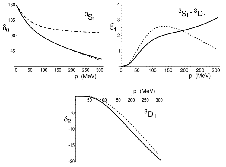
FIG. 8.: The phase shifts $\delta_{0}$, $\delta_{2}$ and mixing parameter $\varepsilon_{1}$ for the ${}^{3}\kern-1.4ptS_{1}-{}^{3}\kern-1.4ptD_{1}$ channel. The solid line denotes the results of the Nijmegen partial wave analysis. The dot-dashed curve is the fit at $O(Q^{-1})$ for $\delta_{0}$, while $\delta_{2}=\varepsilon_{1}=0$ at this order. The dashed curves are the results of the $O(Q^{0})$ fit of $\delta_{0}$ to the partial wave analysis over the momentum range $p\leq 200\ {\rm\ MeV}$, as given in eq. (97).

D Higher partial waves

The analysis of the previous section demonstrates how the power counting impacts the ${}^{3}\kern-1.4ptD_{1}$ channel and this discussion generalizes to other partial waves. A local operator that connects an angular momentum $L$ state with an angular momentum $L^{\prime}$ state involves at least $L+L^{\prime}$ spatial derivatives. The case of $S$-wave to $S$-wave scattering has been described in the previous sections. If either $L$ or $L^{\prime}$ but not both correspond to an $S$-wave then the operator enters at $O(Q^{L+L^{\prime}-1})$. However, if neither $L$ nor $L^{\prime}$ is equal to zero the operator contributes at $O(Q^{L+L^{\prime}})$ for $L,L^{\prime}$ odd and $O(Q^{L+L^{\prime}-1})$ for $L,L^{\prime}$ even. The contribution of pions is at $O(Q^{0})$, and is therefore the leading contribution to all non $S$-wave to $S$-wave scattering amplitudes. This contribution has been presented in the literature (e.g. [33]).

E Radiation pions and operator mixing

We have seen that graphs involving potential pion exchange occur at $O(Q^{0})$ in both the ${}^{1}\kern-1.4ptS_{0}$ and ${}^{3}\kern-1.4ptS_{1}-{}^{3}\kern-1.4ptD_{1}$ channels. Such contributions arise from kinematic regions where the intermediate nucleons are near their mass-shell, with the pion exchanged in the $t$-channel far from its pole. Contributions arising from radiation pions (the pion pole) exchanged in the $s,t$ and $u$ channels arise at $O(Q^{1})$ (for discussion of radiation exchanges in nonrelativistic gauge theories see [26, 27, 28, 29, 30, 31]). An interesting feature of virtual radiation pions in the $s$-channel is that they can cause mixing between four-nucleon operators in different spin channels. This is because the two nucleons in a virtual intermediate $NN\pi$ state can rescatter while in a different isospin and angular momentum state than the physical incoming nucleon pair.

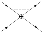
FIG. 9.: A graph involving a radiation pion that gives rise to mixing between the ${}^{1}\kern-1.4ptS_{0}-{}^{3}\kern-1.4ptS_{1}$ operators. This graph with an insertion of $(N^{\dagger}\sigma^{a}N)^{2}$ at the vertex gives the expression $\Gamma_{1}$ in eqs. (99-101).

As an example, consider the graph shown in Fig. 9 with an insertion of the operator $(N^{\dagger}\sigma^{a}N)^{2}$, denoted by $\Gamma_{1}$. Explicitly,

$$\Gamma_{1} = i{g_{A}^{2}\over 2f^{2}}N^{\dagger}\tau^{a}\sigma^{i}\sigma^{k}NN^{\dagger}\tau^{a}\sigma^{k}\sigma^{j}N$$ (99)

$$\left({\mu\over 2}\right)^{4-D}\int{d^{D}q\over(2\pi)^{D}}{q^{i}q^{j}\over\left[q^{0}+{E\over 2}-{({\bf p+q})^{2}\over(2M)}+i\epsilon\right]\left[q^{0}+{E\over 2}-{({\bf p^{\prime}+q})^{2}\over(2M)}+i\epsilon\right]\left[(q^{0})^{2}-{\bf q}^{2}-m_{\pi}^{2}+i\epsilon\right]}\ .$$

The $q^{0}$ integral is performed by forming a contour enclosing the one pole in the upper half of the complex plane provided by the pion propagator. Using the equations of motion $E={\bf p}^{2}/M+O({\bf p}^{4}/M^{3})$ and neglecting the $O({\bf p}^{4}/M^{3})$ relativistic correction we realize that the weight of the integral in the low energy theory will be for momentum near the pion mass and perform an expansion in $1/M$, giving

$$\Gamma_{1} = {g_{A}^{2}\over 4f^{2}}N^{\dagger}\tau^{a}\sigma^{i}\sigma^{k}NN^{\dagger}\tau^{a}\sigma^{k}\sigma^{j}N\left({\mu\over 2}\right)^{4-D}\int{d^{D-1}q\over(2\pi)^{D-1}}{q^{i}q^{j}\over\left[{\bf q}^{2}+m_{\pi}^{2}\right]^{3\over 2}}\ +\ O(1/M)\ .$$ (100)

Evaluating the integral yields

$$\Gamma_{1} = {3g_{A}^{2}m_{\pi}^{2}\over 32\pi^{2}f^{2}}\left[{1\over\epsilon}-\log\left({m_{\pi}^{2}\over\mu^{2}}\right)+{\rm constant}\right]\left[\left(N^{\dagger}\sigma^{a}N\right)^{2}\ +\ \left(N^{\dagger}N\right)^{2}\right]\ +\ O(1/M)\ .$$ (101)

Including all the irreducible graphs and wavefunction renormalization it is straightforward to find the leading radiation pion contribution to the $\beta$ functions for $D_{2}^{({}^{1}\kern-0.98ptS_{0})}$ and $D_{2}^{({}^{3}\kern-0.98ptS_{1})}$ are

$$\beta_{D_{2}^{({}^{1}\kern-0.7ptS_{0})}}^{(rad)} = +\ {3g_{A}^{2}\over 4\pi^{2}f^{2}}\left(C_{0}^{({}^{3}\kern-0.98ptS_{1})}-C_{0}^{({}^{1}\kern-0.98ptS_{0})}\right)\ \ \ ,$$ (102)

$$\beta_{D_{2}^{({}^{3}\kern-0.7ptS_{1})}}^{(rad)} = -\ {3g_{A}^{2}\over 4\pi^{2}f^{2}}\left(C_{0}^{({}^{3}\kern-0.98ptS_{1})}-C_{0}^{({}^{1}\kern-0.98ptS_{0})}\right)\ .$$ (103)

These contributions give rise to mixing between the $S$-wave spin-singlet and spin-triplet operators.

F Relativistic effects

A further contribution starting at $O(Q^{1})$ arises from relativistic corrections to the energy-momentum relation. A detailed discussion of such effects in dimensionally regulated non-relativistic gauge theories can be found in [29] and the situation is similar for nucleon interactions. Neglecting pion fields, the lagrange density in the single nucleon sector is

$${\cal L} = N^{\dagger}\left(i\partial_{0}+{\nabla^{2}\over 2M}\right)N\ +\ {1\over 8M^{3}}N^{\dagger}\nabla^{4}N\ +\ ...\ ,$$ (104)

where the spatial gradient operator brings down factors of ${\bf p}$. It is understood that the $N^{\dagger}\nabla^{4}N$ operator is inserted perturbatively into graphs, e.g. Fig. 10, and that the lowest order equations of motion are modified to $E/2={\bf p}^{2}/2M+{\bf p}^{4}/8M^{3}+\ldots$. A single insertion of $N^{\dagger}\nabla^{4}N$ gives rise to a $O(Q^{1})$ contribution; however, it is suppressed by factors of the nucleon mass and not $\Lambda_{NN}$. Consequently, its effect is expected to be small compared to other corrections at this order.

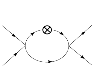
FIG. 10.: Higher dimension operators arising from relativistic corrections to the energy-momentum relation, denoted by the crossed-circle, are inserted perturbatively.

IV Overview

In a previous letter [2] we presented a new power counting scheme to describe NN scattering processes that does not suffer from the inconsistencies of Weinberg’s scheme [3]. In order to achieve consistent power counting a new subtraction scheme is used for dimensionally regulated integrals, designed to keep track of power law divergences in theories in which there are delicate cancellations at short distance; for $NN$ scattering, these cancellations manifest themselves as a large scattering length. The renormalization group provides a powerful tool in the analysis of such theories and allows one to identify the order at which a given operator will contribute.

In the present paper we have elaborated on our expansion, with particular emphasis on the utility of the renormalization group. We have also presented detailed analytic computations for $NN$ scattering in the ${}^{1}\kern-1.4ptS_{0}$ and ${}^{3}\kern-1.4ptS_{1}-{}^{3}\kern-1.4ptD_{1}$ channels, complete to the subleading $O(Q^{0})$ order, and have shown that the agreement with experiment at low energy is quite good. A particular success was the calculation of the ${}^{3}\kern-1.4ptS_{1}-{}^{3}\kern-1.4ptD_{1}$ mixing parameter $\varepsilon_{1}$ shown in Fig. 8, with no free parameters. We then discussed the power counting for higher partial waves, and showed that they are dominated by pion exchange in the Born approximation. Finally, we showed how to deal with relativistic effects and virtual radiative pions, which are features that arise at order $O(Q^{1})$.

The techniques presented here should be applicable to a number of low energy processes, such as radiative capture, and electromagnetic moments of the deuteron. Theoretical challenges include extending the validity of the expansion above the scale $\Lambda_{NN}$, and applying the technique to systems with three or more nucleons.

We would like to thank G. Bertsch for useful discussions. This work is supported in part by the U.S. Dept. of Energy under Grants No. DOE-ER-40561, DE-FG03-97ER4014, and DE-FG03-92-ER40701.

REFERENCES

• [1] A.V. Manohar, Lectures given at 35th Internationale Universitatswochen fuer Kern- und Teilchenphysik, Perturbative and Nonperturbative Aspects of Quantum Field Theory, Schladming, Austria, 2-9 Mar 1996. hep-ph/9606222 .
• [2] D.B. Kaplan, M.J. Savage and M.B. Wise, nucl-th/9801034, to appear in Phys. Lett. B.
• [3] S. Weinberg, Phys. Lett. B251 (1990) 288; Nucl. Phys. B363 (1991) 3; Phys. Lett. B295 (1992) 114.
• [4] C. Ordonez and U. van Kolck, Phys. Lett. B291 (1992) 459; C. Ordonez, L. Ray and U. van Kolck, Phys. Rev. Lett. 72 (1994) 1982; Phys. Rev. C53 (1996) 2086.; U. van Kolck, Phys. Rev. C49 (1994) 2932.
• [5] T.S. Park, D.P. Min and M. Rho, Phys. Rev. Lett. 74 (1995) 4153; Nucl. Phys. A596 (1996) 515.
• [6] D.B. Kaplan, M.J. Savage and M.B. Wise, Nucl. Phys. B478 (1996) 629, nucl-th/9605002.
• [7] T. Cohen, J.L. Friar, G.A. Miller and U. van Kolck, Phys. Rev. C53 (1996), 2661.
• [8] D. B. Kaplan, Nucl. Phys. B 494 (1997) 471.
• [9] T.D. Cohen, Phys. Rev. C55 (1997) 67. D.R. Phillips and T.D. Cohen, Phys. Lett. B390 (1997) 7. K.A. Scaldeferri, D.R. Phillips, C.W. Kao and T.D. Cohen, Phys. Rev. C56 (1997) 679. S.R. Beane, T.D. Cohen and D.R. Phillips, nucl-th/9709062.
• [10] J.L. Friar, Few Body Syst. 99 (1996) 1, nucl-th/9607020.
• [11] M.J. Savage, Phys. Rev. C55 (1997) 2185, nucl-th/9611022.
• [12] M. Luke and A.V. Manohar, Phys. Rev. D55 (1997) 4129, hep-ph/9610534 .
• [13] G.P. Lepage, nucl-th/9706029, Lectures given at 9th Jorge Andre Swieca Summer School: Particles and Fields, Sao Paulo, Brazil, 16-28 Feb 1997.
• [14] S.K. Adhikari and A. Ghosh, J. Phys. A30 (1997) 6553.
• [15] K.G. Richardson, M.C. Birse and J.A. McGovern, hep-ph/9708435.
• [16] P.F. Bedaque and U. van Kolck, nucl-th/9710073; P.F. Bedaque, H.-W. Hammer and U. van Kolck, nucl-th/9802057.
• [17] T.S. Park, K. Kubodera, D.P. Min and M. Rho, hep-ph/9711463.
• [18] M. J. Savage and M. B. Wise, Phys. Rev. D53 (1996), hep-ph/9507288.
• [19] D.B. Kaplan and A.E. Nelson, Phys. Lett. B175 ( 1986) 57; A. E. Nelson and D. B. Kaplan, Phys. Lett. 192B (1987) 193.
• [20] H.D. Politzer and M.B. Wise, Phys. Lett. B257 (1991) 399; G.E. Brown, C.-H. Lee, M. Rho, V. Thorsson, Nucl. Phys. A567 (1994) 937; C.M. Ko, V. Koch and G. Li, nucl-th/9702016; G.Q. Li, C.H. Lee and G.E. Brown, Nucl. Phys. A625 (1997) 372, nucl-th/9706057.
• [21] J. Gegelia, nucl-th/9802038.
• [22] S. Weinberg, Phys. Rev. Lett. 17 (1966) 616; Phys. Rev. 166 (1968) 1568.
• [23] A. Manohar and H. Georgi, Nucl. Phys. B234 (1984) 189.
• [24] J. Gasser and H. Leutwyler, Annals Phys. 158 (1984) 142; Nucl. Phys. B250 (1985) 465.
• [25] A. G. Cohen, D.B. Kaplan and A.E. Nelson, Phys. Lett. B412 301, hep-ph/9706275
• [26] M. Luke and A.V. Manohar, Phys. Lett. B286 (1992) 348, hep-ph/9205228
• [27] P. Labelle, hep-ph/9608491
• [28] B. Grinstein and I.Z. Rothstein, Phys. Rev. D57 (1998) 78. hep-ph/9703298
• [29] M. Luke and M.J. Savage, Phys. Rev. D57 (1998) 413. hep-ph/9707313.
• [30] M. Beneke and V.A. Smirnov, hep-ph/9711391
• [31] H.W. Griesshammer, hep-ph/9712467.
• [32] V.G.J. Stoks, R.A.M. Klomp, C.P.F. Terheggen and J.J. de Swart, Phys. Rev. C49 (1994) 2950, nucl-th/9406039.
• [33] Pions and Nuclei by T. Ericson and W. Weise, Oxford Science Publications (1988); ISBN 0-19-852008-5.