Analysis of Eta Production using a Generalized Lee Model

Abstract

We have investigated the processes N($\pi$, $\pi$)N and N($\pi$, $\eta$)N close to eta threshold using a simple, nonrelativistic Lee model which has the advantage of being analytically solvable. It is then possible to study the Riemann sheets of the S-matrix and the behavior of its resonance poles especially close to threshold. A theoretical simulation of the experimental cusp effect at eta threshold leads to a characteristic distribution of poles on the Riemann sheets. We find a pole located in the $4^{th}$ Riemann sheet that up to now has not been discussed. It belongs to the cusp peak at eta threshold. In addition we obtain the surprising result using the Lee model that the resonance $S_{11}(1535)$ does not play a large role. The main features of the experimental data can be reproduced without explicitly introducing this resonance. Furthermore, we have also studied the reactions N($\gamma$, $\pi$)N and N($\gamma$, $\eta$)N and find reasonable agreement between the data and both models with and without the $S_{11}(1535)$ resonance.

PACS numbers: 13.60.Le, 14.20.Gk, 13.75.Gx

Keywords: Lee model, $S_{11}(1535)$, eta production

I Introduction

The advent of new electron accelerators and intense photon sources substantially improved the data basis of electron and photoproduction of eta mesons. High quality data for angular distributions and total cross sections for photon energies between threshold and 790 MeV may be considered a qualitative breakthrough in the experimental field. The progress in experimental proficiency demands a better theoretical understanding of these processes.

The eta meson is believed to be mainly produced by the resonance $S_{11}(1535)$ which is located close to eta threshold (1486 MeV). Considerable work has been done in the case of eta photoproduction [1], [2], [3] with the $S_{11}(1535)$ resonance as the main production channel.

The eta threshold also influences scattering cross sections other than eta production. This is especially true in elastic pion scattering where a strong cusp effect is observed due to unitarity. The presence of this cusp makes it difficult to get information on the resonance $S_{11}(1535)$, because the cusp and the resonance have similar signatures when analyzing experimental data. Even the existence of the resonance $S_{11}(1535)$ seems to be questionable [4], [5]. In a recent coupled channel calculation for eta and kaon photoproduction, Kaiser et al. [6] have shown that the $S_{11}(1535)$ can as well be explained as a quasi-bound state of kaon/$\Sigma$-hyperon.

It is generally accepted that the $S_{11}(1535)$ couples strongly to the eta while the neighboring resonance $S_{11}(1650)$ for all practical purposes does not decay into eta mesons. It is not clear why these two neighboring resonances, having the same quantum numbers, behave so differently.

We investigated theoretically the combination of a resonance and the threshold effect using a Lee model because of its simplicity and clearness. It is fully analytically solvable, unitary and can in principle be extended to an arbitrary number of different mesons and resonances. The absence of antiparticles makes the model nonrelativistic. However, a covariant formalism of resonance excitation also leads to problems, e.g. anti-resonances ($\bar{q}\bar{q}\bar{q}$) that are very unlikely in terms of quark models. Analyticity is mainly due to an inherent Tamm-Dancoff approximation in the model which limits the number of mesons present at any instant.

Our model describes the interaction of the nucleon, the two resonances $S_{11}(1535)$ and $S_{11}(1650)$, the pion and the eta meson. Making use of perturbation theory we also included photoproduction of pions and eta mesons. From our calculation we find that two-pion production can not entirely be neglected. It was accounted for in a simple manner as discussed in the sect. III. Coupling constants used in our model were determined by fitting to experimental data from pion scattering experiments and eta (pion) photoproduction.

It is especially interesting to study the scattering matrix S. It is defined on several Riemann sheets of the complex energy plane. One finds that poles of S are distributed in a characteristic way on these sheets and can be identified with objects like resonances or the cusp.

The Lee model was introduced in 1954 by T.D. Lee to study questions concerning renormalization of field theories [7]. Pauli, Glaser and Källén [8], [9] used this model in order to investigate the appearance of “ghost states”, states of negative probability density. Ghost states appear when coupling constants are chosen to be large. This lead to the discussion of the meaning of an indefinite metric in a Hilbert space. Höhler [10] used the Lee model for a quantum mechanical examination of the exponential decay law of unstable particles. The Lee model has not been extensively utilized for decades. A good introduction can be found in [11] and [12]. Using the Lee model our main goal was not the perfect description of experimental data but to investigate the interplay and meaning of both cusp effect and resonance $S_{11}(1535)$ at threshold.

We find that in order to properly treat the threshold effect, rescattering and calculation to all orders of perturbation theory is essential. A simple Born approximation at eta threshold is insufficient. We show which Riemann sheets should be considered when looking for resonance poles on the complex energy plane. The sheet structure plays an important role at threshold.

From the fact that the experimental data can be roughly described without explicitly using the resonance $S_{11}(1535)$, we think that the importance of this resonance is commonly overestimated and threshold effects must be taken into account.

In the following we give an introduction to the generalized Lee model. We then discuss the fit results together with the experimental data. First we consider the production of eta mesons when pions are scattered by a nucleon. Finally we treat eta and pion photoproduction.

II A Generalized Lee Model

According to the quantum numbers of the $S_{11}(1535)$ resonance, eta production happens mainly in a s-wave channel. Since angular momentum and isospin are conserved quantities in strong interaction, we can also restrict our calculation to the Hilbert subspace where L = 0 and I = 1/2. Furthermore, we work in the center of momentum system. These choices considerably simplify our calculations.

The particles that appear in our model are the nucleon N, the two resonances $R_{1}$ and $R_{2}$ (namely $S_{11}(1535)$ and $S_{11}(1650)$) and the two mesons $M_{1}$ and $M_{2}$ (pion and eta). Taking the quantum numbers in isospin space to be $I=1/2$ and $I_{z}=1/2$, the nucleon pion state is actually a superposition of the physical pion states:

$$\mid N,\pi,I=1/2,I_{z}=1/2\rangle={1\over\sqrt{3}}\left(\sqrt{2}\mid n\rangle\mid\pi^{+}\rangle-\mid p\rangle\mid\pi^{o}\rangle\right).$$ (1)

We adopt the following notation, so that the isospin does not appear explicitly:

$$\mid N,\pi\rangle=\mid N,\pi,I=1/2,I_{z}=1/2\rangle\,.$$ (2)

Because we want to make full use of the isospin formalism we have the difficulty of attributing masses to the pion and the nucleon since the physical particles ($\pi^{o}$, $\pi^{+}$) and ($n$, $p$) all have different masses. We chose average masses $m_{\pi}=137$ MeV and $m_{N}=939$ MeV.

The mesons and the nucleon are treated as stable particles. However, the resonances $S_{11}(1535)$ and $S_{11}(1650)$ are not stable, because of the decay into nucleon and mesons. This leads to a “dressing” of resonances, e.g. the physical resonances are surrounded by a cloud of virtual mesons. In our calculation we use the bare resonance states - not the physical ones. Therefore the masses of the resonances, $m_{Rj}$, that appear in the model are bare masses and are used as fit parameters in the model.

The following self adjoint Hamiltonian describes the five particles and their interactions. It consists of two parts, the free Hamiltonian and the interaction term:

$$H=H_{o}+H_{int}\,,$$ (3)

so that

$$H_{o}\mid R_{j}\rangle = m_{Rj}\mid R_{j}\rangle\,,$$ (4)

$$H_{o}\mid N(-\vec{k}),M_{l}(\vec{k})\rangle = W_{l}\mid N(-\vec{k}),M_{l}(\vec{k})\rangle\,,$$ (5)

where $W_{l}$ is the total energy in the center of momentum (c.m.) system,

$$W_{l}=\sqrt{m_{l}^{2}+\vec{k}^{2}}+\sqrt{m_{N}^{2}+\vec{k}^{2}}.$$ (6)

$\vec{k}$ is the momentum of particles in the c.m. system. We distinguish two sorts of interaction among the particles: “resonance interaction” and “contact interaction” (see Fig. 1). In the resonance interaction a meson and a nucleon combine to form a resonance, or a resonance disintegrates into a meson and a nucleon

$$R_{j}\quad\Longleftrightarrow\quad N,M_{l}\,,$$

$$\langle R_{j}\mid H_{int}\mid N(-\vec{k}),M_{l}(\vec{k})\rangle = g^{R}_{j,l}~{}F_{l}(W_{l})\,.$$ (7)

The index $l$ is used for mesons, index $j$ refers to resonances and $g^{R}_{j,l}$ is the respective coupling constant. $F_{l}(W_{l})$ is a real cut-off form factor which is introduced to assure convergence of expressions that will appear later in the calculations for the cross sections. It determines how the interaction between the particles weakens as the kinetic energy rises.

The contact interaction on the other hand corresponds to a nonresonant interaction, ingoing mesons are scattered into outgoing mesons,

$$N,M_{l}\quad\Longleftrightarrow\quad N,M_{l^{\prime}}\,,$$

$$\langle N,M_{l}(\vec{k})\mid H_{int}\mid N,M_{l^{\prime}}(\vec{k}^{\prime})\rangle={g_{l^{\prime},l}\over m_{\pi}}~{}F_{l^{\prime}}(W^{\prime}_{l^{\prime}})~{}F_{l}(W_{l})\,.$$ (8)

The coupling constants $g_{l,l^{\prime}}$ for the contact interaction term are symmetric, e.g. $g_{l,l^{\prime}}=g_{l^{\prime},l}$.

Fig. 1 shows the vertices for these interactions. The cut-off function $F_{l}(W_{l})$ is taken to be the same for the resonance and contact interaction terms. This is arbitrary, but it simplifies the calculations. In our computer simulations (see sect. II B) we chose $F_{l}(W_{l})$ to be a simple analytical function in order to keep computation time short. In principal, $F_{l}$ can also be deduced from more advanced models by evaluating the matrix elements in Eqs. 7 and 8.

To determine the energy eigenstates of the total Hamiltonian $H$, we write

$$H~{}\mid N,M_{i}(\vec{k})\rangle_{+}=W~{}\mid N,M_{i}(\vec{k})\rangle_{+}\,,$$ (9)

where $\mid N,M_{i}(\vec{k})\rangle_{+}$ is a scattering state which satisfies the Lippmann-Schwinger equation for ingoing boundary conditions,

$$\mid N,M_{i}(\vec{k})\rangle_{+}=\mid N,M_{i}(\vec{k})\rangle-\frac{1}{H_{o}-W-i\epsilon}H_{int}\mid N,M_{i}(\vec{k})\rangle_{+}~{}.$$ (10)

$M_{i}$ stands for the incident meson ($i=$incident) that at time $t=-\infty$ comes in as a plane wave. The Lippmann-Schwinger equation can be solved using the following ansatz,

$$\mid N,M_{i}(\vec{k})\rangle_{+}=\sum_{j}\beta^{i}_{j}\mid R_{j}\rangle+\sum_{l}\int d^{3}k^{\prime}~{}\alpha^{i}_{l}(\vec{k}^{\prime})\mid N,M_{l}(\vec{k}^{\prime})\rangle\,.$$ (11)

The coefficients $\alpha$ and $\beta$ in Eq. (11) can be obtained by multiplying from the left with $\langle R_{j}\mid,~{}\langle N,M_{l}\mid$ and using the orthonormality of the basis. If we define

$$t^{i}_{l} = \int d^{3}k~{}F_{l}(W_{l})\alpha^{i}_{l}(\vec{k})\,,$$ (12)

we get

$$\beta^{i}_{j}=-\frac{1}{m_{Rj}-W}\cdot\sum_{l}g^{R}_{j,l}~{}t^{i}_{l}\,,$$ (13)

$$\alpha^{i}_{l}(\vec{k}) = \delta(\vec{k}-\vec{k}_{i})\delta_{l,i}+\frac{F_{l}(W_{l})}{W-W_{l}+i\epsilon}\cdot\sum_{l^{\prime}}t^{i}_{l^{\prime}}G_{l^{\prime}l}\,,$$ (14)

where

$$G_{l^{\prime}l} = \sum_{j}\frac{g^{R}_{j,l^{\prime}}\,g^{R}_{j,l}}{m_{Rj}-W}-{g_{l^{\prime},l}\over m_{\pi}}\,,$$ (15)

$G_{l^{\prime}l}$ can be considered as an effective coupling constant. It is energy dependent and symmetric, $G_{l^{\prime}l}=G_{l^{\prime}l}(W)=G_{ll^{\prime}}$.

After inserting (14) into (12) one obtains:

$$\sum_{l^{\prime}}h_{ll^{\prime}}t^{i}_{l^{\prime}}=\delta_{i,l}F_{i}(W)$$ (16)

with

$$h_{ll^{\prime}}=\delta_{l,l^{\prime}}-H_{l}G_{ll^{\prime}}$$ (17)

and

$$H_{l}=H_{l}(W)=\int d^{3}k~{}\frac{F_{l}^{2}(W_{l})}{W_{l}-W-i\epsilon}\,.$$ (18)

Eq. (16) is a system of linear equations for $t^{i}_{l}$ which can be solved by standard mathematical methods. We note that in the derivation of Eq. (16) the number of different resonances and mesons in the model is arbitrary. If for example n different mesons are involved in the scattering process, a $n\times n$ matrix needs to be inverted. When solving for $t^{i}_{l}$ one encounters an important function which we call $h_{det}$. It is the determinant of $h_{ll^{\prime}}$ in Eq. (16) and contains most of the information of the scattering process. It is a function of $G_{ll^{\prime}}$ and $H_{l}$. As will be shown $h_{det}$ as well as $H_{l}$ are meromorphic functions of $W$. They are defined on several Riemann sheets.

Once the $t_{l}^{i}$ are determined the scattering amplitude $T_{fi}$ can be calculated,

$$T_{fi}=~{}\langle N,M_{f}(k_{f})\mid H_{int}\mid N,M_{i}(k_{i})\rangle_{+}=-F_{f}(W)\sum_{l^{\prime}}G_{fl^{\prime}}~{}t^{i}_{l^{\prime}}\,,$$ (19)

where $f$ and $i$ stand for outgoing and incoming mesons respectively.

A An example

In order to familiarize the reader with the Lee model, we present here a simple and instructive example that shows the principal features of the general Lee model. We will calculate scattering amplitudes, cross sections and the scattering matrix, which will all appear in their familiar textbook forms.

We consider the case where the two mesons, $\pi$ and $\eta$, couple only to one resonance $R_{1}$ (resonance interaction) without contact interactions. The coefficients $\alpha$ and $\beta$ of the scattering state are then found to be

$$\alpha^{i}_{l}(k) = \delta(\vec{k}-\vec{k}_{i})~{}\delta_{l,i}-\beta^{i}~{}g^{R}_{1,l}~{}F_{l}(W_{l})~{}\frac{1}{W_{l}-W-i\epsilon},$$ (20)

$$\beta^{i} = -g^{R}_{1,i}F_{i}(W)~{}\frac{1}{h_{det}}\,,$$ (21)

where $h_{det}$ is the determinant mentioned before:

$$h_{det}=h_{det}(W) = m_{R}-W-\sum_{l}(g^{R}_{1,l})^{2}H_{l}\,.$$ (22)

We immediately obtain expressions for the scattering amplitude $T_{fi}$ and the scattering cross section

$$T_{fi} = ~{}\langle N,M_{f}(k_{f})\mid H_{int}\mid N,M_{i}(k_{i})\rangle_{+}$$ (23)

$$= \displaystyle-g^{R}_{1,i}~{}g^{R}_{1,f}~{}{F_{f}(W)F_{i}(W)\over h_{det}}\,.$$ (24)

Using Fermi’s rule we obtain the cross section

$$\frac{d\sigma}{d\Omega} = \frac{2\pi}{\hbar}\frac{1}{\mid\vec{j}_{in}\mid}\mid T_{fi}\mid^{2}\varrho(W)\,,$$ (25)

where $\vec{j}_{in}$ is the incoming flux and $\varrho(W)$ is the phase space density of the outgoing state.

After taking a closer look at the $H_{l}$ we can write the scattering cross section in a very convenient form. We take $H_{l}$ as in Eq. (18) and make use of the identity

$$\frac{1}{W_{l}-W\mp i\epsilon}=P\frac{1}{W_{l}-W}\pm i\pi~{}\delta(W_{l}-W)\,,$$ (26)

where P stands for the principal value. Let us write

$$(g^{R}_{1,l})^{2}~{}H_{l} = \Delta_{l}+i~{}\Gamma_{l}/2\,,$$ (27)

where we set

$${\Gamma_{l}\over 2} = 4\pi^{2}~{}(g^{R}_{1,l})^{2}~{}F_{l}^{2}(W)~{}k_{l}\frac{\omega_{l}~{}E_{N}}{W}~{}\Theta(W-m_{l}-m_{N})\,,$$ (28)

$$\Delta_{l} = 4\pi~{}(g^{R}_{1,l})^{2}~{}P\int_{m_{l}+m_{N}}^{\infty}dW_{l}{F^{2}_{l}(W_{l})\over W_{l}-W}k_{l}\frac{\omega_{l}~{}E_{N}}{W_{l}}\,,$$ (29)

and $\omega_{l}=\sqrt{m_{l}^{2}+\vec{k}^{2}_{l}}$ and $E_{N}=\sqrt{m_{N}^{2}+\vec{k}^{2}_{l}}$. $\Gamma_{l}$ turns out to be the partial width of the resonance for the decay channel into meson $l$ and the nucleon. The step function $\Theta$ in the expression for $\Gamma_{l}$ leads to a zero partial width below threshold of meson $l$, and $\Delta_{l}$ can be interpreted as the mass shift of the resonance due to its interaction with the mesons.

This can be clearly seen when we look at the expression for the scattering cross section that we finally obtain:

$$\frac{d\sigma}{d\Omega} = \displaystyle{1\over k_{i}^{2}}\left|\displaystyle{\displaystyle\sqrt{\Gamma_{i}\Gamma_{f}/4}\over h_{det}}\right|^{2}$$ (30)

$$= {1\over k_{i}^{2}}\displaystyle{\displaystyle\Gamma_{i}\Gamma_{f}/4\over(m_{R}-\Delta_{\pi}-\Delta_{\eta}-W)^{2}+(\Gamma_{\pi}/2+\Gamma_{\eta}/2)^{2}}\,.$$ (31)

The cross section has the well known Breit-Wigner form of a resonance. We note, that the total Breit-Wigner width of the resonance, $\Gamma_{tot}$, is the sum of the partial widths, $\Gamma_{\pi}+\Gamma_{\eta}$. The physical mass of the resonance, $m_{R}-\Delta_{\pi}-\Delta_{\eta}$, is composed of the bare mass of the resonance $m_{R}$ and the “mass shifts” $\Delta_{\pi}$ and $\Delta_{\eta}$. The physical mass of the resonance is lowered by the coupling to the mesons. The partial “mass shifts” of the resonance, $\Delta_{l}$, add up to give a total mass shift. It is interesting to note that the same function $F_{l}$ that cuts off the interaction between the particles also is the cut-off for the width $\Gamma_{l}$. $F_{l}$ is supposed to be a smooth function that gradually falls off as $W$ increases. We then reckon that the widths $\Gamma_{l}$ grow proportionally to $k_{l}(W)$ at their respective $l$-meson threshold when $W$ is increased. This is in agreement with general scattering theory that predicts the same behavior for s-wave resonances.

The S-matrix is a $2\times 2$ matrix which corresponds to the two reaction channels. One finds

$${\bf S_{o}}=\left(\begin{array}[]{cc}\displaystyle 1+\frac{i\Gamma_{\pi}}{h_{det}}&\displaystyle\frac{i\sqrt{\Gamma_{\pi}\Gamma_{\eta}}}{h_{det}}\cr\displaystyle\frac{i\sqrt{\Gamma_{\pi}\Gamma_{\eta}}}{h_{det}}&\displaystyle 1+\frac{i\Gamma_{\eta}}{h_{det}}\cr\end{array}\right).$$

$S_{o}$ is unitary and the off-diagonal elements are equal which corresponds to time inversion symmetry. From $S_{o}$ one can easily determine the scattering phases by comparing it to the textbook form of a two channel S-matrix:

$${\bf S_{o}}=\left(\begin{array}[]{cc}\displaystyle\xi~{}e^{2i\delta_{1}}&\displaystyle i\sqrt{1-\xi^{2}}~{}e^{i(\delta_{1}+\delta_{2})}\cr\displaystyle i\sqrt{1-\xi^{2}}~{}e^{i(\delta_{1}+\delta_{2})}&\displaystyle\xi~{}e^{2i\delta_{2}}\cr\end{array}\right),$$

where $\xi$ is the inelasticity and $\delta_{1/2}$ are the elastic scattering phases.

B The Form Factor $F_{l}$

The cut-off functions $F_{l}$ are constructed so that at low energies their values are constant. With increasing energy the interaction between the particles gradually decreases. It seems reasonable that at the c.m. energy of about two nucleon masses the interaction should be strongly suppressed.

Although there are many different cut-off functions which fulfill these features it turns out that in general they produce similar results. We selected a cut-off function simple enough so that the integrals $H_{l}$ could be calculated analytically. Explicitly we fixed the cut-off function such that

$$H_{l}(W) = \int d^{3}k\frac{F_{l}^{2}(W_{l})}{W_{l}-W}$$ (32)

$$= \sqrt{2m_{l}}\int_{m_{l}+m_{N}}^{C}dW_{l}{\sqrt{W_{l}-m_{l}-m_{N}}\over W_{l}-W}\,,$$ (33)

where $C$ is a cut-off parameter. $C$ was chosen to be 2000 MeV, so the interaction of the meson with the nucleon stops abruptly for $W_{l}>C$. We now show that $H_{l}$ (as a complex function) is defined on two Riemann sheets.

Let us consider $W$ in Eq. (33) as a complex variable. $H_{l}$ is then two sheeted and has a cut from $m_{l}+m_{N}$ to $C$. The easiest way to see this is by approaching the real axis from above and below and making use of the identity (26). The continuation of $H_{l}$ into its second sheet can be done by contour deformation of the integral and applying Cauchy’s residue theorem. Explicitly we find:

$$H_{l}(W)\mid_{1.sheet} = 2\sqrt{2m_{l}}\sqrt{C-m_{l}-m_{N}}$$ (34)

$$- 2\sqrt{2m_{l}}\sqrt{m_{l}+m_{N}-W}~{}\arctan({\sqrt{C-m_{l}-m_{N}}\over\sqrt{m_{l}+m_{N}-W}})\,,$$ (35)

$$H_{l}(W)\mid_{2^{nd}sheet} = H_{l}(W)\mid_{1^{st}sheet}+~{}2\pi\sqrt{2m_{l}}\sqrt{m_{l}+m_{N}-W}\,.$$ (36)

$H_{l}$ diverges at $W=C$ because of the step of the cut-off at $C$. In our simulations we always stayed well below $C$.

Under the condition $C-m_{l}-m_{N}>>\mid m_{l}+m_{N}-W\mid$, we can approximate

$$H_{l}(W)\mid_{2^{nd}sheet} \approx 2\sqrt{2m_{l}}\sqrt{C-m_{l}-m_{N}}+\pi\sqrt{2m_{l}}\sqrt{m_{l}+m_{N}-W}\,.$$ (37)

The expression $\sqrt{m_{l}+m_{N}-W}$ is directly related to the partial width of the resonance $\Gamma_{l}$ as defined in sect. II A. At threshold, e.g. $m_{l}+m_{N}=W$, $\sqrt{m_{l}+m_{N}-W}$ becomes imaginary and grows like the meson momentum $k_{l}$ with increasing energy $W$.

C The S-matrix

We can get a better understanding of the physics underlying the scattering and production processes by studying the S-matrix $S_{o}$. We will show in the following how poles of the scattering matrix can be identified with resonance peaks or cusp peaks in physical cross sections. It will become clear that the distribution of poles and their location on different Riemann sheets gives valuable information on the physics involved. We can take full advantage of the fact that the Lee model is analytically solvable. Important features of the S-matrix are determined by general physical laws like unitarity, causality, time reversal invariance and symmetries of the interactions. A very good introduction to the subject can be found in the books by Nussenzveig and Bohm [13], [14]. In the following we consider the S-matrix as a complex function of the energy $W$. S is then found to be meromorphic and is defined on several Riemann sheets. It is mainly determined by the determinant $h_{det}$, which is the same for all channels, e.g. in our case $N(\pi,\pi)N$, $N(\pi,\eta)N$, $N(\eta,\eta)N$ and $N(\eta,\pi)N$. For our example in sect. II A, we have

$$h_{det}=m_{R}-g^{R}_{1,\pi}H_{\pi}-g^{R}_{1,\eta}H_{\eta}-W\,,$$ (38)

i.e. $h_{det}$ is a four sheeted function, because each $H_{l}$ is defined on two sheets. There are two cuts located on the real energy axis corresponding to the two meson thresholds. They start at the respective meson production thresholds which are also the branch points for the Riemann sheets. Fig. 2 shows those four Riemann sheets of $h_{det}$, the branch points, and the cuts along the real axis. Whenever a cut is crossed one enters another Riemann sheet. Starting from the first sheet one moves into the second or third sheet depending on whether the cut was passed below or above eta threshold. Passing a sheet twice, brings you back to the original sheet. The fourth sheet can be reached from the first sheet by passing the cut twice, once below and once above eta threshold. We find poles in the complex plane that belong to the resonance, $R_{1}$, called resonance poles. The coordinates of the S-matrix poles are functions of the coupling constants. In a typical case when the coupling constants are small, the resonance poles are found in the second and the third sheet close to the bare mass $m_{R}$. Following the discussion in sect. II A, the pole coordinates will then be practically determined by the partial widths $\Gamma_{l}$ and the mass shifts $\Delta_{l}$. If the resonance peak of the scattering cross section is located above (below) eta threshold, its shape is determined by the pole in the third (second) sheet. As the coupling constants are increased the ‘virtual’ meson cloud is bound more and more tightly to the physical resonance. This lowers the physical mass of the resonance (the resonance peak moves towards the pion threshold) and increases its decay width. As a consequence the resonance pole moves away from the physical axis and towards the pion threshold (see Fig. 3). In general this behavior is the same for poles in the second or third sheet. However, if the coupling constant $g^{R}_{1,\pi}$ is held small and constant, and only the coupling of the eta meson $g^{R}_{1,\eta}$ is increased, the pole in the second sheet moves into the fourth sheet as drawn in Fig. 3. It is this pole in the fourth sheet that gives rise to the cusp peak at eta threshold. This will be of importance in the following section.

We briefly remark that if the coupling of the mesons to the resonance becomes strong enough the physical resonance finally becomes a bound state. This bound state is then represented by a pole in the first sheet on the real axis below pion threshold. Indeed, with increasing coupling constants the pole of the second sheet moves towards (and finally onto) the pion threshold where it can pass across the branch point to the first sheet. This behavior of the pole was first seen by Höhler [10] (see also in detail [15] and [16]).

III Scattering phase analysis of pion nucleon scattering

Because we work in the Hilbert subspace corresponding to quantum numbers $I=1/2$, $J=1/2$ and $L=0$, it is convenient to use a partial wave phase analysis of the experimental data to determine the parameters of our model. There is a variety of scattering phase analysis which differ partially in their results because the evaluation methods and the underlying data are often not identical. Among the best known are those from Karlsruhe Helsinki (KH, [17], [4], [18]), Carnegie-Mellon-Berkeley (CMB, [19], [20]) and from the Virginia Polytechnic Institute (VPI, [21]). In our work we used mainly the VPI analysis by Arndt and Roper which has the convenience of being supported by the SAID interactive dial-in program.

A typical Argand diagram ($T_{0}$) of the $S_{11}$ partial wave for pion nucleon scattering is depicted in Fig. 4. The data are taken from a VPI solution (Fall 93) [21]. Useful information can be obtained by studying the Argand diagram which shows how the complex scattering amplitude $T_{0}$ for pion nucleon scattering changes as the c.m. energy is increased. At low scattering energies we get $T_{0}=0$. With increasing energy $T_{0}$ first moves counterclockwise on the ‘unitarity’ circle which implies purely elastic scattering of the pion. At about the “4 o’clock” position, $T_{0}$ bends sharply inwards. This corresponds to the threshold of eta meson production. It is also at this energy that the resonance $S_{11}(1535)$ is located. The more $T_{0}$ moves into the center of the unitary circle, the more the scattering is inelastic, in our case due to the production of eta mesons and two-pion production. After a small closed loop $T_{0}$ continues in a nearly perfect half circle. It is those circular patterns in Argand diagrams that indicate the existence of a resonance [13, 14]. In our case it corresponds to the resonance $S_{11}(1650)$. However, there is no circle that corresponds to the resonance $S_{11}(1535)$. This may imply that either there is no resonance or that its circle is heavily deformed by the opening of the eta meson channel. We address this question in the next section when we fit two models, one with and the other without resonance $S_{11}(1535)$ to the experimental values of $T_{0}$.

Fig.5 shows the calculated elastic ($\sigma_{s}$) and inelastic ($\sigma_{r}$) partial wave scattering cross sections for the partial wave $S_{11}$ which have been obtained by

$$\sigma_{s} = {4\pi\over k^{2}}\mid T_{0}\mid^{2}$$ (39)

$$\sigma_{r} = {\pi\over k^{2}}\big{(}1-\mid 1+2iT_{0}\mid^{2}\big{)}\,.$$ (40)

The elastic cross section shows two peaks at about 1500 MeV and 1700 MeV. They can be linked to the resonances $S_{11}(1535)$ and $S_{11}(1650)$ respectively. The peak at 1500 MeV is located at the eta meson production threshold. Its tip is pointed; it has a cusp. The formation of the cusp is a threshold effect and is due to unitarity [22]. We show in the next section that even the entire corresponding peak at 1500 MeV can be completely explained as a threshold effect. The peak can be reproduced in a model without the resonance $S_{11}(1535)$.

In Fig. 5 we show the elastic and inelastic cross sections together with the data of Clajus and Nefkens [23] for the total cross section of eta production. From this comparison we find that the inelasticity of the pion scattering is mainly due to the production of the eta meson. For higher energies, however, the multi-pion production is no longer negligible and consists essentially of two-pion production in the energy range below 2 GeV.

Therefore, in order to reproduce the experimental data qualitatively, the Lee model should include two-pion production. However, the inherent Tamm-Dancoff approximation only allows one meson to be present at a time. We circumvented this by introducing an additional “meson particle” in our model representing a two-pion system.

We then solve the Lee model as before, only now with three different types of mesons instead of two. The third meson type stands for the pion pair. The vertices in Fig. 6 show the coupling the two-pion pair to the nucleon and the resonances. This introduces three additional coupling constants: $g^{R}_{1,2\pi},~{}g^{R}_{2,2\pi},~{}g_{2\pi,\pi}.$ At the two-pion threshold the phase space density for the two-pion particle should not increase proportionally to the momentum $k$ like for the pion or eta meson at threshold. Instead for a two-pion system the phase space density grows approximately quadratically with energy:

$$\mbox{phase space}\propto(W_{2\pi}-2\mu_{\pi}-m_{N})^{2}\,.$$ (41)

We can take this into account by choosing $H_{2\pi}$ to be

$$H_{2\pi}=\int_{2\mu_{\pi}+m_{N}}^{C_{2\pi}}dW_{2\pi}{(W_{2\pi}-2\mu_{\pi}-m_{N})^{2}\over\mu_{\pi}~{}(W_{2\pi}-W-i\epsilon)}\,.$$ (42)

The cut-off mass, $C_{2\pi}$, was chosen to be 2000 MeV in our calculation. With our method of representing two pions by one effective particle we can not describe exclusive two-pion production, but rather use this representation to explain the total reaction cross section.

By taking into account two-pion production we also change the analytic structure of the $S$-matrix. Now there is a third threshold at $2m_{\pi}+m_{N}$ and additional Riemann sheets appear. Moreover with our choice of $H_{2\pi}$ in Eq. (42), $H_{2\pi}$ is no longer a two sheeted function of $W$, but has an infinite number of sheets. However, these sheets do not play an important role in our discussion, because we are only interested in the sheet structure in the immediate vicinity of the eta threshold. The local sheet structure at eta threshold stays unchanged. Also our discussion of the Riemann sheets and the motion of poles in sect. II C is still valid. Fig. 7 shows the new Riemann sheet structure. The sheets are numbered such that the sheet structure around the eta threshold looks the same as in Fig. 2.

IV Determination of coupling constants and poles

A glance at the partial wave cross section in Fig. 5 shows that at pion threshold (far away from the first resonance) the cross section undergoes a rapid change with increasing energy. The elastic pion nucleon scattering cross section at pion threshold is even larger than the resonance peaks of the resonances $S_{11}(1535)$ and $S_{11}(1650)$. The great magnitude of the elastic scattering cross section is theoretically confirmed by low energy theorems for pion scattering which make use of chiral symmetry [24], [25]. Given the nearly constant form factors at threshold as discussed earlier, it is impossible to simulate the rapid fall-off of the cross section from pion threshold to an energy of about 1300 MeV (see Fig. 5). A better form factor for the pion-nucleon interaction would have to change quite rapidly at pion threshold. As a consequence we used our model only at energies above 1350 MeV.

A Coupling constants

The free parameters of the model such as the coupling constants and the resonance masses were determined by fitting the Lee model to the experimental data extracted from a partial wave analysis. We fitted two generalized Lee models, one including the resonance $S_{11}(1535)$, the other without. After fitting we compared the fitting results for these two models. From our calculations we observe that the peak at eta threshold is almost entirely due to the cusp effect. Even without explicitly including the resonance $S_{11}(1535)$ in the model the peak appears. Moreover we find that the experimental data we used in our fits can be qualitatively reproduced. The nonresonant coupling to the eta meson gives similar results as obtained with a resonance interaction although the model has four fit parameters less than the model with resonance $S_{11}(1535)$. Fig. 8 depicts the complex scattering amplitude $T_{0}$ together with our fitted theoretical curves. The data have been taken from the VPI solution (SM90) [21]. A persistent difference between our two models is found at eta threshold (1486 MeV). Im $T_{0}$ as obtained with the resonance $S_{11}(1535)$ is much smoother near threshold than without the resonance. Fig. 9 shows the cross section for eta production in pion nucleon scattering.

In Tab. I the coupling constants are given for two fits, Lee model with and without the resonance $S_{11}$(1535). Because our model is quite different from other standard dynamical models, the coupling constants of the Lee model can not be directly compared to the listed standard coupling constants.

Also within the Lee model the magnitudes of resonance coupling constants cannot be easily compared to the magnitude of contact couplings. This may be understood when looking at their different definitions in sect. II. In order to reproduce the strong cusp effect and the strong production of eta mesons, the overall coupling to the eta mesons has to be strong. In one model the eta meson couples strongly to the resonance $S_{11}(1535)$ (coupling constant $g^{R}_{1,\eta}$) in the other model it couples strongly by contact interaction ($g_{\eta,\pi}$). In both models the resonance $S_{11}(1650)$ couples very weakly to the eta meson while it couples strongly to the pion.

B Poles on the Riemann sheets

One can get more information about the analytic structure of the $T$-matrix and the peaks of the cross section in Fig. 5 by looking at the pole distribution on the Riemann sheets. Tab. II gives the coordinates of the poles for the two different models and Fig. 10 shows their locations in the complex plane. We note that the resonance $S_{11}(1650)$ in both models has poles on the $2^{nd}$ and the $3^{rd}$ sheets, as is to be expected from sect. II C. The coordinates of the poles agree well with the mass and the width of the resonance $S_{11}(1650)$. In both models we find a pole on the $4^{th}$ sheet close to the eta threshold which is responsible for the cusp peak. This pole has not previously been discussed. No additional resonance pole in the $3^{rd}$ or $2^{nd}$ sheet is needed to account for the cusp peak. We can trace back the origin of this pole by numerically lowering the respective eta meson coupling constants as described in sect. II C. The pole then moves back to its original starting point, which is different for the two models. For the case of the model with resonance $S_{11}(1535)$ the pole is originally a resonance pole in the $2^{nd}$ sheet that has been pushed into the $4^{th}$ sheet by the strong coupling to the eta meson, whereas in the model without resonance $S_{11}(1535)$ the pole always stays in the $4^{th}$ sheet.

Another pole in the $3^{rd}$ sheet for the case of the model with resonance $S_{11}(1535)$ is the resonance pole of the resonance $S_{11}(1535)$.

Finally we have compared our direct determination of the poles with the speed plot technique suggested by Höhler [4]. The pole of the resonance $S_{11}(1650)$ in the $3^{rd}$ sheet is very well reproduced by the speed technique and found as (1666-81i) MeV in our model with $S_{11}(1535)$ and as (1671-57i) MeV in our model without $S_{11}(1535)$. In addition in both our models we see a very narrow spike with a width of a few MeV at the $\eta$ threshold which corresponds to the cusp. The resonance pole of the $S_{11}(1535)$ in our model does not show up using the speed technique. It is entirely covered by the cusp effect.

V Eta and pion photoproduction

In order to check the consistency of our model and to further study the role of the resonance $S_{11}(1535)$, we studied eta and pion photoproduction. Since the photon coupling is weak, we use perturbation theory for the photoproduction. The strong interaction is still fully accounted for as we can employ the full analytical solution of the strong interacting particles discussed in the preceding sections. Fig. 11 shows how the photon couples to the hadrons via resonance and contact interactions. The matrix elements are defined as follows:

$$\langle R_{j}\mid H_{\gamma}\mid N(-\vec{\nu}),\gamma(\vec{\nu}),\vec{\epsilon}\rangle={g^{R}_{j,\gamma}\over\sqrt{m_{\pi}}}~{}\vec{\sigma}\cdot\vec{\epsilon}\,,$$ (43)

$$\langle N(-\vec{\nu}),\gamma(\vec{\nu}),\vec{\epsilon}\mid H_{\gamma}\mid N(-\vec{k}),M_{l}(\vec{k})\rangle={g_{l,\gamma}\over\sqrt{m_{\pi}^{3}}}~{}F_{l}(W_{l})~{}\vec{\sigma}\cdot\vec{\epsilon}\,,$$ (44)

where $j$ is again the index for the resonances, $g^{R}_{j,\gamma}$ and $g_{l,\gamma}$ are the coupling constants for resonance and contact terms, respectively. The momentum and the polarization vector of the photon are denoted $\vec{\nu}$ and $\vec{\epsilon}$, and $\vec{\sigma}$ is the spin of the nucleon.

To first order approximation of perturbation theory, the scattering matrix $T_{fi}$ is then

$$T_{fi} = {}_{-}\!\langle N,M_{f}(\vec{k})\mid H_{\gamma}\mid N,\gamma(\vec{\nu}),\vec{\epsilon}\rangle\,,$$ (45)

and ${}_{-}\!\langle N,M_{f}\mid$ is the outgoing scattering state as calculated in the previous section,

$${}_{-}\!\langle N,M_{f}\mid=\sum_{j}\beta^{f}_{j}\langle R_{j}\mid+\sum_{l}\int d^{3}k~{}\alpha^{f}_{l}(\vec{k})~{}\langle N(-\vec{k}),M_{l}(\vec{k})\mid.$$ (46)

The coefficients $\alpha$ and $\beta$ are given in Eqs. (13) and (14). As before, we consider the two models with and without the resonance $S_{11}(1535)$, with their respective parameters and coupling constants given in Tab. I for pion scattering. We fitted to the eta photoproduction cross section and pion photoproduction amplitude $E_{0+}$ (see Tab. III). The experimental data are taken from Wilhelm [26] and Krusche [27] for eta photoproduction and for pion photoproduction we used the VPI solution (Sp 95) [21]. The results are shown in Figs. 12 and 13. The fit without resonance is not as good as the fit with the resonance. This is partially due to the smaller number of fitting parameters (five parameters less). However, neither model can well describe the dip of Im$(E_{0+})$ at 1600 MeV. A more realistic description of the background would be necessary to better describe the data below $\eta$ threshold. This would also improve the result for eta photoproduction for the case without the $S_{11}(1535)$ resonance.

VI Conclusion

We have constructed a generalized Lee model for pion scattering and eta production in the s-wave channel. Using only the Hilbert subspace corresponding to the quantum numbers of the partial wave $S_{11}$, the particles that appear in the model are the resonances $S_{11}(1535)$ and $S_{11}(1650)$, the nucleon, the pion and the eta meson. These five particles interact via a resonant and a nonresonant interaction. The absence of antiparticles makes it a nonrelativistic model. However, it has the advantage of being fully unitary and analytically solvable. Eta and pion photoproduction were additionally calculated using a perturbation approach. The coupling constants and other parameters of the model were determined by fitting the model to partial wave analyses and cross sections. The experimental data we used were total cross sections for eta meson production in pion scattering [23] and eta photoproduction [26]. In addition we employed a partial wave analysis of pion nucleon scattering and $E_{0+}$ amplitudes for pion photoproduction [21], [27].

We were interested in studying the cusp effect and in obtaining a better understanding of the interplay of the resonance $S_{11}(1535)$ and the cusp at eta threshold. This is particularly of importance when determining why the neighboring resonances $S_{11}(1535)$ and $S_{11}(1650)$, having the same quantum numbers, show quite different behavior: $S_{11}(1535)$ couples strongly to the eta meson while the resonance $S_{11}(1650)$ couples to it only very weakly. Following Höhler’s statement [4] that partial wave analyses show no evident signature for the resonance $S_{11}(1535)$, we investigated a Lee model with and without the resonance $S_{11}(1535)$.

We found that using the Lee model the experimental scattering data for various scattering channels could be qualitatively reproduced without introducing the $S_{11}(1535)$ resonance. Therefore we think that the resonance $S_{11}(1535)$ is weaker and less important than generally accepted.

The S-matrix, together with its Riemann sheet structure, was studied. Eta threshold is the branch point where the four Riemann sheets meet that were of importance in our discussion. We found a specific distribution of poles on these sheets that determines the scattering amplitude on the physical axis. Poles could be attributed to resonance peak or the cusp peak. More precisely a pole in the $4^{th}$ sheet that until now has never been taken into account, determines the shape of the cusp.

When doing calculations close to eta threshold, rescattering and full calculation to all orders are important.

TABLE I.: Coupling constants and masses of our two models.

Model with resonance $S_{11}$(1535)
couplings	$g^{R}_{1,\eta}$	$g^{R}_{1,\pi}$	$g^{R}_{2,\eta}$	$g^{R}_{2,\pi}$	$g^{R}_{1,2\pi}$	$g^{R}_{2,2\pi}$	$g_{\eta,\eta}$	$g_{\eta,\pi}$	$g_{\pi,\pi}$	$g_{\pi,2\pi}$
values	0.24	0.12	0.01	0.25	0.0023	0.062	2.3$\times 10^{-4}$	0.01	0.0031	$0.024$
$m_{R1}=1616\mbox{ MeV},\quad m_{R2}=1713\mbox{ MeV}.$

Model without resonance $S_{11}$(1535)
couplings	$g^{R}_{1,\eta}$	$g^{R}_{1,\pi}$	$g^{R}_{2,\eta}$	$g^{R}_{2,\pi}$	$g^{R}_{1,2\pi}$	$g^{R}_{2,2\pi}$	$g_{\eta,\eta}$	$g_{\eta,\pi}$	$g_{\pi,\pi}$	$g_{\pi,2\pi}$
values	0	0	0	-0.24	0	0.052	$-0.052$	$0.045$	$0.0083$	$-0.0098$
$m_{R2}=1704\mbox{ MeV}.$

TABLE II.: Pole positions on the Riemann sheets for our two models.

model	$S_{11}(1650)$		Cusp/$S_{11}(1535)$
	2. sheet	3. sheet	3. sheet	4. sheet
with $S_{11}(1535)$	(1655;-111)	(1662;-87)	(1501,-61)	(1528;35)
no $S_{11}(1535)$	(1652;-90)	(1670;-60)	-	(1458;57)

TABLE III.: Electromagnetic coupling constants for eta and pion photoproduction.

coupling constants	$g^{R}_{1,\gamma}$	$g^{R}_{2,\gamma}$	$g_{\pi,\gamma}$	$g_{\eta,\gamma}$
with $S_{11}(1535)$	$-2.18$	$1.58$	0.0027	-0.0011
without $S_{11}(1535)$	$0$	1.3	0.0024	-0.0058

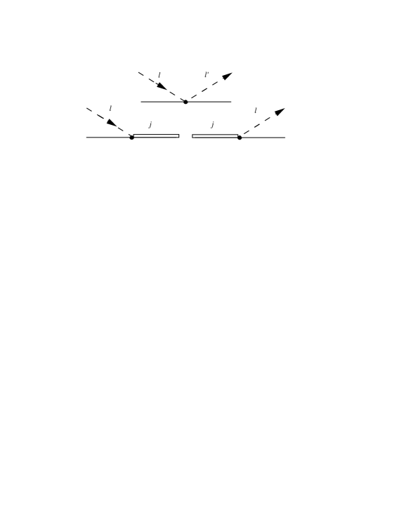
FIG. 1.: The vertices for the resonance and the contact interaction. The indices $l$ and $l^{\prime}$ stand for the meson type, the index $j$ refers to the resonances.

FIG. 2.: The four Riemann sheets for the pion and eta meson and the paths from one sheet to the next.

FIG. 3.: Pole movement in the $3^{rd}$ and the $2^{nd}$ ($4^{th}$) sheet (see text).

FIG. 4.: Argand diagram for the $\pi N$ partial wave $S_{11}$. Data from VPI [21].

FIG. 5.: Scattering cross sections for the partial wave $S_{11}$, calculated from the partial wave analysis by Arndt and Roper [21]. (—–) elastic cross section $\sigma_{s}$ for $\pi N\rightarrow\pi N$, (- - - - -) inelastic cross section $\sigma_{r}$. The data points are the cross sections for eta production [23].

FIG. 6.: Vertices for the two-pion system.

FIG. 7.: Riemann sheets when two-pion production is taken into account.

FIG. 8.: Real and imaginary part of the scattering amplitude $T_{0}$ ($S_{11}$-partial wave) for the model with $S_{11}(1535)$ (—) and without $S_{11}(1535)$ (-  - -).

FIG. 9.: The cross section for eta production in pion nucleon scattering. The solid and dashed lines show the model calculations with and without resonance $S_{11}$(1535). Experimental data are taken from Nefkens [23].

FIG. 10.: The pole positions on the Riemann sheets for our two models. ($\ast$) model with $S_{11}(1535)$, ($\Box$) model without $S_{11}(1535)$.

FIG. 11.: Vertices for the coupling of the photons to the nucleon and the mesons.

FIG. 12.: The total eta photoproduction cross section with resonance $S_{11}(1535)$ (—) and without $S_{11}(1535)$ (- - -).

FIG. 13.: Real- and imaginary part of the amplitude $E_{0+}$ with resonance $S_{11}(1535)$ (—) and without $S_{11}(1535)$ (- - -).

REFERENCES

- [1] M. Benmerrouche, N.C. Mukhopadhyay, J.F. Zhang, Phys. Rev. D 51 (1995) 3237
- [2] Ch. Sauermann, B.L. Friman, W. Nörenberg, Phys. Lett. B 341 (1995) 261
- [3] L. Tiator, C. Bennhold, B. Saghai, Nucl. Phys. A 580 (1994) 455
- [4] G. Höhler, A. Schulte, Newsletter No. 7 (1992) 76
- [5] G. Höhler, Karlsruhe preprint TTP97-36, to be published in Newsletter (1998)
- [6] N. Kaiser, T. Waas, W. Weise, Nuc. Phys. A 25 (1997) 297
- [7] T.D. Lee, Phys. Rev. 95 (1954) 1329
- [8] V. Glaser, G. Källén, Nucl. Phys. 2 (1956) 706
- [9] G. Källén, W. Pauli, Dan. mat. Fys. Medd. 30 No. 7 (1955)
- [10] G. Höhler, Z. Phys. 152 (1958) 546
- [11] S.S. Schweber, Relativistic Quantum Field Theory, Harper & Row, 1964
- [12] M. Lévy, Il Nouv. Cim. 13 (1959) 115
- [13] H.M. Nussenzveig, Causality and Dispersion Relations, Academic Press, 1972
- [14] A. Bohm, Quantum Mechanics, Foundations and Applications, Springer-Verlag, 1993
- [15] J. Denschlag, Diplomarbeit, KPH 19/94 Universität Mainz 1994
- [16] S.T. Ma, Rev. Mod. Phys. 25 (1953) 853
- [17] G. Höhler, F. Kaiser, R. Koch, E. Pietarinen, Handbook of Pion-Nucleon Scattering, Physics Data No. 12-1, Karlsruhe (1979)
- [18] G. Höhler, Landolt-Börnstein, Group 1, Volume 9, Springer-Verlag, 1983
- [19] R.E. Cutkosky et al., Phys. Rev. D 20 (1979) 2839
- [20] R.E. Cutkosky et al., Proc. 4th Conf. on Baryon Resonances in Toronto, ed. N. Isgur, (1980) p. 19
- [21] R.A. Arndt, L.D. Roper, Scattering Analysis Interactive Dial-In (SAID) Program, -N scattering solutions, said@clsaid.phys.vt.edu, Virginia Polytechnic Institute, Virginia, (1995)
- [22] L.D. Landau, E.M. Lifschitz, Lehrbuch der theoretischen Physik III, Quantenmechanik, Akademie- Verlag Berlin (1979), p. 593
- [23] M. Clajus, B.M.K. Nefkens, Pion Newsletter 7 (1992) 76
- [24] Y. Tomozawa, Nuovo Cim. 46A (1966) 707
- [25] S. Weinberg, Phys. Rev. Lett. 16 (1966) 879
- [26] M. Wilhelm, Dissertation, Bonn 1993
- [27] B. Krusche et al., Phys. Rev. Lett. 74 (1995) 3736