Damping Rates of Hot Giant Dipole Resonances

Abstract

The damping rate of hot giant dipole resonances (GDR) is investigated. Besides Landau damping we consider collisions and density fluctuations as contributions to the damping of GDR. Within the non-equilibrium Green’s function method we derive a non-Markovian kinetic equation. The linearization of the latter one leads to complex dispersion relations. The complex solution provides the centroid energy and the damping width of giant resonances. The experimental damping widths are the full width half maximum (FWHM) and can be reproduced by the full width of the structure function. Within simple finite size scaling we give a relation between the minimal interaction strength which is required for a collective oscillation and the clustersize. We investigate the damping of giant dipole resonances within a Skyrme type of interaction. Different collision integrals are compared with each other in order to incorporate correlations. The inclusion of a conserving relaxation time approximation allows to find the $T^{2}$-dependence of the damping rate with a temperature known from the Fermi-liquid theory. However, memory effects turn out to be essential for a proper treatment of the damping of collective modes. We derive a Landau like formula for the one–particle relaxation time similar to the damping of zero sound.

]

I Introduction

Giant resonances are high frequency, collective excitation modes of a nucleus. They can be identified as the collective motion in the nuclear volume and are found as a property of all nuclei. In particular in the last years the experimental and theoretical interest is focused to understand the width of such giant resonances [1, 2, 3, 4, 5, 6, 7, 8, 9, 10]. Although new experimental data are available at high excitation energy [11, 12] the theoretical description of the temperature dependence of damping rate is still a matter of discussion.

The theoretical treatment of giant resonances can be roughly characterized by two approaches. The first one considers the finite nucleus and solves the random phase approximation (RPA) equation by diagonalization of the Hamiltonian [13, 14]. In this approach the damping width can be extracted as an envelope of discrete excitation lines, sometimes called Landau fragmentation. However the introduction of the temperature remains difficult. The second class of approaches relies on the high density of states and consequently uses a continuous model, mostly the Fermi liquid theory [3, 7, 8, 9, 15, 16, 17]. Within this treatment, dispersion relations are derived whose solutions provide the energy and the width of collective excitations [8, 9, 17, 10].

The microscopic theory is mainly based on Vlasov kinetic equations [18, 19, 20]. The influence of correlations by particle-particle collisions is investigated using numerical solutions of Boltzmann–Uehling–Uhlenbeck (BUU)–type equations [21, 22]. To get more physical insight into these simulation results, collective models based on the scaling theory are developed [23]. It turns out that the non-Markovian kinetic equation is necessary to get realistic values for giant monopole resonances [2]. These collective models calculate the damping rate by an average procedure of the collision integral [24].

We follow another line. We will start from different kinetic equations and derive dispersion relations for the collective modes by linearization of the corresponding kinetic equation. Instead of collective averaging, we solve these dispersion relations and obtain directly the influence of correlations on the damping rate. We present in the paper different contributions to the damping of giant dipole resonances in a systematic way.

Let us shortly outline our theoretical approach to collective resonances. The collective density oscillations are determined via the time dependence of the one-particle distribution function $f(R,p,T)$ where the density reads $n(R,T)=\int\frac{d^{3}p}{(2\pi)^{3}}\,f(R,p,T)$. The one-particle distribution obeys the kinetic equation

$$\dot{f}(R,p,T) - \{{p^{2}\over 2m}+U(R,T)+U_{\rm ext}(R,T),f(R,p,T)\}$$ (1)

$$= I_{c}[f(R,p,T)]\,,$$ (2)

where $U$ is the mean-field potential and $I_{c}$ corresponds to the collisional term. The Poisson brackets are abbreviated as $\{a,b\}=\partial_{R}a\partial_{p}b-\partial_{p}a\partial_{R}b$. To get the linear response of the system to an external field $U_{ext}$ we linearize equation (2) around a quasi–equilibrium $f(R,p,T)=f^{0}(p)+\delta f(R,p,T)$ and get after Fourier transformation $T\rightarrow\omega$ and $R\rightarrow q$

$$i\omega\delta f(q,p,\omega)-i{pq\over m}\delta f(q,p,\omega)$$ (3)

$$+ i(U^{\prime}[n]\delta n(q,\omega)+U_{\rm ex})q\partial_{p}f_{0}(p)=I_{c}[\delta f(q,p,\omega)].$$ (4)

Integrating over $p$ the solution provides the polarization function $\Pi(q,\omega)$

$$\Pi(q,\omega)=\frac{\delta n(q,\omega)}{U_{ext}(q,\omega)}$$ (5)

with $\delta n(q,\omega)=\int\frac{d^{3}p}{(2\pi)^{3}}\,\delta f(q,p,\omega)$. In the RPA approximation which corresponds to the neglect of collisions we obtain

$$\Pi_{\rm RPA}(q,\omega)=\frac{\Pi^{0}(q,\omega)}{1-V_{0}\Pi^{0}(q,\omega)}\,$$ (6)

with the standard form of polarization function $\Pi^{0}$ (30) and $V_{0}=\partial_{n}U[n]$. The polarization function contains information about the collective excitation properties of nuclear matter. According to the denominator of (6) the relation to the dielectric function (DF) is given by

$$\epsilon(q,\omega)=1-V_{0}(n_{0})\Pi^{0}(q,\omega)\,.$$ (7)

For different collision integrals we will get different polarization functions. The complex zeros $\omega_{0}=\Omega-i\gamma$ of (7) determine the energy $\Omega$ and width $\gamma$ of the collective excitation. ¿From the DF one has the spectral function (structure function) via

$${\rm Im}\frac{1}{\epsilon(q,\omega)}=-\frac{{\rm Im}\epsilon(q,\omega)}{\big{[}{\rm Re}\epsilon(q,\omega)\big{]}^{2}+\big{[}{\rm Im}\epsilon(q,\omega)\big{]}^{2}}\,,$$ (8)

which is important because it’s structure reflects the collective excitations. Sum rules, e.g. [25]

$$\frac{1}{\pi V_{0}}\int\limits_{0}^{\infty}d\omega~{}\omega{\rm Im}\frac{1}{\epsilon(q,\omega)}=\frac{n_{0}q^{2}}{2m}\,$$ (9)

are an exact property of the spectral function.

The paper is organized as follows. In Sec.II we start with a generalized quantum kinetic equation which we rederived in appendix A using the Martin-Schwinger hierarchy for the real-time Green’s function. To include memory effects into the kinetic equation we use the generalized Kadanoff-Baym Ansatz and obtain a non-Markovian kinetic equation. In Sec.III we linearize these kinetic equations to get the DF for infinite hot nuclear matter in four different approximations: (Sec.III A) collisionless Vlasov equation, (Sec.III B) conserving relaxation time approximation (Mermin approximation), (Sec.III C) dynamical relaxation time approximation (reflecting memory effects) and (Sec. III D) the effect of density fluctuations on the potential. For these approximations we compare the damping rates and centroid energies of GDR which are the complex solution of the dispersion relation. In Sec.III E we discuss these results together with the FWHM of the structure function and with experimental data.

II Kinetic equation approach

Let us start from the kinetic equation in general form (A22) from appendix A

$$\left[\frac{\partial}{\partial T}+\frac{p}{m}\cdot\nabla_{R}\right]f_{W}(p,R,T)$$ (10)

$$+ \int dr\frac{dp^{\prime}}{(2\pi)^{3}}\,e^{i(p^{\prime}-p)\cdot r}f_{W}(p^{\prime},R,T)$$ (12)

$$\times\left[\Sigma_{H}(R+\frac{r}{2},T)-\Sigma_{H}(R-\frac{r}{2},T)\right]=I_{c},$$

$$I_{c}=\int\limits_{-\infty}^{0}d\tau\left[\left\{G^{>}(p,R,T-\frac{\tau}{2},\tau),\Sigma^{<}(p,R,T-\frac{\tau}{2},-\tau)\right\}\right.$$ (14)

$$\left.-\left\{G^{<}(p,R,T-\frac{\tau}{2},\tau),\Sigma^{>}(p,R,T-\frac{\tau}{2},-\tau)\right\}\right],$$

where the Wigner distribution function $f_{W}$ is connected to the correlation function $f_{W}(p,R,T)=G^{<}(p,R,T,\tau=0)$. Further $\{,\}$ is the anti-commutator of integrals over Wigner coordinates.
Neglecting the collision integral $I_{c}$ on the right hand side of (12) one obtains the collisionless quantum Vlasov equation [26]. This leads to the Lindhard polarization function (30).
Next, we will consider binary collisions and will use for the self-energy in (LABEL:allgI) the 1. Born approximation

$$\Sigma_{C}^{\stackrel{{\scriptstyle>}}{{<}}}(p,t-t^{\prime}) = \int\frac{d^{3}p^{\prime}d^{3}{\bar{p}}\,d^{3}{\bar{p}}^{\prime}}{(2\pi)^{9}}$$ (16)

$$\times W(pp^{\prime},{\bar{p}}{\bar{p}}^{\prime})(2\pi)^{3}\delta(p+p^{\prime}-{\bar{p}}-{\bar{p}}^{\prime})$$ (17)

$$\times G^{\stackrel{{\scriptstyle<}}{{>}}}(p^{\prime},t^{\prime}-t)G^{\stackrel{{\scriptstyle>}}{{<}}}({\bar{p}},t-t^{\prime})G^{\stackrel{{\scriptstyle>}}{{<}}}({\bar{p}}^{\prime},t-t^{\prime})\,,$$ (18)

where $W$ is the collision probability. We close equation (12) applying the generalized Kadanoff-Baym ansatz [27]

$$G^{<}(p,R,T,\tau)=e^{-\frac{i}{\hbar}\int\limits_{T-{\tau\over 2}}^{T+{\tau\over 2}}dt\epsilon(p,R,t)}f_{W}(p,R,T-\frac{|\tau|}{2})\,$$ (19)

which gives a connection between the correlation functions $G^{\stackrel{{\scriptstyle>}}{{<}}}$ and the Wigner distribution. The quasi-particle energy $\epsilon(p,R,T)$ in the quasi-particle picture is given by the solution of the dispersion relation

$$\epsilon=\frac{p^{2}}{2m}+U(R,T)+{\rm R}e\Sigma(p,\epsilon,R,T).$$ (20)

The resulting non-Markovian collision integral reads now

$$I_{m}(p_{1},T)=\int\limits_{0}^{\infty}d\tau\int\frac{d^{3}p_{2}d^{3}p_{3}}{(2\pi)^{6}}\,W(p_{1}p_{2},p_{3}p_{4})$$ (21)

$$\times \left[U^{+}(T-\tau,T)+U^{-}(T-\tau,T)\right]$$ (22)

$$\times \left[f_{3}(T-\tau)f_{4}(T-\tau)(1-f_{1}(T-\tau))(1-f_{2}(T-\tau))\right.$$ (23)

$$- \left.f_{1}(T-\tau)f_{2}(T-\tau)(1-f_{3}(T-\tau))(1-f_{4}(T-\tau))\right]$$ (24)

where $f_{i}(T)=f(p_{i},R,T)$ ($i=1,2,3,4$), $p_{4}=p_{1}+p_{2}-p_{3}$ and the full time dependent propagator $U^{\pm}$ is

$$U^{\pm}(T-\tau,T)=\exp[\pm i\int\limits_{T}^{T-\tau}dt^{\prime}\bigtriangleup\epsilon(t^{\prime})].$$ (26)

$\bigtriangleup\epsilon$ are the time dependent quasi-particle energies $\bigtriangleup\epsilon(t^{\prime})=\epsilon_{1}(t^{\prime})+\epsilon_{2}(t^{\prime})-\epsilon_{3}(t^{\prime})-\epsilon_{4}(t^{\prime})$. If memory effects are neglected, equation(LABEL:memorystoss1) becomes the usual Boltzmann or BUU collision integral $I_{B}$

$$I_{B} = \int\frac{d^{3}p_{2}d^{3}p_{3}}{(2\pi)^{6}}\,W(p_{1}p_{2},p_{3}p_{4})$$ (27)

$$\times \delta(\epsilon(p_{1})+\epsilon(p_{2})-\epsilon(p_{3})-\epsilon(p_{4})$$ (28)

$$\times \left[f_{3}f_{4}(1-f_{1})(1-f_{2})-f_{1}f_{2}(1-f_{3})(1-f_{4})\right]\,.$$ (29)

The Boltzmann collision integral is modified in (LABEL:memorystoss1) by a broadening of the delta distribution function of the energy conservation and an additional retardation in the center-of-mass times of the distribution functions $f_{i}=f(p_{i},R,T-\tau)$. The first effect is connected with phase decay or spectral properties and responsible for global energy conservation [28, 29]. The second effect gives rise to genuine memory effects. The formation of correlations at such short time scales are discussed in [29].

III Collective excitation and dielectric function

We now linearize the different derived kinetic equations and analyze their consequences to the damping of GDR. The standard RPA is first repeated in order to explain our analysis.

A Vlasov equation-collisionless Landau damping

The linearization of the quantum Vlasov equation (12) yields the RPA of the dielectric function which has the form of equation (7), but $\Pi_{0}$ is the (complex) Lindhard polarization function [30]

$$\Pi_{0}(\Omega,\gamma,q)=2\,\int_{c}\frac{d^{3}k}{(2\pi)^{3}}\frac{f(k)-f(k+q)}{E_{k}-E_{k+q}+(\Omega-i\gamma)+i\eta}$$ (30)

where $E_{k}=k^{2}/2m$ and $\eta$ is an infinitesimal small number. Spin degeneracy has been accounted for. $\Omega$ and $\gamma$ denote, respectively, the real part and the negative of the imaginary part of the frequency ($\omega=\Omega-i\gamma$). By consideration of a simplified Skyrme force [31]

$$\upsilon^{{}^{\prime}} = t_{0}(1+x_{0}\hat{P}_{\sigma})\delta(r_{1}-r_{2})+t_{3}\delta(r_{1}-r_{2})\delta(r_{2}-r_{3})\,,$$ (31)

one obtains a mean-field potential for the neutrons $U_{n}$ [32, 31]

$$U_{n}(R,T) = t_{0}\left\{\left(1+\frac{x_{0}}{2}\right)(n_{n}(R,T)+n_{p}(R,T))\right.$$ (33)

$$- \left.\left(x_{0}+\frac{1}{2}\right)n_{n}(R,T)\right\}$$ (34)

$$+ \frac{t_{3}}{4}\left\{(n_{n}(R,T)+n_{p}(R,T))^{2}-n_{n}^{2}(R,T)\right\}$$ (35)

and $U_{p}$ is given by an interchange of $n_{p}$ and $n_{n}$. ¿From (4) and (5) we can read off the effective particle-hole potential $V_{0}$ for isovector modes

$$U_{n}-U_{p} = 2V_{0}\left[\delta n_{n}-\delta n_{p}\right]$$ (36)

$$V_{0}(n_{0}) = -\frac{t_{0}}{2}\left(x_{0}+\frac{1}{2}\right)-\frac{t_{3}}{8}(n_{n}+n_{p})\,.$$ (37)

The parameter $t_{0}$, $t_{3}$ and $x_{0}$ were fitted to reproduce the binding energy ($E/A=-16$ MeV) at the saturation density ($n_{0}=0.17$ fm^-3) of nuclear matter. For the GDR the wave vector $q$ is estimated according to the formula [32, 33]

$$q=\frac{\pi}{2\,R}\,.$$ (38)

In this model neutrons and protons oscillate out of phase inside a sphere of the radius $R$ (=nuclear radius). Focusing our interest to the nucleus ²⁰⁸Pb (¹²⁰Sn) we use $q\approx 0.23$ fm^-1 ($q\approx 0.277$ fm^-1) with $R=6.7$ fm ($R=5.6$ fm).

The dispersion of collective excitation is now computed from the zeros of the complex dielectric function (DF), Eq. (7),

$$\mbox{Re}\,\epsilon(\Omega-i\gamma,q)+\mbox{Im}\,\epsilon(\Omega-i\gamma,q)=0$$ (39)

where $\gamma$ gives the Landau damping of the collective excitation. An approximate solution of this RPA dispersion relation is possible if the damping Im$\epsilon$ is small [34]. Then one can linearize the collective excitation spectrum

$${\rm Re}\epsilon(q,\Omega)+(\omega-\Omega+i\gamma)\partial_{\omega}{\rm Re}\epsilon(q,\Omega)+i{\rm Im}\epsilon(q,\Omega)=0$$ (40)

which leads to

$$\gamma={{\rm Im}\epsilon(q,\Omega)\over\partial_{\Omega}{\rm Re}\epsilon(q,\Omega)}$$ (42)

and $\Omega$ the solution of ${\rm Re}\epsilon(q,\Omega)=0$. This is, however only justified for small values of the damping $\gamma$. The correct procedure is to carry out the analytical continuation of the DF into the lower energy plane. Performing the integration one can express the DF (7) with (30) by the dimensionless variables $x=q/\sqrt{2mT}$, $z^{\ast}=\Omega/2T$ and $\xi=-\gamma/2T$ in the form

$$\epsilon(x,z^{\ast},\xi) = 1-\frac{V_{0}c}{2x}\int\limits_{C}dz\frac{F(z)}{z-z^{\ast}+i\xi}\quad\mbox{where}$$ (43)

$$F(z) = \ln\frac{1+\varsigma\exp-\left(z-\frac{x}{2}\right)^{2}}{1+\varsigma\exp-\left(z+\frac{x}{2}\right)^{2}}\,,$$ (44)

$c=\sqrt{2Tm^{3}}/\pi^{2}$ and $\varsigma=e^{\mu/T}$ denotes the fugacity. Following Landau’s contour integration [35] the result of the analytic continuation of the DF (43) with the pole $z_{0}=z^{\ast}-i\xi$ is

$$\epsilon^{c}(x,z^{\ast},\xi)=$$ (45)

$$1-\frac{V_{0}c}{2x}\left\{\begin{array}[]{ll}{\displaystyle\wp\int\limits_{-\infty}^{+\infty}dz\frac{F(z)}{z-z^{\ast}}+i\pi F(z^{\ast})}&\xi=0\\ {\displaystyle\int\limits_{-\infty}^{+\infty}dz\frac{F(z)}{z-z^{\ast}+i\xi}+i2\pi F(z^{\ast}-i\xi)}&\xi>0\\ {\displaystyle\int\limits_{-\infty}^{+\infty}dz\frac{F(z)}{z-z^{\ast}+i\xi}}&\xi<0.\end{array}\right.$$ (49)

(50)

The explicit expressions of the real and imaginary parts of the analytical continuation of the DF are given in appendix B. For complex values of $z$ there are also poles of the function $F(z)$ in (44) which require a separate investigation. They are located at

$$z_{n}=\pm\frac{x}{2}\pm\sqrt{\frac{\vartheta_{n}}{T}}\,,$$ (51)

where $\vartheta_{n}$ are the discrete fermionic Matsubara frequencies

$$\vartheta_{n}=\mu-i(2n+1)\pi T\,;\qquad n=0,\pm 1,\pm 2,...\,\,.$$ (52)

If these poles do not agree with the poles $z_{0}$ of the denominator of equation (43) there is no contribution to the integration due to the fact that Res$[F(z)/(z-z_{0});z_{n}]=0$. Because of the infinite residue the remaining case $z_{0}=z_{n}$ is found to be singular and will be discussed elsewhere.

Fig. 1 shows the zeros of the real and the imaginary part of the DF equation (50) in the complex plane at zero temperature (left hand side). The right hand side represents their position in the pair excitation spectrum which is bounded by the lines $\omega_{\pm}=q/2m(q\pm 2p_{F})$. For increasing wave vectors $q$ we have found three special cases:

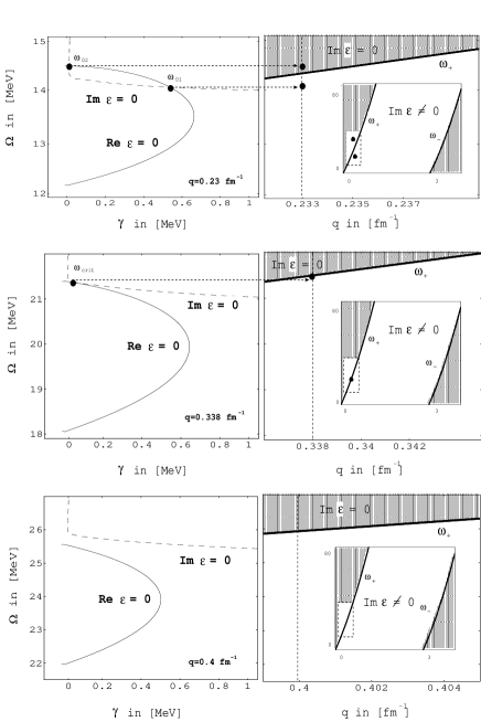
FIG. 1.: Zeros of the analytic continuation of the complex DF (Lindhard) for different wave vectors at $T=0$. LHS: collective excitations (GDR) in nuclear matter correspond to the crossing of the lines Re $\epsilon=0$ and Im $\epsilon=0$ (marked by thick dots). RHS: pair continuum Im $\epsilon\neq 0$ and undamped (marked) region Im $\epsilon=0,\gamma=0$ with $\omega_{\pm}=q/2m(q\pm 2p_{F})$.

Top (q=0.23 fm^-1): There are two collective excitations which correspond to the crossing points of the zeros of Re($\epsilon^{c}$) and Im($\epsilon^{c}$). Their resolution in the pair continuum (RHS) yields an undamped collective excitation $\omega_{02}$ which lies outside the pair continuum (marked region, Im$(\epsilon)=0$, $\gamma=0$). The collective excitation $\omega_{01}$ lies inside the pair continuum and is therefore damped (Im$(\epsilon)\neq 0$, $\gamma\neq 0$). From the DF one can now calculate the spectral function (8). In Fig. 2 one recognizes a $\delta$-shaped peak at the frequency of the undamped excitation $\omega_{02}$ and a broader peak corresponding to the damped collective excitation $\omega_{01}$.
Middle (q=0.338 fm^-1): There arises only one critical collective excitation $\omega_{crit}$ for a critical wave vector $q_{crit}$. The collective excitation $\omega_{crit}$ lies inside the pair continuum ($\omega_{crit}\approx\omega_{+}$) and is damped.
Bottom (q=0.4 fm^-1): Since there is no crossing of the zeros of the real part and the imaginary part of the DF, no collective excitation can occur.

FIG. 2.: Real part (solid line), imaginary part (dashed line) and spectral function (dotted line) of the Lindhard DF for the wave vector $q=0.23$ fm^-1 at $T=0$ corresponding to Fig. 1 (top).

In Fig. 3 we summarize the above results considering the entire dispersion of the collective excitation at $T=0$. We see that nuclear matter at zero temperature has a region where two collective modes are excited (Fig. 3 (A)). The mode $\Omega_{02}$ goes outside the pair continuum and is undamped, whereas the mode $\Omega_{01}$ propagates inside as a damped one.

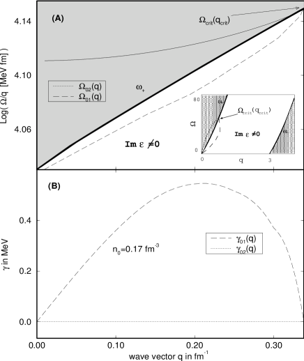
FIG. 3.: (A) Dispersion of the collective excitations at $T=0$ of Fig. 1 and their position in the pair continuum. The mode $\Omega_{02}(q)$ (dotted line) is undamped and $\Omega_{01}(q)$ (dashed line) is damped. The insert shows an enlarged view of the pair continuum where the marked region corresponds to the undamped region (Im=0). (B) Corresponding damping rates.

Beyond the coincidence of both modes into the critical point $\Omega_{crit}(q_{crit})\approx\omega_{+}(q_{crit})$ there are no further collective excitations. The related damping rates are shown in Fig. 3 (B). We observe that above a critical wave vector we cannot find collective excitations which represents a pure quantum effect. This critical wave vector $q_{crit}$ is determined by the used interaction $V_{0}$. Now we can link the minimal interaction required for collective oscillation with the mass number by equation (38). The relation between minimal interaction $V_{0_{crit}}$ and mass number $A_{crit}$ (wave vector $q_{crit}$) is plotted in Fig. 4. As a result we find the following fit

$$V_{0_{crit}}(A_{crit})=(a+\frac{b}{A_{crit}})\,\,\mbox{MeV fm}^{3}\,,$$ (53)

where $a=151.9$ and $b=2997.4$. The marked area Fig. 4 designates a region where no collective excitations exist. One sees that a certain interaction strength is necessary in order to have collective oscillations. The physical meaning is that for light nuclei with given interaction strength the sound velocity couples to the single particle motion more strongly. This fact is reflected in the critical wave vector, where the collective mode enters the pair continuum (cp. Fig. 3).

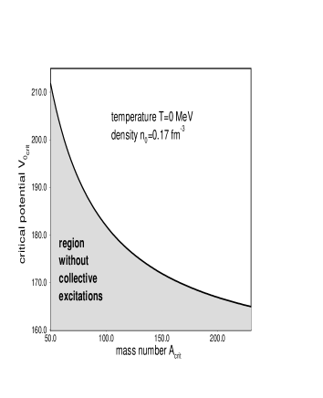
FIG. 4.: According to Fig. 1 (middle) calculated critical potentials $V_{0_{crit}}$ for critical wave vectors $q_{crit}$ which are connected with the mass number $A$ via (38). The marked area corresponds to a region where no collective excitations exist.

Since this model relies on the simple scaling law (38) the equation (53) can only be a qualitative estimation. For finite nuclei we expect different parameters $a$ and $b$.

Considering now nuclear matter for finite temperature we present in Fig. 5 the zeros of the real and imaginary part of the DF compared with the $T=0$ result. We find with growing temperatures a continuous deformation of the lines Re$(\epsilon^{c})=0$ and Im$(\epsilon^{c})=0$. The crossing points (black marked) correspond again to collective excitations and are always damped. We have additional zeros (light marked) in contrast to the zero temperature result. They correspond to the complex poles of equation (51) and can be identified as single particle excitations. Taking the entire dispersion relation for different temperatures (Fig. 6) we observe higher damping rates of the collective excitations as the temperature increases. This effect of temperature is also visible in the calculated spectral function (8) of Fig. 7.

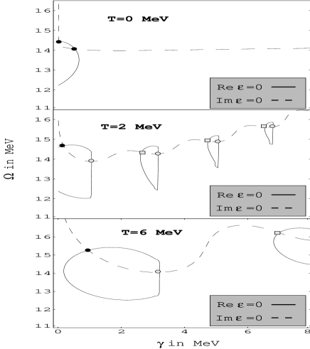
FIG. 5.: Collective excitations (thick dots) corresponding to the zeros of the analytic continuation of the complex DF (Lindhard) at different temperatures compared with the $T=0$ result (top or Fig. 1 (top)).

FIG. 6.: Collective excitations at $T=2$ MeV (solid line) and $T=6$ MeV (dot-dashed line) of Fig. 5. (A) Dispersion of the collective excitations, (B) damping rates.

Growing temperatures lead to a broadening of the peak and reaching a temperature of 6 MeV (solid line Fig. 7) only small collective effects remain observable. The corresponding centroid energy is increasing with higher temperatures. The further inclusion of correlations will lead to a decreasing of the centroid energy for higher temperatures, which has been demonstrated in [17, 31].

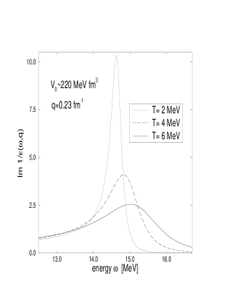
FIG. 7.: Imaginary part of the inverse Lindhard DF (spectral function) for different temperatures and the wave vector $q=0.23$ fm^-1. (This figure corresponds to the results of [31]).

In Fig. 8 we see now for the two nuclei ¹²⁰Sn and ²⁰⁸Pb (dotted lines) the calculated (Landau) damping rates of GDR over the nuclear temperature. These damping rates are compared and discussed with other approximation in the next sections.

B BUU equation-relaxation time approximation

In order to consider collisions as an additional damping effect of GDR we start first from (2) with the Markovian Boltzmann (BUU) collision integral (29) $I_{B}$.

Within the standard treatment [35] we linearize the collision integral around a homogeneous equilibrium distribution $f^{0}$

$$\delta f_{i}(p,R,T) = f_{i}(p,R,T)-f_{i}^{0}(\epsilon_{p})$$ (54)

$$\equiv \Phi_{i}(p,R,T)\frac{\partial}{\partial\epsilon_{p}}f_{i}^{0}$$ (55)

where $f_{i}^{0}$ should be first the global Fermi distribution. Later on we will use a local equilibrium distribution in order to ensure conservation laws. The linearized collision integral reads

$$I_{B} = \frac{1}{T}\int\frac{d^{3}p_{2}d^{3}p_{3}}{(2\pi)^{6}}\,W(p_{1}p_{2},p_{3}p_{4})\bigtriangleup\!\Phi\,\delta(\bigtriangleup\epsilon)$$ (56)

$$\times [f_{1}^{0}f_{2}^{0}(1-f_{3}^{0})(1-f_{4}^{0})]\,,$$ (57)

where $\bigtriangleup\epsilon=\epsilon_{1}+\epsilon_{2}-\epsilon_{3}-\epsilon_{4}$ and $\bigtriangleup\Phi=\Phi_{1}+\Phi_{2}-\Phi_{3}-\Phi_{4}$. Neglecting the backscattering terms $\Phi_{2}-\Phi_{3}-\Phi_{4}$ we obtain the relaxation time approximation

$$I_{B}=-\frac{f-f^{0}}{\tau(p_{1})}=-\frac{\delta f}{\tau(p_{1})}\,,$$ (58)

with

$$\frac{1}{\tau_{B}(p_{1})} = \int\frac{d^{3}p_{2}d^{3}p_{3}}{(2\pi)^{6}}\,W(12,34)\,\delta(\bigtriangleup\epsilon)$$ (59)

$$\times \frac{f_{2}^{0}(1-f_{3}^{0})(1-f_{4}^{0})}{1-f_{1}^{0}}.$$ (60)

Furthermore we will use a thermal averaged quantity. This procedure is introduced in appendix C and we get from (58)

$$\frac{1}{\tau_{B}} = \frac{1}{n_{D}}\int\frac{d^{3}p_{1}d^{3}p_{2}d^{3}p_{3}}{(2\pi)^{9}}\,W(p_{1}p_{2},p_{3}p_{4})\,\delta(\bigtriangleup\epsilon)$$ (61)

$$\times [f_{1}^{0}f_{2}^{0}(1-f_{3}^{0})(1-f_{4}^{0})]\,,$$ (62)

with $n_{D}=mp_{F}T/(2\pi^{2})$. For temperatures which are small compared to the Fermi energy we follow the well known methods of the Fermi liquid theory [36, 37] and get from (62)

$$\frac{1}{\tau_{B}}=\frac{2\pi m^{4}p_{f}}{n_{D}}\left<{W(\theta,\phi)\over\cos{\theta/2}}\right>\,I^{f}_{B}\,$$ (63)

where

$$\big{<}...\big{>}=\frac{1}{(2\pi)^{9}}\int\limits_{0}^{\pi}\,d\theta\sin\theta\int\limits_{0}^{2\pi}\,d\phi\int\limits_{0}^{2\pi}\,d\phi_{2}\,\frac{W(\theta,\phi)}{\cos{\theta/2}}\,.$$ (64)

The calculation of the Fermi integral $I^{f}_{B}$ is performed in appendix D with the result

$$I^{f}_{B}=\frac{2\pi^{2}}{3}T^{3}\,.$$ (65)

Using the collision probability in Born approximation we introduce the spin-isospin averaged cross section $\frac{d\sigma}{d\Omega}$

$$W(\theta,\phi)=2\pi\left|\frac{4\pi}{m}\right|^{2}\frac{d\sigma}{d\Omega}\,\,g$$ (66)

with the spin-isospin degeneracy $g=4$. Assuming a mean cross section $\frac{d\sigma}{d\Omega}\approx\frac{\sigma}{4\pi}$ we get finally

$$\frac{1}{\tau_{B}}=\frac{8}{3}T^{2}m\,\sigma\,,$$ (67)

where $\sigma$ is the nuclear cross section (for numerical calculation we use $\sigma=40$ mb as a spin-isospin averaged cross section of $\sigma_{nn}$, $\sigma_{pp}$ and $\sigma_{np}$ [38]).

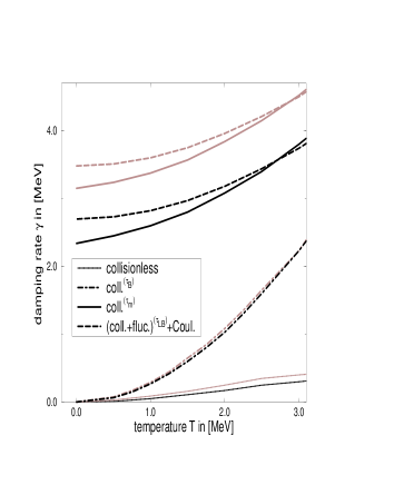
FIG. 8.: Theoretical damping rates of GDR for ¹²⁰Sn (grey) and ²⁰⁸Pb (black) as a function of the nuclear temperature $T$. They are the complex solution of the dispersion relation for different approximations: collisionless (Lindhard) DF (dotted line), Mermin DF (Boltzmann) (dot-dashed line), Mermin DF (memory) (solid line) and Mermin DF (density fluctuation+Coulomb interaction) (dashed line).

Based on this result one can use the relaxation time approximation to include collision effects into the DF. This leads to a pure replacement $\omega\rightarrow\omega+i/\tau$ in the collisionless Lindhard DF (30) and is known to violate the sum rule (9). Therefore we apply an extended approach using a conserving relaxation time approximation following Mermin [39]. The local equilibrium distribution $f^{0}$ is characterized by

$$f^{0}=\frac{1}{\exp[\beta(\epsilon_{p}-\mu-\delta\mu(R,t))]+1}\,,$$ (68)

where the local chemical potential $\delta\mu$ is determined by the density conservation resulting in $\delta\mu(q,\omega)=\frac{\delta n(q,\omega)}{\Pi^{0}(q,0)}$. The linearized kinetic equation (4) reads then

$$\left(\omega-\frac{q\cdot p}{m}\right)\delta f(p,q,w)=$$ (71)

$$\left[f^{0}(p-q/2)-f^{0}(p+q/2)\right]\,\delta V(q,\omega)$$

$$-\frac{1}{\tau_{B}}\left(\delta f(p,q,\omega)+\frac{\partial f^{0}(p)}{\partial\epsilon_{p}}\frac{\delta n(q,\omega)}{\Pi_{0}(q,0)}\right)$$

and the resulting (Mermin) DF is

$$\epsilon^{M}(q,\omega)=1+\frac{\displaystyle\left(1+\frac{i}{\omega\tau_{B}}\right)\left[\epsilon(q,\omega+i/\tau_{B})-1\right]}{\displaystyle 1+\left(\frac{i}{\omega\tau_{B}}\right)\frac{\left[\epsilon(q,\omega+i/\tau_{B})-1\right]}{\left[\epsilon(q,0)-1\right]}}\,.$$ (72)

Here $\epsilon$ is the collisionless Lindhard DF (to calculate the zeros of $\epsilon^{M}$ one has to use the analytical continuation of Lindhard DF equation (50)) and $\tau_{B}$ the relaxation time (67). Further conservation laws can be incorporated [40].

In Fig. 9 we compare the spectral functions computed with the Lindhard DF (dashed line) and Mermin DF (solid line), respectively. We observe an additional broadening beyond Landau damping in the width of the Mermin DF due to collision damping in this approximation. In comparison with Fig. 7 we see further that the centroid energy of Mermin result (solid line) is shifted to lower values with increasing temperature, while the centroid energy of the Lindhard result (dashed line) is shifted to higher values. The result for the damping rates $\gamma$ of the GDR of ¹²⁰Sn and ²⁰⁸Pb is shown in Fig. 8 (dot-dashed lines) which are determined by the zeros of the Mermin DF $\epsilon^{M}(\Omega,\gamma)=0$. The calculated damping rates in this approximation present an improvement compared to the collisionless results (dotted lines). We observe the typical $T^{2}$ behavior of the damping known from experimental data (Fig. 11) but we do not get any contribution at zero temperature. Now we shall employ a better approximation of collisions in the next section.

FIG. 9.: Spectral function (8) with the Lindhard DF (dashed line) compared with the Mermin DF for different relaxation times: Boltzmann relaxation time $\tau_{B}$ (solid line), dynamical (memory) dependent relaxation time $\tau_{m}$ (dot-dashed line).

C Non-Markovian equation-dynamical relaxation time

Next we investigate the kinetic equation with the collision integral (LABEL:memorystoss1) taking into account memory effects. The linearization of the collision term $I_{m}$ (LABEL:memorystoss1) can be performed in the same way as above with an additional linearization with respect to $U^{\pm}$. Expanding $U^{\pm}$ in (LABEL:memorystoss1) gives

$$\delta U^{\pm}(T-\tau,T)=U_{0}^{\mp}(\tau)\big{[}1\pm i\int\limits_{T}^{T-\tau}dt^{\prime}\,\bigtriangleup\delta\epsilon\big{]}\,,$$ (73)

where $\bigtriangleup\delta\epsilon=\bigtriangleup\epsilon(t^{\prime})-\bigtriangleup\frac{p^{2}}{2m}\,\,\mbox{and}\,\,U_{0}^{\pm}(\tau)=\exp(\pm i(\bigtriangleup\frac{p^{2}}{2m}\tau))$. The linearization of the collisional term (LABEL:memorystoss1) reads now

$$I_{m}(p_{1},T) = \int\limits_{0}^{\infty}d\tau\int\frac{d^{3}p_{2}d^{3}p_{3}}{(2\pi)^{6}}\,W(12,34)$$ (74)

$$\times \bigg{[}U_{0}^{+}(\tau)+U_{0}^{-}(\tau)(\delta F_{1}-\delta F_{2})$$ (76)

$$\bigg{.}+\delta U^{+}(T-\tau,T)-\delta U^{-}(T-\tau,T)\,F^{0}\bigg{]}$$

where

$$F^{0}= [f_{3}^{0}f_{4}^{0}(1-f_{1}^{0})(1-f_{2}^{0})-f_{1}^{0}f_{2}^{0}(1-f_{3}^{0})(1-f_{4}^{0})].$$ (77)

The calculation of $\delta F_{1}$ with the help of (55) results into

$$\delta F_{1} = f_{3}^{0}f_{4}^{0}(1-f_{1}^{0})(1-f_{2}^{0})$$ (79)

$$\times \frac{[f_{1}^{0}\Phi_{1}+f_{2}^{0}\Phi_{2}-(1-f_{3}^{0})\Phi_{3}-(1-f_{4}^{0})\Phi_{4}]}{T}$$ (80)

and $\delta F_{2}$ is obtained from equation (80) by interchanging $f\leftrightarrow(1-f)$. According to equation (4) we perform a Fourier transformation $T\rightarrow\omega$ of the linearized collision integral (76) with the result

$$I_{m}(p_{1},\omega) = \frac{1}{2}\int\frac{d^{3}p_{2}d^{3}p_{3}}{(2\pi)^{6}}\,W(12,34)$$ (81)

$$\times \left[D_{+}(\omega)\,\left(\delta F_{1}-\delta F_{2}\right)+\frac{D_{-}(\omega)}{\omega}\bigtriangleup\delta\epsilon\right]\,,$$ (82)

where $D_{\pm}(\omega)=\delta(\omega+\bigtriangleup\epsilon)\pm\delta(\omega-\bigtriangleup\epsilon)$. For $\delta\epsilon$ in (82) we obtain from the dispersion relation (20)

$$\delta\epsilon_{(}p_{i},R,T) = \frac{1}{1-\frac{\partial Re\Sigma(p_{i},R,T)}{\partial\Omega}|_{\Omega=\epsilon}}\Big{[}U^{\prime}(n_{0})\delta n(R,T)\Big{.}$$ (83)

$$+ \Big{.}\sum_{\bar{p}}\ \frac{\partial\Sigma(p_{i},R,T)}{\partial f(\bar{p},R,T)}\delta f(\bar{p},R,T)\Big{]}\,,$$ (84)

where $\delta n(R,T)=\sum_{\bar{p}}\delta f(\bar{p},R,T)$. In the following we neglect self-energy effects ($\Sigma=0$) and restrict our consideration to quasi-particle energies in mean-field approximation $\delta\epsilon(p_{i},R,T)=U^{\prime}(n_{0})\delta n(R,T)$ with $U^{\prime}=V_{0}$ from equation (37). Therefore we see that $\bigtriangleup\delta\epsilon=0$. This would be not the case for momentum dependent potentials.

One can now introduce a thermal averaged relaxation time $\tau_{m}$ analogous to (62)

$$\frac{1}{\tau_{m}(\omega)} = -\frac{1}{2n_{D}}\int\frac{d^{3}p_{1}d^{3}p_{2}d^{3}p_{3}}{(2\pi)^{9}}\,W(12,34)$$ (85)

$$\times \bigg{\{}D_{+}(\omega)\,f_{1}^{0}\bar{f_{1}^{0}}\left(\bar{f_{2}^{0}}f_{3}^{0}f_{4}^{0}-f_{2}^{0}\bar{f_{3}^{0}}\bar{f_{4}^{0}}\right)\bigg{\}}\,,$$ (86)

where $\bar{f}=(1-f)$ and $n_{D}$ is specified in appendix C. Comparing the Markovian result equation (62) with (86) we observe a replacement of the energy conserving factor $\delta(\epsilon)$ with $\delta(\omega+\bigtriangleup\epsilon)$ and $\delta(\omega-\bigtriangleup\epsilon)$. The energy $\hbar\omega$ of the collective excitations are now included into the energy conservation. We can interpret this effect as a coupling of the collective modes to the binary collisions. The collective boson is absorbed or emitted when two particles are colliding [38]. Restricting the relaxation time $\tau_{m}$ again to temperatures which are small compared to the Fermi energy we follow (62) and get from (86)

$$\frac{1}{\tau_{m}(\omega)}=\frac{2\pi m^{4}p_{f}}{n_{D}}\left<{W(\theta,\phi)\over\cos{\theta/2}}\right>\,I^{f}_{m}(\omega)\,$$ (87)

where the Fermi integral $I^{f}_{m}$ is done in appendix D with the result

$$I^{f}_{m}(\omega)=T^{3}\left[\frac{2}{3}\pi^{2}+\frac{1}{2}\left(\frac{\omega}{T}\right)^{2}\right].$$ (88)

The analytical expression for $\tau_{m}$ finally reads

$$\frac{1}{\tau_{m}(\omega)}=\frac{1}{\tau_{B}}\left[1+\frac{3}{4}\left(\frac{\omega}{\pi T}\right)^{2}\right]\,,$$ (89)

where $\tau_{B}$ is the relaxation time (67) which corresponds to the Markovian limit. The expression (89) for the relaxation time $\tau_{m}$ contains an additional (dynamical) contribution ($\sim\omega^{2}$). It guarantees that also at zero temperatures the collective mode can be considered as a self-propagating one which has a finite damping. We obtain a relaxation rate which is the Landau damping rate of zero sound [35] except the factor of 3 in front of the frequencies.

The form (89) is similar to the result Ayik derived in [38] for the collective damping rate. In contrast to this result we have here the single-particle relaxation time. As long as we have only momentum independent mean fields, the linearization of the mean field propagator does not reduce this to the standard Landau result as claimed in the errata of [38], instead the factor of 3 counts here (see comment after equation (84)).

One may argue that this factor 3 comes from the thermal averaging we employed here. We can repeat all calculations without thermal averaging (cp. appendix D 1) with the momentum in the relaxation time at the Fermi level. The resulting dynamical relaxation time reads then

$$\frac{1}{{\tilde{\tau}}_{m}(\omega)}=\frac{3}{4}\frac{1}{\tau_{B}}\left[1+\left(\frac{\omega}{\pi T}\right)^{2}\right]\,.$$ (90)

Compared with (89) one sees no factor $3$ appears in front of the frequency, however a factor $3/4$ in front of the relaxation time $1/\tau_{B}$. Therefore we obtain for $T=0$ the same frequency dependence in both cases. In other words the zero sound damping is not affected by averaging. The temperature dependence is slightly flatter without thermal averaging.

In the Mermin approximation $\epsilon^{M}$ of (72) we have to replace the static relaxation time $\tau_{B}$ with the dynamical one $\tau_{m}(\omega)$. Then we can again compute the damping rates $\gamma$ for the GDR of ¹²⁰Sn and ²⁰⁸Pb by searching for the zeros of the Mermin DF $\epsilon^{M}(\Omega,\gamma)=0$. The results are shown in Fig. 8 (solid lines). We observe a $T^{2}-$ dependence of the damping which is due to the low temperature expansion of the relaxation time $\tau_{m}$, but the temperature increase is too flat compared with the Boltzmann result (dot-dashed line). The inclusion of memory effects now induces a finite width at low temperatures. This reflects the fact that memory accounts for zero sound damping. Next we investigate the influence of density oscillations on the potential itself.

D Contribution of density fluctuations

As shown in [6] the contribution of density fluctuations can have an remarkable effect on the damping rate. The derivation of the kinetic equation including the density oscillations leads to Lenard-Balescu type of collision integrals [6] which have the same structure as (LABEL:memorystoss1) but with a dynamical potential

$$V^{2}(q)\rightarrow{V^{2}(q)\over|\epsilon(q,\epsilon_{1}-\epsilon_{1}^{\prime})|^{2}}\,,$$ (91)

replacing the static one. Here the DF renormalizes the potential. Then we can proceed as described above and linearize the collision integral, etc. This would lead to a rather involved integration. We simplify the treatment by assuming that the transfered momentum during a single collision is small. Since for small $q$ we have for the Lindhard DF

$$\lim\limits_{q\rightarrow 0}\epsilon(q,\omega)=1-\frac{c^{2}q^{2}}{\omega^{2}}+{\cal O}(q^{4})$$ (92)

with the free sound velocity $c^{2}=V_{0}n/m$, we get from (72)

$$\lim\limits_{q\rightarrow 0}\epsilon^{M}(q,\omega)=1-\frac{c^{2}q^{2}}{\omega(\omega+i/\tau)}\,.$$ (93)

Inspecting (86) we see that the frequency argument of (91) has to be taken at $\epsilon_{1}-\epsilon_{1}^{\prime}=q{2p_{2}+q\over 2m}\mp\omega\approx\mp\omega$ if we fix the final state of scattering as the state which matters for kinetic processes and use vanishing transfer momentum $q$. Further we observe that $|\epsilon(q,\omega)|=|\epsilon(q,-\omega)|$ such that we have a common factor in (86) in front of $D_{+}$ of $1/|\epsilon(q\rightarrow 0,\omega)|^{2}$. The further procedure is as above described. We expand for low temperatures and observe that for the angular averaging holds

$$\left<\frac{q^{2}}{\cos{\theta/2}}\right>=\left<\frac{2p_{F}\sin(\theta/2)\sin(\phi/2)}{\cos{\theta/2}}\right>\,.$$ (94)

Using (93) the resulting prefactor which renormalizes (86) reads

$${1\over\tau_{LB}(\omega)} = {1\over\tau_{m}(\omega)}\int\limits_{0}^{1}dx\,\left|\epsilon^{M}(2p_{F}x,\omega)\right|^{-2}$$ (95)

$$= {1\over\tau_{m}(\omega)}\int\limits_{0}^{1}dx\frac{1}{1-2{\rm Re}zx^{2}+|z|^{2}x^{4}}$$ (96)

with

$$z={4c^{2}p_{f}^{2}\over\omega(\omega+{i\over\tau})}$$ (97)

and the complex frequency $\omega=\Omega-i\gamma$. With tabulated integrals [41] we get from (96) finally an analytical expression

$${1\over\tau_{LB}(\Omega,\gamma)} = {1\over\tau_{m}(\Omega,\gamma)}\frac{k}{2\sin 2\alpha}$$ (98)

$$\times \bigg{[}\sin\alpha\,{\rm arctanh}(2k\cos{\alpha}+k^{2})$$ (100)

$$+\cos{\alpha}\Big{(}\arctan{\big{(}\frac{1-k^{2}}{2k\sin{\alpha}}\big{)}}+\frac{\pi}{2}\Big{)}\bigg{]}\,,$$

where $\alpha=\frac{1}{2}\arccos{({\rm Re}z/|z|^{2})}$ and $k=1/\sqrt{|z|}$. For our chosen situation and potential the prefactor (100) increases the damping rates only by $0.2$ MeV. However, we see that the renormalization of the potential by density fluctuations which are in turn determined by the linearization of the kinetic equation can lead in principal to a remarkable change in the dispersion relation if we come close to the instability line [6]. Our model potential (37) has no instability in the parameter range. The procedure here means that density fluctuations are caused by interactions or correlations, however these density fluctuations renormalize the potential, i.e. their cause. So we have a complicated feedback of correlations to the fluctuations and so forth.

1 Inclusion of Coulomb effects

We expect a more pronounced effect if long range interactions mediate collective oscillations. The Coulomb interaction leads to an additional contribution for the proton meanfield (35)

$$V^{C}=\frac{4\pi e^{2}}{q^{2}}n_{p}(q)\,,$$ (101)

so that the resulting dispersion relation will be a matrix equation [42]. As above, the damping rates $\gamma$ are again the complex solutions of this dispersion relation and plotted in Fig. 8 (dashed lines). For small temperatures we find an increasing of the damping rates compared with the rates of the memory dependent collision approximation (89) (solid lines). This comes from the fact that we have density fluctuations at zero temperature caused by the Coulomb interaction. For temperatures larger than $3$ MeV the binary collisions dominate and the behavior follows the memory collision approximation.

E Comparison with the Experiment

It is interesting to point out an advantage of the Mermin polarization function. Therefore we compute the power spectrum of the mode, i.e. the energy rate per time which is expended on the motion of the collective mode. This power spectrum is connected to the structure factor $S(q,\omega)=\sum\limits_{f}|<f|V_{0}|0>|^{2}\delta(\hbar\omega-E_{f}+E_{0})$ by

$$P(q,\omega)={2\pi\over\hbar}S(q,\omega)\hbar\omega$$ (102)

which is just Fermi’s Golden Rule. The structure factor itself is given by the dielectric function $S=V_{0}/\pi{\rm Im}\epsilon^{-1}$. Using (93) we arrive at an expression for the power spectrum of

$$P(q,\omega) = 2V_{0}\omega\;{\rm Im}{\omega(\omega+{i\over\tau})\over\omega(\omega+{i\over\tau})-{V_{0}nq^{2}\over m}}$$ (103)

$$= 2V_{0}\omega_{0}^{2}{{\omega^{2}\over\tau}\over(\omega^{2}-\omega_{0}^{2})^{2}+({\omega\over\tau})^{2}}$$ (104)

with $\omega_{0}^{2}=V_{0}nq^{2}/m$. The second line is derived with the assumption that $\tau$ is real, which is not true for dynamical relaxation times (memory effects). We rederive by this way just the classical Lorentz formula which describes the energy rate expended on the motion of a damped harmonic oscillator driven by the external force ${\stackrel{{\scriptstyle..}}{{x}}}+{\stackrel{{\scriptstyle.}}{{x}}}/\tau+\omega_{0}^{2}x=2V_{0}\omega_{0}^{2}\cos(\omega_{0}t)$ averaged over time.

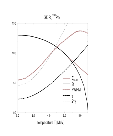
FIG. 10.: Temperature dependence of the centroid energy $E_{GDR}$ and of FWHM for GDR mode in ²⁰⁸Pb (grey lines) compared with the solution of the complex dispersion relation (39), ${\rm Re}\,\omega=\Omega$ and ${\rm Im}\,\omega=\gamma$ (dark lines), using the memory dependent relaxation time (89) in the Mermin DF (72).

Naturally that (104) leads to a Breit Wigner form near the resonance energy $\omega_{0}$ with the full width of half maximum (FWHM) of $\Gamma=1/\tau$

$$P(q,\omega) = V_{0}\omega_{0}^{2}{{\Gamma\over 2}\over(\omega-\omega_{0})^{2}+({\Gamma\over 2})^{2}}.$$ (105)

The damping rate in classical approximation (93) (long wavelength) is given as $\gamma=1/(2\tau)$. We recognize that the FWHM is just twice the damping rate $\Gamma=2\gamma$. This has been recently emphasized [8]. It has to be stressed that the experimental data are accessible by FWHM. To extract the FWHM from the structure function (8) we used the Mermin approximation $\epsilon^{M}$ (72) with the dynamical (memory) dependent relaxation time $\tau_{m}$ of (89).

In Fig. 10 we have plotted the temperature dependence of FWHM (grey-dashed line) of the structure function (cp. Fig. 9) and the corresponding centroid energy $E_{GDR}$ (grey-solid line) of the GDR mode in ²⁰⁸Pb together with real part $\Omega$ (dark-solid line) and imaginary part $\gamma$ (dark-dashed line) of the complex solution of the dispersion relation, respectively. We find an approximate relation $FWHM\approx 2\gamma$ (grey-dashed and thin dark-dashed lines) which holds in the temperature limit, where $FWHM<E_{GDR}$, as has been discussed in [8].

We emphasize that the centroid energy $E_{GDR}$ of the structure function agrees with the real part $\Omega$ of the complex solution of dispersion relation up to higher temperatures (thick-dark and thick-grey lines). The small deviation from the exact Breit Wigner form (105) is caused by the memory effects resulting in a frequency dependent dynamical relaxation time $\tau_{m}$ which is now complex.

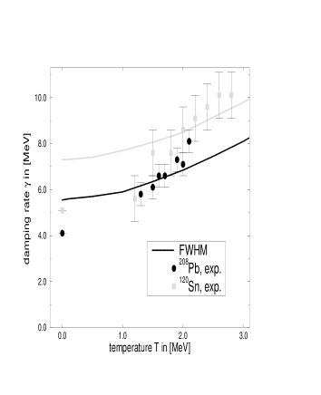
FIG. 11.: Experimental damping rates of GDR for ¹²⁰Sn and ²⁰⁸Pb (¹²⁰Sn from [11] and ²⁰⁸Pb from [12]) compared with the FWHM of the structure function as a function of the nuclear temperature $T$.

The FWHM is the observable which allows us to compare with the experimental data. In Fig. 11 we have plotted the FWHM of the GDR modes in ¹²⁰Sn (grey line) and ²⁰⁸Pb (dark line) as a function of temperature compared with experimental data. They coincide within theoretical limits if we consider that the experimental values are fits of a Breit Wigner form itself.

In Fig. 12 we compare different approximations calculated in this paper with experimental data versus mass number for $T=0$. In (A) we have plotted the centroid energy $\Omega=E_{GDR}$. We observe that the successive inclusion of collisions with the memory dependent relaxation time $\tau_{m}$ (89) (thin solid line), density fluctuations with the relaxation time $\tau_{LB}$ (100) (dashed line) as well as the inclusion of the Coulomb interaction (dotted and dot-dashed line) reproduces the experimental values (diamonds) increasingly for the mass numbers $80\leq\mbox{A}\leq 210$. The inclusion of only Coulomb effects (dotted line) slightly overestimates the data. This overestimate is compensated if we add the density fluctuations (dot-dashed line). The corresponding FWHM, which are shown to be roughly twice the imaginary parts $\gamma$ of the complex dispersion relations are plotted in Fig. 12(B). The inclusion of collisions brings the curve towards the experimental values. The improvement by inclusion of Coulomb effects and density fluctuations is small.

FIG. 12.: The experimental centroid energy $E_{GDR}$ (A) and the experimental data of the damping widths $\gamma$ (B) for GDR [43] vs mass number together with different approximations.

IV Summary

We have presented a systematic microscopic description of collective excitations in hot nuclear matter by a kinetic approach and computed damping rates of giant dipole resonances (GDR). We have rederived a generalized quantum kinetic equation employing the real-time Green functions technique. Within Hartree approximation one derives the collisionless Vlasov equation which in the linearized limit leads to the known Lindhard DF in RPA. Applying the complex integration method proposed by Landau we calculated the damping width (Landau damping) of GDR in different nuclei at finite temperatures.

The experimental data are calculated via the FWHM. Landau damping rates underestimate the experimental data of ¹²⁰Sn und ²⁰⁸Pb. Considering collisions in first Born approximation the (Markovian) kinetic equation is of Boltzmann or BUU type. Using a relaxation time approximation we have incorporated the collision effects into the DF which leads to the Mermin DF. The calculated damping rates of the GDR show a typical $T^{2}$-behavior but do not reproduce the experimental values yet. Only memory effects which are included into the collision term of the kinetic equation via retardation of the distribution function improve the theoretical damping rates. This non-Markovian relaxation time approximation leads to a dynamical relaxation time which differs from the Landau result of the damping of zero sound. Within the low temperature limit the theoretical damping rates of the GDR in ¹²⁰Sn und ²⁰⁸Pb are improved but the temperature increase is flatter than the experimental findings. A renormalization of the potential by density fluctuations increase the damping rates by $\approx 7\%$. These density fluctuations together with Coulomb effects reproduce the centroid energy for the mass numbers $80\leq\mbox{A}\leq 210$. If we neglect Coulomb interaction we underestimate the centroid energy for heavier elements.

We consider the solution of complex dispersion relations as the physical mode of collective excitation in the system. In contrast, the experimentally observed collective excitations are extracted from FWHM. The calculation of the width (FWHM) of the GDR modes, which is proportional to imaginary part of the inverse DF, leads to results which are comparable to the experiment. Memory effects change the shape of these structure functions compared to the usual Breit Wigner form. Since experimental data are fitted with the latter one, we cannot expect to reproduce the experimental data completely. Especially the temperature dependence of $\gamma$ as solution of the dispersion relation shows too small increase with temperature. This may be a hint that shape fluctuations become important [44]. In [45] it was stated that $\gamma$ increases linearly with temperature, caused by the coupling of surface modes. The incorporation of shape fluctuations will be considered in a forthcoming paper.

A Generalized kinetic equation

We shortly sketch the derivation of the general kinetic equation (LABEL:allgI). We use the dialect of the generalized Kadanoff and Baym formalism developed by Langreth and Wilkins [46] for the nonequilibrium (real-time) Green’s functions introduced by Kadanoff and Baym [26]. Considering a system of Fermions which interact via the potential $V$ we start with the Hamiltonian

$$\hat{H} = \int d^{3}r_{1}\Psi_{1}^{{\dagger}}\frac{\nabla^{2}}{2m}\Psi_{1}$$ (A1)

$$+ \frac{1}{2}\int d^{3}r_{1}d^{3}r_{2}\Psi_{1}^{\dagger}\Psi_{2}^{\dagger}V_{12}(r_{1}-r_{2})\Psi_{1}\Psi_{2},$$ (A2)

where the different numbers, i.e. $1=(r,t,s,...)$, denote the one-particle variables (space, time, spin,…). The annihilation and creation operators for Fermions obey the commutator relations

$$[\Psi_{1},\Psi_{2}]_{+}=0,\qquad[\Psi_{1},\Psi_{2}^{\dagger}]_{+}=\delta_{12}.$$ (A3)

The correlation functions are defined by different products of creation and annihilation operators in the Heisenberg picture

$$G^{>}(1,2)=\langle\Psi_{1}\Psi_{2}^{\dagger}\rangle,\qquad G^{<}(1,2)=\langle\Psi_{2}^{\dagger}\Psi_{1}\rangle.$$ (A4)

Here the $\langle...\rangle$ denotes the average value with the unknown quantum-statistical density operator $\rho$. The causal Green function is given with the Heaviside step function $\Theta$ by

$$G(1,2)=\Theta(t_{1}-t_{2})G^{>}(1,2)-\Theta(t_{2}-t_{1})G^{<}(1,2)$$ (A5)

It is furthermore useful to introduce the retarded and advanced Green functions according to

$$G^{R}(1,2)= - i\Theta(t_{1}-t_{2})[G^{>}(1,2)+G^{<}(1,2)]$$ (A6)

$$G^{A}(1,2)= i\Theta(t_{2}-t_{1})[G^{>}(1,2)+G^{<}(1,2)]\,.$$ (A7)

Using now the equation of motion of the creation and annihilation operators we can derive kinetic equations. Applying the equation of motion for the field operators in the Heisenberg picture one gets an equation of motion for the causal Green functions [26]

$$\left(i\frac{\partial}{\partial t_{1}}+\frac{\nabla_{1}^{2}}{2m}\right)G_{1}(1,1^{\prime})=$$ (A9)

$$\delta(1-1^{\prime})+\int d2\,V(1-2)G_{2}(12,1^{\prime}2^{+})\,.$$

In this so-called Martin-Schwinger hierarchy [26] the one-particle Green’s function couples to the two-particle one, the two-particle Green’s function couples to the three-particle one, etc. A formally closed equation for the one-particle equation can be reached with the introduction of the self-energy

$$\int\limits_{c}d{\bar{1}}\,\Sigma(1,{\bar{1}})G_{1}({\bar{1}},1^{\prime})=\int d2\,V(1-2)G_{2}(12,1^{\prime}2^{+})$$ (A10)

where the integration contour $c$ turns out to be chosen as Keldysh contour in order to meet the requirement of weakening of initial correlations

$$\lim\limits_{(t_{1}=t_{2}=t_{1}^{\prime}=t_{2}^{\prime})\rightarrow-\infty}G_{2}(12,1^{\prime}2^{\prime})$$ (A11)

$$= G(1,1^{\prime})G(2,2^{\prime})\pm G(1,2^{\prime})G(2,1^{\prime})$$ (A12)

which means that asymptotically the higher order correlations should be factorized for infinite past. One gets from (A9) and (A10) the Dyson equation

$$\left(i\frac{\partial}{\partial t_{1}}+\frac{\nabla_{1}^{2}}{2m}\right)G_{1}(1,1^{\prime})=\delta(1-1^{\prime})$$ (A13)

$$+ \int d{\bar{1}}\,\left(\Sigma(1,{\bar{1}})G_{1}({\bar{1}},1^{\prime})-\Sigma^{<}(1,{\bar{1}})G_{1}^{>}({\bar{1}},1^{\prime})\right).$$ (A14)

Writing (A14) into the more compact operator notation gives

$$G_{0}^{-1}G_{1}=1+\Sigma G_{1}\,,$$ (A15)

where $G_{0}^{-1}$ is the inverse of the Hartree–Fock Green function

$$G_{0}^{-1}(1,1^{\prime})=\left(i\frac{\partial}{\partial t_{1}}+\frac{\nabla_{1}^{2}}{2m}\right)\delta(1-1^{\prime})-\Sigma_{\rm HF}(1,1^{\prime})\,.$$ (A16)

We apply now the Langreth-Wilkins rules [46] onto the Dyson equation (A15), which describe the way to get the correlation functions (A5) and retarded functions (A7) from causal ones. We get the equation of motion

$$\left(G_{0}^{-1}-\Sigma^{R}\right)G^{\stackrel{{\scriptstyle>}}{{<}}}=\Sigma^{\stackrel{{\scriptstyle>}}{{<}}}G^{A}\,.$$ (A17)

Subtracting the adjoined equation the general kinetic equation reads [47]

$$-i\left(G_{0}^{-1}G^{<}-G^{<}G_{0}^{-1}\right)=$$ (A19)

$$i\left(G^{R}\Sigma^{<}-\Sigma^{<}G^{A}\right)-i\left(\Sigma^{R}G^{<}-G^{<}\Sigma^{A}\right)\,,$$

which was derived first by Kadanoff and Baym [26]. For the time diagonal case $t_{1}=t_{1^{\prime}}=t$ and using (A7) in (A19) we finally get

$$-i\left[G_{0}^{-1}(r_{1}t,r_{1^{\prime}}t),G^{<}(r_{1}t,r_{1^{\prime}}t)\right]=\int d^{3}{\bar{r}_{1}}\int\limits_{-\infty}^{t}d{\bar{t}_{1}}$$ (A20)

$$\bigg{(} G^{>}(r_{1}t,{\bar{1}})\Sigma^{<}({\bar{1}},r_{1^{\prime}}t)+\Sigma^{<}(r_{1}t,{\bar{1}})G^{>}({\bar{1}},r_{1^{\prime}}t)$$ (A21)

$$- G^{<}(r_{1}t,{\bar{1}})\Sigma^{>}({\bar{1}},r_{1^{\prime}}t)-\Sigma^{>}(r_{1}t,{\bar{1}})G^{<}({\bar{1}},r_{1^{\prime}}t)\bigg{)},$$ (A22)

which is the kinetic equation (12) and (LABEL:allgI), respectively.

B Expression of the dielectric function

In this appendix we give the explicit expressions of the real and imaginary parts of the analytical continuation of the complex dielectric function $\epsilon^{c}(q,\Omega,\gamma)$ in Eq. (50)

$${\rm Re}\,\epsilon^{c}(q,\Omega,\gamma)=\left\{\begin{array}[]{ll}\epsilon_{Re}(q,\Omega)~{},&\gamma=0\\ {\rm Re}\,\epsilon_{Re}(q,\Omega-i\gamma)&\\ -2\,{\rm Im}\,\epsilon_{Im}(q,\Omega-i\gamma)~{},&\gamma>0\\ {\rm Re}\,\epsilon_{Re}(q,\Omega-i\gamma)~{},&\gamma<0\\ \end{array}\right.$$ (B5)

$${\rm Im}\,\epsilon^{c}(q,\Omega,\gamma)=\left\{\begin{array}[]{ll}\epsilon_{Im}(q,\Omega)~{},&\gamma=0\\ {\rm Im}\,\epsilon_{Re}(q,\Omega-i\gamma)&\\ +2\,{\rm Re}\,\epsilon_{Im}(q,\Omega-i\gamma)~{},&\gamma>0\\ {\rm Im}\,\epsilon_{Re}(q,\Omega-i\gamma){}&\gamma<0~{},\\ \end{array}\right.$$ (B10)

where we redefined $\epsilon^{c}$ in terms of the retarded Lindhard DF $\epsilon(q,\omega)=\epsilon_{Re}+i\epsilon_{Im}$ (30). For nonzero temperature we find

$$\epsilon_{Re} = 1+\frac{V_{0}m}{\pi^{2}q}\int\limits_{0}^{\infty}dk\,k\,f_{F}(k)\,\Big{[}\phi(y_{+})-\phi(y_{-})\Big{]}\,,$$ (B11)

$$\epsilon_{Im} = -{V_{0}Tm^{2}\over\pi q}\ln\left|\frac{1+\exp^{\beta(\mu-(B^{\omega}_{-})^{2}/2m)}}{1+\exp^{\beta(\mu-(B^{\omega}_{+})^{2}/2m)}}\right|$$ (B12)

with $y_{\pm}=B^{\omega}_{\pm}/k$, $B^{\omega}_{\pm}=\omega m/q\pm q/2$, and $\phi(y)=\ln\left|(1-y)/(1+y)\right|$.

Considering now complex frequency $\omega=\Omega-i\gamma$ we find for $\epsilon_{Re}(q,\Omega,\gamma)={\rm Re}\,\epsilon_{Re}+{\rm Im}\,\epsilon_{Re}$

$${\rm Re}\,\epsilon_{Re} = 1-\frac{V_{0}m}{2\pi^{2}q}\int\limits_{0}^{\infty}dk\,k\,f_{F}(k)\,$$ (B13)

$$\times \left\{\ln\frac{(k^{2}-(B^{\Omega}_{+})^{2}-\kappa^{2})^{2}+(2k\kappa)^{2}}{\left[(k+(B^{\Omega}_{+})^{2}-\kappa^{2}\right]^{2}}\right.$$ (B15)

$$\left.-\ln\frac{(k^{2}-(B^{\Omega}_{-})^{2}-\kappa^{2})^{2}+(2k\kappa)^{2}}{\left[(k+B^{\Omega}_{-})^{2}-\kappa^{2}\right]^{2}}\right\}$$

and

$${\rm Im}\,\epsilon_{Re} = \frac{V_{0}m}{\pi^{2}q}\int\limits_{0}^{\infty}dk\,k\,f_{F}(k)\,$$ (B16)

$$\times \left[\arctan{\frac{2k\kappa}{(k^{2}-(B^{\Omega}_{+})^{2}-\kappa^{2})}}\right.$$ (B18)

$$\left.-\arctan{\frac{2k\kappa}{(k^{2}-(B^{\Omega}_{-})^{2}-\kappa^{2})}}\right]\,,$$

where $\kappa=\gamma m/q$.
The expressions of ${\rm Re}\,\epsilon_{Im}$ and ${\rm Im}\,\epsilon_{Im}$ are

$${\rm Re}\,\epsilon_{Im}=\frac{V_{0}mT}{2\pi q}\ln\left|\frac{\sigma_{c}^{2}+\sigma_{s}^{2}}{\sigma^{2}}\right|\,$$ (B19)

and

$${\rm Im}\,\epsilon_{Im}={V_{0}mT\over\pi q}\arctan\left(\frac{\sigma_{s}}{\sigma_{c}}\right)$$ (B20)

with

$$\sigma = 1+2a_{-}\cos(B^{\Omega}_{+}\kappa_{1})+a_{-}^{2}$$ (B21)

$$\sigma_{c} = 1+a_{+}\cos(B^{\Omega}_{-}\kappa_{1})+a_{-}\cos(B^{\Omega}_{+}\kappa_{1})+a_{+}a_{-}\cos(-\kappa_{1}q)$$ (B22)

$$\sigma_{s} = ~{}\,\,\quad a_{+}\sin(B^{\Omega}_{-}\kappa_{1})-a_{-}\sin(B^{\Omega}_{+}\kappa_{1})+a_{+}a_{-}\sin(-\kappa_{1}q).$$ (B23)

The coefficient $a_{\pm}$ is defined by

$$a_{\pm}=\exp(\mu/T)\exp\left[\frac{(-(B^{\Omega}_{\pm})^{2}+\kappa^{2})\kappa_{1}}{2\kappa}\right]$$ (B25)

where $\kappa_{1}=\gamma/Tq$. At zero temperature we used for the analytical continuation of the distribution function [48]

$$f_{F}(k)=\theta(k_{F}-|k|)$$ (B26)

with

$$f_{F}(k) = \lim_{\Delta\to 0}F_{\Delta}(k)~{},$$ (B27)

$$F_{\Delta}(k) = \frac{1}{\pi}\left\{\arctan\left[\frac{k+k_{F}}{\Delta}\right]-\arctan\left[\frac{k-k_{F}}{\Delta}\right]\right\}$$ (B28)

The calculation of ${\rm Re}\,\epsilon_{Re}$ (B13) and ${\rm Im}\,\epsilon_{Re}$ (B16) for complex frequencies will be done analogously. The imaginary part of $\epsilon_{Im}$ in Eq. (B12) vanishes if $\Delta$ goes to zero and can therefore be dropped.

C The thermal averaging

We define the thermal averaging by denoting that a function $A(\epsilon)$ should take its value onto the Fermi level for $T=0$

$$A(\epsilon_{f}) = \int d\epsilon\,\delta(\epsilon-\epsilon_{f})A(\epsilon)$$ (C1)

$$\approx \frac{1}{T}\int d\epsilon\,f^{0}(1-f^{0})A(\epsilon)$$ (C2)

$$= \frac{1}{n_{D}}\int\frac{d^{3}p}{(2\pi)^{3}}f^{0}(1-f^{0})A(\epsilon)$$ (C3)

with the density of state $n_{D}=mp_{f}T/(2\pi^{2})$ for low temperatures.

D Calculation of Collision integral

Performing the collision integral about Fermi functions in (63) with the dimensionless variables $x=(\epsilon-\mu)/T$ and $\lambda=\mu/T$ we get

$$I^{f}_{B}= T^{3} \int\limits^{\infty}_{-\lambda}dx_{1}\,dx_{2}\,dx_{3}\,dx_{4}\,\delta(\bigtriangleup x)f^{0}_{x_{1}}f^{0}_{x_{2}}\bar{f}^{0}_{x_{3}}\bar{f}^{0}_{x_{4}}$$ (D1)

where $f^{0}_{x}=(e^{x}+1)^{-1}$, $\bar{f_{x}^{0}}=1-f_{x}^{0}$ and $\bigtriangleup x=x_{1}+x_{2}-x_{3}-x_{4}$. The integral (D1) can be done exactly using the standard identity over Fermi functions [36] and we find

$$I_{B}^{f} = \frac{T^{3}}{2}\int\limits^{\infty}_{-\lambda}dx_{1}\,f^{0}_{x_{1}}\bar{f}^{0}_{x_{1}}(\pi^{2}+x_{1}^{2})$$ (D2)

$$= \frac{2\pi^{2}}{3}T^{3}\,.$$ (D3)

We perform the Fermi integral in (87) as above

$$I_{m}^{f}(\Omega)=\frac{I_{m}(\Omega)+I_{m}(-\Omega)}{2}$$ (D4)

and have for $I_{m}$

$$I_{m}(\pm\Omega) = T^{3}\int\limits^{\infty}_{-\lambda}dx_{1}\,dx_{2}\,dx_{3}\,dx_{4}\,\delta(\bigtriangleup x\pm\Omega)$$ (D6)

$$\times\left[f^{0}_{x_{1}}\bar{f}^{0}_{x_{1}}\left(\bar{f}^{0}_{x_{2}}f^{0}_{x_{3}}f^{0}_{x_{4}}+f^{0}_{x_{2}}\bar{f}^{0}_{x_{3}}\bar{f}^{0}_{x_{4}}\right)\right],$$

where $\Omega=\omega/T$. Writing (D6) in the form

$$I_{m}(\pm\Omega) = T^{3}\int\limits^{\infty}_{-\lambda}dx_{1}\,dx_{2}\,dx_{3}\,dx_{4}\,\delta(\bigtriangleup x\pm\Omega)$$ (D8)

$$\times\left[f^{0}_{x_{1}}f^{0}_{x_{2}}\bar{f}^{0}_{x_{3}}\bar{f}^{0}_{x_{4}}+{f^{0}_{x_{1}}}^{2}f^{0}_{x_{2}}\bar{f}^{0}_{x_{3}}\bar{f}^{0}_{x_{4}}\left({\rm e}^{\mp\Omega}-1\right)\right],$$

one gets for $\Omega\rightarrow 0$ the result (D3). Applying the standard identity[36] in (LABEL:memI2) we have

$$I_{m}(\pm\Omega) = \frac{T^{3}}{2}\int\limits_{-\lambda}^{\infty}dx_{1}\,\left[f_{x_{1}}^{0}+{f_{x_{1}}^{0}}^{2}\left({\rm e}^{\mp\Omega}-1\right)\right]$$ (D11)

$$\times\bar{f}^{0}_{x_{1}\pm\Omega}\left[\pi^{2}+(x_{1}\pm\Omega)^{2}\right]$$

$$= T^{3}\left(\frac{2}{3}\pi^{2}+\frac{\Omega}{2}^{2}\right)$$ (D12)

so that the final result for $I_{m}^{f}$ in (D4 ) reads

$$I_{m}^{f}(\omega) = T^{3}\left[\frac{2}{3}\pi^{2}+\frac{1}{2}\left(\frac{\omega}{T}\right)^{2}\right]$$ (D13)

$$= I_{B}^{f}\left[1+\frac{3}{4}\left(\frac{\omega}{\pi T}\right)^{2}\right]$$ (D14)

1 Without thermal averaging

Calculating the Fermi integral in (87) without the thermal averaging (app. C) we start from (D6) and get

$${\tilde{I}}_{m}(\pm\Omega) = T^{2}\int\limits^{\infty}_{-\lambda}dx_{2}\,dx_{3}\,dx_{4}\,\delta(\bigtriangleup x\pm\Omega)$$ (D16)

$$\times\left(\bar{f}^{0}_{x_{2}}f^{0}_{x_{3}}f^{0}_{x_{4}}+f^{0}_{x_{2}}\bar{f}^{0}_{x_{3}}\bar{f}^{0}_{x_{4}}\right).$$

Rewriting (D16) in the form

$${\tilde{I}}_{m}(\pm\Omega) = T^{2}\int\limits^{\infty}_{-\lambda}dx_{2}\,dx_{3}\,dx_{4}\,\delta(\bigtriangleup x\pm\Omega)$$ (D18)

$$\times f^{0}_{x_{2}}\bar{f}^{0}_{x_{3}}\bar{f}^{0}_{x_{4}}\left({\rm e}^{-x_{1}\mp\Omega}+1\right),$$

we apply the standard identity[36] and find for ${\tilde{I}}_{m}$

$${\tilde{I}}_{m}(x_{1},\pm\Omega) = \frac{T^{2}}{2\,\,}\bar{f}^{0}_{x_{1}\pm\Omega}\left[\pi^{2}+(x_{1}\pm\Omega)^{2}\right]\left({\rm e}^{-x_{1}\mp\Omega}+1\right).$$ (D19)

Since $\epsilon_{f}\approx\mu$ we have $x_{1}\rightarrow 0$ and get for ${\tilde{I}}^{f}_{M}$ (D4)

$${\tilde{I}}_{m}^{f}(\omega)=\frac{T^{2}\pi^{2}}{2}\left[1+\left(\frac{\omega}{\pi T}\right)^{2}\right].$$ (D21)

The resulting relaxation time ${\tilde{\tau}}_{m}$ reads finally

$$\frac{1}{{\tilde{\tau}}_{m}(\omega)}=\frac{3}{4}\frac{1}{\tau_{B}}\left[1+\left(\frac{\omega}{\pi T}\right)^{2}\right].$$ (D22)

REFERENCES

• [1] A. Smerzi, A. Bonasera, and M. Di Toro, Phys. Rev. C 44, 1713 (1991).
• [2] S. Ayik, M. Belkacem, and A. Bonasera, Phys. Rev. C 51, 611 (1995).
• [3] V. Kolomietz, V. Pluiko, and S. Shlomo, Phys. Rev. C 52, 2480 (1995).
• [4] M. Belkacem, S. Ayik, and A. Bonasera, Phys. Rev. C 52, 2499 (1995).
• [5] S. Suomijärvi et al., Phys. Rev. C 53, 2258 (1996).
• [6] K. Morawetz and M. Di Toro, Phys. Rev. C 54, 833 (1996).
• [7] V. Kolomietz, V. Plujko, and S. Shlomo, Phys. Rev. C 54, 3014 (1996).
• [8] M. Di Toro, V. Kolomietz, and A. Larionov, in proceedings of the Dubna conference on heavy ions (unpublished, Dubna, 1997).
• [9] V. Kondratyev and M. Di Toro, Phys. Rev. C 53, 2176 (1996).
• [10] E. Hernández, J. Navarro, A.Polls, and J. Ventura, Nucl. Phys. A 597, 1 (1996).
• [11] E. Ramkrishnan et al., Phys. Rev. Lett. 76, 2025 (1996).
• [12] E. Ramkrishnan et al., Nucl. Phys. A 549, 49 (1996).
• [13] J. Speth and J. Wambach, in International Review of Nuclear Physics (World Scientific, Singapore, 1991), Chap. 1.
• [14] V. Sokolov, I. Rotter, D. Savin, and M. Müller, Phys. Rev. C 56, 1031 (1997).
• [15] V. Abrosimov, M. Di Toro, and A. Smerzi, Z. Phys. A 347, 161 (1994).
• [16] S. Kamerdzhiev, Yad. Fiz. 9, 324 (1969).
• [17] V. Kolomietz, A. Larionov, and M. Di Toro, Nucl. Phys. A 613, 1 (1997).
• [18] D. Brink, Nucl. Phys. A 482, 205 (1986).
• [19] D. Brink, A. Dellafiore, and M. Di Toro, Nucl. Phys. A 456, 205 (1986).
• [20] A. Dellafiore and F. Matera, Nucl. Phys. A 460, 265 (1986).
• [21] V. Baran et al., Nucl. Phys. A 599, 29 (1996).
• [22] M. Colonna et al., Phys. Rev. B 307, 293 (1993).
• [23] P. Ring and P. Schuck, The Nuclear Many Body Problem (Springer, Berlin, 1982).
• [24] G. Bertsch, P. Bortignon, and R. Broglia, Rev. of Mod. Phys. 55, 287 (1983).
• [25] D. Pines and P. Nozières, The Theory of Quantum Liquids (Addison-Wesley, New York, 1968), Vol. 1.
• [26] L. Kadanoff and G. Baym, Quantum Statistical Mechanics (Addison-Wesley, New York, 1962).
• [27] P. Lipavský, V. Špička, and B. Velický, Phys. Rev. B 6, 3189 (1986).
• [28] K. Morawetz, Phys. Lett. A 199, 241 (1995).
• [29] K. Morawetz, V. Špička, and P. Lipavský, Phys. Rev. Lett. (1997), submitted.
• [30] J. Lindhard, Kgl. Danske Videnskab. Selskab. Mat. Fys. Medd. 28, 8 (1954).
• [31] F. Braghin and D. Vautherin, Phys. Lett. B 333, 289 (1994).
• [32] D. Vautherin and D. Brink, Phys. Rev. C 5, 626 (1972).
• [33] H. Steinwedel and J. Jensen, Z. f. Naturforschung 5, 413 (1950).
• [34] W.-D. Kraeft, D. Kremp, W. Ebeling, and G. Röpke, Quantum Statistics of Charged Particle Systems (Akademie-Verlag, Berlin, 1986).
• [35] E. Lifschitz and L. Pitajewski, Lehrbuch der Theoretischen Physik (Nauka, Moskau, 1978), Vol. 10.
• [36] H. Smith and H. Jensen, Transport Phenomena (Clarendon Press, Oxford, 1989).
• [37] G. Baym and C. Pethick, Landau Fermi-Liquid Theory (Wiley, New York, 1991).
• [38] S. Ayik and D. Boilley, Phys. Rev. B 276, 263 (1992), errata Phys. Lett. B 284, 482 (1992).
• [39] N. Mermin, Phys. Rev. B 1, 2362 (1970).
• [40] H. Heiselberg, C. J. Pethick, and D. G. Ravenhall, Ann. Phys. 223, 37 (1993).
• [41] I. Gradshteyn and I. Ryzhik, Table of Integrals, Series, and Products (Academic Press, San Diego, 1994).
• [42] K. Morawetz, R. Walke, U. Fuhrmann, and M. Di Toro, Phys. Rev. C (1997), submitted.
• [43] S. Dietrich and B. Berman, Nucl. Data Tabl. 38, 199 (1988).
• [44] P. Donati, N. Giovanardi, P. Bortignon, and R. Brogila, Phys. Lett. B 383, 15 (1996).
• [45] P. Donati, P. Bortignon, and R. Brogila, Z. Phys. A 354, 249 (1996).
• [46] D. Lengreth and G. Wilkins, Phys. Rev. B 34, 6933 (1972).
• [47] V. Špička and P. Lipavský, Phys. Rev. B 52, 14615 (1995).
• [48] M. Bonitz et al., Phys. Rev. E 49, 5535 (1994).