Exactly Solvable Models of Baryon Structure

Modelos Exactamente Solubles
de la Estructura Bariónica

ABSTRACT: We present a qualitative analysis of the gross features of baryon spectroscopy (masses and form factors) in terms of various exactly solvable models. It is shown that a collective model, in which baryon resonances are interpreted as rotations and vibrations of an oblate symmetric top, provides a good starting point for a more detailed quantitative study.

RESUMEN: Se presenta un análisis cualitativo de las propiedades generales de la espectroscopía bariónica (masas y factores de forma) en el contexto de varios modelos exactamente solubles. Se muestra que un modelo colectivo, en que se interpreta las resonancias bariónicas como rotaciones y vibraciones de un trompo oblato, provee un buen punto de partida para estudios más detaillados.

PACS: 03.65.Fd, 14.20.Gk, 13.40.Gp

1 Introduction

New dedicated experimental facilities (e.g. TJNAF, MAMI and ELSA) promise to produce new and more accurate data on the structure of the nucleon [1]. The nucleon is not an elementary particle, but it is generally viewed as a confined system of quarks interacting via gluon exchange. Effective models of the nucleon and its excited states (or baryon resonances) are based on three constituent parts that carry the internal degrees of freedom of spin, flavor and color, but differ in their treatment of radial (or orbital) excitations.

The purpose of this contribution is to discuss several exactly solvable models of baryon structure. Such models provide a set of closed analytic expressions for the mass spectrum, decay widths and selection rules that can be tested easily by experiment. We present a qualitative analysis of some salient features of baryon spectroscopy, such as the mass of the Roper resonance, the occurrence of linear Regge trajectories and the proton electric form factor, and discuss the merits and shortcomings of each scenario.

2 Algebraic models of the nucleon

We consider baryons to be built of three constituent parts. The internal degrees of freedom of these three parts are taken to be: flavor-triplet $u,d,s$ (for the light quark flavors), spin-doublet $S=1/2$, and color-triplet. The internal algebraic structure of the constituent parts consists of the usual spin-flavor ($sf$) and color ($c$) algebras

$${\cal G}_{i} = SU_{sf}(6)\otimes SU_{c}(3)~{}.$$ (1)

The relative motion of the three constituent parts can be described in terms of Jacobi coordinates, $\vec{\rho}$ and $\vec{\lambda}$, which in the case of three identical objects are

$$\vec{\rho} = \frac{1}{\sqrt{2}}(\vec{r}_{1}-\vec{r}_{2})~{},$$

$$\vec{\lambda} = \frac{1}{\sqrt{6}}(\vec{r}_{1}+\vec{r}_{2}-2\vec{r}_{3})~{}.$$ (2)

Here $\vec{r}_{1}$, $\vec{r}_{2}$ and $\vec{r}_{3}$ are the coordinates of the three constituents. Instead of a formulation in terms of coordinates and momenta we use the method of bosonic quantization, in which we introduce a dipole boson with $L^{P}=1^{-}$ for each independent relative coordinate, and an auxiliary scalar boson with $L^{P}=0^{+}$ [2]

$$b^{\dagger}_{\rho,m}~{},\;b^{\dagger}_{\lambda,m}~{},\;s^{\dagger}\hskip 28.45274pt(m=-1,0,1)~{}.$$ (3)

The scalar boson does not represent an independent degree of freedom, but is added under the restriction that the total number of bosons $N$ is conserved. This procedure leads to a compact spectrum generating algebra for the radial (or orbital) excitations

$${\cal G}_{r} = U(7)~{}.$$ (4)

For a system of interacting bosons the model space is spanned by the symmetric irreducible representation $[N]$ of $U(7)$. The value of $N$ determines the size of the model space.

For nonstrange $qqq$ baryons, the mass operator has to be invariant under the permuation group $S_{3}$, i.e. under the interchange of any of the three constituent parts. This poses an additional constraint on the allowed interaction terms. The eigenvalues and corresponding eigenvectors can be obtained exactly by diagonalization in an appropriate basis. The wave functions have, by construction, good angular momentum $L$, parity $P$, and permutation symmetry $t$. The three symmetry classes of the $S_{3}$ permutation group are characterized by the irreducible representations: $t=S$ for the one-dimensional symmetric representation, $t=A$ for the one-dimensional antisymmetric representation, and $t=M$ for the two-dimensional mixed symmetry representation.

The $S_{3}$ invariant $U(7)$ mass operator has a rich group structure. It is of general interest to study limiting situations, in which the mass spectrum can be obtained in closed analytic form, that is to say, in terms of a mass formula. These special cases correspond to dynamical symmetries, and arise whenever the mass operator can be written in terms of Casimir invariants of a chain of subgroups of $U(7)$ only. Under the restriction that the eigenstates have good angular momentum, parity and permutation symmetry, there are several possibilities. Here we consider the chains

$$U(7)\supset\left\{\begin{array}[]{l}U(6)\supset\left\{\begin{array}[]{l}{\cal SU}(3)\otimes SU(2)\supset{\cal SO}(3)\otimes SO(2)~{},\\ \mbox{}\\ SO(6)\supset SU(3)\otimes SO(2)\supset{\cal SO}(3)\otimes SO(2)~{},\end{array}\right.\\ \mbox{}\\ SO(7)\supset SO(6)\supset SU(3)\otimes SO(2)\supset{\cal SO}(3)\otimes SO(2)~{}.\end{array}\right.$$ (11)

The corresponding dynamical symmetries are referred to as the $U(6)\supset{\cal SU}(3)\otimes SU(2)$ limit, the $U(6)\supset SO(6)$ limit and the $SO(7)$ limit, respectively. These chains have the direct product group ${\cal SO}(3)\otimes SO(2)$ in common, where ${\cal SO}(3)$ is the angular momentum group and $SO(2)$ is related to the permutation symmetry [2, 3, 4].

The mass operator depends both on the spatial and the internal degrees of freedom. We first discuss the contribution from the spatial part, which is obtained by expanding the mass-squared operator in terms of the generators of $U(7)$ [2].

2.1 The (an)harmonic oscillator

The first chain corresponds to the problem of three particles in a common harmonic oscillator potential [3]. It separates the behavior in three-dimensional coordinate space determined by ${\cal SU}(3)\supset{\cal SO}(3)$, from that in the index space, given by $SU(2)\supset SO(2)$. The basis states are characterized by

$$\left|\begin{array}[]{ccccccccccc}U(7)&\supset&U(6)&\supset&{\cal SU}(3)&\otimes&SU(2)&\supset&{\cal SO}(3)&\otimes&SO(2)\\ N&,&n&,&&&F&,&L&,&M_{F}\end{array}\right>~{}.$$ (14)

The irreducible representations of ${\cal SU}(3)$ are determined by $n$ and $F$, and hence do not provide independent labels. The allowed values of the quantum numbers can be obtained from the branching rules. Table 1 shows the result for $N=2$. The mass spectrum in the $U(6)\supset{\cal SU}(3)\otimes SU(2)$ limit is given by

$$M^{2}(n,L,F,M_{F}) = M^{2}_{0}+\epsilon_{1}\,n+\epsilon_{2}\,n(n+5)$$ (15)

$$+\alpha\,F(F+2)+\kappa\,L(L+1)+\kappa^{\prime}M_{F}^{2}~{}.$$

In Fig. 1 we show the structure of the spectrum of an anharmonic oscillator with $U(6)$ symmetry. The levels are grouped into oscillator shells characterized by $n$. The ground state has $n=0$ and $L^{P}_{t}=0^{+}_{S}$. The one-phonon multiplet $n=1$ has two degenerate states with $L^{P}=1^{-}$ which belong to the two-dimensional representation $M$ of the permutation group, and the two-phonon multiplet $n=2$ consists of the states $L^{P}_{t}=2^{+}_{S}$, $2^{+}_{M}$, $1^{+}_{A}$, $0^{+}_{S}$ and $0^{+}_{M}$. The $\epsilon_{1}$ term gives rise to a harmonic spectrum, whereas the $\epsilon_{2}$ term introduces anharmonicities. The splitting within an oscillator shell is determined by the last three terms of Eq. (15). In Fig. 2 we show the splitting for the $n=2$ multiplet. The terms proportional to $\alpha$ and $\kappa^{\prime}$ separate the five states of the $n=2$ multiplet into two doublets with $L^{P}_{t}=2^{+}_{S}$, $0^{+}_{S}$ and $2^{+}_{M}$, $0^{+}_{M}$, respectively, and a $1^{+}_{A}$ singlet. Finally, the doublets can be split by adding the $L(L+1)$ term.

Another classification scheme for the six-dimensional oscillator is provided by the second group chain of Eq. (11). The reduction $U(6)\supset SO(6)\supset SU(3)\otimes SO(2)$ has been studied in detail in [5]. Here it is embedded in $U(7)$. The corresponding basis states are characterized by the labels

$$\left|\begin{array}[]{ccccccccccccc}U(7)&\supset&U(6)&\supset&SO(6)&\supset&SU(3)&\otimes&SO(2)&\supset&{\cal SO}(3)&\otimes&SO(2)\\ N&,&n&,&\sigma&,&&&M_{F}&,&L&&\end{array}\right>~{}.$$ (18)

The irreducible representations of $SU(3)$ are determined by $\sigma$ and $M_{F}$, and hence do not provide independent labels. Table 1 shows the classification scheme for $N=2$. The mass spectrum in the $U(6)\supset SO(6)$ limit is given by

$$M^{2}(n,\sigma,L,M_{F}) = M^{2}_{0}+\epsilon_{1}\,n+\epsilon_{2}\,n(n+5)$$ (19)

$$+\beta\,\sigma(\sigma+4)+\kappa\,L(L+1)+\kappa^{\prime}M_{F}^{2}~{}.$$

Also in this case the eigenstates are grouped into oscillator shells according to Fig. 1. However, the splitting within an oscillator shell is different from that in the $U(6)\supset{\cal SU}(3)\otimes SU(2)$ limit. Fig. 3 shows that the terms proportional to $\beta$ and $\kappa^{\prime}$ separate the five states of the $n=2$ multiplet into two doublets with $L^{P}_{t}=2^{+}_{S}$, $1^{+}_{A}$ and $2^{+}_{M}$, $0^{+}_{M}$, respectively, and a $0^{+}_{S}$ singlet. The difference between the two dynamical symmetries with $U(6)$ symmetry can be seen by comparing the position of the $0^{+}_{S}$ and $1^{+}_{A}$ states in Figs. 2 and 3.

2.2 The deformed oscillator

The two group chains associated with the $U(7)\supset U(6)$ reduction correspond to a six-dimensional anharmonic oscillator, for which the total number of oscillator quanta $n$ is a good quantum number. This is no longer the case for the third dynamical symmetry of Eq. (11), for which the basis states are labeled by

$$\left|\begin{array}[]{ccccccccccccc}U(7)&\supset&SO(7)&\supset&SO(6)&\supset&SU(3)&\otimes&SO(2)&\supset&{\cal SO}(3)&\otimes&SO(2)\\ N&,&\omega&,&\sigma&,&&&M_{F}&,&L&&\end{array}\right>~{}.$$ (22)

The classification scheme of the basis states for $N=2$ is given in Table 1. The $SO(7)$ limit corresponds to a deformed oscillator and its mass spectrum is given by

$$M^{2}(\omega,\sigma,L,M_{F}) = M^{2}_{0}+A\,(N-\omega)(N+\omega+5)$$ (23)

$$+\beta\,\sigma(\sigma+4)+\kappa\,L(L+1)+\kappa^{\prime}M_{F}^{2}~{}.$$

In Fig. 4 we show the mass spectrum of the deformed oscillator with $SO(7)$ symmetry. The states are now ordered in bands characterized by $\omega$, rather than in harmonic oscillator shells, as in the previous two examples. Although the size of the model space, and hence the total number of states, is the same as for the harmonic oscillator, the ordering and classification of the states is different. In the $U(6)$ limit, the states with $L^{P}_{t}=2^{+}_{S}$, $2^{+}_{M}$, $1^{+}_{A}$, $0^{+}_{S}$ and $0^{+}_{M}$ form the two-phonon multiplet, whereas in the $SO(7)$ limit the $0^{+}_{S}$ state is a vibrational excitation whose energy is determined by the value of $A$, and the $2^{+}_{S}$, $2^{+}_{M}$, $1^{+}_{A}$, $0^{+}_{M}$ states are rotations which belong to the ground state band with $\omega=N$ and whose excitation energies depend on $\beta$, $\kappa$ and $\kappa^{\prime}$.

2.3 The oblate symmetric top

Another interesting case, that does not correspond to a dynamical symmetry, is provided by the mass operator

$$M^{2} = \xi_{1}\,(R^{2}\,s^{\dagger}s^{\dagger}-b^{\dagger}_{\rho}\cdot b^{\dagger}_{\rho}-b^{\dagger}_{\lambda}\cdot b^{\dagger}_{\lambda})\,(R^{2}\,\tilde{s}\tilde{s}-\tilde{b}_{\rho}\cdot\tilde{b}_{\rho}-\tilde{b}_{\lambda}\cdot\tilde{b}_{\lambda})$$ (24)

$$+\xi_{2}\,\left[(b^{\dagger}_{\rho}\cdot b^{\dagger}_{\rho}-b^{\dagger}_{\lambda}\cdot b^{\dagger}_{\lambda})\,(\tilde{b}_{\rho}\cdot\tilde{b}_{\rho}-\tilde{b}_{\lambda}\cdot\tilde{b}_{\lambda})+4\,(b^{\dagger}_{\rho}\cdot b^{\dagger}_{\lambda})\,(\tilde{b}_{\lambda}\cdot\tilde{b}_{\rho})\right]~{},$$

with $\tilde{s}=s$ , $\tilde{p}_{\rho,m}=(-1)^{1-m}p_{\rho,-m}$ and $\tilde{p}_{\lambda,m}=(-1)^{1-m}p_{\lambda,-m}$ . For $R^{2}=0$ the mass operator of Eq. (24) has $U(7)\supset U(6)$ symmetry and corresponds to an anharmonic vibrator, whereas for $R^{2}=1$ and $\xi_{2}=0$ it has $U(7)\supset SO(7)$ symmetry and corresponds to a deformed oscillator. The general case with $R^{2}\neq 0$ and $\xi_{1}$, $\xi_{2}>0$ corresponds to an oblate symmetric top [2]. In a normal mode analysis the mass operator of Eq. (24) reduces to leading order in $N$ to a harmonic form, and its spectrum is given by [2]

$$M^{2}(v_{1},v_{2}) = \kappa_{1}\,v_{1}+\kappa_{2}\,v_{2}~{},$$ (25)

with $\kappa_{1}=\xi_{1}\,4NR^{2}$ and $\kappa_{2}=\xi_{2}\,4NR^{2}/(1+R^{2})$. Here $v_{1}$ and $v_{2}$ represent vibrational quantum numbers. In Fig. 5 we show a schematic spectrum of an oblate symmetric top. In anticipation of the application to the mass spectrum of nonstrange baryon resonances we have added a term linear in the angular momentum $L$. The spectrum consists of a series of vibrational excitations characterized by the labels $(v_{1},v_{2})$, and a tower of rotational excitations built on top of each vibration.

2.4 The hypercoulomb potential

Another exactly solvable model is provided by the hypercoulomb potential in six dimensions

$$H = \frac{1}{2\mu}\,(\vec{p}_{\rho}^{\,2}+\vec{p}_{\lambda}^{\,2})-\frac{\tau}{x}~{},$$ (26)

with $x=\sqrt{\vec{\rho}^{\,2}+\vec{\lambda}^{\,2}}$. This model can be solved in closed form by introducing hyperspherical coordinates [6, 7] or, equivalently, by using the properties of the noncompact dynamical group [8, 9]

$${\cal G}_{r} = SO(7,2)~{}.$$ (27)

The energy spectrum is given by

$$E(\omega) = -\frac{\tau^{2}\mu}{2(\omega+\frac{5}{2})^{2}}~{}.$$ (28)

The eigenstates are grouped into multiplets labeled by $\omega$. The degenerate states can be classified according to the symmetric representations of $SO(7)$ and its subgroups (see Table 1). In Fig. 6 we show the corresponding spectrum. It is important to note that, although the eigenvalues can be labeled by $\omega$, the eigenfunctions of Eq. (26) are not $SO(7)$ wave functions [9].

3 Mass spectrum

Here we consider the nonstrange baryon resonances belonging to the nucleon (isospin $I=1/2$) and the delta (isospin $I=3/2$) family. The full algebraic structure is obtained by combining the spatial part ${\cal G}_{r}$ of Eq. (4) or (27) with the internal spin-flavor-color part ${\cal G}_{i}$ of Eq. (1)

$${\cal G} = {\cal G}_{r}\otimes SU_{sf}(6)\otimes SU_{c}(3)~{}.$$ (29)

The spatial part of the baryon wave function has to be combined with the spin-flavor and color part, in such a way that the total wave function is antisymmetric. Since the color part of the wave function is antisymmetric (color singlet), the remaining part (spatial plus spin-flavor) has to be symmetric. For nonstrange resonances which have three identical constituent parts this means that the symmetry of the spatial wave function under $S_{3}$ is the same as that of the spin-flavor part. Therefore, one can use the representations of either $S_{3}$ or $SU_{sf}(6)$ to label the states. The subsequent decomposition of representations of $SU_{sf}(6)$ into those of $SU_{f}(3)\otimes SU_{s}(2)$ is the standard one

$$S\;\leftrightarrow\;[56] \supset {}^{2}8\,\oplus\,^{4}10~{},$$

$$M\;\leftrightarrow\;[70] \supset {}^{2}8\,\oplus\,^{4}8\,\oplus\,^{2}10\,\oplus\,^{2}1~{},$$

$$A\;\leftrightarrow\;[20] \supset {}^{2}8\,\oplus\,^{4}1~{}.$$ (30)

The representations of the spin-flavor groups $SU_{sf}(6)$, $SU_{f}(3)$ and $SU_{s}(2)$ are denoted by their dimensions. The total baryon wave function is expressed as

$$\left|\Psi\right> = \left|\,{}^{2S+1}\mbox{dim}\{SU_{f}(3)\}_{J}\,[\mbox{dim}\{SU_{sf}(6)\},L^{P}]\,\right>~{},$$ (31)

where $S$ and $J$ are the spin and total angular momentum $\vec{J}=\vec{L}+\vec{S}$. As an example, the nucleon wave function is given by

$$\left|\Psi\right> = \left|\,{}^{2}8_{1/2}\,[56,0^{+}]\,\right>~{}.$$ (32)

In the previous section we have discussed four exactly solvable models to describe the radial (or orbital) excitations of baryons. The mass spectrum of nonstrange baryons is characterized by the lowlying N(1440) resonance with $J^{P}=1/2^{+}$ (the socalled Roper resonance), whose mass is smaller than that of the first excited negative parity resonances, and the occurrence of linear Regge trajectories. These two features make an interpretation in terms of the harmonic vibrator, the deformed oscillator or the hypercoulomb potential model difficult.

The Roper resonance has the same quantum numbers as the nucleon of Eq. (32), but is associated with the first excited $L_{t}^{P}=0^{+}_{S}$ state. In the harmonic oscillator the first excited $L_{t}^{P}=0^{+}_{S}$ state belongs to the $n=2$ positive parity multiplet which lies above the first excited negative parity state with $n=1$ (see Fig. 1), whereas the data shows the opposite. In the hypercoulomb potential model the Roper resonance occurs at the same mass as the negative parity resonances, whereas in the deformed oscillator and the oblate top the Roper resonance is a vibrational excitation whose mass is independent of that of the negative parity states which are interpreted as rotational excitations.

Furthermore, the data show that the mass-squared of the resonances depends linearly on the orbital angular momentum $M^{2}\propto L$. The resonances belonging to such a Regge trajectory have the same quantum numbers with the exception of $L$. In Fig. 7 we show the trajectories for the positive parity resonances $|^{2}8_{J=L+1/2}\,[56,L^{+}]\rangle$ with $L=0,2,4$ and for the negative parity resonances $|^{2}8_{J=L+1/2}\,[70,L^{-}]\rangle$ with $L=1,3,5$. The splitting of the rotational states in the harmonic oscillator and the hypercoulomb potential model is hard to reconcile with linear Regge trajectories.

In the oblate top and the deformed oscillator it is straightforward to reproduce the relative mass of the Roper resonance and the occurrence of linear Regge trajectories. The main difference between these two models is the interpretation of the first excited $0^{+}_{M}$ state. In the deformed oscillator it is a rotational excitation that belongs to the ground band $(\omega=N)$, whereas in the oblate top it is a fundamental vibration. In Tables 2 and 3 we present an analysis of nonstrange baryon resonances in terms of vibrations and rotations of an oblate symmetric top. A simultaneous fit of the 25 well-established (3 and 4 star) nucleon and delta resonances of [10] gives a r.m.s. deviation of 39 MeV [2]. The 1 and 2 star resonances are not very well established experimentally. For some of these resonances we have indicated several possible assignments. In addition to the resonances presented in Tables 2 and 3 there are many more states calculated than have been observed so far, especially in the nucleon sector. The lowest socalled ‘missing’ resonances correspond to the unnatural parity states with $L^{P}=1^{+}$, $2^{-}$, which are decoupled both in electromagnetic and strong decays, and hence very difficult to observe.

4 Form factors

In addition to the mass spectrum it is important to investigate the decay channels of baryon resonances. The generic form of a (partial) decay width is

$$\Gamma = \rho\,\chi\,|F(k)|^{2}~{},$$ (33)

where $\rho$ is a phase space factor, $\chi$ contains the spin-flavor dependence and $F(k)$ is the geometric form factor that depends on the momentum transfer. All models discussed in this article have the same spin-flavor structure, but differ in the treatment of the radial excitations, and hence in the geometric form factor. Helicity asymmetries of baryon resonances $(|A_{1/2}|^{2}-|A_{3/2}|^{2})/(|A_{1/2}|^{2}+|A_{3/2}|^{2})$ only depend on the spin-flavor part and cannot be used to distinguish between the different models of baryon structure, since in the ratio of the difference and the sum of the helicity $1/2$ and $3/2$ amplitudes the phase space factor and the geometric form factor cancel.

However, electromagnetic form factors which can be measured in electroproduction of baryon resonances do provide a good test of various models of baryon structure. Here we use the proton electric form factor $G_{E}^{p}$ as an example. It can be shown that $G_{E}^{p}$ is proportional to the radial matrix element

$$G_{E}^{p}(k) = \langle\Psi_{p}|\,\mbox{e}^{-ik\sqrt{\frac{2}{3}}\lambda_{z}}\,|\Psi_{p}\rangle~{}.$$ (34)

In the hypercoulomb potential model this matrix element can be derived in closed form either in coordinate space [6, 7] or algebraically [9]

$$G_{E}^{p}(k)\;=\;\frac{1}{(1+k^{2}b^{2})^{7/2}}\;=\;1-\frac{7}{2}k^{2}b^{2}+\ldots~{},$$ (35)

with $b^{2}=25/24\tau^{2}\mu^{2}$. In principle, the coefficient $b$ can be determined by the charge radius of the proton $b^{2}=\langle r^{2}\rangle_{p}/21$.

In $U(7)$ the Jacobi coordinate $\lambda_{z}$ is expressed in terms of algebraic operators as [2, 11]

$$\sqrt{\frac{2}{3}}\lambda_{z} \rightarrow \beta\,\hat{D}_{\lambda,z}/X_{D}~{},$$ (36)

where the dipole operator $\hat{D}_{\lambda,m}=(b^{\dagger}_{\lambda}\tilde{s}-s^{\dagger}\tilde{b}_{\lambda})^{(1)}_{m}$ is a generator of $U(7)$ that transforms as a vector under rotations, is even under time reversal, and transforms under permutations as the Jacobi coordinate $\lambda_{m}$. The coefficient $X_{D}$ is a normalization factor and $\beta$ represents the scale of the coordinate. The proton radial wave function $|\Psi_{p}\rangle$ depends on the model that is used to describe the orbital excitations. For the three limiting cases of $U(7)$ that were discussed above we obtain

$$G_{E}^{p}(k) = \left\{\begin{array}[]{ll}\mbox{e}^{-k^{2}\beta^{2}/6}\;=\;1-k^{2}\beta^{2}/6+\ldots&\mbox{Harmonic oscillator}\\ \mbox{}\\ 4J_{2}(k\beta\sqrt{2})/k^{2}\beta^{2}\;=\;1-k^{2}\beta^{2}/6+\ldots&\mbox{Deformed oscillator}\\ \mbox{}\\ j_{0}(k\beta)\;=\;1-k^{2}\beta^{2}/6+\ldots&\mbox{Oblate top}\end{array}\right.$$ (42)

The scale parameter $\beta$ can be determined by the charge radius of the proton $\beta^{2}=\langle r^{2}\rangle_{p}$.

In a collective model of baryons the nucleon has a specified distribution of charge and magnetization [2, 11]

$$g(\beta)=\beta^{2}\,\mbox{e}^{-\beta/a}/2a^{3}~{},$$ (43)

where $a$ is a scale parameter. The ansatz of Eq. (43) was made to obtain the dipole form for the oblate top

$$G_{E}^{p}(k)\;=\;\int_{0}^{\infty}d\beta\,g(\beta)\,j_{0}(k\beta)\;=\;\frac{1}{(1+k^{2}a^{2})^{2}}\;=\;1-2k^{2}a^{2}+\ldots~{}.$$ (44)

For the deformed oscillator we find

$$G_{E}^{p}(k)\;=\;\frac{(\sqrt{1+2k^{2}a^{2}}-1)^{2}}{k^{4}a^{4}\sqrt{1+2k^{2}a^{2}}}\;=\;1-2k^{2}a^{2}+\ldots~{}.$$ (45)

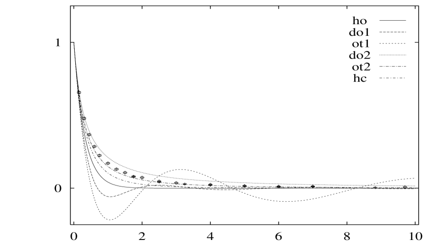
Figure 8: Comparison between the experimental and calculated proton electric form factor $G_{E}^{p}$ as a function of $Q^{2}=k^{2}$. The curves labeled by ho, do1, ot1, do2, ot2 and hc are calculated with Eqs. (42), (45), (44) and (35), respectively. The experimental data are taken from [12] and [13].

Again the scale parameter $a$ can be determined by the charge radius of the proton $a^{2}=\langle r^{2}\rangle_{p}/12$. For small momentum transfer the behavior of the proton electric form factor is the same for all cases considered, since it is determined by the proton charge radius. However, for large momentum transfer the behavior is very different. Eq. (42) shows that, whereas for the harmonic oscillator $G_{E}^{p}$ drops exponentially, for the deformed oscillator and the oblate top it exhibits an oscillatory behavior. In a collective model of the nucleon introduced in Eq. (43) the proton electric form factor drops as $k^{-4}$ for the oblate top (by construction), and as $k^{-3}$ for the deformed oscillator. For the hypercoulomb potential model $G_{E}^{p}$ drops as $k^{-7}$. In Fig. 8 we show a comparison with the data. In Fig. 9 we have divided $G_{E}^{p}$ by a dipole form factor $1/(1+k^{2}/0.71)^{2}$ to show more clearly the differences between the various model calculations.

5 Summary and conclusions

In summary, we have presented a qualitative analysis of the mass spectrum and form factors of nonstrange baryons in the context of several exactly solvable models. These models share a common spin-flavor structure, but differ in their treatment of radial excitations. We first discussed a $U(7)$ interacting boson model of baryons for the spatial degrees of freedom [2]. It was shown that this model unifies various exactly solvable models and, as such, provides a general framework to study the properties of baryon resonances in a transparent and systematic way. For nonstrange baryon resonances it contains the (an)harmonic vibrator, the deformed oscillator and the oblate symmetric top as special cases. Another solvable model that we have considered is the hypercoulomb potential model. Although the hypercoulomb potential is not confining, it is nevertheless worthwhile to examine its main features. Confining terms can added later and studied numerically [7].

It was shown that a collective model, in which baryon resonances are interpreted as rotations and vibrations of an oblate symmetric top, can account for the mass of the Roper resonance, the linear Regge trajectories and the proton electric form factor. Hence this scenario provides a good starting point for a more detailed quantitative study of baryons.

Table 1: Classification scheme of the basis states in (a) the $U(6)\supset{\cal SU}(3)\otimes SU(2)$ limit, (b) the $U(6)\supset SO(6)$ limit, and (c) the $SO(7)$ limit. The number of bosons is $N=2$.

(a)				(b)				(c)
$n$	$F$	$M_{F}$	$L^{P}_{t}$	$n$	$\sigma$	$M_{F}$	$L^{P}_{t}$	$\omega$	$\sigma$	$M_{F}$	$L^{P}_{t}$
0	0	0	$0^{+}_{S}$	0	0	0	$0^{+}_{S}$	2	0	0	$0^{+}_{S}$
1	1	$\pm 1$	$1^{-}_{M}$	1	1	$\pm 1$	$1^{-}_{M}$		1	$\pm 1$	$1^{-}_{M}$
2	2	$\pm 2$	$0^{+}_{M},2^{+}_{M}$	2	2	$\pm 2$	$0^{+}_{M},2^{+}_{M}$		2	$\pm 2$	$0^{+}_{M},2^{+}_{M}$
		0	$0^{+}_{S},2^{+}_{S}$			0	$1^{+}_{A},2^{+}_{S}$			0	$1^{+}_{A},2^{+}_{S}$
	0	0	$1^{+}_{A}$		0	0	$0^{+}_{S}$	0	0	0	$0^{+}_{S}$

Table 2: Mass spectrum of nucleon resonances in the oblate top model. The masses are given in MeV.

Baryon	Status	State	($v_{1},v_{2}$)	$M_{\mbox{calc}}$
N$(939)P_{11}$	****	${}^{2}8_{1/2}[56,0^{+}]$	(0,0)	939
N$(1440)P_{11}$	****	${}^{2}8_{1/2}[56,0^{+}]$	(1,0)	1440
N$(1520)D_{13}$	****	${}^{2}8_{3/2}[70,1^{-}]$	(0,0)	1566
N$(1535)S_{11}$	****	${}^{2}8_{1/2}[70,1^{-}]$	(0,0)	1566
N$(1650)S_{11}$	****	${}^{4}8_{1/2}[70,1^{-}]$	(0,0)	1680
N$(1675)D_{15}$	****	${}^{4}8_{5/2}[70,1^{-}]$	(0,0)	1680
N$(1680)F_{15}$	****	${}^{2}8_{5/2}[56,2^{+}]$	(0,0)	1735
N$(1700)D_{13}$	***	${}^{4}8_{3/2}[70,1^{-}]$	(0,0)	1680
N$(1710)P_{11}$	***	${}^{2}8_{1/2}[70,0^{+}]$	(0,1)	1710
N$(1720)P_{13}$	****	${}^{2}8_{3/2}[56,2^{+}]$	(0,0)	1735
N$(1900)P_{13}$	**	${}^{2}8_{3/2}[70,2^{+}]$	(0,0)	1875
N$(1990)F_{17}$	**	${}^{4}8_{7/2}[70,2^{+}]$	(0,0)	1972
N$(2000)F_{15}$	**	${}^{2}8_{5/2}[70,2^{+}]$	(0,0)	1875
		${}^{4}8_{5/2}[70,2^{+}]$	(0,0)	1972
N$(2080)D_{13}$	**	${}^{2}8_{3/2}[70,1^{-}]$	(1,0)	1909
		${}^{4}8_{3/2}[70,1^{-}]$	(1,0)	2004
N$(2090)S_{11}$	*	${}^{2}8_{1/2}[70,1^{-}]$	(1,0)	1909
		${}^{4}8_{1/2}[70,1^{-}]$	(1,0)	2004
N$(2100)P_{11}$	*	${}^{2}8_{1/2}[70,1^{+}]$	(0,1)	1997
		${}^{4}8_{1/2}[70,1^{+}]$	(0,1)	2088
N$(2190)G_{17}$	****	${}^{2}8_{7/2}[70,3^{-}]$	(0,0)	2140
N$(2200)D_{15}$	**	${}^{2}8_{5/2}[70,3^{-}]$	(0,0)	2140
		${}^{4}8_{5/2}[70,3^{-}]$	(0,0)	2225
N$(2220)H_{19}$	****	${}^{2}8_{9/2}[56,4^{+}]$	(0,0)	2267
N$(2250)G_{19}$	****	${}^{4}8_{9/2}[70,3^{-}]$	(0,0)	2225
N$(2600)I_{1,11}$	***	${}^{2}8_{11/2}[70,5^{-}]$	(0,0)	2590
N$(2700)K_{1,13}$	**	${}^{2}8_{13/2}[56,6^{+}]$	(0,0)	2695

Table 3: Mass spectrum of delta resonances in the oblate top model. The masses are given in MeV.

Baryon	Status	State	($v_{1},v_{2}$)	$M_{\mbox{calc}}$
$\Delta(1232)P_{33}$	****	${}^{4}10_{3/2}[56,0^{+}]$	(0,0)	1232
$\Delta(1600)P_{33}$	***	${}^{4}10_{3/2}[56,0^{+}]$	(1,0)	1646
$\Delta(1620)S_{31}$	****	${}^{2}10_{1/2}[70,1^{-}]$	(0,0)	1649
$\Delta(1700)D_{33}$	****	${}^{2}10_{3/2}[70,1^{-}]$	(0,0)	1649
$\Delta(1750)P_{31}$	*	${}^{2}10_{1/2}[70,0^{+}]$	(0,1)	1786
$\Delta(1900)S_{31}$	***	${}^{2}10_{1/2}[70,1^{-}]$	(1,0)	1977
$\Delta(1905)F_{35}$	****	${}^{4}10_{5/2}[56,2^{+}]$	(0,0)	1909
$\Delta(1910)P_{31}$	****	${}^{4}10_{1/2}[56,2^{+}]$	(0,0)	1909
$\Delta(1920)P_{33}$	***	${}^{4}10_{3/2}[56,2^{+}]$	(0,0)	1909
$\Delta(1930)D_{35}$	***	${}^{2}10_{5/2}[70,2^{-}]$	(0,0)	1945
$\Delta(1940)D_{33}$	*	${}^{2}10_{3/2}[70,2^{-}]$	(0,0)	1945
$\Delta(1950)F_{37}$	****	${}^{4}10_{7/2}[56,2^{+}]$	(0,0)	1909
$\Delta(2000)F_{35}$	**	${}^{2}10_{5/2}[70,2^{+}]$	(0,0)	1945
$\Delta(2150)S_{31}$	*	${}^{4}10_{1/2}[56,1^{-}]$	(0,1)	2029
		${}^{2}10_{1/2}[70,1^{-}]$	(0,1)	2062
$\Delta(2200)G_{37}$	*	${}^{2}10_{7/2}[70,3^{-}]$	(0,0)	2201
$\Delta(2300)H_{39}$	**	${}^{4}10_{9/2}[56,4^{+}]$	(0,0)	2403
		${}^{2}10_{9/2}[70,4^{+}]$	(0,0)	2431
$\Delta(2350)D_{35}$	*	${}^{4}10_{5/2}[56,3^{-}]$	(0,0)	2170
		${}^{2}10_{5/2}[70,3^{-}]$	(0,0)	2201
$\Delta(2390)F_{37}$	*	${}^{2}10_{7/2}[70,3^{+}]$	(0,0)	2201
		${}^{4}10_{7/2}[56,4^{+}]$	(0,0)	2403
		${}^{2}10_{7/2}[70,4^{+}]$	(0,0)	2431
$\Delta(2400)G_{39}$	**	${}^{2}10_{9/2}[70,4^{-}]$	(0,0)	2431
$\Delta(2420)H_{3,11}$	****	${}^{4}10_{11/2}[56,4^{+}]$	(0,0)	2403
$\Delta(2750)I_{3,13}$	**	${}^{4}10_{13/2}[56,5^{-}]$	(0,0)	2615
		${}^{2}10_{13/2}[70,6^{-}]$	(0,0)	2835
$\Delta(2950)K_{3,15}$	**	${}^{4}10_{15/2}[56,6^{+}]$	(0,0)	2811

Figure 1: Schematic spectrum of an anharmonic oscillator with $U(6)$ symmetry. The masses are calculated using Eq. (15) with $\epsilon_{1}>0$, $\epsilon_{2}>0$ and $\alpha=\kappa=\kappa^{\prime}=0$. The number of bosons is $N=2$.

Figure 2: Splitting of the $n=2$ multiplet in the $U(6)\supset{\cal SU}(3)\otimes SU(2)$ limit. The masses are calculated using Eq. (15) by successively adding the terms with $\alpha<0$, $\kappa^{\prime}<0$ and $\kappa>0$.

Figure 3: Splitting of the $n=2$ multiplet in the $U(6)\supset SO(6)$ limit. The masses are calculated using Eq. (19) by successively adding the terms with $\beta>0$, $\kappa^{\prime}<0$ and $\kappa>0$.

Figure 4: Schematic spectrum of a deformed oscillator with $SO(7)$ symmetry. The masses are calculated using Eq. (23) with $A>0$, $\beta>0$ and $\kappa=\kappa^{\prime}=0$. The number of bosons is $N=2$.

Figure 5: Schematic spectrum of an oblate symmetric top. The masses are calculated using Eq. (25) with $\kappa_{1}>0$, $\kappa_{2}>0$ and an additional term linear in $L$.

Figure 6: Schematic spectrum of a hypercoulomb potential model. The masses are calculated using Eq. (28) with $\tau^{2}\mu>0$.

Figure 7: Regge trajectories for the positive parity resonances $|^{2}8_{J=L+1/2}\,[56,L^{+}]\rangle$ with $L=0,2,4$ and the negative parity resonances $|^{2}8_{J=L+1/2}\,[70,L^{-}]\rangle$ with $L=1,3,5$. The lines represent the result for the oblate symmetric top.

Figure 9: As Fig. 8, but divided by the dipole form factor $1/(1+k^{2}/0.71)^{2}$.

References

- [1] See e.g. Proceedings of the ‘Fourth CEBAF/INT Workshop on N* Physics’, Eds. T.-S.H. Lee and W. Roberts, World Scientific, 1997.
- [2] R. Bijker, F. Iachello and A. Leviatan, Ann. Phys. (N.Y.) 236, 69 (1994).
- [3] P. Kramer and M. Moshinsky, Nucl. Phys. 82, 241 (1966).
- [4] K.C. Bowler, P.J. Corvi, A.J.G. Hey, P.D. Jarvis and R.C. King, Phys. Rev. D 24, 197 (1981); A.J.G. Hey and R.L. Kelley, Phys. Rep. 96, 71 (1983).
- [5] E. Chacón, O. Castaños and A. Frank, J. Math. Phys. 25, 1442 (1984).
- [6] J. Leal Ferreira and P. Leal Ferreira, Lett. Nuovo Cimento 3, 43 (1970).
- [7] E. Santopinto, F. Iachello and M.M. Giannini, Z. Phys. A, in press.
- [8] A.O. Barut and Y. Kitagawara, J. Phys. A: Math. Gen. 14, 2581 (1981).
- [9] R. Bijker, F. Iachello and E. Santopinto, submitted, preprint nucl-th/9801051.
- [10] Particle Data Group, Phys. Rev. D 54, 1 (1996).
- [11] R. Bijker, F. Iachello and A. Leviatan, Phys. Rev. C 54, 1935 (1996).
- [12] R.C. Walker et al., Phys. Rev. D 49, 5671 (1994).
- [13] L. Andivahis et al., Phys. Rev. D 50, 5491 (1994).