Center-of-mass corrections revisited:
a many-body expansion approach

Abstract

A many-body expansion for the computation of the charge form factor in the center-of-mass system is proposed. For convergence testing purposes, we apply our formalism to the case of the harmonic oscillator shell model, where an exact solution exists. We also work out the details of the calculation involving realistic nuclear wave functions. Results obtained for the Argonne $v$18 two-nucleon and Urbana-IX three-nucleon interactions are reported. No corrections due to the meson-exchange charge density are taken into account.

2

I Introduction

One of the successes of the shell-model picture has been the ability to calculate self-consistent densities for nuclear ground states that not only reproduce experimental binding energies but also experimental charge radii of these nuclei and generally nuclear charge densities. The excellent agreement or remaining discrepancies have been a cornerstone for advancing our understanding of the nuclear wave function. In particular, the ability to predict both, heavy and light nuclei, is taken as a confirmation of the quality of the effective nuclear interaction used in the calculations. For that reason it is useful to examine the accuracy with which the nuclear densities can be calculated.

For the proper description of the scattering process one assumes a nuclear wave function that factorizes into a nuclear center-of-mass wave function, which is taken to be a plane wave, and an intrinsic wave function of coordinates relative to the center-of-mass. The difficulty lies in the ansatz of the wave function as a Slater determinant. Such a wave function generally does not factorize into a center-of mass wave function and a wave function for the nucleus relative to its center-of-mass. Furthermore, for the cases where it factorizes, the center-of-mass wave function is not a plane wave. While this is negligible for heavy nuclei, it is a significant correction for nuclei like ¹⁶O.

This problem has been known for a long time. It can be solved exactly for a single Slater determinant of harmonic oscillator single-particle wave functions. In that case it has been shown that the wave function factorizes with a center-of-mass wave function being a Gaussian. This allows us to calculate the form factor, i.e. the Fourier transform of the density, in the form

$$F_{sd}(q)\ =\ e^{-\,\frac{1}{4}b^{2}q^{2}/A}\ F_{int}(q)$$ (1)

given in terms of the harmonic oscillator length parameter $b$. The calculation usually gives the form factor of the one-body density labeled $F_{sd}(q)$ whereas the experiment requires the form factor with respect to the center-of-mass, labeled $F_{int}(q)$. Because of this exact result it has been customary to apply such a correction also in cases where the single particle wave functions are not harmonic oscillator wave functions and where the presence of correlations has been substituted by an effective interaction.

An alternate way to deal with this is to calculate directly the form factor in the center-of-mass system. This way the operator can be written as a series of one-body, two-body, …, to A-body terms. In this paper we first compare such an expansion with the exact result, for the case where such a result is available. We then apply the same expansion to a realistic wave function of ¹⁶O [1] and compare it to the corrections implied by equation (1). This nuclear wave function was derived for ¹⁶O using correlations of the form $exp({\mathbf{S}})$ together with the Argonne $v$18 potential [2] that provides an excellent fit to the nucleon-nucleon scattering and thus must be considered as a realistic interaction. Results corresponding to the inclusion of a phenomenological (Urbana-IX) three-nucleon interaction [3] are also reported. Thus, in this paper we hope to shed some light on the reliability of such center-of-mass corrections.

II The form factor of the density

The charge form factor at momentum transfer $\vec{q}$ is given in Born approximation [4] by

$$F_{int}(\vec{q})\ =\ \langle\phi_{0}\,|\,\sum_{k}\,f_{k}(q^{2})\ e^{i\vec{q}\cdot\vec{r^{\prime}}_{k}}\,|\,\phi_{0}\rangle\>,$$ (2)

where $\phi_{0}$ is the translationally invariant ground state, $\vec{r^{\prime}}_{k}$ the distance from the center-of-mass to the $k$th “point” nucleon and $f_{k}(q^{2})$ the nucleon form factor, which takes into account the finite size of the nucleon $k$.

The center-of-mass correction has to do with the fact that the origin of the shell-model is not the same as the center-of-mass of the nucleus. Since the many-body Hamiltonian is not translationally invariant, then the model ground state $\Phi^{(M)}_{0}$ is not translationally invariant either, and thus can lead to incorrect description of observables, especially in small $A$ nuclei.

What we need to establish is the relationship between the model quantities expressed in terms of the coordinates of the laboratory system ($\vec{r}_{k},\,k=1\ldots A$), and the intrinsic ones ($\vec{r^{\prime}}_{k}=\vec{r}_{k}-\vec{R}_{cm},\,k=1\ldots A-1$), measured from the center-of-mass of the nucleus

$$\vec{R}_{cm}\ =\ \frac{1}{A}\,\sum_{k=1}^{A}\vec{r}_{k}\>.$$ (3)

Formally, this may be viewed as a change of coordinates, from the coordinates of the laboratory system $\vec{r}_{k}$ to the coordinates of the center-of-mass system $\{\vec{R}_{cm},\ \vec{r^{\prime}}_{k}\}$, followed by the removal of the dependence upon $\vec{R}_{cm}$ from the model wave function $\Phi^{(M)}_{0}$, i.e. we have to construct the intrinsic wave function [5]

$$\phi^{(M)}_{0}(\vec{r^{\prime}}_{k})\ =\ \int\,G(\vec{R}_{cm})\,\Phi^{(M)}_{0}(\vec{R}_{cm},\vec{r^{\prime}}_{k})\,d\vec{R}_{cm}$$ (4)

independent of $\vec{R}_{cm}$, for an arbitrary function $G(\vec{R}_{cm})$. Note here that, in this formalism, the well-known Gartenhaus-Schwartz transformation [6, 7] corresponds to taking $G(\vec{R}_{cm})=\delta(\vec{R}_{cm})$. It is clear now that the arbitrariness of the $G(\vec{R}_{cm})$ function causes some troubles: Since there is no reason to choose a particular $G(\vec{R}_{cm})$, it has been pointed out that the center-of-mass correction for a given model wave function is not uniquely defined [5]. Nevertheless, the various recipes yield the same result in the limit of the exact wave function of a free nucleus [8].

The exact nuclear wave function $\Phi_{0}$ consists of two factors, one of which is a plane wave in the center-of-mass coordinate, $e^{i\vec{P}\cdot\vec{R}_{cm}}$, the other being the intrinsic wave function $\phi_{0}$ of the relative coordinates [9] $\vec{r^{\prime}}_{k}$,

$$\Phi_{0}(\vec{r}_{1}\cdots\vec{r}_{A})\ =\ e^{i\vec{P}\cdot\vec{R}_{cm}}\ \phi_{0}(\vec{r^{\prime}}_{1}\cdots\vec{r^{\prime}}_{A-1})\>.$$ (5)

For an approximate model wave function $\Phi^{(M)}_{0}$ however, all we can hope for is to be able to obtain the decomposition

$$\Phi^{(M)}_{0}\ =\ \phi_{cm}(\vec{R}_{cm})\ \phi^{(M)}_{0}(\vec{r^{\prime}}_{1}\cdots\vec{r^{\prime}}_{A})\>,$$ (6)

which is approximately correct to the extent that the motion of the intrinsic coordinates and the center-of-mass are not correlated. Only then, the factorization

$$F_{sd}(\vec{q})\ =\ F_{cm}(\vec{q})\ F_{int}(\vec{q})$$ (7)

is possible. To that approximation, and assuming that the model provides indeed a good description of the internal structure of the nucleus ($\Phi_{0}=\Phi^{(M)}_{0}$ [10]), equation (7) is valid with [8]

$$F_{int}(\vec{q})\ =\ \langle\Phi^{(M)}_{0}\,|\,\sum_{k}\,f_{k}(q^{2})\ \hat{e}_{k}\ e^{i\vec{q}\cdot(\vec{r}_{k}-\vec{R}_{cm})}\,|\,\Phi^{(M)}_{0}\rangle$$ (8)

and

$$F_{cm}(\vec{q})\ =\ \langle\Phi^{(M)}_{0}\,|\,e^{i\vec{q}\cdot\vec{R}_{cm}}\,|\,\Phi^{(M)}_{0}\rangle\>.$$ (9)

The form factor (8) can now be calculated directly by carrying out an expansion in terms of many-body operators

$$F_{int}(\vec{q})=\sum_{k}\ f_{k}(q^{2})\ \left\langle\ e^{i\vec{q}\cdot\vec{r}_{k}(A-1)/A}\prod_{m\neq k}e^{-i\vec{q}\cdot\vec{r}_{m}/A}\right\rangle\>.$$ (10)

Each exponential in equation (10) can be expressed in terms of the one-body operator which we define by

$$f(\vec{q}\cdot\vec{r}_{m})=e^{-i\vec{q}\cdot\vec{r}_{m}}-1\>.$$ (11)

With this we write the form factor as

$$F_{int}(\vec{q})\ =\ \sum_{k}\ f_{k}(q^{2})\$$ (12)

$$\times\,\left\langle e^{i\vec{q}\cdot\vec{r}_{k}(A-1)/A}\prod_{m\neq k}\,\left(1+f^{*}(\vec{q}\cdot\vec{r}_{m}/A)\right)\right\rangle$$ (13)

or

$$F_{int}(\vec{q})\ =\ \sum_{k}\ f_{k}(q^{2})\ \left\langle e^{i\vec{q}\cdot\vec{r}_{k}(A-1)/A}\right\rangle$$ (14)

$$+\ \sum_{k}\ f_{k}(q^{2})\ \sum_{m\neq k}\ \left\langle e^{i\vec{q}\cdot\vec{r}_{k}(A-1)/A}\ f^{*}(\vec{q}\cdot\vec{r}_{m}/A)\right\rangle$$ (15)

$$+\ \frac{1}{2}\ \sum_{k}\ f_{k}(q^{2})\ \sum_{m,n\neq k}\$$ (16)

$$\times\left\langle e^{i\vec{q}\cdot\vec{r}_{k}(A-1)/A}f^{*}(\vec{q}\cdot\vec{r}_{m}/A)f^{*}(\vec{q}\cdot\vec{r}_{n}/A)\right\rangle+\cdots\>.$$ (17)

We intend to apply our formalism to the particular case of doubly magic nuclei (¹⁶O). Thus, we can use the spherical symmetry of the nucleus to simplify calculations, in the sense that the form factor $F_{int}(\vec{q})$ should be spherically symmetric too, and we can in turn average the form factor over the directions of $\vec{q}$. We introduce then

$$F^{(av)}_{int}(q)=\frac{1}{4\pi}\int F_{int}(\vec{q})\ d\Omega_{q}\>.$$ (18)

This allows us to write the different terms in equation (17) using the second quantization formalism, as follows

1. one-body term

   $$\sum_{\alpha\beta}\ f_{\alpha}(q^{2})\ \left\langle\alpha\,\left|\,{\mathcal{O}}(q,\vec{r}_{1})\right|\beta\right\rangle\ \mathbf{a}^{{\dagger}}_{\alpha}\mathbf{a}_{\beta}\>,$$ (19)

   with

   $${\mathcal{O}}(q,\vec{r}_{1})\ =\ j_{0}(qr_{1}(A-1)/A)\,\>.$$ (20)

2. two-body term

   $$\sum_{L}\ (2L+1)\$$ (21)

   $$\times\sum_{\alpha\beta\gamma\delta}\ f_{\alpha}(q^{2})\ \left\langle\alpha\beta\,\left|\,{\mathcal{O}}(q,\vec{r}_{1},\vec{r}_{2})\,\,\right|\,\gamma\delta\right\rangle\ \mathbf{a}^{{\dagger}}_{\alpha}\mathbf{a}^{{\dagger}}_{\beta}\mathbf{a}_{\delta}\mathbf{a}_{\gamma}\>,$$ (22)

   (23)

   with

   $${\mathcal{O}}(q,\vec{r}_{1},\vec{r}_{2}) = j_{L}(qr_{1}(A-1)/A)\,f_{L}(qr_{2}/A)\,$$ (25)

   $$\times\ \left(\hat{C}^{(L)}_{1}\odot\hat{C}^{(L)}_{2}\right)\>.$$

3. three-body term

   $$\sum_{L_{1}L_{2}L_{3}}i^{L_{1}-L_{2}-L_{3}}(2L_{2}+1)(2L_{3}+1)\langle L_{3}0\,L_{2}0\,|\,L_{1}0\rangle$$ (26)

   $$\times\sum_{\alpha\beta\gamma\delta\theta\zeta}\ f_{\alpha}(q^{2})\ \left\langle\alpha\beta\gamma\,\left|\,{\mathcal{O}}(q,\vec{r}_{1},\vec{r}_{2},\vec{r}_{3})\,\right|\,\delta\theta\zeta\right\rangle\$$ (27)

   $$\hskip 36.135pt\times\ \mathbf{a}^{{\dagger}}_{\alpha}\mathbf{a}^{{\dagger}}_{\beta}\mathbf{a}^{{\dagger}}_{\gamma}\mathbf{a}_{\zeta}\mathbf{a}_{\theta}\mathbf{a}_{\delta}\>,$$ (28)

   with

   $${\mathcal{O}}(q,\vec{r}_{1},\vec{r}_{2},\vec{r}_{3})$$ (29)

   $$= j_{L_{1}}(qr_{1}(A-1)/A)\,f_{L_{2}}(qr_{2}/A)\,f_{L_{3}}(qr_{3}/A)\,$$ (31)

   $$\times\,\left(\hat{C}^{(L_{1})}_{1}\odot\left[\hat{C}^{(L_{2})}_{2}\otimes\hat{C}^{(L_{3})}_{3}\right]^{(L_{1})}\right)\>.$$

where we have introduced $f_{l}(qr)=j_{l}(qr)-\delta_{l0}$, and $j_{l}(qr)$ and $C^{(l)}_{m}=\sqrt{\frac{4\pi}{2l+1}}\,Y_{lm}(\hat{r})$ are the spherical Bessel functions of order $l$ and the unnormalized spherical harmonics of rank $l$ and component $m$, respectively. Greek letters label the single-particle states $|\alpha\rangle=|n_{\alpha}\,(l_{\alpha}s_{\alpha})j_{\alpha}m_{j_{\alpha}};\tau_{\alpha}m_{\tau_{\alpha}}\rangle$, with $s=\frac{1}{2}$, $\tau=\frac{1}{2}$, $j=l\pm\frac{1}{2}$ and $m_{\tau}=+\frac{1}{2}(-\frac{1}{2})$ – for a proton (neutron). As a final remark, note that the conversion to second quantization allows for all restrictions in the sums (17) to be dropped.

III Harmonic Oscillator Shell-Model Calculation

Equation (7) is always exact if $\Phi^{(M)}_{0}$ is expressed in terms of harmonic oscillator wave functions, provided that the center-of-mass wave function $\phi_{cm}$ is in one given harmonic oscillator state. Then, the extraction of the center-of-mass coordinate can be done analytically. Elliott and Skyrme [11] have shown long time ago, that if the shell-model states are non-spurious, then the center-of-mass moves in its ground state and is described by the 1s harmonic oscillator wave function

$$\phi_{cm}(\vec{R}_{cm})\ =\ \left(\frac{A^{3}}{\pi^{3}\,b^{6}}\right)^{\frac{1}{4}}\,\exp\left[-\frac{A\,R^{2}_{cm}}{2\,b^{2}}\right]\>,$$ (32)

where $b$ is the harmonic oscillator length parameter. The center-of-mass form factor can also be evaluated explicitly

$$F_{cm}(\vec{q})\ =\ e^{-\,\frac{1}{4}b^{2}q^{2}/A}\>.$$ (33)

The correct translation-invariant form factor is thus given in terms of the shell-model form factor by

$$F_{int}(\vec{q})\ =\ e^{\frac{1}{4}b^{2}q^{2}/A}\ F_{sd}(\vec{q})\>,$$ (34)

i.e. $F_{sd}$ must be corrected by dividing through $F_{cm}(q)$. Note that, since the uniqueness of the procedure of carrying out the center-of-mass corrections has been questioned, the use of the equation (34) has been suggested even in the case of a more general nuclear structure model [9].

We exploit the analytical nature of these results by testing how fast does the many-body expansion (17) converge. The shell-model wave function $\Phi^{(M)}_{0}$ for the harmonic oscillator potential is an independent particle wave function, represented by a simple Slater determinant of single-particle orbits. This state is what we shall call the uncorrelated ground state $|0\rangle$. By taking the expectation value in the model ground state $\Phi^{(M)}_{0}\,=\,|0\rangle$, of the one-, two- and three-body operators in equations (19), (23) and (28), the following relevant expectation values are obtained

$$\langle 0\,|\,\mathbf{a}^{{\dagger}}_{\alpha}\mathbf{a}_{\beta}\,|\,0\rangle = \delta_{\alpha\beta}$$ (35)

$$\langle 0\,|\,\mathbf{a}^{{\dagger}}_{\alpha}\mathbf{a}^{{\dagger}}_{\beta}\mathbf{a}_{\delta}\mathbf{a}_{\gamma}\,|\,0\rangle = \delta_{\alpha\gamma}\delta_{\beta\delta}\,-\,\delta_{\alpha\delta}\delta_{\beta\gamma}$$ (36)

$$\langle 0\,|\,\mathbf{a}^{{\dagger}}_{a}\mathbf{a}^{{\dagger}}_{b}\mathbf{a}^{{\dagger}}_{c}\mathbf{a}_{\zeta}\mathbf{a}_{\theta}\mathbf{a}_{\delta}\,|\,0\rangle = \delta_{\alpha\delta}\left(\delta_{\beta\theta}\delta_{\gamma\zeta}\,-\,\delta_{\beta\zeta}\delta_{\gamma\theta}\right)$$ (39)

$$-\,\delta_{\alpha\theta}\left(\delta_{\beta\delta}\delta_{\gamma\zeta}\,-\,\delta_{\beta\zeta}\delta_{\gamma\delta}\right)$$

$$+\,\delta_{\alpha\zeta}\left(\delta_{\beta\delta}\delta_{\gamma\theta}\,-\,\delta_{\beta\theta}\delta_{\gamma\delta}\right)\>.$$

Using these results and following a straight forward but laborious calculation, the translation-invariant form factor for the harmonic oscillator shell-model can be computed completely up to the third-order in the many-body expansion (17). The various components involved are presented here, by their corresponding term of origin in the many-body expansion. Summations over all ($nlj$) indices are implicit. Notations are discussed in an Appendix.

a One-body term.

There is only one contribution to the one-body term of $F^{(av)}_{int}(q)$

$${\mathrm{H}O1} = f_{nlj}(q^{2})\,I^{(1)\,0}_{\scriptstyle nl,nl}\>,$$ (40)

where ${\mathcal{H}O}_{nl}(r)$ are the usual radial harmonic oscillator wave functions. Note that, in the previous equation, ${\mathrm{H}O1}$ is actually the Fourier transform of the one-body density folded with the appropriate nucleon form factor, i.e.

$${\mathrm{H}O1} = f_{p}(q^{2})\ \int_{0}^{\infty}\,\rho^{\,(p)}_{0}(r)\ j_{0}({\scriptstyle\frac{A-1}{A}}qr)\ r^{2}\,dr$$ (42)

$$\ +\ f_{n}(q^{2})\ \int_{0}^{\infty}\,\rho^{\,(n)}_{0}(r)\ j_{0}({\scriptstyle\frac{A-1}{A}}qr)\ r^{2}\,dr\>,$$

where $\rho^{\,(p)}_{0}(r)$ and $\rho^{\,(n)}_{0}(r)$ are the proton and neutron one-body densities, respectively, corresponding to the uncorrelated ground state $|0\rangle$.

b Two-body term.

Two components contribute to the two-body term of $F^{(av)}_{int}(q)$

1. one component corresponding to the direct contraction $\delta_{\alpha\gamma}\delta_{\beta\delta}$

   $${\mathrm{H}O2_{dr}} = f_{n_{1}l_{1}j_{1}}(q^{2})I^{(1)\,0}_{\scriptstyle n_{1}l_{1}j_{1},n_{1}l_{1}j_{1}}I^{(2)\,0}_{\scriptstyle n_{2}l_{2}j_{2},n_{2}l_{2}j_{2}}\>;$$ (44)

2. one component associated with the exchange contraction $\delta_{\alpha\gamma}\delta_{\beta\delta}$

   $${\mathrm{H}O2_{ex}} = f_{n_{1}l_{1}j_{1},\,n_{2}l_{2}j_{2}}(q^{2})\ \sum_{L}\,(2L+1)$$ (47)

   $$\times\bar{I}^{(1)\,L}_{\scriptstyle n_{1}l_{1}j_{1},n_{2}l_{2}j_{2}}\,\bar{I}^{(2)\,L}_{\scriptstyle n_{1}l_{1}j_{1},n_{2}l_{2}j_{2}}\>;$$

   where the pair of indices of the nucleon form factor $f(q^{2})$ indicate that the two orbits denoted as $(n_{1}l_{1}j_{1})$ and $(n_{2}l_{2}j_{2})$ have the same isospin.

c Three-body term.

The three-body term contains six contributions to $F^{(av)}_{int}$, out of which two are identical due to the fact that, in equation (28), the radial and angular parts of the operator dependent upon the coordinates of the $2$nd nucleon are the same as the radial and angular parts of the operator dependent upon the coordinates of the $3$rd nucleon. The different components of the three-body term (28) are listed below

1. term 3.1 ($\delta_{\alpha\delta}\delta_{\beta\theta}\delta_{\gamma\zeta}$)

   $${\mathrm{H}O3_{1}} = f_{n_{1}l_{1}j_{1}}(q^{2})\ I^{(1)\,0}_{\scriptstyle n_{1}l_{1}j_{1},n_{1}l_{1}j_{1}}$$ (49)

   $$\times\ I^{(2)\,0}_{\scriptstyle n_{2}l_{2}j_{2},n_{2}l_{2}j_{2}}I^{(2)\,0}_{\scriptstyle n_{3}l_{3}j_{3},n_{3}l_{3}j_{3}}\>;$$

2. term 3.2 ($\delta_{\alpha\delta}\delta_{\beta\zeta}\delta_{\gamma\theta}$)

   $${\mathrm{H}O3_{2}}\ =\ -f_{n_{1}l_{1}j_{1}}(q^{2})I^{(1)\,0}_{\scriptstyle n_{1}l_{1}j_{1},n_{1}l_{1}j_{1}}$$ (51)

   $$\times\sum_{L}(-1)^{L}(2L+1)(\bar{I}^{(2)\,L}_{\scriptstyle n_{2}l_{2}j_{2},n_{3}l_{3}j_{3}})^{2}\>;$$

3. term 3.3 ($\delta_{\alpha\theta}\delta_{\beta\delta}\delta_{\gamma\zeta}$) is equal to term 3.6 ($\delta_{\alpha\zeta}\delta_{\beta\theta}\delta_{\gamma\delta}$)

   $${\mathrm{H}O3_{3}}\ =\ {\mathrm{H}O3_{6}}$$ (52)

   $$= -f_{n_{1}l_{1}j_{1},\,n_{2}l_{2}j_{2}}(q^{2})I^{(2)\,0}_{\scriptstyle n_{3}l_{3}j_{3},n_{3}l_{3}j_{3}}$$ (54)

   $$\times\sum_{L}\ (2L+1)\bar{I}^{(1)\,L}_{\scriptstyle n_{1}l_{1}j_{1},n_{2}l_{2}j_{2}}\bar{I}^{(2)\,L}_{\scriptstyle n_{1}l_{1}j_{1},n_{2}l_{2}j_{2}}\>;$$

4. term 3.4 ($\delta_{\alpha\theta}\delta_{\beta\zeta}\delta_{\gamma\delta}$) is equal to term 3.5 ($\delta_{\alpha\zeta}\delta_{\beta\delta}\delta_{\gamma\theta}$)

   $${\mathrm{H}O3_{4}}\ =\ {\mathrm{H}O3_{5}}\ =\ -f_{n_{1}l_{1}j_{1},\,n_{3}l_{3}j_{3}}(q^{2})\$$ (55)

   $$\times\sum_{L_{2}}\ (2L_{2}+1)\sum_{L_{3}}\ (2L_{3}+1)\sum_{L}\ i^{L+L_{2}+L_{3}}$$ (56)

   $$\times\sqrt{2L+1}\langle L_{2}0\,L_{3}0\,|\,L0\rangle\left\{\begin{array}[]{ccc}L_{3}&L&L_{2}\\ j_{1}&j_{2}&j_{3}\end{array}\right\}$$ (59)

   $$\times\bar{I}^{(1)\,L}_{\scriptstyle n_{1}l_{1}j_{1},n_{3}l_{3}j_{3}}\bar{I}^{(2)\,L_{3}}_{\scriptstyle n_{2}l_{2}j_{2},n_{1}l_{1}j_{1}}\bar{I}^{(2)\,L_{3}}_{\scriptstyle n_{3}l_{3}j_{3},n_{2}l_{2}j_{2}}\>;$$ (60)

In Fig. 1 we illustrate the convergence of the many-body expansion, for the case of the ⁴He and ¹⁶O nuclei, respectively. The solid line represents the exact form factor in the center-of-mass system, as given by Eq. (34). The agreement is excellent for a momentum transfer $q\,<\,3$ fm^-1, and remains reasonable good for $q$ up to 4 fm^-1. It is expected that the size of the contributions due to correlations (as presented in the next section), is more important than the error made by ignoring higher order terms in the many-body expansion (17). Also, it is worthwhile mentioning that a correction expected to become increasingly important for high values of the momentum transfer, is the contribution due to the meson-exchange charge density [12]. However, the inclusion of this correction is beyond the purpose of the present discussion.

We conclude that truncating the calculation at the third-order gives us a good approximation of the center-of-mass correction for the independent-particle model wave function case. Note that leaving out the three-body term in the case of the ⁴He nucleus, would result in an unacceptable description of the form factor distribution – false minima are located at a momentum transfer $q$ as low as 3.6 fm^-1 –, whereas in the case of the ¹⁶O nucleus, the charge form factor changes very little by including the three-body term. This is an indication that expression (34) can be viewed effectively, as a $1/A$ power expansion of the charge form factor. Therefore, as we consider the applicability of the expansion (34) for higher values of $A$, it appears that we can safely drop higher-order terms in the many-body expansion and still hope for a good description charge form factor.

To conclude our study of the convergence of the many-body expansion, let us investigate the influence a given order of approximation has on the inferred mean square charge (rms) radius. It is well known that in the low $q$ limit, the form factor may be be expanded in power series as

$$F_{int}(q)\ =\ 1\,-\,\frac{1}{6}\,q^{2}\,\langle r^{2}\rangle\,+\,\cdots\>,$$ (61)

and thus is a measure of the rms radius. Table (I) shows the convergence of the rms radius for the case of the ⁴He and ¹⁶O nuclei. These results show that the rms radius is little affected by any corrections beyond the two-body term of the expansion (17). By including the three-body term in Eq. (17), the rms radius remains virtually the same in the ⁴He case, and changes by less than 1 % in the ¹⁶O case.

IV Realistic nuclear wave function using the $\exp(S)$ method

We shall apply now our formalism to the case of a more complicated model wave function $\Phi^{(M)}_{0}$ and the particular case of the ¹⁶O nucleus. As advertised, the nuclear wave function $\Phi^{(M)}_{0}\,=\,|\tilde{0}\rangle$, has been obtained using the coupled cluster method (or the $\exp({\mathbf{S}})$ method) together with a realistic interaction [1]. The exact correlated ground state ket wave function $|\tilde{0}\rangle$, is written in terms of the uncorrelated ground state $|0\rangle$, as

$$|\tilde{0}\rangle={\displaystyle e^{\mathbf{S}^{{\dagger}}}}|0\rangle\>.$$ (62)

Here, ${\rm S}^{{\dagger}}$ is the cluster correlation operator, which may be decomposed in terms of ph-creation operators (${\mathbf{O}}^{{\dagger}}_{0}$ = ${\mathbf{1}}$, ${\mathbf{O}}^{{\dagger}}_{1}$ = ${\mathbf{a}}^{{\dagger}}_{p_{1}}{\mathbf{a}}_{h_{1}}$, ${\mathbf{O}}^{{\dagger}}_{2}$ = ${\mathbf{a}}^{{\dagger}}_{p_{1}}{\mathbf{a}}^{{\dagger}}_{p_{2}}{\mathbf{a}}_{h_{2}}{\mathbf{a}}_{h_{1}}$), as

$${\mathbf{S}}^{{\dagger}}=\sum_{n=0}^{\infty}\frac{1}{n!}S_{n}{\mathbf{O}}^{{\dagger}}_{n}\>.$$ (63)

The expectation value of an arbitrary operator $A$ in the energy eigenstate (62) may be written as

$$\bar{A}=\langle 0\,|\,e^{\mathbf{S}}\,A\,e^{-\mathbf{S}}\,\tilde{\mathbf{S}}^{\dagger}\,|\,0\rangle\>,$$ (64)

where similarly to ${\mathbf{S}}^{\dagger}$, $\tilde{\mathbf{S}}^{\dagger}$ is defined by its decomposition in terms of ph-creation operators

$$\tilde{\mathbf{S}}^{{\dagger}}=\sum_{n}\frac{1}{n!}\tilde{S}_{n}{\mathbf{O}}^{{\dagger}}_{n}\>.$$ (65)

Therefore, the correct translation-invariant form factor is given by the expectation value of the operator $F_{int}$ in the correlated ground state $|\tilde{0}\rangle$. As we have previously [1] worked out the one- and two-body densities for the ground state, we can apply these results to evaluate the first two terms in this expansion.

Using the definition of the one-body density

$$\rho(\vec{r})\ =\ \sum_{m}\langle\tilde{0}\,|\,\delta(\vec{r}-\vec{r}_{m})\,|\,\tilde{0}\rangle\>,$$ (66)

together with the identity

$$e^{i\vec{q}\cdot\vec{r}_{k}}\ =\ \int\ d\vec{r}\ e^{i\vec{q}\cdot\vec{r}}\ \delta(\vec{r}-\vec{r}_{k})\>,$$ (67)

we can write the first term of Eq. (17) as

$$A_{1} = f_{p}(q^{2})\ \int\ d\vec{r}\ e^{i\vec{q}\cdot\vec{r}(A-1)/A}\ \rho^{(p)}(\vec{r})$$ (69)

$$\ +\ f_{n}(q^{2})\ \int\ d\vec{r}\ e^{i\vec{q}\cdot\vec{r}(A-1)/A}\ \rho^{(n)}(\vec{r})\>.$$

Here, $\rho^{(p)}(\vec{r})$ and $\rho^{(n)}(\vec{r})$ are the proton and neutron ground state one-body densities, which include corrections due to $2p2h$, $3p3h$, and $4p4h$ correlations.

Similarly, we can write the second term as double integral over the ground state two-body density, using

$$\rho(\vec{r}_{1},\vec{r}_{2})\ =\ \sum_{mn}\ \langle\tilde{0}\,|\,\delta(\vec{r}_{1}-\vec{r}_{m})\ \delta(\vec{r}_{2}-\vec{r}_{n})\ |\,\tilde{0}\rangle\>.$$ (70)

Then, the second term of Eq. (17) becomes

$$A_{2} = f_{p}(q^{2})\ \int\ d\vec{r}\ \int\ d\vec{r^{\prime}}\ e^{i\vec{q}\cdot\vec{r}(A-1)/A}\ f^{*}(\vec{q}\cdot\vec{r}^{\prime}/A)\$$ (74)

$$\hskip 54.2025pt\left[\rho^{(p,p)}(\vec{r},\vec{r}^{\prime})\,+\,\rho^{(p,n)}(\vec{r},\vec{r}^{\prime})\right]$$

$$\ +\ f_{n}(q^{2})\ \int\ d\vec{r}\ \int\ d\vec{r^{\prime}}\ e^{i\vec{q}\cdot\vec{r}(A-1)/A}\ f^{*}(\vec{q}\cdot\vec{r}^{\prime}/A)\$$

$$\hskip 54.2025pt\left[\rho^{(n,p)}(\vec{r},\vec{r}^{\prime})\,+\,\rho^{(n,n)}(\vec{r},\vec{r}^{\prime})\right]\>.$$

With these evaluations we include all the terms that were included in evaluating the one- and two-body densities.

V Results and Conclusions

The problem of center of mass corrections in calculating observables has been worked out by expanding the center-of-mass correction as many-body operators. We have applied this expansion to the case of the harmonic oscillator where an exact solution exists. We found reasonable convergence in the case of harmonic oscillator wave functions. Thus we have confidence that this method can be applied to general Hartree-Fock wave functions and in a situation where 2p2h-correlations are present.

Figures 2 and 3 show the various effects of the correlations on the internal charge form factor, corresponding to calculations using the Argonne $v$18 with/without the Urbana-IX potential . We also compare the various approximations of the form factor with the internal form factor suggested by Eq. (34), which in both cases is plotted as a dotted line.

In the calculation of the translational invariant charge form factor correlations enter at two places. First, the calculation of the one-body operator (A1) includes effects of all the correlations, because this term is simply the Fourier transform of the one-body density. In Fig. 2, the solid and dashed lines represent the Fourier transform of the one-body density corresponding to the uncorrelated ($|0\rangle$) and correlated ($|\tilde{0}\rangle$) ground state, respectively. These form factors are denoted $SM1[\rho_{0}(r)]$ and $SM1[\rho(r)]$. Here, the main effect of the correlations is the shifting of the diffraction minimum by 5 % to the right. The new minimum is also predicted by Eq. (34), which also has a higher tail compared to $SM1[\rho_{0}(r)]$ and $SM1[\rho(r)]$.

Secondly, as any expectation value taken in the correlated ground state, the center-of mass corrections are modified due to the correlations. In Fig. 3, the solid and dashed lines represent the two-body approximations of the translational invariant form factor. Going beyond the leading order ($SM2$) in evaluating the two-body term ($A2$), leaves the first diffraction minimum virtually unchanged. However, the high $q$ behaviour of the form factor, ($q>2.5$fm^-1), is dramatically affected. We can see that the $A_{1}+A_{2}$ approximation of the internal charge form factor exhibits a second diffraction minimum, which has been observed experimentally by Sick and McCarthy [13] and its presence makes our theory credible. Physically speaking, the hole in the two-body density affects the center of mass motion and thus the center of mass correction to be applied.

Notations.

We present here the various notations used in text. We have

$$I^{(1)\,L}_{\scriptstyle n_{1}l_{1}j_{1},n_{2}l_{2}j_{2}}\ =\ (2j_{1}\,\delta_{(n_{1}l_{1}j_{1}),(n_{2}l_{2}j_{2})}\,+\,1)$$ (75)

$$\times\int_{0}^{\infty}{\mathcal{H}O}_{n_{1}l_{1}}(r){\mathcal{H}O}_{n_{2}l_{2}}(r)j_{L}(qr(A-1)/A)\,r^{2}dr\>.$$ (76)

(77)

$$I^{(2)\,L}_{\scriptstyle n_{1}l_{1}j_{1},n_{2}l_{2}j_{2}}\ =\ (2j_{1}\,\delta_{(n_{1}l_{1}j_{1}),(n_{2}l_{2}j_{2})}\,+\,1)$$ (78)

$$\times\int_{0}^{\infty}{\mathcal{H}O}_{n_{1}l_{1}}(r){\mathcal{H}O}_{n_{2}l_{2}}(r)f_{L}(qr/A)\,r^{2}dr\>.$$ (79)

Here, the symbol $\delta_{(n_{1}l_{1}j_{1}),(n_{2}l_{2}j_{2})}$ is one when the set of indices ($n_{1}l_{1}j_{1}$) and ($n_{2}l_{2}j_{2}$) represent the same single-particle wave function, and zero otherwise. We also introduce

$$\bar{I}^{(1,2)\,L}_{\scriptstyle n_{1}l_{1}j_{1},n_{2}l_{2}j_{2}}$$ (81)

$$\ =\ \langle(l_{1}{\scriptstyle\frac{1}{2}})j_{1}\,||\,\hat{C}^{(L)}\,||\,(l_{2}{\scriptstyle\frac{1}{2}})j_{2}\rangle\ I^{(1,2)\,L}_{\scriptstyle n_{1}l_{1}j_{!},n_{2}l_{2}j_{2}}$$

The reduced matrix element of the unnormalized spherical harmonic operator of rank $k$ is

$$\left\langle(l_{a}{\scriptstyle\frac{1}{2}})\,j_{a}\,\left\|\,C^{(k)}\,\right\|\,(l_{b}{\scriptstyle\frac{1}{2}})\,j_{b}\right\rangle$$ (82)

$$= (-1)^{j_{a}+k+{\scriptstyle\frac{3}{2}}}\,\sqrt{\frac{(2j_{a}+1)(2j_{b}+1)}{(2k+1)}}\,\langle j_{a}\,{\scriptstyle\frac{1}{2}}\>j_{b}\,{\scriptstyle\frac{1}{2}}\ |\ k\,0\rangle$$ (83)

for $|l_{1}-l_{2}|\leq k\leq l_{1}+l_{2}$ and $|j_{1}-j_{2}|\leq k\leq j_{1}+j_{2}$ , and zero otherwise.

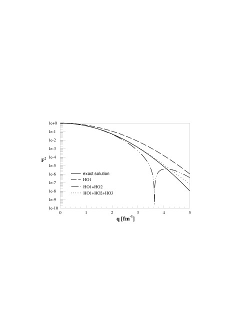
(a) ⁴He

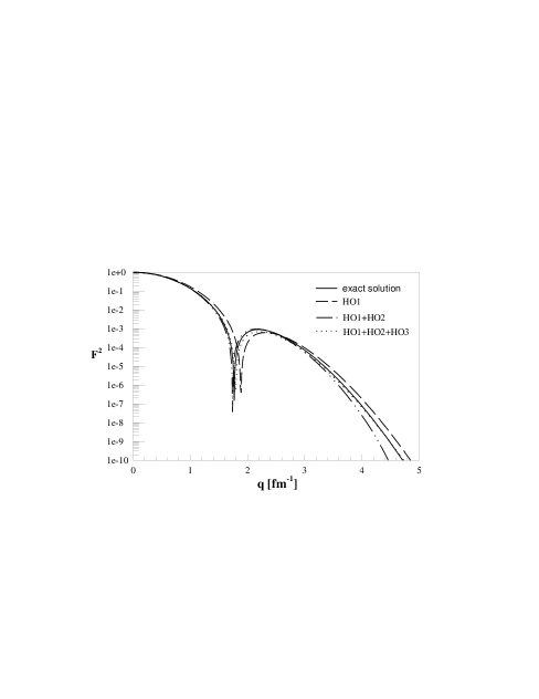
(b) ¹⁶O

FIG. 1.: Convergence of the many-body expansion (17) of the charge form factor, for the harmonic oscillator shell model case.

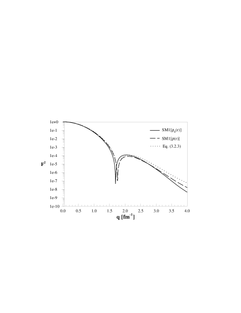
(a) Argonne $v$18

(b) Argonne $v$18 and Urbana-IX (preliminary)

FIG. 2.: ¹⁶O nucleus: $SM1[\rho_{0}(r)]$ and $SM1[\rho(r)]$ form factors compared with the internal form factor calculated according to Eq. (34).

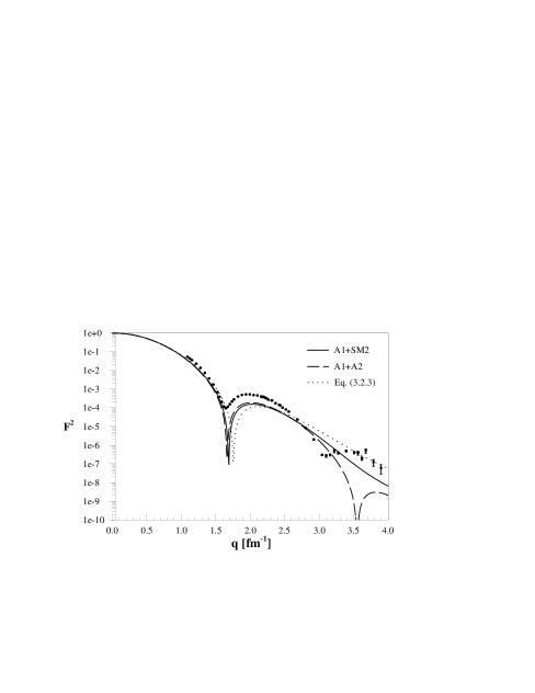
(a) Argonne $v$18

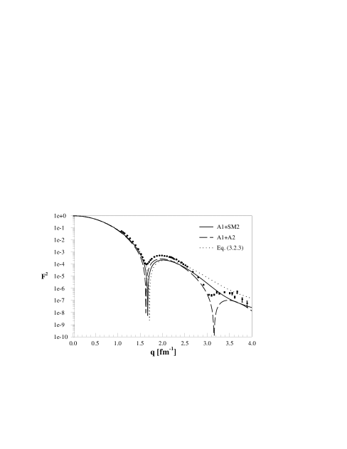
(b) Argonne $v$18 and Urbana IX (preliminary)

FIG. 3.: ¹⁶O nucleus: Two-body approximations of the translational invariant form factor compared with the internal form factor calculated according to Eq. (34).

TABLE I.: Convergence of the mean square charge radius for the case of the ⁴He and ¹⁶O nuclei.

Order of approximation	4He	16O
$\mathrm{HO1}$	1.285979	2.250000
$\mathrm{HO1}+\mathrm{HO2}$	1.484927	2.371708
$\mathrm{HO1}+\mathrm{HO2}+\mathrm{HO3}$	1.484922	2.349467
exact value	1.484924	2.349468