Ground state correlations and mean-field in 16O
Abstract
We use the coupled cluster expansion ( method) to generate the complete ground state correlations due to the interaction. Part of this procedure is the calculation of the two-body matrix inside the nucleus in which it is being used. This formalism is being applied to 16O in a configuration space of 50 . The resulting ground state wave function is used to calculate the binding energy and one- and two-body densities for the ground state of 16O.
pacs:
21.60.-n, 21.60.Gx, 21.60.Cs, 21.60.Jz, 21.10.Ft2
I Introduction
In the last thirty years electron scattering from nuclei has provided a wealth of information mapping out nuclear ground state charge densities [1], providing precise transition charge and current densities for the excitation of single particle states [2] and for collective states [3]. The measurement of ground state magnetization densities and the excitation of high multipolarity magnetic excitations, or the single particle knockout reaction to discrete states all have in some way supported the mean-field approach as the lowest order in the description of nuclear structure.
The confirmation of the mean-field approach, however, were more qualitative in nature than quantitative. The form factors e.g. for the excitation of the high spin single particle states in 208Pb [4], were described extremely well in shape by the mean-field wave functions, however, the predicted strength was too big by a factor of two. The knockout reactions again were in good agreement with the shapes predicted by the mean-field wave functions but the strength was off by again roughly a factor of two [5]. The general conclusion was that correlations are important in the calculation of observables. They do not change the shape of the wave functions but they modify the strength due to deoccupation of orbits below the Fermi surface and partial occupation of the orbits above the Fermi surface [6]. This was confirmed by (e,e′p) experiments in which particles from orbits above the Fermi level were knocked out [5]. Thus, to do justice to the accuracy of the electromagnetic probe, we can no longer be satisfied with the mean-field approach but have to take into account the correlations largely due to the hard repulsive core of the nucleon-nucleon interaction. While we put particular emphasis on the effects of correlations on the results of electron scattering experiments this is less of an issue in this paper dealing with the ground state, but will be more clearly pointed out in subsequent papers dealing with excited states of these nuclei.
There are different ways to account for correlations. One way is to introduce correlation functions in the many body wave function in real space. This has been quite successful for small nuclei [7] and has resulted in reasonable descriptions of the 16O nucleus [8]. A different approach is to add in configuration space to the uncorrelated ground state multi-particle multi-hole configurations. Both approaches can be related to each other even though it seems harder using correlation functions to satisfy the Pauli principle. In configuration space this appears to be more transparent. In our treatment we follow closely the formulation of the Bochum group [9]. However, we solve the equations entirely in configuration space. Furthermore, we truncate in different ways where the significance of terms becomes more transparent
II The uncorrelated ground state
We assume an orthonormal set of single particle wave functions exists. These wave functions are solutions to the single particle Hamiltonian given by the Schrödinger equation in the mean-field. This mean-field will be generated in an iterative procedure. The single particle wave functions are expanded in a set of orthonormal functions such as harmonic oscillator functions, Bessel functions or others. Thus each orbit is represented by a set of expansion coefficients and a single particle energy. An uncorrelated ground state can be constructed as a single Slater determinant which includes all the occupied orbits and is written as , our new vacuum state.
III Variational calculations for the correlated ground state
We use the formalism of second quantisation. As such we follow the notation of the textbook by deShalit and Feshbach [10]. In the second quantisation representation we write the Hamiltonian of a closed shell nucleus as
| (1) |
where the Einstein summation convention is understood and are fully anti-symmetric matrix elements of the potential. The orbits completely occupied in a non-correlated ground state are called “hole orbits”, those not occupied are called “particle orbits”. Creation and destruction operators in these orbits are denoted , , and , , respectively. Thus, we have
| (2) |
The correlated ground state is assumed to be of the form
| (3) |
Here is the operator that describes the correlation. It is written as
| (4) |
where
| (5) | |||||
| (6) | |||||
| (7) |
or correspondingly . The purpose of the variational calculation is to determine all the coefficients .
We will further assume that there exists at least one set of wave functions, satisfying the condition that =0. Further down we will discuss how to construct such a set. This set is the set of single particle mean-field wave functions. With that basis the lowest order of correlations are the correlations. Also, and are the same as well as and , whereas , etc.
A variation orthogonal to the correlated ground state can be constructed from any operator representing any nn-excitation as
| (8) |
We have
| (9) |
The variational principle requires that the Hamiltonian between the ground state and such a variation vanishes. Thus, we have
| (10) |
Choosing to be 11, or 22, …, AA results in a set of nonlinear coupled equations that are written out in more detail in the next section. We might say that represents the effective Hamiltonian as Eq. (10) represents the Hartree-Fock condition for the uncorrelated ground state with this effective Hamiltonian.
A The effective one-body Hamiltonian
To simplify the accounting of number of -excitations we use indices for the Hamiltonian. Explicitly we define
| (11) | |||||
| (13) | |||||
| (16) | |||||
| (17) |
We should take note that any commutes with .
We introduce the mean-field Hamiltonian as
| (18) |
where is the kinetic energy operator and is the mean-field to be specified below. We will assume that the orbits are eigenfunctions of this mean-field Hamiltonian with
| (19) |
We use Eq. (10) with , , where we write to obtain the equation establishing
| (22) | |||||
There are similar equations that determine . While these equations hold in any basis, there is one basis of particular convenience. This is the maximum overlap basis in which vanishes. Equation (22) results in the solution if the terms that do not contain vanish. The mean-field basis is determined by the condition of the vanishing of and in the mean-field basis we must have
| (24) | |||||
Using Eq. (19), we can show that the expectation value vanishes. Therefore, Eq. (24) becomes
| (25) |
Thus those terms establish the elements in the one-body Hamiltonian matrix that connect and orbits. The equations establishing the higher order correlations in the mean-field basis are
| (27) | |||||
| (31) | |||||
| (35) | |||||
At this point we will assume that the orbits are eigenfunctions to the single particle Hamiltonian . This allows us to solve these equations as
| (39) | |||||
| (42) | |||||
A similar equation allows us to isolate using Eq. (LABEL:eq:S4_eqn).
If we restrict ourselves to a situation in which only correlations are present, and become identical. Then, Eq. (39) can be written in its adjoint form as
| (43) |
This equation is essentially the Bethe-Goldstone equation for the -matrix which is normally written as [12]
| (44) |
Multiplying this equation from the left with , using and setting , results in Eq. (43) for . Thus, one of the essential parts of the coupled cluster expansion is that we calculate the ground state two-body -matrix inside the nucleus where it is to be applied. The additional terms in our coupled equations indicate the need for appropriate corrections in the -matrix for the presence of , , correlations. In most cases the -matrix is calculated in nuclear matter and then applied to finite nuclei. However, in nuclear matter the correlation function extends up to infinity and thus cannot be applied to a finite nucleus.
We estimate that in our basis there are about configurations and about configurations. While the number of configurations is quite accessible, the number of configurations is prohibitively large, and we cannot store all these numbers. Thus we have to implicitly correct for the presence of these correlations. We do this by inserting the solutions for with n3 back into the equations and thereby obtaining a perturbation expansion in . We write this equation out up to second order for the Eq. (25) establishing the mean-field
| (45) | |||
| (46) | |||
| (47) | |||
| (48) |
This equation establishes the matrix elements of the single particle Hamiltonian between particle and hole orbits. The matrix elements between hole and hole orbits or between particle and particle orbits are not defined, and any definition may be chosen. As long as is explicitly kept on the right hand side of Eqs. (39, 43) the explicit choice is merely a question of how fast the resulting series will converge. However, a reasonable choice appears to be that form that we obtain if we replace in the matrix elements obtained in Eq. (48) the hole orbit with a particle orbit in order to get the matrix elements between particle and particle orbits and we change the particle orbit into a hole orbit in order to get the matrix elements between hole and hole orbits. Reference [13] gives a detailed account of the contributions included in our mean-field as given by Eq. (48). Our choice for the other matrix elements corresponds simply in turning the hole line into a particle line or vice versa.
The mean-field orbits are the eigenvectors of this matrix, and the eigenvalues are the single particle energies. This procedure now fully defines the mean-field used here even though its definition is not unique.
To obtain values for the amplitudes of we start with Eq. (39) and replace by Eq. (42) and correspondingly . We continue with these replacements, resulting again in an expansion in for .
The calculation of the correlations breaks down into two steps: In step one the two-body correlations are computed according to Eq. (39) where the curly brackets give the various contributions to the effective matrix element. In step two the single particle energy tensor is calculated from the kinetic energy, the direct potential energy, and the correlation energy. The eigenvalues and the eigenvectors of the energy tensor give the new single particle energies and the new single particle functions. The two steps are iterated until a self-consistent solution is obtained, i.e. the energy tensor is diagonal.
As we use an infinite expansion we must truncate that expansion. We find that terms connecting to effective one-body terms give the major contributions, two-body terms are less important. Generally, we have included all terms that are written as product of three two-body operators. Of those terms written as product of four two-body operators we have included those terms where at least two operators connect to a one-body operator. This results in all the quenching terms for the products of two two-body operators. We have also included those terms that look like the terms of the products of three two-body operators with a renormalized interaction. We found that these corrections are equally significant for those terms arising from and those arising from . Left out are mostly those terms that required several angular momentum recouplings. Contributions from show up only if one considers products of more than four two-body operators. In the Ref. [13] we have listed explicitly the relations and approximations that we have used in this calculation.
IV Numerical calculations for 16O
We have solved the main Eq. (48) that determines the -amplitudes and thus essentially the ground state -matrix for 16O in a space of 50 with a harmonic oscillator length parameter b=0.8 fm, excluding those orbits with . Corrections for correlations were included in a reduced space of 30 and , while correlations due to correlations were included in the full space. We used the Argonne potential [11] to generate the matrix elements [14]. For comparison, results for the Argonne and potentials are reported. Here, the Argonne potential is the reprojection of the Argonne potential in the sense of reference [7].
The Hamiltonian is given in the center-of-mass as
| (49) |
where is the kinetic energy operator of the center-of-mass, and is the total mass. This represents the energy in the center-of-mass frame. It can be rewritten as
| (51) | |||||
The last term is treated as part of the internal potential, and the antisymmetric matrix elements of the internal potential include this center-of-mass correction term.
A Ground state expectation values for arbitrary operators
Ground state expectation values can be evaluated by introducing the operator , as described e.g. in the review by Bishop [12]. We take the ground state as
| (52) |
We have defined as the complete set of 11, 22, …, AA excitations. The normalized expectation value of any operator , , can be worked out as
| (53) |
By inserting the unity operator in the basis, we obtain
| (54) | |||
| (55) |
The expectation value on the right is by definition , the expectation value of . Thus we can define the new operator
| (56) |
With this, the expectation value for any operator can be expressed as
| (57) |
The operators can be obtained by solving Eq. (56) in an iterative fashion. Explicitly we write in the same form as Eq. (7), but use the amplitudes instead of to distinguish it from .
B Ground state binding energy
We first apply the above formalism to the ground state binding energy. The expectation value of the internal Hamiltonian can be written as
| (58) |
Because of the Hartree-Fock (HF) condition expressed in Eq. (10) the terms involving vanish and we get
| (59) |
Assuming that is at most a two-body operator and taking into account that vanishes, we write this as
| (60) |
When we evaluate the expectation values of the operators in the above equation, we have to consider that the hole orbits are not diagonal with respect to any of these operators. Also, as we have used the HF condition this expression does not give an upper limit of the ground state energy unless we are exactly at the minimum. In terms of matrix elements the energy can be written as
| (62) | |||||
The use of Eq. (62) for the energy implies that all the correlations are present and satisfy the Eqs. (10). In that case the resulting energy could be taken as an upper bound to the true energy. However, in solving these equations we have ignored some of the couplings back into . As a result Eq.(62) is no longer exact and the feature of being an upper bound to the true energy is lost. We believe that the errors due to the truncations are reasonably small. However, more experience is needed with some of the terms left out in order to reduce the uncertainties in the result. Table I shows the resulting binding energy for the Argonne , and potentials.
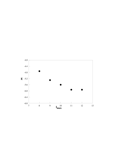
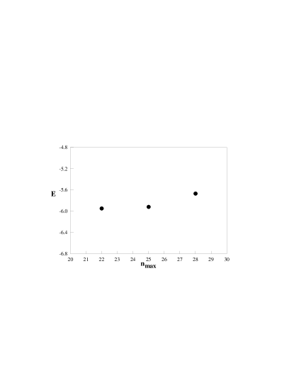
Our Hilbert space is controlled by two cut-off parameters and , which are related to the size of the Hilbert space as . We have studied the dependence of the binding energy on these two parameters. Figure 1 displays the dependence and shows reasonable convergence for . This dependence was mapped out with =25. We have also checked the sensitivity of the binding energy with respect to with a fixed . In this case, we find that for our choice of a 30 space, the binding energy is independent of for an value between 22 and 25. As we go to larger values however, we start seeing the effect of having a smaller space and the approximation starts breaking down. The dependence of the binding energy on the cut-off is depicted in Fig. 2 for =11.
C Ground state one-body density
Next, we apply this procedure to the ground state one-body density. The expressions necessarily look more complex as we cannot apply the HF condition to simplify the expressions.
By definition, the ground state one-body density is introduced as
| (63) |
Since we are dealing with a spherically symmetric system, we shall integrate out the angular degrees of freedom of the system. Then, we write the density operator in the second quantisation representation as
| (64) |
Here we use to denote the radial part of the expectation value . Thus, we can write the ground state density as
| (65) |
where
| (66) |
is the density matrix. The density matrix is a real symmetric matrix with positive definite eigenvalues. We can make a basis transformation such that the density matrix becomes diagonal. This basis represents the “natural” orbits. In this basis the density becomes
| (67) |
Here represents the occupation probability of these natural orbits. This is the only basis in which occupation probabilities have a meaning.
To calculate the one-body density matrix we use Eq. (66) with Eq. (57)
| (68) | |||
| (69) | |||
| (70) | |||
| (71) |
In evaluating terms of equal order we have to consider to be of order , to be of order , to be of order , etc. To account for and we have to use the expansions of Eq. (39). As vanishes, is of the same order as . Otherwise is of the same order as .
The one-body density calculated this way is not the density in the center-of-mass frame of the nucleus as the wave function represents a nucleus that has a residual center-of-mass motion. The form factor measured in experiments is the form factor in the center-of-mass frame which we can write as
| (72) |
i.e. the form factor calculated from the one-body density factorizes into the form factor in the center-of-mass frame and the form factor of the center-of-mass motion .
It has been shown that for a pure uncorrelated harmonic oscillator wave function this form factor can be written as where is the harmonic oscillator length parameter. There are two reasons why this does not apply here. First, we have self-consistent mean-field wave functions and not harmonic oscillator wave functions and second, we have not a single Slater determinant but a sum over many due to the correlations. For these reasons we chose to evaluate the form factor directly using Eq. (72). By writing , the Eq. (72) is expanded into n-body terms. This expansion was checked for the case of a single Slater determinant of harmonic oscillator functions against the exact result. It was found that this expansion is quite satisfactory if all terms up to three-body terms are kept [15].
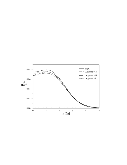
Fig. 3 shows the calculated charge density after folding the proton point density with the charge density of the proton and folding the neutron point density with the charge density of the neutron. As this expansion is accurate up to terms of order , it encompasses the result of the rms-radius. At the present time no corrections due to the meson-exchange charge density are taken into account. The resulting charge radii are shown in Table I for the Argonne , and potentials, respectively, and are reasonably close to the experimental one.
In the calculation of the natural orbits we also generate the occupation probabilities for the orbits above the Fermi level. For the Argonne , and potentials the occupation probabilities of the 1 and the 2 proton orbits are summarized in Table I and appear to be consistent with the experiment [5], which establishes a lower limit for these values.
D Ground state two-body density
A direct presentation of the short range correlation can be seen in the ground state two-body density. We start with the ground state two-body density definition
| (73) |
In the second quantization representation the two-body density operator can be written as
| (74) |
Using the completeness relationship of the spherical harmonics we can evaluate the matrix element
| (76) | |||
| (77) | |||
| (78) |
In order to be consistent with the phase convention of the two-body potential matrix elements, we couple the two-body density matrix elements using the ph angular momentum coupling conventions [14]. Then, the angular momentum coupled density is
| (80) | |||
| (81) |
Here we have introduced the one-body multipole density which is
| (82) | |||||
| (84) | |||||
if is even, and zero otherwise.
For a spherically symmetric (spin=0) nucleus it is more relevant to calculate as due to the spherical symmetry the two-body density is dependent on the direction of relative to alone. Thus, we can perform an average over the directions of . This translates into carrying out the sum over the component of the angular momentum . We obtain the result
| (85) |
We now discuss the most dominant contributions. We again apply Eq. (57) to evaluate the two-body density matrix, . With this, we get the ground state two-body density as
| (86) | |||
| (87) | |||
| (88) | |||
| (89) |
(a)Contributions from bare ground state:
| (90) | |||
| (91) |
This term has the structure . Here is the bare one-body density. We can include all higher order one-body density terms by adding
| (92) |
where is the difference between the full one-body density minus the bare one-body density. In turn, in higher order terms we have to exclude those terms where in the operator connects with or connects with . However, we still have to consider the exchange terms where connects with and connects with .
The exchange term is due to the Pauli correlations and results in
| (93) | |||
| (94) |
(b) Contributions linear in the -amplitudes. For the following terms we assume a summation over all orbits appearing twice in the expression. The leading term that arises from the correlations is
| (96) | |||||
In our application we have included all terms up to second order. Aside from the terms listed here, the next most important correction arises from the second order term depending on and .
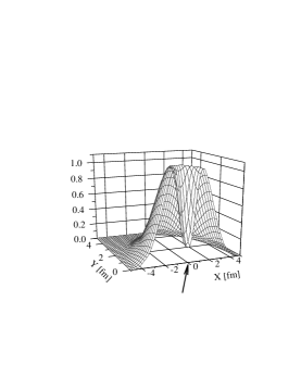
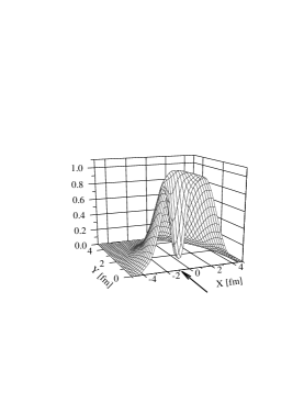
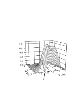
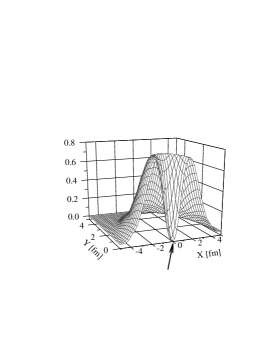
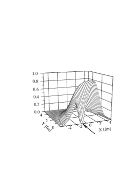
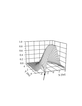
The two-body density represents the probability of finding one nucleon at and one nucleon at . We can divide this by the probability of finding the first nucleon at . The remaining density represents the probability of finding a second nucleon at if the first nucleon is at . If both nucleons are protons, this density is normalised to a total integral of (Z-1). Figs. 4 to 9 show these densities as a function of for various positions of . We have made no attempt to correct these for the residual center-of-mass motion of the nucleus. The densities show the effects of the short range repulsion: they exhibit a deep hole where the first nucleon is located. The two-body densities also show that for large distances the long-range aspect of the ground state nuclear correlations, usually thought to be related with the surface deformation modes, has a significant contribution: when the first nucleon is located closer to the nuclear surface, we observe an enhancement of the density at the symmetrically-opposite position. The picture of a two-body density obtained as the revolution of the spherically symmetric one-body density, with a Gaussian-like distribution centered at the location of the first nucleon scooped out of it, is definitely insufficient.
V Conclusions
We use the coupled cluster expansion ( method) to solve the many-body Schrödinger equation in configuration space. While the coupled cluster expansion is exact if carried out to all orders, the present results are obtained with truncations. As we have retained only terms up to second order in the contributions from have no effect on . In turn, the effects of any higher correlations are only of the order as the higher order terms left out anyway. Thus, in essence we have replaced the truncations in by the more relevant truncation in .
We have shown that it is possible to choose large enough configuration spaces for the complete and self-consistent calculation of the ground state correlations inside a finite nucleus. This calculation makes no artificial separation between “short range” and “long range” correlations. In fact, the two-body density shows that the correlation function in the surface region of the nucleus has strong contributions from the surface deformation modes. It is largely these modes that cause the strong deoccupation of orbits close to the Fermi surface. The occupation of the 2 and the 1 proton orbits calculated is consistent with the values suggested by the experiments.
Our efforts are currently directed in two directions. First, we intend to apply the procedure described in this paper to the particular case of a more realistic interaction, namely the Argonne potential [11] together with a phenomenological three-nucleon interaction [16]. This should not only result in a better description of the 16O observables, but a breakdown of the contributions to the binding from the two- and the three-body interactions could be inferred also. Secondly, we shall use the equation of motion technique to calculate excited states of the 16O nucleus, and the ground state and excited states of the neighboring nuclei (e.g. 15N). We hope to be able to present our findings in the near future.
acknowledgements
This work was supported by the U.S. Department of Energy (DE-FG02-87ER-40371). Original calculations were carried out on a HP-9000/735 workstation at the Research Computing Center, and a dual-processor 200 MHz Pentium Pro PC at the Nuclear Physics Group of the University of New Hampshire. The authors gratefully acknowledge the help of Mike Strayer and David Dean in letting us use their computing resources for the mapping of the binding energy with respect to the size of the configuration space. These calculations were carried out on a 180 MHz R10000 Silicon Graphics Workstation at the Computational and Theoretical Physics Section ORNL. The authors gratefully acknowledge John Dawson for his permanent support in every step of this project. The authors also acknowledge helpful conversations with Vijay Pandharipande and Robert Wiringa, who also supplied the Fortran subroutines to calculate the radial shape of the interaction.
REFERENCES
- [1] J. M. Cavedon, Thesis de Doctoral d’Etat, Paris (1980)
- [2] O. Schwentker, J. Dawson, J. Robb, J. Heisenberg, J. Lichtenstadt, C. N. Papanicolas, J. Wise, J. S. McCarthy, L. T. van der Bijl, and H. P. Blok, Phys. Rev. Lett. 50, 15 (1983).
- [3] D. Goutte, J. B. Bellicard, J. M. Cavedon, B. Frois, M. Huet, P. LeConte, Phan Xuan Ho, S. Platchkov, J. Heisenberg, J. Lichtenstadt, C. N. Papanicolas, and I. Sick, Phys. Rev. Lett. 45, 1618 (1980).
- [4] J. Lichtenstadt, J. Heisenberg, C. N. Papanicolas, C. P. Sargent, A. N. Courtemanche, and J. S. McCarthy, Phys. Rev. C 20, 497 (1979).
- [5] M. Leuschner, J. R. Calarco, F. W. Hersman, H. P. Blok, G. J. Kramer, L. Lapikás, G. van der Steenhoven, P. K. A. de Witt Huberts, and J. Friedrich, Phys. Rev. C 49, 955 (1994).
- [6] V. R. Pandharipande, C. N. Papanicolas, and J. Wambach, Phys. Rev. Lett. 53, 1133 (1984).
- [7] B. S. Pudliner, V. R. Pandharipande, J. Carlson, S. C. Pieper, and R. B. Wiringa, Phys. Rev. C 56, 1720 (1997); B. S. Pudliner, V. R. Pandharipande, J. Carlson, and R. B. Wiringa, Phys. Rev. Lett. 74, 4396 (1995).
- [8] S. C. Pieper, R. B. Wiringa, and V. R. Pandharipande, Phys. Rev. C 46, 1747 (1992).
- [9] H. Kümmel, K. H. Lührmann, and J. G. Zabolitzky, Phys. Reports 36, 1 (1978).
- [10] A. deShalit and H. Feshbach, Theoretical Nuclear Physics, Vol. I, John Wiley & Sons, Inc (1974)
- [11] R. B. Wiringa, V. G. Stoks, and R. Schiavilla, Phys. Rev. C 51, 38 (1995).
- [12] R. F. Bishop, Theor. Chim. Acta 80, 95 (1991).
- [13] J. H. Heisenberg and B. Mihaila, nucl-th/9802031 (1998).
- [14] B. Mihaila and J. H. Heisenberg, nucl-th/9802012 (1998).
- [15] B. Mihaila and J. H. Heisenberg, nucl-th/9802032 (1998).
- [16] J. Carlson, V.R. Pandharipande, and R.B. Wiringa, Nucl. Phys. A 401, 59 (1983).
| Potential | E | rms | 1 | 2 |
|---|---|---|---|---|
| [MeV/nucleon] | [fm] | [%] | [%] | |
| 8 | - 7.0 | 2.81 | 3.68 | 4.09 |
| 14 | - 6.1 | 2.86 | 3.33 | 3.99 |
| 18 | - 5.9 | 2.81 | 2.58 | 2.75 |
| expt. | - 8.0 | 2.73 | 2.17 | 1.78 |
| 0.025 | 0.12 | 0.36 |